Nonlinear temperature effects on multifractal complexity of metabolic rate of mice
- Published
- Accepted
- Subject Areas
- Computational Biology, Ecology, Mathematical Biology, Statistics
- Keywords
- Physiological complexity, metabolic rate fluctuations, Endothermy, Mus musculus, long-range correlations, multifractality, Metabolic rate
- Copyright
- © 2016 Labra et al.
- Licence
- This is an open access article distributed under the terms of the Creative Commons Attribution License, which permits unrestricted use, distribution, reproduction and adaptation in any medium and for any purpose provided that it is properly attributed. For attribution, the original author(s), title, publication source (PeerJ Preprints) and either DOI or URL of the article must be cited.
- Cite this article
- 2016. Nonlinear temperature effects on multifractal complexity of metabolic rate of mice. PeerJ Preprints 4:e2404v1 https://doi.org/10.7287/peerj.preprints.2404v1
Abstract
Complex physiological dynamics have been argued to be a signature of healthy physiological function. Here we test whether the complexity of metabolic rate fluctuations in small endotherms decreases with lower environmental temperatures. To do so we examine the multifractal temporal scaling properties of the rate of change in oxygen consumption r(VO2), in the laboratory mouse Mus musculus, assessing their long range correlation properties across 7 different environmental temperatures, ranging from 0°C to 30°C. To do so, we applied multifractal detrended fluctuation analysis (MF-DFA), finding that r(VO2) fluctuations show two scaling regimes. For small time scales below the crossover time (approximately 102 seconds), either monofractal or weak multifractal dynamics are observed depending on whether Ta<15°C or Ta > 15°C respectively. For larger time scales, r(VO2) fluctuations are characterized by an asymptotic scaling exponent that indicates multifractal anti-persistent or uncorrelated dynamics. For both scaling regimes, a generalization of the multiplicative cascade model provides very good fits for the Renyi exponents τ(q), showing that the infinite number of exponents h(q) can be described by only two independent parameters, a and b. We also show that the long-range correlation structure of r(VO2) time series differs from randomly shuffled series, and may not be explained as an artifact of stochastic sampling of a linear frequency spectrum. These results show that metabolic rate dynamics in a well studied micro-endotherm are consistent with a highly non-linear feedback control system.
Author Comment
This is a submission to PeerJ for review.
Supplemental Information
Nonlinear temperature effects on multifractal complexity of metabolic rate
The data shows individual time series for 18 mice assigned at random to seven different temperature treatments. Given that experimental records differed in total length, data in the matrix have been padded with "nan" codes. For every time series, we provide the original experimental code, individual body mass measured after metabolic rate recording, and environmental temperature at which the metabolic rate signal was registered.
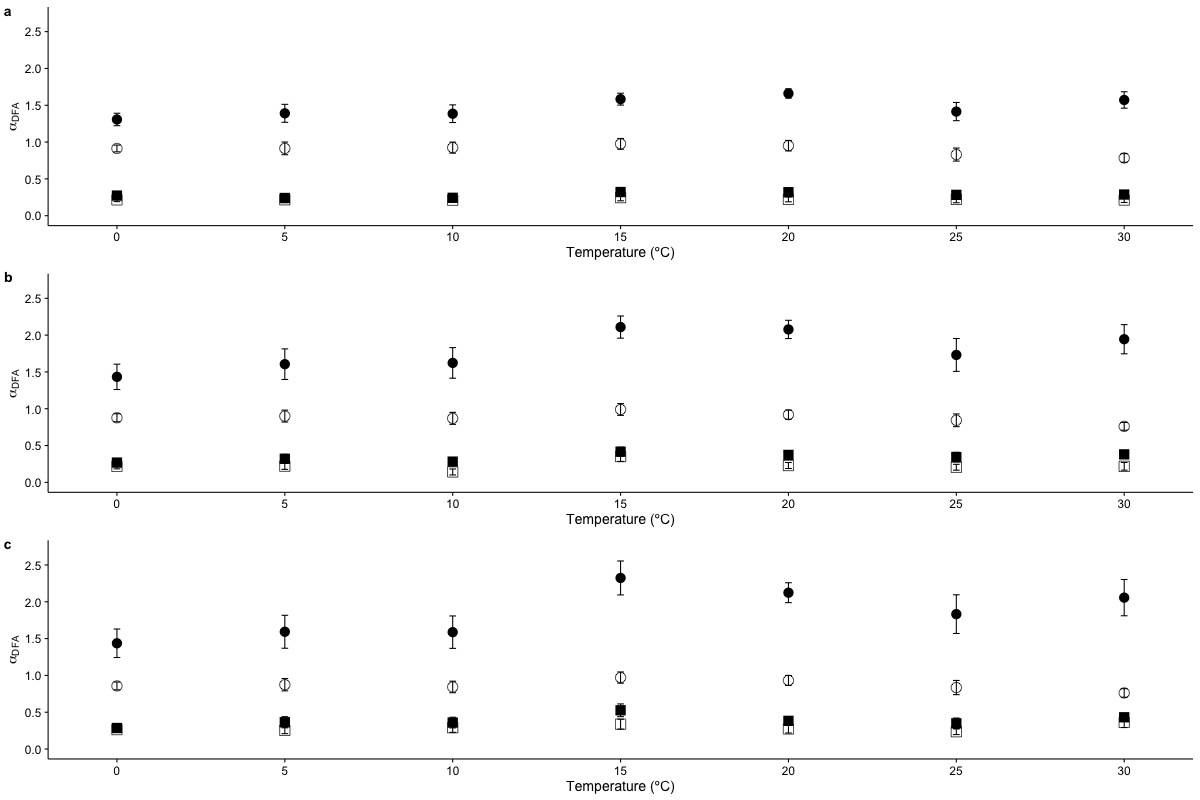
Supplementary Figure 1: Temperature effects on long range scaling exponent αDFA in metabolic rate fluctuations
The figure shows the average DFA scaling exponent αDFA calculated as a function of experimental temperature for (a) Linear DFA de-trending, (b) quadratic polynomial de-trending and (c) cubic de-trending. Average scaling exponents corresponding to exponent for raw r(VO2) data within the 10 < s < 100 scaling regime are shown with filled circles, while filled squares show the scaling exponents for the raw r(VO2) data within the 100 < s < 1024 scaling regimes are shown with. Open circles and squares show the scaling exponents for these two respective scaling regimes when data are shuffled.
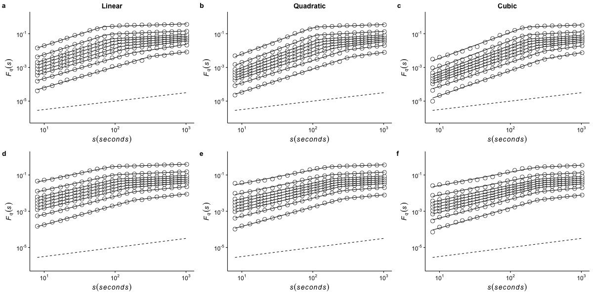
Supplementary Figure 2:Effects of de-trending polynomial order on the generalized fluctuation function of r(VO2) measured at 0ºC
The figure shows the average generalized fluctuation function Fq(s) vs. time scale s in log-log plots for r(VO2) fluctuations using different de-trending orders. Figures in the top row show average results calculated for the raw time series measured at Ta= 0ºC when data are detrended using (a) a linear function, (b) a quadratic polynomial and (c) a cubic polynomial. The bottom row shows the results for the shuffled time series when the data are detrended using (d) a linear function, (e) a quadratic polynomial and (f) a cubic polynomial. Open circles show the observed Fq(s) values for different values of q, with q = 8, 4, 2,1,0, -1,-2, -4, and -8 (from the top to the bottom). All curves are shifted vertically for clarity. The straight lines are best piecewise linear regression fits to the Fq(s) functions. Dashed straight lines with slope h=0.5 are shown below the data in each figure to allow qualitative comparison with the uncorrelated case.
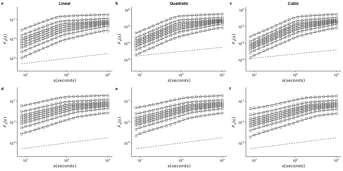
Supplementary Figure 3: Effects of de-trending polynomial order on the generalized fluctuation function of r(VO2) measured at 5ºC
The figure shows the average generalized fluctuation function Fq(s) vs. time scale s in log-log plots for r(VO2) fluctuations using different de-trending orders. Figures in the top row show average results calculated for the raw time series measured at Ta= 5ºC when data are detrended using (a) a linear function, (b) a quadratic polynomial and (c) a cubic polynomial. The bottom row shows the results for the shuffled time series when the data are detrended using (d) a linear function, (e) a quadratic polynomial and (f) a cubic polynomial. Open circles show the observed Fq(s) values for different values of q, with q = 8, 4, 2,1,0, -1,-2, -4, and -8 (from the top to the bottom). All curves are shifted vertically for clarity. The straight lines are best piecewise linear regression fits to the Fq(s) functions. Dashed straight lines with slope h=0.5 are shown below the data in each figure to allow qualitative comparison with the uncorrelated case.
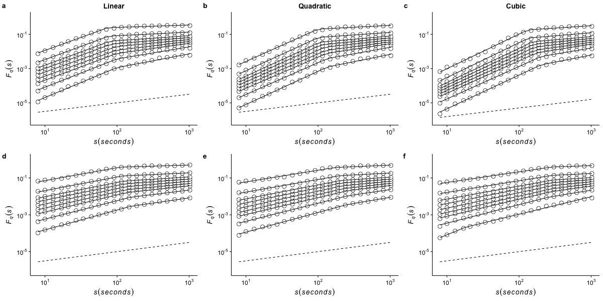
Supplementary Figure 4: Effects of de-trending polynomial order on the generalized fluctuation function of r(VO2) measured at 10ºC
The figure shows the average generalized fluctuation function Fq(s) vs. time scale s in log-log plots for r(VO2) fluctuations using different de-trending orders. Figures in the top row show average results calculated for the raw time series measured at Ta= 10ºC when data are detrended using (a) a linear function, (b) a quadratic polynomial and (c) a cubic polynomial. The bottom row shows the results for the shuffled time series when the data are detrended using (d) a linear function, (e) a quadratic polynomial and (f) a cubic polynomial. Open circles show the observed Fq(s) values for different values of q, with q = 8, 4, 2,1,0, -1,-2, -4, and -8 (from the top to the bottom). All curves are shifted vertically for clarity. The straight lines are best piecewise linear regression fits to the Fq(s) functions. Dashed straight lines with slope h=0.5 are shown below the data in each figure to allow qualitative comparison with the uncorrelated case.
Supplementary Figure 5:Effects of de-trending polynomial order on the generalized fluctuation function of r(VO2) measured at 15ºC
The figure shows the average generalized fluctuation function Fq(s) vs. time scale s in log-log plots for r(VO2) fluctuations using different de-trending orders. Figures in the top row show average results calculated for the raw time series measured at Ta= 15ºC when data are detrended using (a) a linear function, (b) a quadratic polynomial and (c) a cubic polynomial. The bottom row shows the results for the shuffled time series when the data are detrended using (d) a linear function, (e) a quadratic polynomial and (f) a cubic polynomial. Open circles show the observed Fq(s) values for different values of q, with q = 8, 4, 2,1,0, -1,-2, -4, and -8 (from the top to the bottom). All curves are shifted vertically for clarity. The straight lines are best piecewise linear regression fits to the Fq(s) functions. Dashed straight lines with slope h=0.5 are shown below the data in each figure to allow qualitative comparison with the uncorrelated case.
Supplementary Figure 6:Effects of de-trending polynomial order on the generalized fluctuation function of r(VO2) measured at 20ºC
The figure shows the average generalized fluctuation function Fq(s) vs. time scale s in log-log plots for r(VO2) fluctuations using different de-trending orders. Figures in the top row show average results calculated for the raw time series measured at Ta= 20ºC when data are detrended using (a) a linear function, (b) a quadratic polynomial and (c) a cubic polynomial. The bottom row shows the results for the shuffled time series when the data are detrended using (d) a linear function, (e) a quadratic polynomial and (f) a cubic polynomial. Open circles show the observed Fq(s) values for different values of q, with q = 8, 4, 2,1,0, -1,-2, -4, and -8 (from the top to the bottom). All curves are shifted vertically for clarity. The straight lines are best piecewise linear regression fits to the Fq(s) functions. Dashed straight lines with slope h=0.5 are shown below the data in each figure to allow qualitative comparison with the uncorrelated case.
Supplementary Figure 7: Effects of de-trending polynomial order on the generalized fluctuation function of r(VO2) measured at 25ºC
The figure shows the average generalized fluctuation function Fq(s) vs. time scale s in log-log plots for r(VO2) fluctuations using different de-trending orders. Figures in the top row show average results calculated for the raw time series measured at Ta= 25ºC when data are detrended using (a) a linear function, (b) a quadratic polynomial and (c) a cubic polynomial. The bottom row shows the results for the shuffled time series when the data are detrended using (d) a linear function, (e) a quadratic polynomial and (f) a cubic polynomial. Open circles show the observed Fq(s) values for different values of q, with q = 8, 4, 2,1,0, -1,-2, -4, and -8 (from the top to the bottom). All curves are shifted vertically for clarity. The straight lines are best piecewise linear regression fits to the Fq(s) functions. Dashed straight lines with slope h=0.5 are shown below the data in each figure to allow qualitative comparison with the uncorrelated case.
Supplementary Figure 8: Effects of detrending polynomial order on the generalized fluctuation function of r(VO2) measured at 30ºC
The figure shows the average generalized fluctuation function Fq(s) vs. time scale s in log-log plots for r(VO2) fluctuations using different detrending orders. Figures in the top row show average results calculated for the raw time series measured at Ta= 30ºC when data are detrended using (a) a linear function, (b) a quadratic polynomial and (c) a cubic polynomial. The bottom row shows the results for the shuffled time series when the data are detrended using (d) a linear function, (e) a quadratic polynomial and (f) a cubic polynomial. Open circles show the observed Fq(s) values for different values of q, with q = 8, 4, 2,1,0, -1,-2, -4, and -8 (from the top to the bottom). All curves are shifted vertically for clarity. The straight lines are best piecewise linear regression fits to the Fq(s) functions. Dashed straight lines with slope h=0.5 are shown below the data in each figure to allow qualitative comparison with the uncorrelated case.
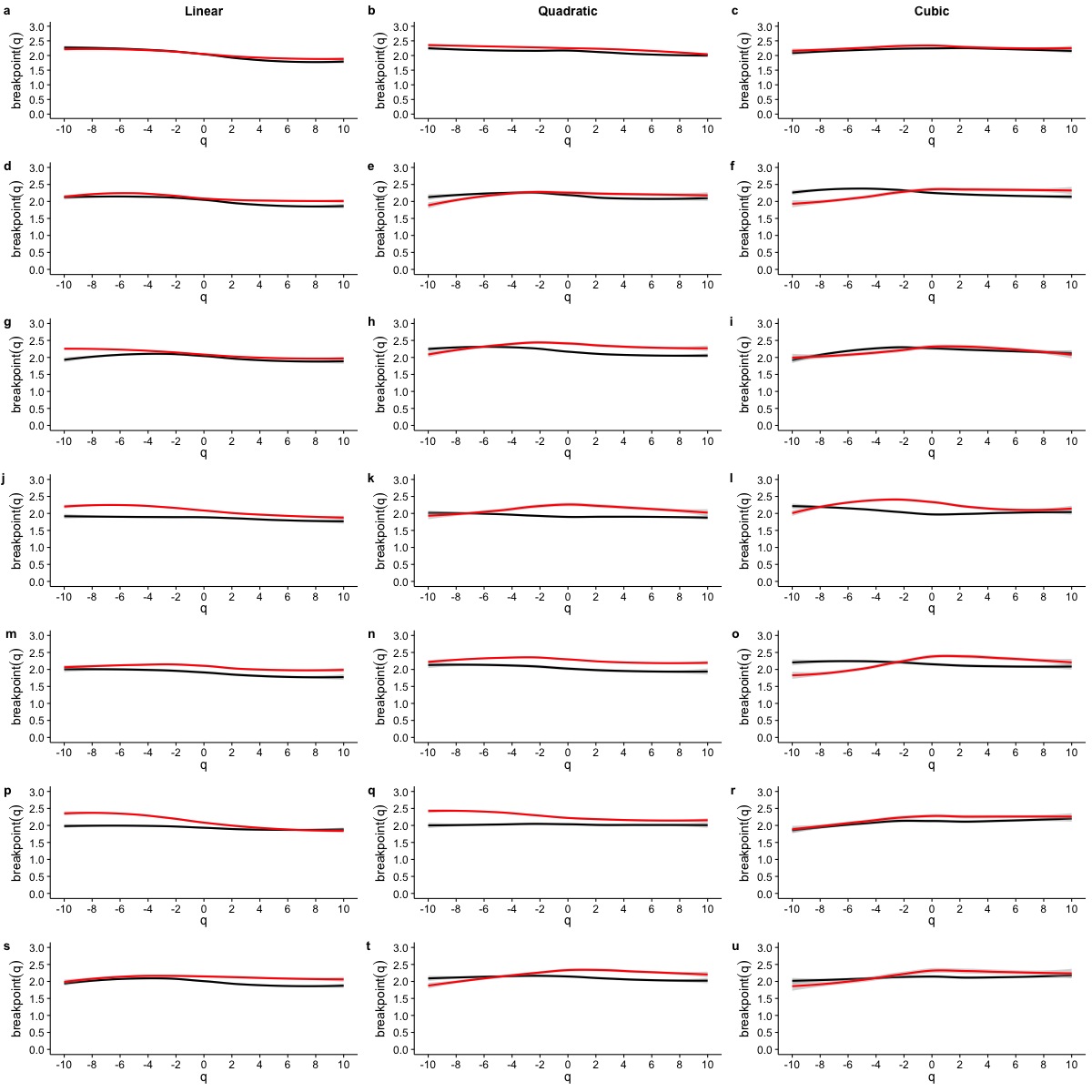
Supplementary Figure 9: Effects of temperature and detrending polynomial order on the breakpoint δ of the generalized fluctuation function Fq(s)
Top to bottom rows show the results for Ta=0ºC to Ta=30ºC respectively. Left hand, central and right hand columns show the results for linear, quadratic and cubic de-trending polynomials respectively. In all figures, black lines show the smoothed conditional mean estimate of the breakpoint, while red lines show the smoothed conditional mean estimates for shuffled data.
Supplementary Figure 10: Temperature effects on the goodness of fit of Renyi exponent spectra (τ(q)) to MMCM
The figure shows the average coeficient of determination (R2) for the fit of Renyi exponent spectra (τ(q)) to MMCM under different temperature treatments. Average R2 value in raw r(VO2) data is shown for (a) Linear de-trending, (b) quadratic polynomial de-trending and (c) cubic de-trending. Average R2 value in AAFT shuffled r(VO2) data is shown for (d) Linear de-trending, (e) quadratic polynomial de-trending and (f) cubic de-trending. Average R2 values for r(VO2) data within the 10 < s < 100 scaling regime are shown with filled circles, while open circles show average R2 values for r(VO2) data within the 100 < s < 1024 scaling regime.
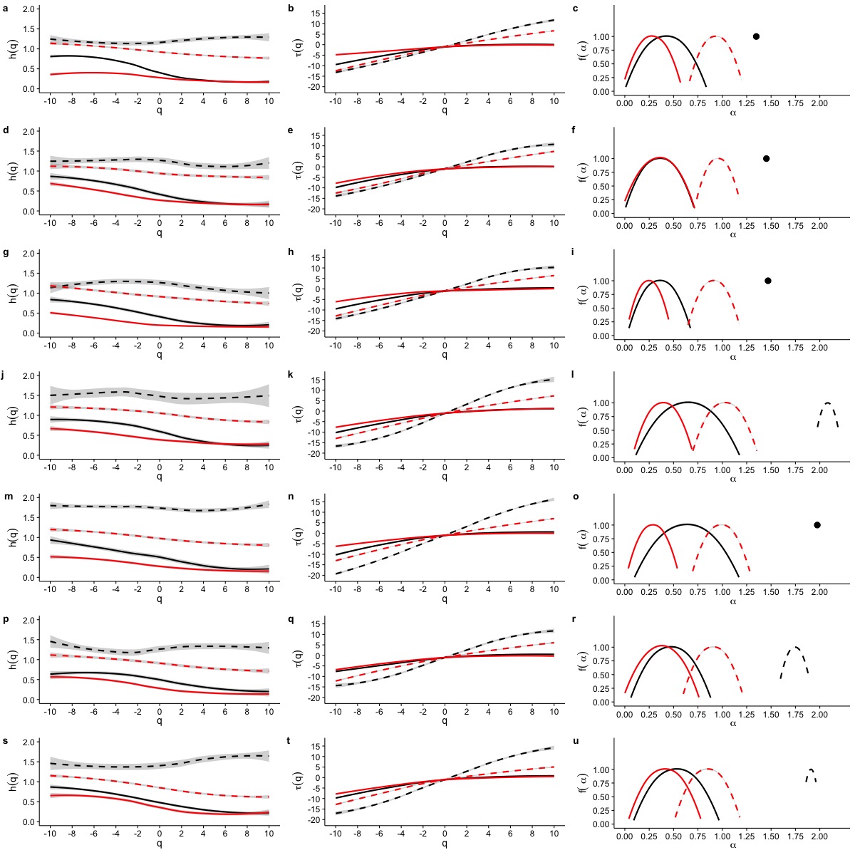
Supplementary Figure 11: MF-DFA. Effect of quadratic de-trending on Multifractal Detrended Fluctuation Analysis of Mus musculus r(VO2) time series across different temperature treatments
The figure shows the effects of quadratic de-trending on the multifractal scaling analysis for all mice studied. Left, central and right hand column show the results for the generalized Hurst exponent spectra (h(q)), Renyi exponent spectra (τ(q)) and singularity spectra (f(α)). Each figure shows the smoothed conditional mean of the different spectra in dashed and continuous black lines, representing data for the first and second scaling regimes respectively. For shuffled data, dashed and continuous red lines show the smoothed conditional mean of the different spectra for the first and second scaling regimes respectively. For figures (c), (f), (i) and (o), the singularity spectra of the first regime corresponds to a single point, shown by a filled circle. The singularity spectra reveal that for temperatures in the range 0ºC < Ta < 10ºC the time scales in the 8 < s < 100 range present a monofractal scaling, while all remaining temperatures show a weak multifractal scaling. All data for the second scaling regime show strong multifractality.
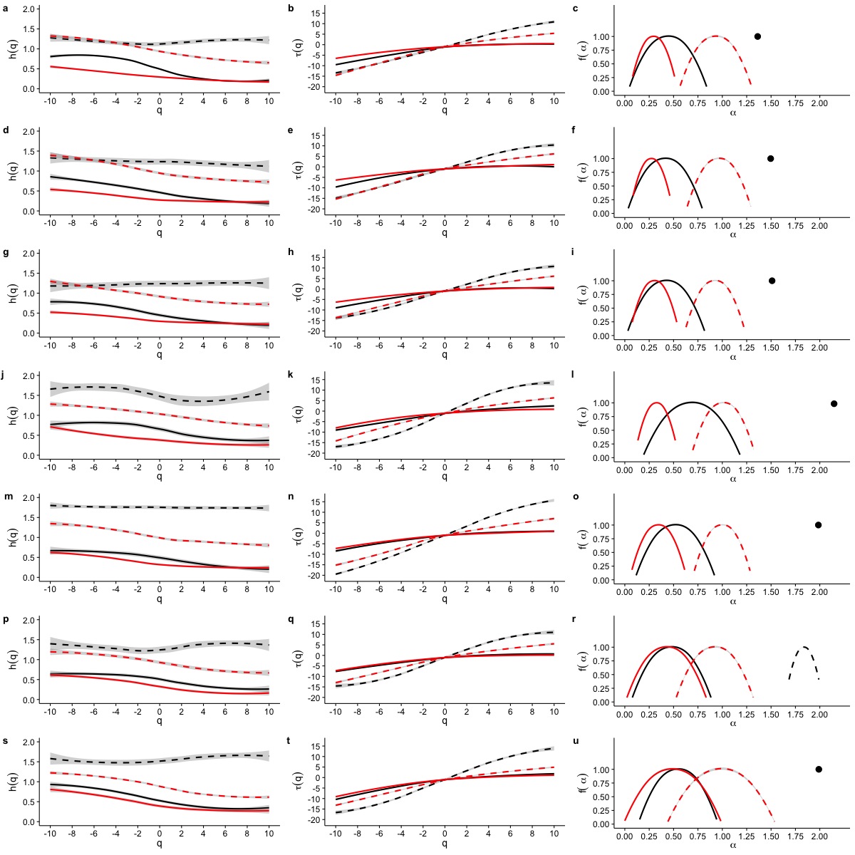
Supplementary Figure 12: MF-DFA. Effect of cubic de-trending on Multifractal Detrended Fluctuation Analysis of Mus musculus r(VO2) time series across different temperature treatments
The figure shows the effects of cubic de-trending on the multifractal scaling analysis for all mice studied. Left, central and right hand column show the results for the generalized Hurst exponent spectra (h(q)), Renyi exponent spectra (τ(q)) and singularity spectra (f(α)). Each figure shows the smoothed conditional mean of the different spectra in dashed and continuous black lines, representing data for the first and second scaling regimes respectively. For shuffled data, dashed and continuous red lines show the smoothed conditional mean of the different spectra for the first and second scaling regimes respectively. For figures (c), (f), (i), (l), (o) and (u) the singularity spectra of the first regime corresponds to a single point, shown by a filled circle. The singularity spectra reveal that for all temperatures the time scales in the 8 < s < 100 range present either a monofractal scaling or a weak multifractal scaling. On the other hand, all data for the second scaling regime show strong multifractality.