Generation of high order geometry representations in octree meshes
- Published
- Accepted
- Subject Areas
- Computer Aided Design, Scientific Computing and Simulation
- Keywords
- polynomial approximation, discontinuous Galerkin, mesh generation, high-order
- Copyright
- © 2015 Klimach et al.
- Licence
- This is an open access article distributed under the terms of the Creative Commons Attribution License, which permits unrestricted use, distribution, reproduction and adaptation in any medium and for any purpose provided that it is properly attributed. For attribution, the original author(s), title, publication source (PeerJ PrePrints) and either DOI or URL of the article must be cited.
- Cite this article
- 2015. Generation of high order geometry representations in octree meshes. PeerJ PrePrints 3:e1316v2 https://doi.org/10.7287/peerj.preprints.1316v2
Abstract
We propose a robust method to convert triangulated surface data into polynomial volume data. Such polynomial representations are required for high-order partial differential solvers, as low-order surface representations would diminish the accuracy of their solution. Our proposed method deploys a first order spatial bisection algorithm to find robustly an approximation of given geometries. The resulting voxelization is then used to generate Legendre polynomials of arbitrary degree. By embedding the locally defined polynomials in cubical elements of a coarser mesh, this method can reliably approximate even complex structures, like porous media. It thereby is possible to provide appropriate material definitions for high order discontinuous Galerkin schemes. We describe the method to construct the polynomial and how it fits into the overall mesh generation. Our discussion includes numerical properties of the method and we show some results from applying it to various geometries. We have implemented the described method in our mesh generator Seeder, which is publically available under a permissive open-source license.
Author Comment
Updated version of the manuscript after reviewer comments. This version has an improved description of the algorithm and flow-chart to illustrate it more clearly. A new section was added to show the application of the geometry generation in an electrodynamic simulation.
Supplemental Information
Illustration of the voxelization process for a sphere
Illustration of the voxelization of a sphere within coarse mesh elements. The sphere is indicated by the yellow surface while the thick black lines outline the elements of the actual mesh. The voxelization within elements follows the Octree refinement towards the sphere and is indicated by the thinner white lines. Inside the sphere, voxels have been colorized by the flood-fill mechanism with a seed in the center. Flooded elements are shown in red; other elements are blue.
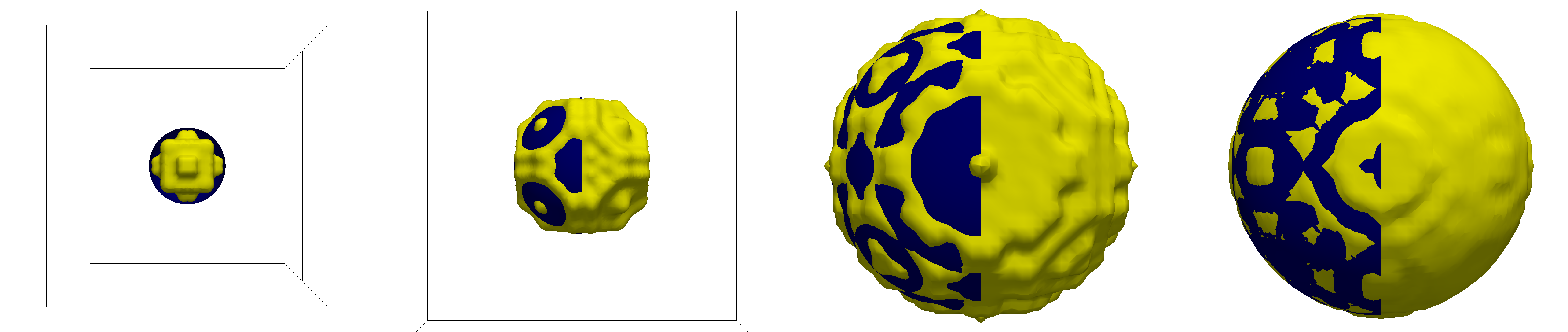
Illustration of sphere approximations with various accuracy
Illustration of sphere approximations, with increasing accuracy. The sphere is blue, and the isosurface of the color value at 0.5 is yellow. On the left, the sphere is shown in the embedding domain with the 8 elements. Voxelization and integration points increase from left to right.
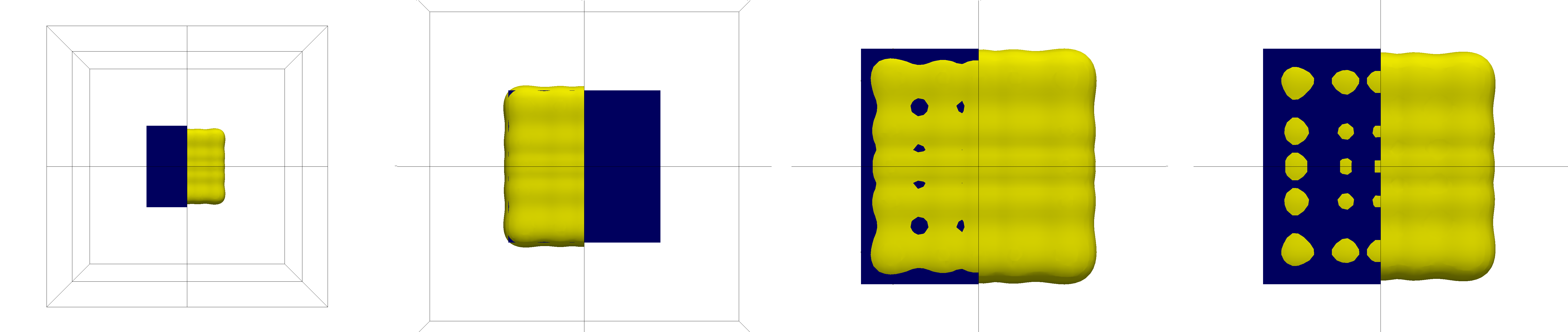
Illustration of varying number of integration points for a cube
Representation of the cube in 8 elements with polynomials of degree 15. From left to right an increasing number of integration points is used. The leftmost image shows the cube with the 8 elements of the mesh. The reference geometry is drawn in blue, and the isosurface of the color value 0.5 in yellow. We cut the reference in the middle to enable a better view for the comparison, except for the second image, where it is the other way around, and the isosurface is cut.
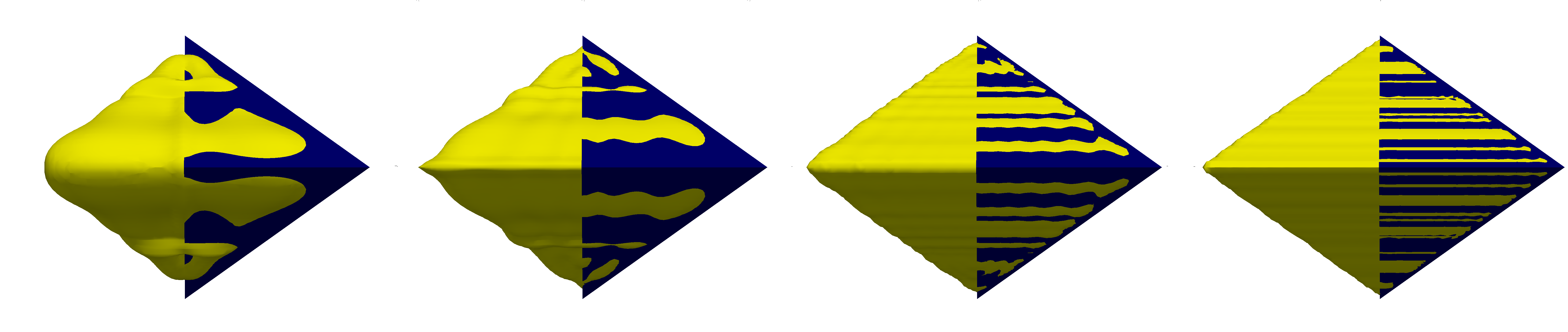
Illustration of varying polynomial degrees in the approximation of a tetrahedron
Approximation of the tetrahedron with an increasing polynomial degree from left to right. Starting on the left with a polynomial degree of 7 and increasing over 15 and 31 to 63 in the rightmost image. Shown is the isosurface of the polynomial at a value of 0.5 in yellow and for comparison the reference geometry cut in half with a blue coloring.
Example for the application to a complex geometry like a porous medium
Isosurface of a porous medium (yellow) in comparison to the original STL data (blue). The geometry is well recovered; only edges are smoothed out a little.
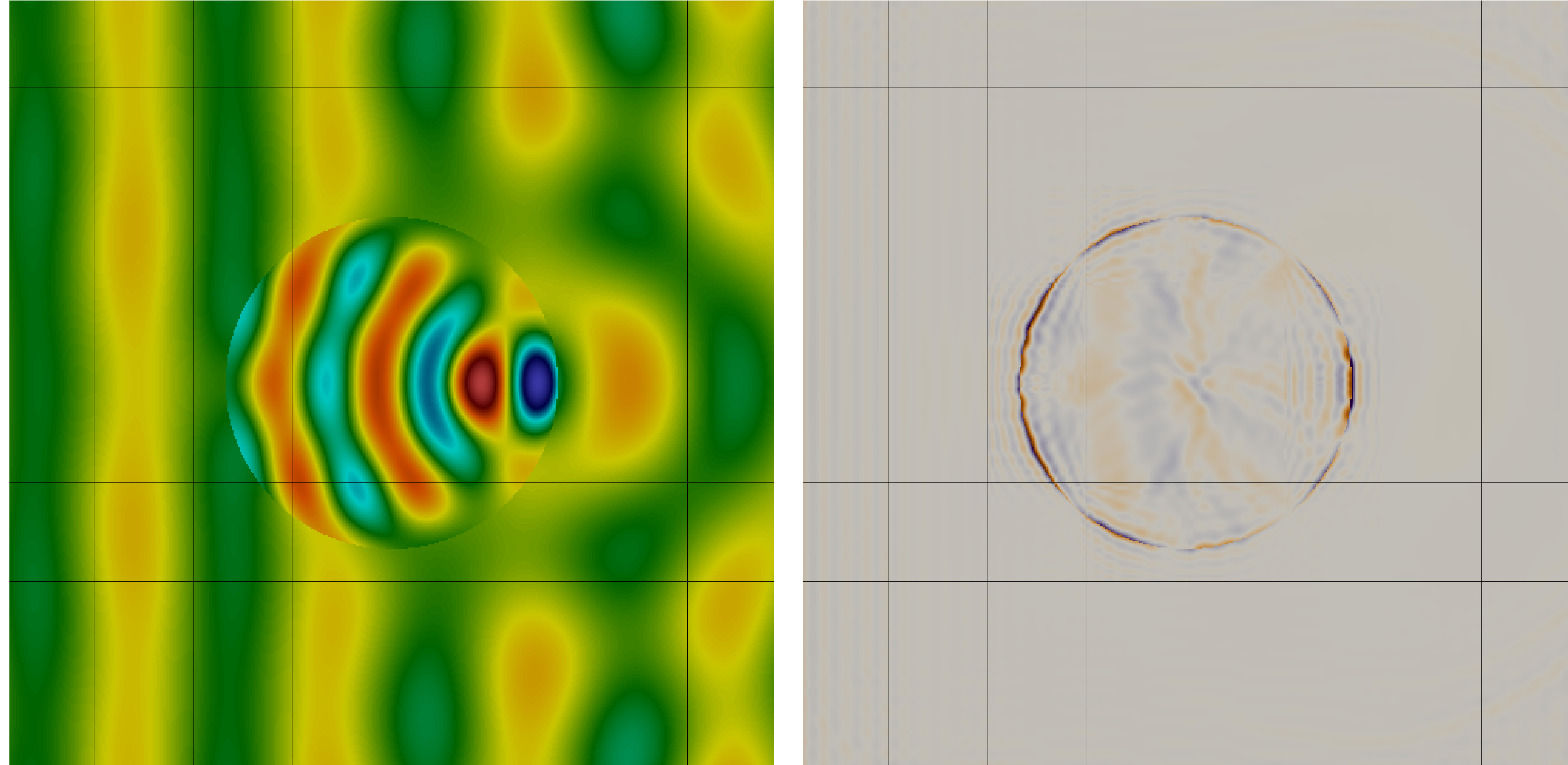
Illustration for the use of a generated geometry representation in an electrodynamic wave scattering setup
Scattering of a planar wave at a cylindrical object. The grid lines indicate the mesh of the DGFEM solver. For the numerical solution, a basis with a maximal polynomial degree of 15 is used. On the left, the reference solution is shown. On the right, the difference between the numerical solution and the reference can be seen for a de-aliasing by 32 points. The color scale for the difference is chosen with a range of +/- 10 % of the maximal amplitude in the reference.