
Spatiotemporal distribution and driving factors of atmospheric pollutants in the U-Chang-Shi urban agglomeration, Northwestern China
- Published
- Accepted
- Received
- Academic Editor
- Xinfeng Wang
- Subject Areas
- Environmental Sciences, Atmospheric Chemistry, Environmental Impacts, Spatial and Geographic Information Science
- Keywords
- Air pollutants, Spatiotemporal distribution, “U-Chang-Shi” urban agglomeration, HYSPLIT trajectory simulation
- Copyright
- © 2026 Chen et al.
- Licence
- This is an open access article distributed under the terms of the Creative Commons Attribution License, which permits using, remixing, and building upon the work non-commercially, as long as it is properly attributed. For attribution, the original author(s), title, publication source (PeerJ) and either DOI or URL of the article must be cited.
- Cite this article
- 2026. Spatiotemporal distribution and driving factors of atmospheric pollutants in the U-Chang-Shi urban agglomeration, Northwestern China. PeerJ 14:e20430 https://doi.org/10.7717/peerj.20430
Abstract
As a critical core node of the “Belt and Road” Initiative and a representative arid-zone urban agglomeration in Northwest China, the Urumqi-Changji-Shihezi (U-Chang-Shi) region faces severe air pollution, posing significant threats to ecological security and public health. Leveraging the 2000–2022 China High-Resolution Air Quality (CHAP) dataset and multi-source meteorological data, this study systematically investigates the spatiotemporal evolution of PM2.5, PM10, and ozone (O3) alongside their driving mechanisms. Results reveal distinct seasonal patterns: PM2.5 and PM10 concentrations peak in winter due to coal combustion emissions and unfavorable static meteorological conditions, while dropping below 30 µg/m3 in summer as photochemical reactions weaken. The Mann–Kendall (MK) trend test, combined with spatial-temporal analysis methods, elucidates the complex pollution dynamics. The U-Chang-Shi industrial belt acts as a pollution hotspot, with Dabancheng District exhibiting elevated PM10 levels attributed to pollutant transport and terrain effects. O3 pollution intensifies in spring and summer, surging post-2016 across regional cities, with Shihezi showing a 16.7% annual increase. Key drivers include unfavorable static meteorology and sparse vegetation for particulate pollutants, while precipitation (P) wet deposition enhances their removal. O3 production is modulated by potential evapotranspiration (PET) and wind speed (WIND), with high temperatures (T) accelerating photochemical reactions, although counteracted by particulate matter. Hybrid Single-Particle Lagrangian Integrated Trajectory Model (HYSPLIT) simulations indicate that Eurasian mid-latitude winter circulation and cross-border dust contribute to winter PM10 variability. Although the “coal-to-gas” project mitigated particulate pollution, its efficacy is constrained by Shihezi’s lagging industrial restructuring. This study provides critical insights for optimizing air pollution control strategies in ecologically vulnerable regions of Northwest China and arid-zone urban agglomerations under the Belt and Road Initiative, emphasizing the need for region-specific emission reduction measures and cross-border collaboration.
Introduction
The U-Chang-Shi urban agglomeration lies at the core of the northern slope of the Tianshan Mountain economic belt in Xinjiang, serving as a pivotal node in the Belt and Road Initiative. Although this area covers merely 3.8% of Xinjiang’s total land area, it concentrates over 40% of the region’s population and gross domestic product (GDP) (Li et al., 2002; see Fig. 1), with industrial activities characterized by high energy intensity and dominated by coal chemical and metallurgical sectors. The combination of a “trumpet-shaped” basin-like topography, frequent winter temperature inversions (Li et al., 2022), and episodic southeast dry hot wind events (Zheng et al., 2024) restricts atmospheric dispersion, prolonging pollutant residence time. Cross-border pollutant transport from Central Asia exacerbates the problem (Zhi et al., 2022; Duan et al., 2023).
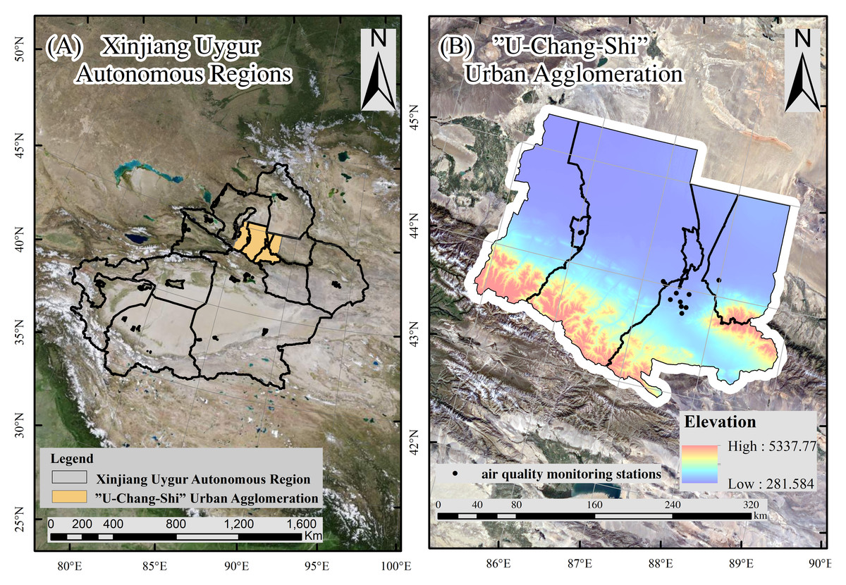
Figure 1: Geographical location and topography of the study area.
(A) Map of the Xinjiang Uygur Autonomous Region in northwest China, showing the administrative boundary (black outline) and the “U-Chang-Shi” Urban Agglomeration (orange-shaded region), comprising Urumqi, Changji, and Shihezi cities. (B) Detailed topographic map of the “U-Chang-Shi” Urban Agglomeration, with color gradients indicating elevation (red: high; blue: low; range: 281.584–5337.77 m). Black dots represent the locations of air quality monitoring stations used in this study. Both panels include a north arrow and scale bar for spatial reference.
Pollution control measures centered on the coal-to-gas conversion program successfully reduced PM10 by 26.1% in Urumqi during the winter of 2013–2014 compared to the pre-treatment period (2009–2011) (Li et al., 2016), yet their long-term effectiveness is constrained by lagging industrial restructuring and increasing ozone concentrations—growing at 4.6% annually since 2017 (Chu et al., 2021). Prior studies have examined spatial patterns (Min, 2020), meteorological influences (Li et al., 2022; Du et al., 2024), and pollution processes (Cao et al., 2023), but most analyses remain limited to short temporal spans (≤10 years) and rarely integrate socio-economic factors alongside environmental data.
In addition to air quality research, studies on carbon emission estimation models and influencing factors offer valuable insight into anthropogenic drivers of air pollution. Emission inventories compiled for stationary fossil fuel combustion sources in the U-Chang-Shi region show clear spatial heterogeneity in industrial and residential sectors (Wang et al., 2020; Yuan & Yang, 2020). Recent advances integrate input–output analysis, life-cycle assessment, and econometric modeling to link emission trends with economic growth, industrial structure, and technology adoption (Zhao et al., 2020; Zhou, Zhao & Yang, 2017). Combining these methods with high-resolution environmental datasets provides pathways for synergistic control of atmospheric pollution and greenhouse gas emissions—a policy direction increasingly emphasized in China’s dual-carbon goals.
Despite these advances, a critical gap remains: the lack of multi-decadal, high-resolution datasets capable of quantifying the coupled impacts of emissions, meteorology, and transboundary transport in arid urban clusters. Traditional monitoring networks provide partial temporal coverage, while most satellite-derived datasets suffer from cloud contamination or short time spans. The CHAP dataset (Wei et al., 2020; Wei et al., 2021a; Wei et al., 2021b; Wei et al., 2022) addresses this limitation by fusing MODIS multi-angle aerosol products, ground monitoring records, and high-quality emission inventories using AI-based algorithms. Covering 2000–2022 at one km resolution, CHAP achieves R2 > 0.67 in arid regions and incorporates recent algorithmic improvements that enhance accuracy for dust-laden conditions. The dataset enables consistent tracking of PM2.5, PM10, and O3 trends over two decades, providing a robust basis for evaluating policy effectiveness and climatic influences.
In this study, we leverage CHAP data in conjunction with multi-source meteorological datasets to analyze long-term spatial and temporal patterns of PM2.5, PM10, and O3 in the “U-Chang-Shi” agglomeration from 2000–2022. We investigate the interrelationships between pollutant dynamics, emission evolution—including insights from carbon emission modeling—and meteorological drivers, as well as cross-border transport impacts. Finally, we propose targeted measures emphasizing coordinated management of air pollutants and carbon emissions, thereby offering practical policy guidance for arid-zone megaregions under the Belt and Road framework.
Materials & Methods
Air pollutant data
Air pollutant concentrations (PM2.5, PM10, O3) were sourced from the CHAP dataset (2000–2022), developed through artificial intelligence-based fusion of MODIS multi-angle aerosol products with ground monitoring and emission inventory data (Wei et al., 2020; Wei et al., 2021a; Wei et al., 2021b; Wei et al., 2022). This 1-km resolution dataset, maintained by the University of Maryland research team and archived at the National Tibetan Plateau Science Data Center (NTPDC), addresses spatial gaps in conventional satellite retrievals.
Meteorological data
The 1-km resolution precipitation and temperature datasets (Peng et al., 2017a; Ding & Peng, 2020; Peng et al., 2019; Peng et al., 2017b) were constructed using Delta spatial downscaling methodology, integrating global climate products from the Climate Research Unit (CRU; 0.5° resolution) and WorldClim (high-resolution). These datasets underwent rigorous validation against observations from 496 meteorological stations across mainland China (including Hong Kong, Macao, and Taiwan) with demonstrated reliability. Spatial coverage excludes South China Sea islands but maintains continental continuity at 0.0083333° resolution (∼1 km).
Monthly potential evapotranspiration (PET) estimates were derived from China-specific 1-km temperature datasets (mean, min, max) archived at NTPDC (Peng et al., 2017a; Ding & Peng, 2020; Peng et al., 2019; Peng et al., 2021). Monthly PET was estimated using the Hargreaves formula. Daily wind speed data were obtained from NOAA’s National Centers for Environmental Information (NCEI). These station-based observations were then interpolated into a continuous national-scale raster dataset at a daily resolution using the Inverse Distance Weighting (IDW) algorithm, based on the geographic coordinates of the stations. Combining with administrative area of prefecture-level city crossing nationwide, after obtaining the statistic value of each station wind power density every day, then getting a day average velocity values of prefecture-level city in one day, month mean velocities got.
Normalized difference vegetation index data
The NDVI was derived from Landsat 5/7/8/9 imagery (2000–2022) via the Google Earth Engine platform. Annual maximum NDVI values were extracted at 30 m spatial resolution after preprocessing and smoothing, with outputs stored in GeoTIFF format (Didan, 2015).
Coefficient of determination
The coefficient of determination (R2) quantifies the proportion of variance in observational data explained by model simulations, and is defined as: (1) where (yi) denotes the in-situ measurements from observational stations (PM2.5, PM10, O3), represents the CHAP dataset, is the mean of observational data, and n is the sample size. The numerator, residual sum of squares (RSS), measures the discrepancy between the CHAP dataset and observations, while the denominator, total sum of squares (TSS), reflects the natural variability of observations.
Spearman correlation analysis
Spearman correlation analysis is a non-parametric statistical method for quantifying monotonic relationships between variables, which centers on calculating correlations from variable rank order (rather than raw values) and is applicable to non-linear or non-normally distributed data. The method effectively eliminates the effects of outliers and data distribution patterns by converting the data into rank series, and is able to robustly reveal trend consistency among variables (Spearman, 1904). Given its robustness to non-normal data and outliers, Spearman correlation analysis is widely applied in environmental science to uncover non-linear relationships between diverse geographical factors (Biswas, Chatterjee & Chakraborty, 2020; Zhang et al., 2015).
Within this research, the Spearman rank correlation coefficient (ρ) was employed to measure the magnitude and trend of monotonic relationships between PM2.5, PM10, O3 concentrations and meteorological parameters, respectively. The statistical significance was set at a p-value threshold of less than 0.05. The analyses were carried out using SPSS software, and the visualization was completed through Origin. (2) where: R is the correlation coefficient; Xi is the pollutant concentration in month i, µg/m3; is the average of the pollutant concentration in all months; Yi is the value of meteorological elements in month i (when Y is precipitation, temperature, PET, wind speed, the unit is mm, °C, mm, m/s, respectively); is the average value of meteorological elements (the unit is the same as the above); N is the time series length (2000–2022).
Grey relational analysis
Grey relational analysis (GRA) quantifies inter-factor associations by evaluating geometric similarity between data sequences (i.e., the proximity of curve variation trends), where higher relational grades indicate more consistent dynamic changes between paired sequences (Deng, 1982). In this study, grey relational analysis was employed to assess dynamic correlations between pollutant concentrations and key meteorological factors. The analytical procedure involved three sequential steps: first, original data underwent normalization to eliminate dimensional discrepancies. Subsequently, grey relational grades were computed using MATLAB (The MathWorks, Natick, MA, USA) with a distinguishing coefficient set at 0.5. The resultant ranking of relational grades facilitated identification of dominant meteorological factors, which were then cross-validated against correlation analysis results. This methodological implementation strictly adhered to standardized protocols in grey system theory while maintaining compatibility with conventional statistical approaches.
(3) (4) where ζi(k) is the grey relational coefficient; ri is the degree of grey relational grade. y(k) is the normalized parameter value; xi(k) is the normalized comparison value, i is the number of comparison arrays (i = 1, 2...n), and k is the number of indicators for each comparison object (k = 1,2, …, m); ρ is the discrimination coefficient, which usually takes the value of 0.5; based on the results of previous research (Liu, Zhang & Li, 2018), the interval of the correlation value is divided into the degree of strength of the correlation, with [1, 0.8] as strong, (0.8, 0.6) as stronger, (0.6, 0.4) as moderate, (0.4, 0.2) as weaker, and [0.2, 0) as weak.
The Theil–Sen estimator
The slope n of pairs of data points was estimated using the Theil–Sen (TS) estimator (Sen, 1968; Theil, 1992), which is given by Eq. (5). (5) where xi and xj are data values at times ti and tj(i > j), respectively. The slope that was calculated by the TS estimator is a robust estimate of the magnitude of a trend, and the use of the TS slope provides the special benefit of the rejection of inter-annual variability (Neeti & Eastman, 2011). This study employed the MK trend test, which assesses the similarity level between two sets of rankings assigned to the same set of objects. As indicated in references (Kendall, 1938; Hirsch, Slack & Smith, 1982; Valz & McLeod, 1990; Lanzante, 1996), this test relies on the number of inverted object pairs needed to convert one ranking order into the other. The data were first ranked according to the temporal sequence. Subsequently, each data point was sequentially taken as a reference point and compared with all subsequent data points in the time series, as described in reference (Douglas, Vogel & Kroll, 2000). A key challenge in applying time series analysis effectively lies in distinguishing between a genuine change in a remotely sensed variable (such as a vegetation index) and the presence of scene noise (such as smoke or cloud contamination), as noted in reference (Neeti et al., 2012).
The Mann–Kendall trend test
The Mann–Kendall (MK) trend test is designed to determine the existence of trends for each time scale independently. This test involves calculating the MK statistic (S) using the formulas in Eqs. (5) and (6), as cited in references (Dietz & Killeen, 1981; De Beurs & Henebry, 2004; De Jong et al., 2011; Sobrino & Julien, 2011).
(6) (7)
Here, xj and xk denote the data points at time j and k(j > k) respectively, and n represents the total number of data points. However, to statistically measure the significance of the trend, it is essential to calculate the probability associated with the statistic S and the sample size n. When n ≥ 10, the statistic: S approximately follows a normal distribution, with its mean and variance defined by Eq. (7), as stated in references (De Beurs & Henebry, 2004; An, 2007). (8) (9)
In this context, S represents the test statistic, Z is the standardized test statistic, and n signifies the length of the time series. At a specified significance level ɛ, when |F| > F1-ɛ/2, the time series data show a distinct change trend. In this study, temporal trends are considered significant when F < −1.96 or F > 1.96. The Z statistic follows the standard normal distribution: a positive value implies an upward trend, while a negative value indicates a downward trend.
HYSPLIT trajectory simulation analysis
HYSPLIT is a commonly used model for analyzing pollutant distribution laws and transportation in the atmosphere, which is constructed by the NOAA of the United States (Draxler & Hess, 1998). The model adopts Lagrangian particles diffusing and Eulerian grids dispersing methods to realize three-dimensional air flow paths and quantify pollutants’ diffusion, dilution, wet dry deposition etc., based on trajectory calculation engine and diffusion prediction module, which can perform analysis from an hour’s scale up to seasons, taking meteorological data at different scales. In this experiment, global forecast meteorology data driven model with lateral space interval 0.25 × 0.25° and vertical layer stratification number 38, describing mid-latitude atmospheric circulation conditions in Eurasia under winter weather, was selected. There are release height AGL such as 500 m green color, 1,000 m blue color, 3,000 m red color in our experiments for two-way propagation processes between seven days’ back tracing and predictive steps further along (Rolph, Stein & Stunder, 2017).
The overall research design and the integrated methodological workflow employed in this study are summarized in Fig. 2. This schematic illustrates the sequential process from multi-source data acquisition and preprocessing to the application of statistical analyses and models, culminating in the final results and conclusions.
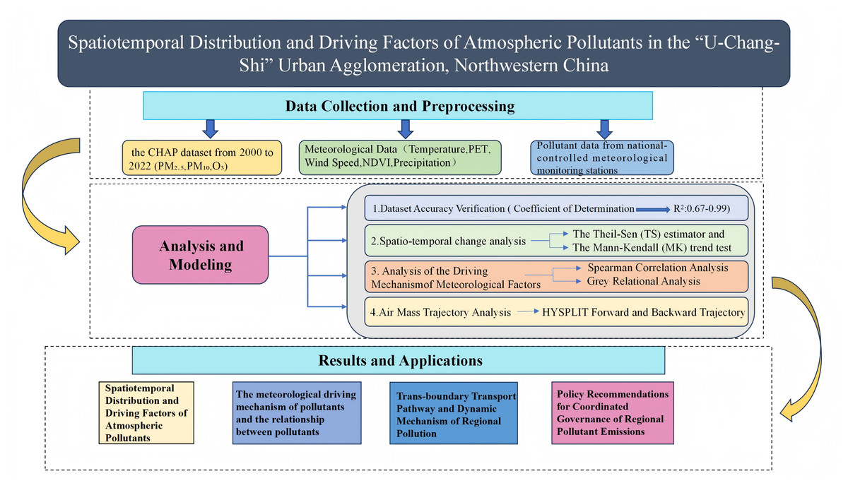
Figure 2: Research framework.
The flowchart outlines the integrated methodology, which consists of three main phases: (1) Data Collection and Preprocessing, involving the acquisition of long-term (2000–2022) air pollutant concentrations (PM2.5, PM10, and O3) from the ChinaHighAirPollutants (CHAP) dataset, meteorological data (temperature, potential evapotranspiration (PET), wind speed, NDVI, and precipitation), and validation data from national-controlled monitoring stations; (2) Analysis and Modeling, which includes dataset accuracy verification (using the Coefficient of Determination, R2), spatiotemporal trend analysis (using the Theil–Sen estimator and Mann–Kendall test), analysis of driving mechanisms (using Spearman correlation and Grey Relational Analysis), and air mass trajectory analysis (using the HYSPLIT model); and (3) Results and Applications, aimed at generating policy-relevant insights on pollutant distributions, meteorological drivers, trans-boundary transport pathways, and regional coordinated governance strategies. Arrows indicate the sequential flow and integration of analytical steps.
Results
Dataset accuracy verification
This study takes the U-Chang-Shi urban agglomeration as the study area, and there are 12 state-controlled stations in this area, namely, seven monitoring stations in Urumqi, seven monitoring stations in Xinjiang Academy of Agricultural Sciences farms, monitoring stations, railway bureau, 31st middle school, 74th middle school, Midong District Environmental Protection Bureau and fee collection office, three monitoring stations in Changji Prefecture, two monitoring stations in Sunshine School and Aiqing Poetry Hall, and two monitoring stations in Shihezi City, and the Agricultural Water Building in Wujiaqu. Three monitoring stations in Changji Prefecture; two monitoring stations in Shihezi City, at the Sunshine School and the Aiqing Poetry Hall; and the Agricultural and Water Building in Wujiaqu, We first validated this dataset by linearly fitting the PM2.5 dataset for December 2018, January 2019, and February 2019, as well as July, August, and September 2019, to the air quality values provided by the China Air Quality Online Monitoring and Analysis Platform (https://www.cnemc.cn/). Prior to the fitting, we sampled and extracted the values of the Tif images of the dataset at the coordinates of the 12 state-controlled stations in the study area using Arcgis software. From the fitting results of each station (Fig. 3), the R2 values range from 0.67 to 0.99.
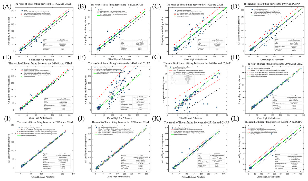
Figure 3: Linear fitting results between CHAP datasets and ground-based air quality monitoring data.
(A–L) Shows the relationship between a specific CHAP product (1490A, 1491A, 1492A, 1493A, 1494A, 1496A, 2690A, 2691A, 2692A, 2709A, 2710A, 2711A) and corresponding measurements from air quality monitoring stations. Blue dots represent observed values from monitoring stations. The solid blue line indicates the linear fit of “A” station data; the red dashed line denotes the 95% prediction band for “A” station. The green dashed line represents the 95% prediction band for “B” station; the solid green line shows the linear fit of “B” station data. Each subplot includes statistical parameters such as equation, intercept, slope, residual sum of squares, Pearson’s r, R-square (COD), and adjusted R-square to evaluate the goodness-of-fit.
This R2 range can indicate that the independent variable explains the dependent variable to a high degree and the fitting effect is significant. It can be proved that the CHAP dataset of the University of Maryland has a good applicability within the U-Chang-Shi region in the interior of the arid zone.
Monthly and seasonal spatial distribution characteristics of air pollutants
As shown in Figs. 4 and 5, observational data indicate a clear seasonal pattern in O3 concentrations in the U-Chang-Shi region. The monthly mean concentrations increase significantly from late spring to summer (April–August), from approximately 92.15 µg/m3 in April to a yearly maximum of 144.86 µg/m3 in July and 145.27 µg/m3 in August. This represents an overall increase of nearly 58% from April to midsummer. In contrast, O3 concentrations in autumn and winter seasons (September–December) remain much lower, with monthly means dropping from 89.47 µg/m3 in September to 57.29 µg/m3 in November and as low as 14.02 µg/m3 in December, representing more than an 84% decline compared to the summer peak.
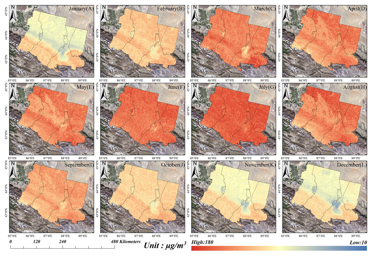
Figure 4: Monthly spatial distribution of O3 concentrations in the “U-Chang-Shi” Urban Agglomeration from January to December.
(A–L) Represents one month, with color gradients indicating O3 levels ranging from low (10 µg/m3, blue tones) to high (180 µg/m3, red tones). The black arrow indicates north direction, and the scale bar at the bottom left denotes a distance of 480 kilometers for spatial reference. These maps collectively illustrate the temporal and spatial patterns of O3 concentration across the region.
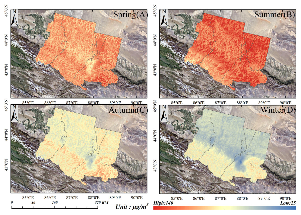
Figure 5: Seasonal spatial distribution of O3 concentrations in the “U-Chang-Shi” Urban Agglomeration.
(A–D) Represent spring, summer, autumn, and winter, respectively. The color gradient indicates O3 concentration levels, ranging from low (25 µg/m3, blue tones) to high (140 µg/m3, red tones). The black arrow in the top-left corner of each subplot indicates north direction, and the scale bar at the bottom left denotes a distance of 320 km for spatial reference. These maps collectively illustrate the seasonal variations in O3 spatial patterns across the region.
Spatially, the high-concentration zones (above 130 µg/m3) in summer cover the majority of the region, particularly in industrial areas with intensive NOx and (Volatile Organic Compounds (VOC) emissions. Winter maps show extensive low-concentration zones (below 30 µg/m3) dominated by blue and light-yellow areas. The most polluted period appears in summer, followed by spring, while autumn and winter exhibit the lowest levels.
The spring transitional period (March–May) shows a steady increase (from 84.37 µg/m3 in March to 97.84 µg/m3 in May, a rise of ∼16%). Once autumn temperatures begin to drop (September–November), mean O3 concentrations fall sharply (>35% within two months).
Overall, the intra-annual fluctuation in O3 concentration within this region is substantial, ranging from 14 µg/m3 to 145 µg/m3.
These large variations indicate that multiple factors influence air quality: in addition to local industrial production, transportation emissions, and human activities, long-range transport of pollutants also contributes to the observed O3 levels. This seasonal pattern is consistent with earlier findings (An, 2007), confirming that O3 pollution reaches its maximum intensity in summer, moderate in spring, and minimal in autumn–winter periods. The spring transitional rise is probably due to gradually rising temperatures and increasing VOC emissions. The rapid autumn decline is driven by the reduction of photochemical reaction rates.
The monitoring results (Figs. 6 and 7) show that the winter season (December–February) is the most polluted period in the U-Chang-Shi region. In January, the mean concentration at Changji reached 171 µg/m3, representing the highest recorded value. High-value contamination zones (>150 µg/m3) appear in western Shihezi, central Urumqi, northwestern Changji, the northern part of Shawan, and the southern part of Wujiaqu during winter.
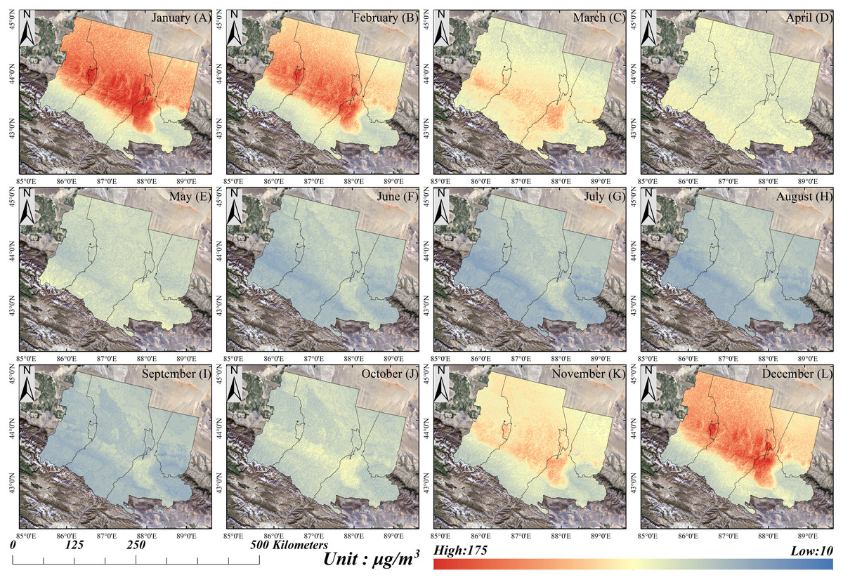
Figure 6: Monthly spatial distribution of PM2.5 concentrations in the “U-Chang-Shi” Urban Agglomeration from January to December.
(A–L) Represents one month, with color gradients indicating PM2.5 levels ranging from low (10 µg/m3, blue tones) to high (175 µg/m3, red tones). The black arrow in the top-left corner of each panel indicates north direction, and the scale bar at the bottom left denotes a distance of 500 km for spatial reference. These maps collectively illustrate the temporal and spatial patterns of PM2.5 concentration across the region.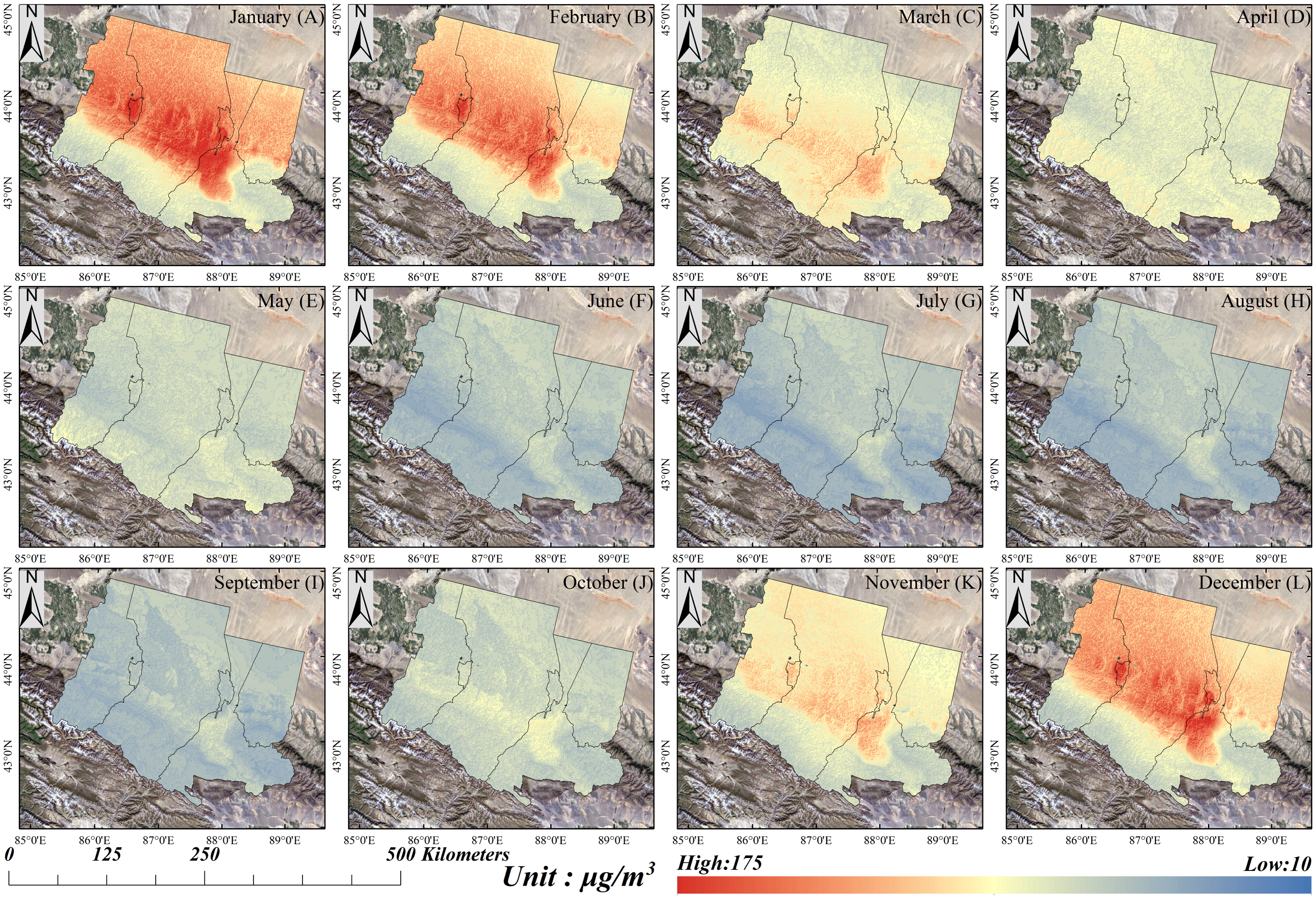
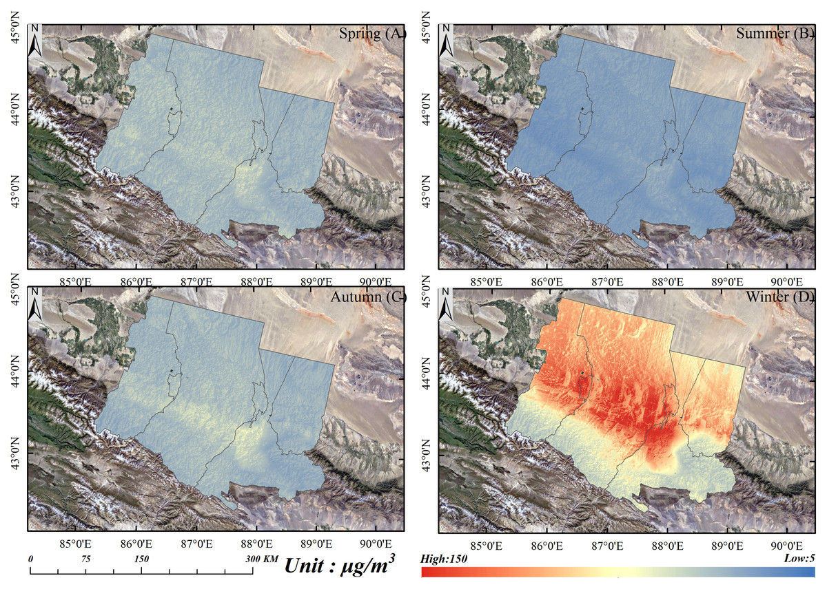
Figure 7: Seasonal spatial distribution of PM2.5 concentrations in the “U-Chang-Shi” Urban Agglomeration.
(A–D) Represent spring, summer, autumn, and winter, respectively. The color gradient indicates PM2.5 concentration levels, ranging from low (5 µg/m3, blue tones) to high (150 µg/m3, red tones). The black arrow in the top-left corner of each subplot indicates north direction, and the scale bar at the bottom left denotes a distance of 300 km for spatial reference. These maps collectively illustrate the seasonal variations in PM2.5 spatial patterns across the region.
For particulate matter, spring is the cleanest season: may recorded a mean concentration of 31.52 µg/m3, which is about 40% lower than March (52.67 µg/m3). Summer concentrations are mostly under 30 µg/m3—over 80% lower than the January peak. Autumn values gradually rebound from 30.15 µg/m3 in September to 46.38 µg/m3 in November, an increase of nearly 50%. Across the year, PM2.5 fluctuates between 14 and 171 µg/m3.
Such seasonal variation is directly linked to meteorological conditions, emission intensities, and the effect of topography in trapping pollutants during the stagnant winter period. The winter peaks are influenced by heating activities and unfavorable atmospheric dispersion, while the low concentrations in summer are aided by stronger mixing and precipitation scavenging.
Figures 8 and 9 show that PM10 concentrations also peak during winter, with the highest value (225 µg/m3) measured in Urumqi in January, and the lowest value (43 µg/m3) in July. Spring mean concentrations decreased by 13.53% from March to May, while autumn increased by 17.75% from September to November. The seasonal sequence is winter > spring > autumn > summer. During spring, an unusual high-value PM10 zone is visible at the border between southeastern Urumqi and Turpan, while most of the rest of the region has moderate levels.
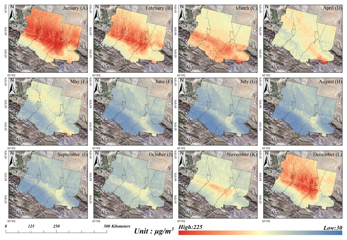
Figure 8: Monthly spatial distribution of PM10 concentrations in the “U-Chang-Shi” Urban Agglomeration from January to December.
(A–L) Represents one month, with color gradients indicating PM10 levels ranging from low (30 µg/m3, blue tones) to high (225 µg/m3, red tones). The black arrow in the top-left corner of each panel indicates north direction, and the scale bar at the bottom left denotes a distance of 500 km for spatial reference. These maps collectively illustrate the temporal and spatial patterns of PM10 concentration across the region.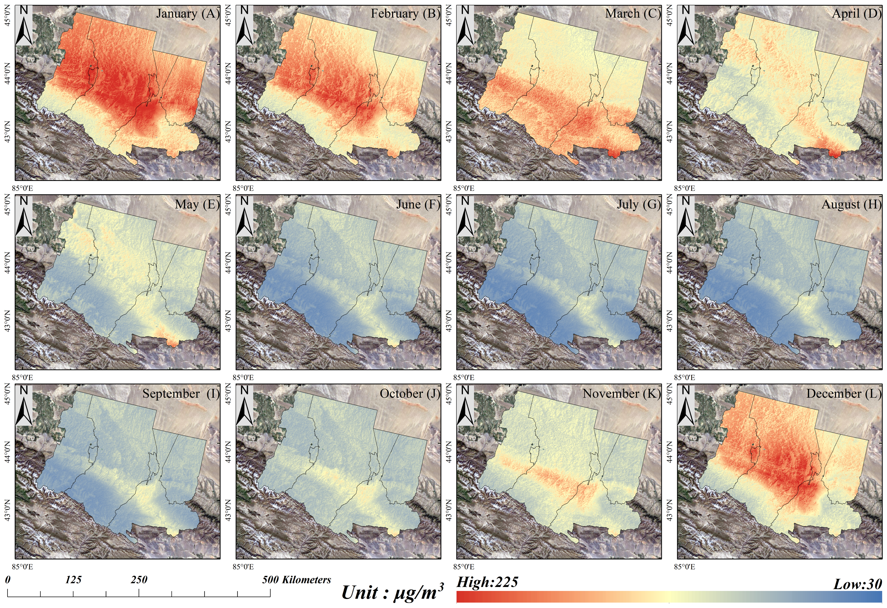
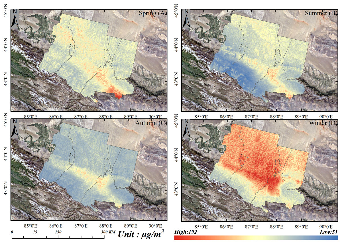
Figure 9: Seasonal spatial distribution characteristics of PM10 concentration.
The seasonal spatial distribution of PM10 concentration in a study area. It contains four subplots corresponding to spring, summer, autumn, and winter, respectively. The color gradient represents PM10 concentration levels, with a range from low (51 µg/m3, blue tones) to high (192 µg/m3, red tones), and the unit is µg/m3. The black arrow in the top - left corner of each subplot indicates the north direction, and the scale bar at the bottom left (labeled “300 KM”) serves as a spatial scale reference. These maps collectively illustrate the seasonal variations in the spatial distribution of PM10.
The higher PM10 levels in spring and autumn compared to PM2.5 are due to the significant contribution of coarse particles, including dust events and soil particles. The distinctive southeastern Urumqi–Turpan high-value zone is likely linked to local topography, prevailing wind directions, and dust source proximity.
Annual concentration trends and statistical characteristics of air pollutants
Figure 10 presents a comprehensive analysis of the spatiotemporal evolution of PM2.5 and PM10 concentrations in the “U-Chang-Shi” region from 2000 to 2022. Figure 10A illustrates the interannual variability of PM2.5 concentrations in the “U-Chang-Shi” region from 2000 to 2022. Over this 22-year period, annual mean PM2.5 levels exhibited a fluctuating decline, decreasing from 50.18 µg/m3 in 2000 to 40.26 µg/m3 in 2022 (17.92% reduction). Concurrently, PM10 concentrations followed a similar trajectory, declining from 102.33 µg/m3 to 77.67 µg/m3 (24.09% reduction; see Fig. 10B). Notably, both pollutants displayed synchronized temporal patterns, with peaks observed in 2012 followed by substantial reductions post-2015.
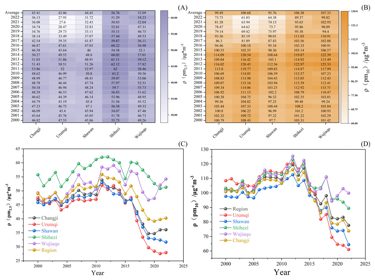
Figure 10: Interannual trends and annual mean concentration variation characteristics of PM2.5 and PM10.
(A) Heatmap of annual mean PM2.5 concentrations (µg/m3) across five cities (Changji, Urumqi, Shawan, Shihezi, and Wujiaqu). Color intensity scales with concentration magnitude, ranging from ∼30 µg/m3 (lightest) to ∼60 µg/m3 (darkest). (B) Heatmap of annual mean PM10 concentrations (µg/m3) for the same five cities. The color gradient represents concentrations from ∼60 µg/m3 (lightest) to ∼130 µg/m3 (darkest). (C) Interannual variation of PM2.5 concentrations. Trend lines are colored by city: Changji (gray), Urumqi (red), Shawan (blue), Shihezi (green), Wujiaqu (purple). The gold line represents the regional average. (D) Interannual variation of PM10 concentrations, following the same color scheme and location correspondence as panel (C). All panels share the same horizontal axis representing the study period from 2000 to 2022. Vertical axes in (C) and (D) show concentration values in µg/m3.
City-specific analyses revealed heterogeneous trends from 2000 to 2022. PM2.5 and PM10 concentrations decreased significantly in Urumqi (by 41.21% and 43.72%, respectively), Shawan (30.83% and 34.10%), and Changji (22.83% and 26.83%). In contrast, the declines in Shihezi were much smaller, with a PM10 reduction of only 4.49%. Notably, Wujiaqu was an exception, experiencing a 10.09% increase in PM2.5 with its PM10 level remaining largely stable (a slight decrease of 1.57%).
The temporal dynamics of PM2.5 from 2000 to 2022 exhibited three distinct phases (Fig. 10C): a period of irregular increase until 2012, a sharp decline from 2013 to 2015, and a steady decrease following a brief rebound in 2016. Wujiaqu City constituted an exception to this regional pattern, showing a continuous upward trend. Similarly, PM10 concentrations followed a comparable trajectory, characterized by a primary peak between 2012 and 2014, a decrease around 2017, and a sustained decline thereafter (Fig. 10D).
From the perspective of Urumqi’s regional air pollution and environmental management, 2012 was the peak of regional pollutant concentration average, and the beginning of air pollution and environmental management focus. “Coal to gas” project began to implement, Urumqi City in six months to complete the transformation of 12,900 tons of steam tons, the particulate matter (PM2.5, PM10) can also be seen in the graph of a significant decline. In the process of pollution management, 2016, 2017 particulate matter (PM2.5, PM10) appeared in the concentration value of the phenomenon of a small rebound after the timely containment, and strong, effective management of pollutants, and after 2020 leveled off. This shows that the remediation of the atmospheric environment has achieved gradual results.
Figure 11 illustrates the contrasting temporal dynamics of O3 concentrations across the study region. As summarized in the heatmap (Fig. 11A), O3 levels remained relatively stable from 2000 to 2016, with annual variations ranging from −0.14% to +0.6%. During this period, Shihezi and Wujiaqu consistently exhibited lower baseline concentrations compared to other urban centers. A notable regime shift occurred after 2016, as clearly depicted in the temporal trend analysis (Fig. 11B), marked by accelerated growth rates of 4.2–4.6% annually during 2017–2022. The trend graph particularly highlights anomalous spikes in 2017, with Urumqi and Shihezi experiencing increases of 7.1% and 16.7% respectively—a pattern potentially linked to extreme thermal episodes or intensified industrial activity. Although a transient decline emerged in 2020, the post-2016 upward trajectory remained unaltered, with all cities exceeding 7% annual growth during peak phases. The persistent growth momentum observed after 2016, especially the rapid increase starting in 2017 shown in Fig. 11B, appears largely unabated. This trend may be attributed to the surge in industrial emissions in recent years. For instance, the commissioning of the chemical park in Shihezi City in 2017, as reflected in the notable 16.7% concentration increase for that year, provides a plausible explanation for the observed spatial–temporal pattern.
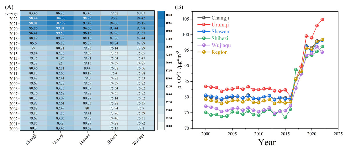
Figure 11: Map of O3 interannual trend (A) and annual mean concentration variation characteristics (B).
(A) Temporal variation of O3 concentrations (µg/m3) across five urban areas and the regional average from 2000 to 2025. Trends are indicated by distinct colored lines: Changji (gray), Urumqi (red), Shawan (blue), Shihezi (green), Wujiaqu (purple), and the regional average (gold). Note: data from 2023 to 2025 represent projected or extrapolated values. (B) Heatmap of annual mean O3 concentrations (µg/m3) for the five cities from 2000 to 2022. Color intensity corresponds to concentration magnitude, ranging from ≈ 70 µg/m3 (lightest) to ≈ 105 µg/m3 (darkest), as quantified in the adjacent color bar.Together, these panels highlight both long-term trends and fine-scale spatial heterogeneity in O3 levels across the region.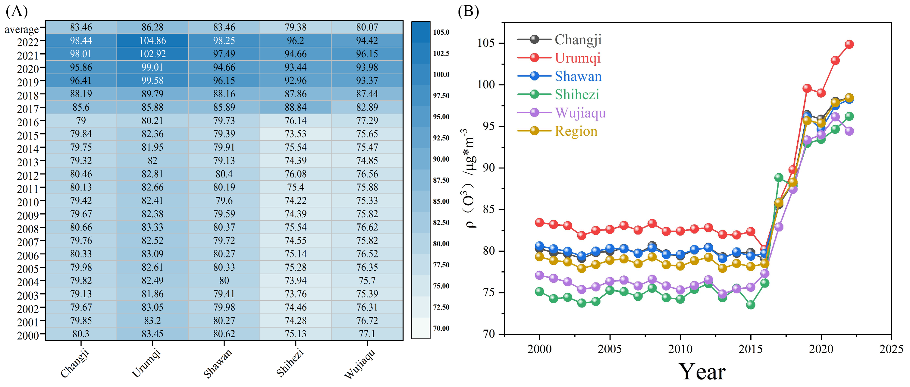
Spatial distribution patterns of multi-year average pollutant concentrations
Figure 12A reveals pronounced spatial heterogeneity in multi-year average PM2.5 concentrations (2000–2022) across the “U-Chang-Shi” region, with values ranging from a minimum of 30.70 µg/m3 in the southern mountainous areas to a maximum of 75.90 µg/m3 in Urumqi’s metropolitan core. High-value zones (>70 µg/m3) form a contiguous east–west corridor stretching from Urumqi through Changji Jundong to Shihezi, corresponding to regions of dense population, intensive industrial activity, and heavy traffic emissions. Areas with medium concentrations (50–65 µg/m3) are primarily located in northwestern Changji, Shawan, and Wujiaqu, while low-value zones (<40 µg/m3) are distributed mainly in peripheral natural landscapes, particularly the high-altitude southern mountains where cleaner air is maintained due to strong atmospheric dispersion and limited anthropogenic sources.
Figure 12: Spatial distribution of multi - year average concentrations of PM2.5 and PM10.
The spatial distribution of multi-year average concentrations of PM2.5. and PM10, containing two subplots: (A) PM2.5 Annual Average Concentration Spatial Distribution Map . The color gradient represents PM2.5 concentration levels, ranging from low (30.7 µg/m3, blue tones) to high (75.9 µg/m3, red tones), with the unit being µg/m3. The black arrow in the top-right corner indicates the north direction, and the scale bar at the bottom (labeled “0–180 KM”) provides a spatial scale reference. (B) PM10 Annual Average Concentration Spatial Distribution Map. The color gradient represents PM10 concentration levels, ranging from low (71.80 µg/m3, blue tones) to high (142.82 µg/m3, red tones), with the unit being µg/m3. The black arrow in the top-right corner indicates the north direction, and the scale bar at the bottom (labeled “0–180 KM”) provides a spatial scale reference. Collectively, the figure depicts the spatial variation of multi-year average PM2.5 and PM10 concentrations across the study area.
This stark north–south gradient reflects the combined influence of topography—with mountain ranges acting as barriers to pollutant transport—and land-use patterns, where urban-industrial belts generate persistent PM2.5 hotspots, contrasting with the low-emission natural terrain in the south.
Figure 12B illustrates the multi-year (2000–2022) average spatial distribution of PM10 in the “U-Chang-Shi” region, with concentrations ranging from a minimum of 71.80 µg/m3 in the southern mountainous areas to a maximum of 142.82 µg/m3 in the core urban zone of Urumqi. High-concentration zones (>130 µg/m3) form a continuous pollution belt encompassing Urumqi, Shihezi, and Wujiaqu, and extending to the Urumqi–Turpan border. Surrounding areas show a gradual decrease in concentration toward the south of the Wuquan Canal, with markedly lower values (<85 µg/m3) south of the Shawan Mountain range.
A particularly notable anomaly is evident in the southeastern Urumqi mountain area, where PM10 levels remain unexpectedly high (∼125–135 µg/m3), a feature absent in other particle size distribution maps. This anomaly is possibly related to complex topography—alternating high valleys and low hollows with vegetation (e.g., poplar forests) and sulfur-rich geological zones. Under such terrain conditions, airflows shift abruptly, especially near nightfall, when cold air descends the slopes and accumulates in valley floors, forming a stable stratification that traps particulates.
This persistent spatial pattern—urban-industrial hotspots contrasting against cleaner high-altitude southern regions—highlights the combined influence of anthropogenic emissions and terrain-driven atmospheric processes in shaping PM10 distributions.
Figure 13 shows that, compared to PM2.5 and PM10, elevated O3 concentrations occupy a more extensive and clearly defined spatial range across the “U-Chang-Shi” region, with values ranging from 62.70 µg/m3 to a maximum of 96.50 µg/m3. The highest O3 levels are concentrated in the southeastern part of Urumqi—particularly in areas adjacent to Turpan City—and the southern part of Changji City, where average concentrations exceed 90 µg/m3.
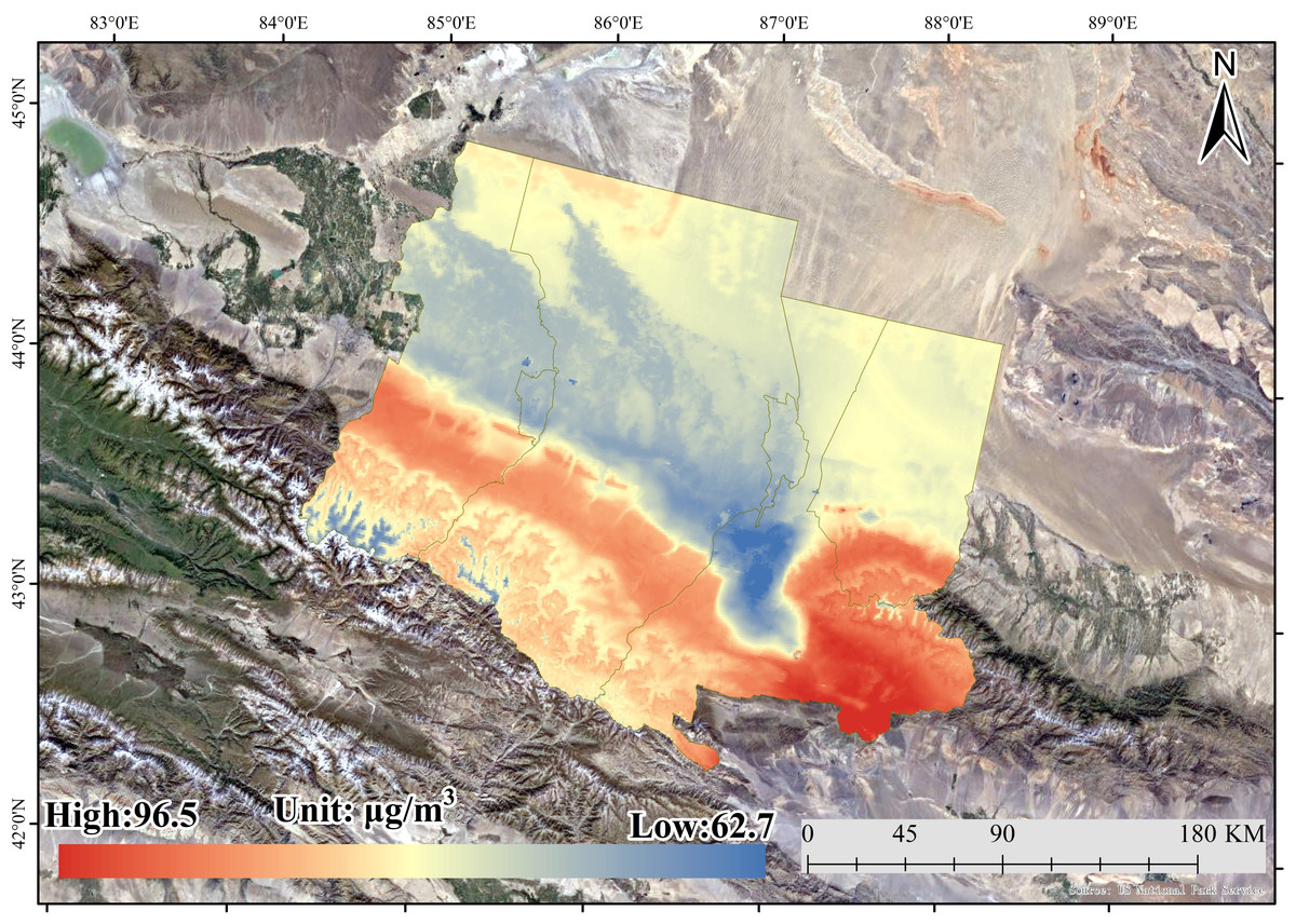
Figure 13: Spatial distribution of O3 multi-year averages.
The spatial distribution of annual average ozone (O3) concentration. The color gradient represents O3 concentration levels, ranging from low (62.7 µg/m3, blue tones) to high (96.5 µg/m3, red tones), with the unit being µg/m3. The black arrow in the top - right corner indicates the north direction, and the scale bar at the bottom right (labeled “0–180 KM”) provides a spatial scale reference for the study area. This map illustrates the spatial variation of annual average O3 concentration across the region.
Medium-value regions (approximately 75–85 µg/m3) are typically adjacent to these hotspots, extending along the southwestern mountainous zones near the northern foothills of the Tianshan Mountains. These areas present sharp concentration boundaries following the topographic transitions in the mountainous terrain.
In contrast, low-value areas (<70 µg/m3) are primarily located in the central “U-Chang-Shi” region, including the main urban core of Urumqi, where complex interactions between atmospheric dynamics and precursor emissions limit O3 accumulation compared to surrounding elevated zones.
The spatial gradient—high values in the topographically elevated southern margins and low values in central depressions—reflects the influence of terrain-driven meteorological processes (e.g., enhanced photochemical activity in high-altitude, sun-exposed slopes) combined with local precursor distribution patterns.
MK trend of air pollutants
Overall, the TS Slope values (Fig. 14B) exhibit a high consistency with the MK-Z values of PM2.5 (Fig. 14A) in terms of spatial distribution. The central and northern regions show a larger slope, and the MK-Z is significantly positive (|Z| ≥ 1.96, corresponding to p < 0.05), reflecting a significant increasing trend in PM2.5 concentration, with the maximum annual increase reaching up to 4.04 µg m−3 yr−1. In the southern and southwestern mountainous areas, the slope is negative and the MK-Z is significantly negative (p < 0.05), indicating a significant decreasing trend, with the maximum annual decline reaching −4.80 µg m−3 yr−1. Some marginal and central areas show Z values close to 0 (—Z—< 1.96, corresponding to p ≥ 0.05), indicating that the change trends are statistically insignificant. Notably, the MK-Z values and TS Slope values in the Uga District and Shihezi City are both at a high level, and the significance test (p < 0.05) reflects that PM2.5 concentrations in these areas have significantly increased in recent years.
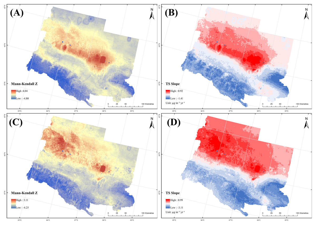
Figure 14: Per-Pixel Mann–Kendall Z values and Theil–Sen (TS) slope values of PM2.5 and PM10 from 2000 to 2022.
The per-pixel trend analysis results for PM2.5 and PM10 concentrations from 2000 to 2022, using the Mann–Kendall test and Theil–Sen (TS) estimator, with four subplots: (A) Mann–Kendall Z value map for PM2.5. The color gradient (ranging from low: −4.80 to high: 4.04) indicates the significance of PM2.5 temporal trends (positive Z values denote statistically significant increasing trends, negative Z values represent significant decreasing trends, and values near zero imply non-significant trends). (B) TS slope map for PM2.5. The color gradient (ranging from low: −1.41 to high: 0.92 µg m−3 yr−1) reflects the magnitude and direction of PM2.5 concentration change over time (positive TS slope values signify increasing trends, negative values indicate decreasing trends). (C) Mann–Kendall Z value map for PM10. The color gradient (ranging from low: −4.25 to high: 3.11) indicates the significance of PM10 temporal trends (interpreted as for PM2.5 in (A)). (D) TS slope map for PM10. The color gradient (ranging from low: −3.11 to high: 0.99 µg m−3 yr−1) reflects the magnitude and direction of PM10 concentration change over time (interpreted as for PM2.5 in (B)). In all subplots, the black arrow indicates the north direction, and the scale bar (labeled “0–100 Kilometer”) provides a spatial reference for the study area.
The TS Slope values (Fig. 14D) and MK-Z values of PM10 (Fig. 14C) exhibit broadly consistent spatial patterns. In the central–northern part of the region, both TS Slope values are positive and MK Z values are significantly positive (|Z| ≥ 1.96, p < 0.05), indicating a statistically significant increasing trend, with annual growth rates reaching up to 3.11 µ g m−3 yr−1. In the southern and southwestern mountainous areas, TS Slope values are negative and MK Z values are significantly negative (p < 0.05), reflecting a significant decreasing trend, with the largest decline reaching −4.25 µg m−3 yr−1. In some marginal and central areas, MK Z values are close to zero (|Z| < 1.96, p ≥ 0.05) and TS Slope values are near zero, suggesting statistically insignificant long term changes. Notably, Wujiaqu City and Shihezi City have both high TS Slope values and significantly positive MK Z values (p < 0.05), highlighting a pronounced and statistically significant upward trend in these areas.
Figure 15 presents the spatial heterogeneity in both the statistical significance and magnitude of O3 concentration trends across the study region from 2000 to 2022. As shown in Fig. 15A, the per-pixel MK-Z values analysis reveals a distinct north–south divergence in trend significance. Significantly increasing O3 trends (Z ≥ 1.96, p < 0.05) are observed in the northeastern parts of Changji and Urumqi, as well as in central Shawan, while significantly decreasing trends (Z ≤ −1.96, p < 0.05) dominate the southern and western regions. The central and transition zones show no significant trend (—Z—<1.96, p ≥ 0.05). Figure 15B complements this by quantifying the rate of change via the TS Slope, with high values (up to 3.35 µg m−3 yr−1) in the central and northeastern areas and low to negative values (down to −0.30 µg m−3 yr−1) in the south and southwest. Regions with significant Z-values but modest slopes reflect gradual yet persistent O3 increases, whereas areas combining high significance and large slopes indicate rapid, substantial changes. This spatial pattern underscores the influence of regional-specific drivers on O3 pollution dynamics.
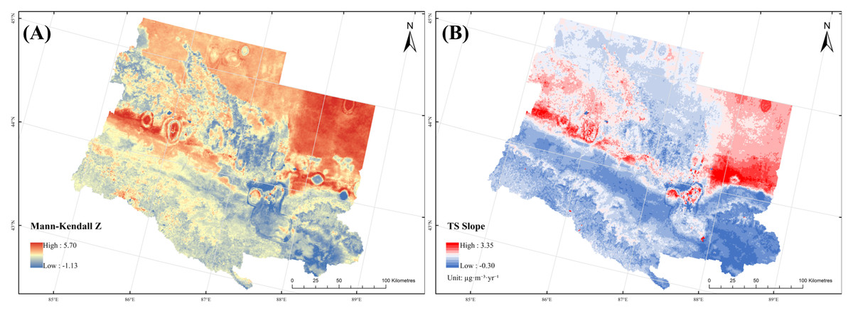
Figure 15: (A) Per-pixel Mann–Kendall Z value and (B) TS slope value of O3 from 2000 to 2022.
(A) Mann–Kendall Z-value map showing the statistical significance of temporal trends in O3 concentrations. Positive Z-values (warm colors) indicate increasing trends, while negative values (cool colors) indicate decreasing trends. |Z|> 1.96 corresponds to a statistically significant trend (p < 0.05). The color gradient ranges from –1.13 to 5.70. (B) Theil–Sen slope map illustrating the magnitude of O3 concentration change over time. Values represent the estimated slope of change in µg m−3 yr−1, with positive values (orange/red) indicating an increase and negative values (blue) a decrease. The slope values range from –0.30 to 3.35 µg m−3 yr−1. Both maps are overlain on a base map of the study region and include a scale bar (0–100 KM) and north arrow for spatial reference.
In regions where MK-Z values indicate significant increases but TS Slope values remain relatively low, the trend represents a gradual yet significant increase. This may be attributed to steady growth in emission source intensity or inhibition of ozone production by topographic factors (e.g., mountainous terrain). Conversely, areas with significant MK-Z decreases but small TS Slope declines exhibit gradual yet significant decreases, potentially due to stable ecological purification capacity or limited effectiveness of mitigation measures. In the central urban agglomeration and adjacent areas, both MK-Z and TS Slope values approach 0, defining a zone of insignificant trends and slow changes. These regions are influenced by stable anthropogenic emissions and unaltered natural factors, leading to a relatively balanced ozone production-depletion dynamic.
Correlation analysis between pollutants and meteorological factors with GRD
Spearman correlation analysis (Fig. 16A) revealed strong and significant negative correlations between PM2.5 and NDVI (ρ = −0.89), T, (ρ = −0.87), PET (ρ = −0.83), and WIND (ρ = −0.77), with P (ρ = −0.71) also moderately negatively correlated. These results suggest that stagnant meteorological conditions—characterized by low PET, low T, weak Winds, and sparse vegetation—are conducive to PM2.5 retention, while higher precipitation enhances wet scavenging. GRA results (Fig. 16B) indicated a different emphasis, ranking P (0.6229) highest, followed by NDVI (0.56846), PET (0.55139), T (0.52758), and WIND (0.52737), underscoring precipitation’s dominant role in wet deposition and vegetation’s importance in pollutant capture. To assess robustness, we repeated Spearman analyses under |ρ| ≥ 0.3 and |ρ|≥ 0.7 thresholds and compared with GRA rankings. The order of dominant drivers (precipitation–vegetation–PET) remained consistent, confirming that our identification of key meteorological factors is stable across analytical approaches and parameter settings.
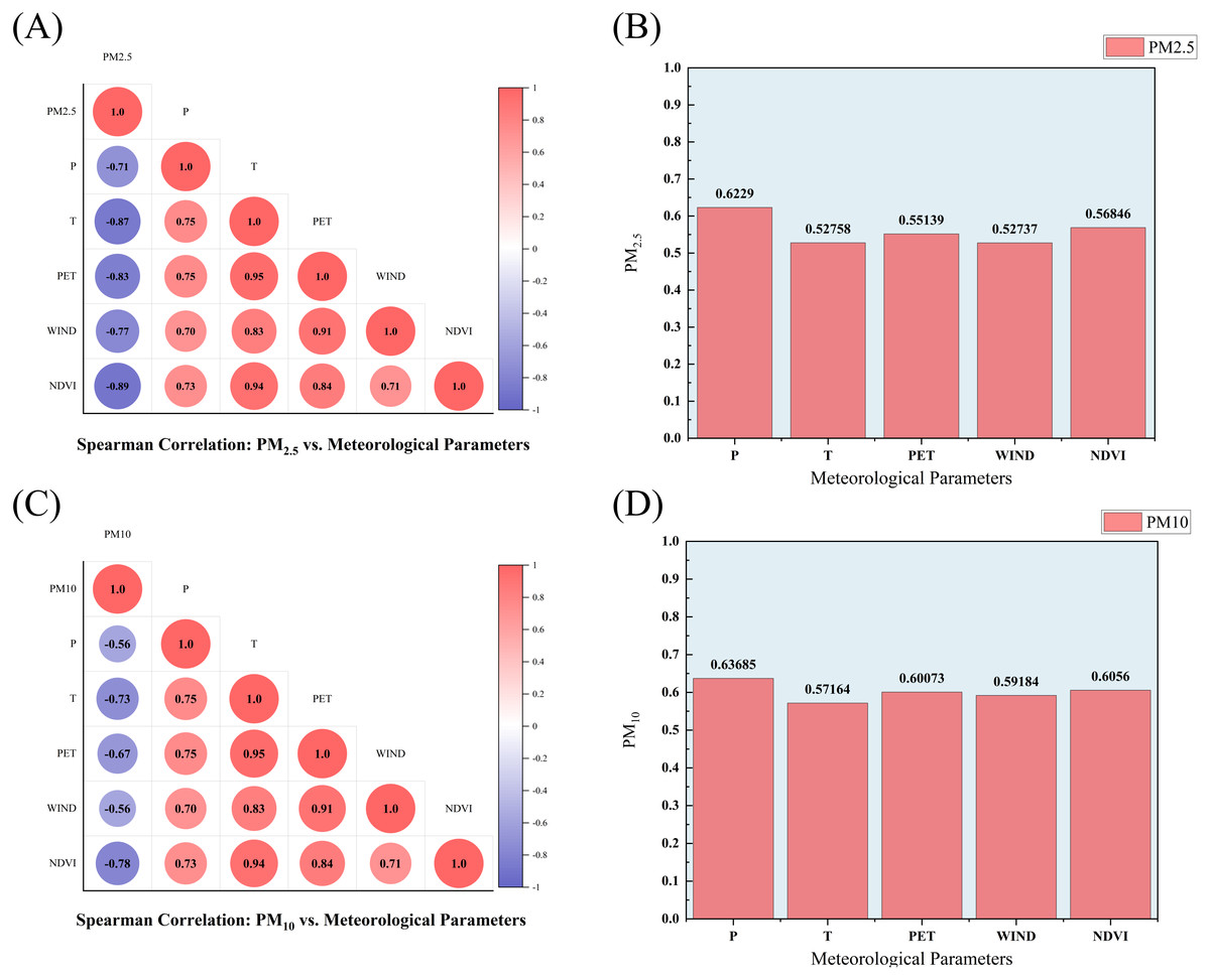
Figure 16: Spearman correlation analysis and grey correlation for PM2.5 and PM10.
(A) Spearman correlation matrix for PM2.5. The matrix depicts the monotonic correlation coefficients between PM2.5 and key meteorological parameters: P, T, PET, WIND, and NDVI. Color intensity (blue to red) and circle size represent the strength and direction of the correlation, ranging from −1 (strong negative, dark blue) to +1 (strong positive, dark red). Numerical values within each circle indicate the exact correlation coefficient. (B) GRA for PM2.5. The red bars (labeled “PM2.5” in the legend) quantify the association strength between PM2.5 and each meteorological parameter, as derived from GRA. Higher values (e.g., 0.6229) indicate a stronger geometric similarity and closer relationship between the data series of PM2.5 and the respective factor over time, irrespective of linearity. (C) Spearman correlation matrix for PM10. This panel follows the same representation as (A) but analyzes the correlations between PM10 and the identical set of meteorological variables (P, T, PET, WIND, NDVI). (D) GRA for PM10. The red bars (labeled “PM10”) display the grey relational degree between PM10 and each meteorological parameter. Similar to (B), this measure assesses the strength of association based on the similarity of development trends and geometric patterns in the data sequences. Collectively, this figure integrates non-parametric statistical (Spearman) and GRA to provide a comprehensive assessment of the relationships between particulate matter concentrations and influential meteorological drivers, highlighting both monotonic dependencies and pattern-based associations.
Spearman correlation analysis (Fig. 16C) showed that PM10 had the strongest negative correlations with NDVI (ρ = −0.78) and T (ρ = −0.73), indicating that higher vegetation coverage and warmer conditions can reduce PM10 levels through interception, adsorption, and enhanced convection. PET (ρ = −0.67) and WIND (ρ = −0.56) also showed negative relationships, suggesting that increased atmospheric motion supports pollutant dispersion, while P (ρ = −0.56) reflected moderate wet scavenging effects. GRA results (Fig. 16D) ranked P (0.63685) highest, followed by NDVI (0.6056), PET (0.60073), WIND (0.59184), and T (0.57164), again emphasizing precipitation’s primary role in PM10 removal. Robustness checks using Spearman thresholds of —ρ— ≥ 0.3 and —ρ— ≥ 0.7 produced rankings consistent with GRA, with P, vegetation, and PET always emerging as the top three drivers. This alignment demonstrates that the meteorological influences on PM10 are stable across different statistical criteria.
Spearman correlation and grey relational analysis (Figs. 17A–17B) together revealed the main meteorological drivers of O3 variation. PET emerged as the most influential factor in both methods (ρ = 0.90; GRD = 0.727), indicating a dual role as a monotonic predictor and a synchronous trend driver, likely reflecting its control over surface energy balance and photochemical reaction rates. WIND ranked second in importance, with a high Spearman coefficient (ρ = 0.83) and substantial GRD (0.681), suggesting a near-linear role in pollutant transport and dispersion. T showed the largest discrepancy between methods—its high Spearman correlation (ρ = 0.88) contrasted with the lowest GRD (0.553)—implying that thermally driven photochemical processes may be subject to non-stationary behavior or temporal variability. P (ρ = 0.66; GRD = 0.695) and NDVI (ρ = 0.76; GRD = 0.615) both exhibited moderate linear correlations but relatively higher grey relational degrees, suggesting that their influence on O3 likely operates through lagged or non-linear pathways. A robustness check—repeating Spearman analysis under correlation thresholds —ρ— ≥ 0.3 and —ρ— ≥ 0.7 and comparing with GRA rankings—confirmed PET and WIND as consistently dominant drivers, with P, NDVI, and T contributing secondary effects. These results highlight the complementary value of combining linear (Spearman) and non-linear (GRA) frameworks to capture both immediate correlations and underlying trend synchrony in detecting O3 driving mechanisms.
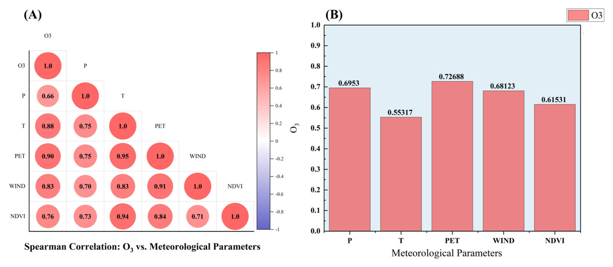
Figure 17: (A) Spearman correlation analysis and (B) grey correlation for O3.
(A) Pearson correlation matrix between O3 and key environmental factors. The matrix displays correlation coefficients for P, T, PET, WIND, and NDVI. Color intensity (blue for negative, red for positive) and circle size represent the strength and direction of the linear correlation, ranging from −1 to +1. Numerical values inside each circle indicate the exact correlation coefficient. (B) Bar chart illustrating the association strength between O3 and each environmental factor. The height of the red bars (labeled “O3” in the legend) and the accompanying numerical values (e.g., 0.6953, 0.72688) quantify the magnitude of the relationship, reflecting the relative influence of each meteorological and vegetation factor on O3 concentration variability. Collectively, this figure integrates parametric statistical correlation analysis (A) and association strength assessment (B) to provide a comprehensive evaluation of the environmental drivers of O3 pollution, highlighting both the directionality and relative power of these influential factors.
Spearman correlation analysis quantifies the statistical correlation between meteorological elements and pollutants, reflecting the strength of linear correlation of variables and the immediate impact of meteorological elements on pollutants. Grey correlation analysis is based on the trend similarity between meteorological elements and pollutant sequences, analyzing the potential mechanism of elemental dynamics on pollutants. Due to the differences in the logic and methodology of statistical correlation and trend similarity, the results of the impact assessment of meteorological factors on pollutants are different in terms of the ranking of the degree of correlation and the characterization of their effects. Furthermore, related studies have also mentioned the differences between the methods (Zheng et al., 2023).
PM2.5 and PM10 (Fig. 18) exhibited a strong positive correlation (ρ = 0.89), reflecting their overlapping anthropogenic emission sources. Coal-fired power plants and motor vehicle exhausts release both fine (PM2.5) and coarse (PM10) particles, and incomplete fossil fuel combustion often produces a bimodal particle size distribution. Meteorological influences on the two pollutants are largely consistent: under stable atmospheric conditions, low WIND, and temperature inversion layers, the diffusion of fine particles and deposition of coarse particles are inhibited, leading to their synchronous accumulation. During rainy periods, both are subject to wet deposition through humidity-driven scavenging.
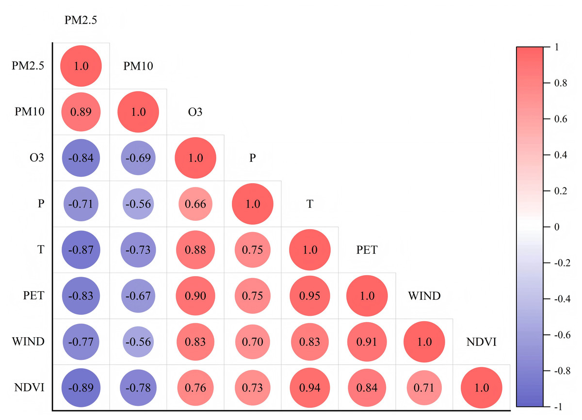
Figure 18: Correlation between pollutants and meteorological elements.
This heatmap visualizes the Pearson correlation coefficients between key atmospheric pollutants (PM2.5, PM10, O3) and meteorological/vegetation parameters. The strength and direction of linear relationships are encoded through a bivariate visual system: color gradient (from dark blue for −1 to dark red for +1) and circle size (proportional to the absolute correlation value). The exact numerical coefficient is displayed within each circle. The color bar on the right provides a continuous scale for interpreting the correlation magnitude and direction. This type of visualization is a standard and powerful method for initial exploratory data analysis, helping to identify potential associations and multicollinearity among variables in environmental studies.
A strong negative correlation was observed between PM2.5 and O3 (ρ = −0.84), indicative of a photochemical competition for common precursors, such as nitrogen oxides (NOx). PM2.5 also exerts a radiative shielding effect by absorbing and scattering ultraviolet radiation, thereby weakening key photolysis reactions essential for O3 formation.
For PM10, mineral aerosols (e.g., dust) can catalyze O3 decomposition (O3 → O2). This effect is especially evident during northern spring dust events, where increases in PM10 concentrations correspond to decreased O3 levels. As coarse particles (2.5–10 µm) are less directly involved in photochemical reactions, the negative PM10–O3 correlation likely reflects indirect associations, such as dust events accompanied by strong WIND, rather than direct atmospheric chemistry.
HYSPLIT forward and backward trajectory analysis
The HYSPLIT_4 developed by the NOAA Air Resources Laboratory was employed to simulate air mass backward and forward trajectories, in order to investigate potential transboundary pollution transport affecting the study area. The model was driven by the Global Data Assimilation System (GDAS) meteorological dataset with a horizontal resolution of 0.25° × 0.25°, a vertical layering of 38 levels, and a temporal resolution of 3 h.
The trajectory simulations were initialized from the central Urumqi site (43.97°N, 87.34°E) at three release heights above ground level (AGL): 500 m (boundary layer), 1,000 m (lower free troposphere), and 3,000 m (high-level transport layer), to account for vertical variability in transport pathways. Both 72-hour backward and forward trajectories were computed at 1-hour time steps to capture synoptic-scale transport events. The emission assumption was set as an instantaneous and homogeneously mixed release of a non-reactive tracer, with no consideration of dry/wet deposition or chemical transformation, as the primary aim was to track air parcel origins and dispersion pathways rather than perform chemical fate modeling.
Model uncertainties may arise from several factors, including (i) errors in meteorological input data, especially in complex terrain; (ii) sensitivity of the calculated trajectories to the choice of starting location, time, and release height; (iii) cumulative divergence of trajectories at extended simulation lengths beyond 72 h; and (iv) model assumptions that exclude atmospheric chemistry, deposition processes, and small-scale turbulence. To assess sensitivity, additional simulations were conducted with varied release heights (±500 m) and durations (48 h vs. 72 h). Results indicate that higher-altitude trajectories are generally more stable, whereas near-surface trajectories in winter are more variable due to valley winds and thermal inversions. These uncertainty sources were considered when interpreting the trajectory results in the discussion section.
As shown in Fig. 19A, regarding back-tracing trajectories, we find that low-level air parcels released at 500 m AGL originated from the northwestern region, starting from eastern Kazakhstan, then approaching the source area over the next few days, about 800 km. At the same time, this air mass descends gradually from 1,500 m to 500 m along the way. This can be attributed mainly to the airflow descending through the northern slope of Tianshan Province due to terrain. As the high-level trajectory moves eastward towards Central Asia, specifically from the northern part of the Caspian Sea within the Volga River Basin, there is almost no movement at high altitudes, with a very small upward speed reaching up to only 0.2 cm/s, indicating stable conditions for upper-level westerlies.
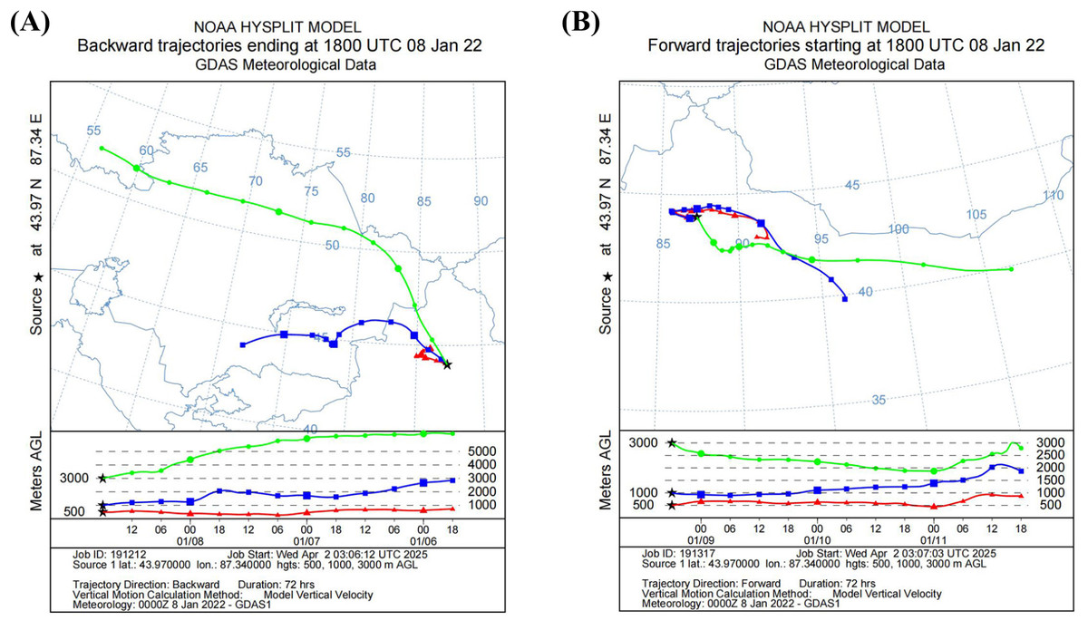
Figure 19: (A) Backward trajectory diagrams and (B) Forward trajectory diagrams.
Air mass trajectories simulated via the NOAA HYSPLIT model with GDAS meteorological data, containing two: (A) backward trajectories terminating at 1800 UTC on 08 January 2022. (B) Forward trajectories initiating at 1800 UTC on 08 January 2022. In both subplots, colored lines denote trajectories at distinct heights above ground level (AGL): red corresponds to 500 m AGL, blue to 1,000 m AGL, and green to 3,000 m AGL. The lower panels in each subplot depict the vertical change of trajectory height over time, while the maps illustrate horizontal trajectory paths. The model simulates trajectory dynamics over a 72-hour period.
Further analysis shows that the large-scale circulation is affected by strong west winds, which contribute significantly to the high-level advection transfer caused by the Siberian High Pressure system (a high pressure center greater than 1,040 hPa), forcing low-level northerly cold air southwards. On one hand, mesoscale topography has an important impact because of the obstruction of mountains around Tien Shan Mountain Range or forcing the mountain uplift phenomenon. On the other hand, lake Balkhash’s heat contrast also affects the direction of low-level flow. Additionally, boundary layer diffusion such as nocturnal inversion processes inhibits the vertical diffusion of low-level air currents, causing them to stagnate near the transport layer.
As shown in Fig. 19B, the low-level trajectory shows southeast movement and forms a zigzag line about 600 km, mainly affected by the friction of the northern foothills of Tianshan Mountains and local circulation; the middle-layer acceleration to the east and reaching the western part of Mongolian Plateau is due to high-level momentum downward transmission; intermediate-level accelerated eastward to the western region of the Mongolian Plateau, indicating that high level also contributed to the momentum transportation. In general, the high-level trajectory is mainly controlled by strong westerlies, and its track is relatively straight, transporting the longest distance and finally arriving at North China. Trajectory scattering is caused by the influence of westerly jet stream, the effect of pressure gradient on Mongolia, and the influence of the topography of Tianshan Mountain; the curved low-level route may be related to the temperature, barometer in Dzungarian Basin, and mountain leeward wave dynamic conditions.
These simulations can provide us with more information to better understand transboundary pollutants transported from Central Asia during winter, especially for the pollution transport in central Eurasia region. The result has demonstrated the prominent westerly transport channel at an altitude of 3,000 m, which could provide some basic evidence to study long-range high-level sand-dust aerosol transport in further works.
Discussion
This study shows that PM2.5 and PM10 in the U-Chang-Shi urban agglomeration display a clear spatial convergence. Seasonal variations of both pollutants are closely aligned. Rapid economic growth, industrial development, and urban construction are the main emission sources (Zhou, Zhao & Yang, 2017). A PM10 hotspot was identified in the southeast of Urumqi, near Turpan. This is due to valley terrain and airflow patterns that slow dispersion and cause accumulation.
Urumqi’s terrain is a major factor in pollution retention. The city is surrounded by mountains on three sides and opens only to the southeast, forming a “trumpet-shaped” basin. This limits ventilation and favors stagnation. In winter, radiative cooling strengthens inversion layers and suppresses vertical mixing. Frequent southeasterly “burning winds” transport pollutants into the basin and interact with northward valley winds. This causes convergence of pollutants from several directions (Li et al., 2022). In 2023, the U-Chang-Shi joint prevention and control programme reduced PM2.5 by 34%, but PM10 fell only 12% (Chen et al., 2024). Coarse particles remain a challenge, especially under burning-wind conditions. Future policies should focus on dust control in upwind areas, vegetation and windbreak barriers, and improved transboundary monitoring.
Our findings in the U-Chang-Shi share similar patterns with other arid and semi arid regions of Asia. In Central Asia, including Kazakhstan and Uzbekistan, strong seasonal PM peaks are closely linked to dust storms and limited atmospheric mixing. Westerly transport channels at altitudes around 3,000 m carry dust over long distances in winter (Chu et al., 2021; De Beurs & Henebry, 2004), similar to burning wind driven transport in the U-Chang-Shi area. These regions also experience pollutant retention due to basin-like terrain and winter inversions. In Pakistan’s arid areas, PM concentrations peak before the monsoon due to intense dust activity and low rainfall, while O3 peaks in warm seasons under strong sunlight (Deng et al., 2021). This mirrors our observation of seasonal PM–O3 decoupling, driven by photochemical reactions. On the Loess Plateau in north central China, PM trends are strongly influenced by land use changes and regional meteorology (Peng et al., 2017a; Peng et al., 2017b; Ding & Peng, 2020). Compared with U-Chang-Shi, dust peaks there are more coupled with anthropogenic emissions in spring, while in “U-Chang-Shi”, PM10 peaks are dominated by burning wind transport from deserts. These comparisons indicate that integrated PM–O3 control is a common challenge across arid Asia. Dust source stabilization, regional atmospheric forecasting, and joint transboundary emission inventories, as practiced in parts of Central Asia, could inform management strategies for U-Chang-Shi and similar regions in China.
Although the CHAP satellite dataset performs well in arid regions (R2 > 0.67), limitations exist. Persistent cloud cover or seasonal snow can reduce retrieval accuracy and introduce seasonal bias. The HYSPLIT model also has constraints. It depends on meteorological input quality and resolution. Here, GDAS data at 0.25° resolution were used. This is sufficient for large-scale patterns but cannot fully capture local circulations or sub-grid turbulence. Valley winds and mesoscale eddies may be underrepresented, creating uncertainty in transport pathways. Future work should use higher resolution meteorological data, better retrieval algorithms, and integrated chemical–transport models.
O3 pollution patterns differ from those of particulate matter. High O3 levels occur in spring and summer, especially near the Urumqi Chemical Industry Park. Photochemical reactions driven by industrial VOC emissions and favorable meteorological conditions are key contributors. Since 2017, O3 levels have increased by 4.6% per year, coinciding with coal-to-chemical industry expansion. This indicates that control strategies focusing only on PM can unintentionally raise O3. Coordinated VOC and NOx reduction is essential. Effective actions include stricter emission standards, adoption of low-reactivity solvents, and catalytic control technologies.
Changes in air quality in the U-Chang-Shi area have significant socio-economic impacts. The “coal-to-gas” programmed lowered PM2.5 and supported clean energy growth. However, rising O3 may increase respiratory illness, strain healthcare systems, and reduce productivity. Air quality policies should integrate pollution control with industrial transformation and public health planning.
Nonetheless, it is imperative to acknowledge that the integration of socio-economic covariates is crucial for effectively disentangling anthropogenic policy effects from meteorological variability. Previous studies have successfully linked emission trends with economic growth and variations in industrial structure (Zhao et al., 2020; Zhou, Zhao & Yang, 2017). As a future research direction, we plan to develop a generalized additive model (GAM) framework that incorporates prefecture-level coal consumption, GDP, and industrial emission inventory data alongside key meteorological variables. This integration aims to enhance our understanding of the drivers of air quality change in the U-Chang-Shi region, enabling more nuanced and effective policy formulations.
Three future priorities emerge from this study. First, strengthen cross-regional cooperation and targeted action for burning-wind events. Second, apply joint PM2.5–O3 control with balanced reduction goals. Third, integrate weather forecasts and topography into seasonal and event-based emergency policies.
By linking meteorology, pollutant transport, comparative regional analysis, and socio-economic effects, this study offers evidence to improve air quality strategies in arid-region urban clusters, and the findings may guide similar areas balancing economic growth and environmental protection.
Conclusions
This study analyzed the spatial and temporal variations of PM2.5, PM10, and O3 in the U-Chang-Shi urban agglomeration in northwest China from 2000 to 2022, using the CHAP dataset. The results show that CHAP data are highly consistent with observations from state-controlled stations, confirming its suitability for long-term aerosol monitoring in arid urban clusters.
Pollutant accumulation in U-Chang-Shi is influenced by a combination of factors. The trumpet-shaped basin topography and frequent winter inversions limit vertical dispersion. Southeast burning winds transport coarse particles over long distances, adding to local emissions from rapid urbanization, coal combustion, and the chemical industry. These factors increase aerosol residence time and promote complex pollution events. The coal-to-gas project (2012–2015) reduced PM2.5 concentrations by 34%, but PM10 decreased by only 12% due to dust transport limitations. Since 2017, O3 levels have risen at 4.6% per year, indicating the limits of traditional particle-focused control measures in achieving multi-pollutant reduction.
Compared with other Asian arid cities, U-Chang-Shi shares several features. In Central Asian basins, winter PM peaks and pollutant retention are common, but dust events in U-Chang-Shi are more strongly driven by burning winds (Li et al., 2022; Chen et al., 2022). O3 patterns are similar to those in arid Pakistan, where summer peaks are linked to photochemical reactions under high radiation (Noreen et al., 2018; Yang et al., 2025). On China’s Loess Plateau, springtime dust is more related to agricultural activity, while U-Chang-Shi dust is dominated by windborne transport from desert regions (Kang et al., 2024). These comparisons show that compound pollution and PM–O3 co-control are shared challenges across arid Asia (Wei et al., 2020; Duan et al., 2023).
This study is novel in combining high-resolution CHAP satellite data with long-term multi-pollutant analysis to reveal transport processes in an arid urban cluster. It confirms the monitoring value of CHAP for such regions and identifies the key role of burning-wind-driven PM10 transport. However, seasonal differences in meteorological drivers were not fully quantified, and the role of land-use change on O3 formation remains unclear.
Based on our findings, several actions are recommended. First, implement dust control in upwind desert areas, establish vegetation barriers, and strengthen suppression measures during burning-wind seasons. Second, adjust NOx/VOC reduction ratios, build a VOC fingerprint database, and map dynamic O3 production potential for targeted regulation. Third, develop a cross-regional joint control platform integrating monitoring, forecasting, and source tracing, learning from regional forecasting systems in Central Asia. Finally, combine high-resolution land-use and weather data to design season-specific pollution control strategies.
Supplemental Information
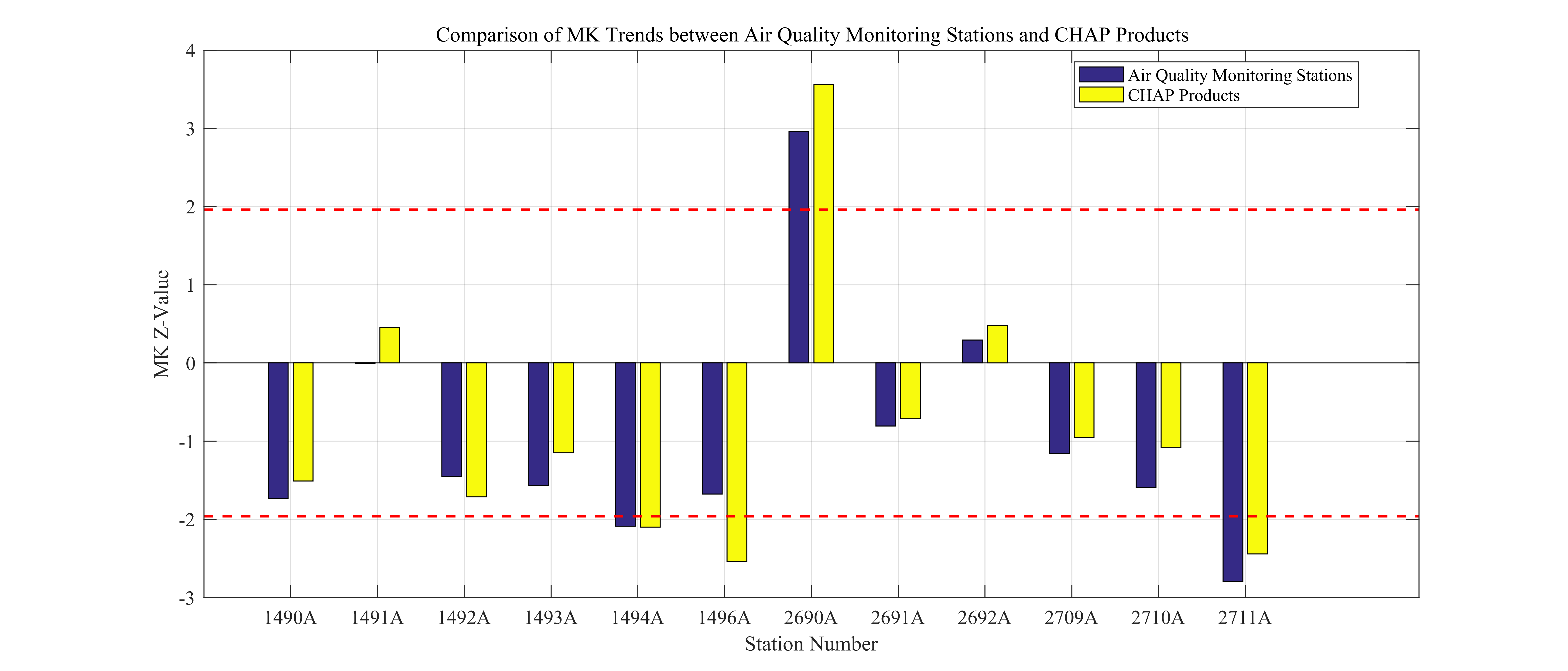
Comparison of MK trends between air qualiy monitoring stations and CHAP products
This bar chart compares Mann–Kendall (MK) trend Z-values between two data sources across multiple stations: dark blue bars: Z-values derived from air quality monitoring stations.Yellow bars: Z-values derived from CHAP products. Red dashed lines: critical values of Z = ± 2 (marking the threshold for statistical significance at the 0.05 level in MK trend tests). The x-axis denotes station numbers, while the y-axis represents MK Z-values (positive values indicate increasing trends, negative values indicate decreasing trends, and magnitude reflects significance relative to the critical values).