
Unraveling habitat-driven shifts in alpha, beta, and gamma diversity of hummingbirds and their floral resource
- Published
- Accepted
- Received
- Academic Editor
- Sandrine Pavoine
- Subject Areas
- Biodiversity, Conservation Biology, Ecology
- Keywords
- Alpha diversity, Beta diversity, Floral resources, Habitat-driven diversity, Hummingbirds, Gamma diversity
- Copyright
- © 2024 Martínez-Roldán et al.
- Licence
- This is an open access article distributed under the terms of the Creative Commons Attribution License, which permits using, remixing, and building upon the work non-commercially, as long as it is properly attributed. For attribution, the original author(s), title, publication source (PeerJ) and either DOI or URL of the article must be cited.
- Cite this article
- 2024. Unraveling habitat-driven shifts in alpha, beta, and gamma diversity of hummingbirds and their floral resource. PeerJ 12:e17713 https://doi.org/10.7717/peerj.17713
Abstract
Background
Biodiversity, crucial for understanding ecosystems, encompasses species richness, composition, and distribution. Ecological and environmental factors, such as habitat type, resource availability, and climate conditions, play pivotal roles in shaping species diversity within and among communities, categorized into alpha (within habitat), beta (between habitats), and gamma (total regional) diversity. Hummingbird communities are influenced by habitat, elevation, and seasonality, making them an ideal system for studying these diversities, shedding light on mutualistic community dynamics and conservation strategies.
Methods
Over a year-long period, monthly surveys were conducted to record hummingbird species and their visited flowering plants across four habitat types (oak forest, juniper forest, pine forest, and xerophytic shrubland) in Tlaxcala, Mexico. Three locations per habitat type were selected based on conservation status and distance from urban areas. True diversity measures were used to assess alpha, beta, and gamma diversity of hummingbirds and their floral resources. Environmental factors such as altitude and bioclimatic variables were explored for their influence on beta diversity.
Results
For flowering plants, gamma diversity encompassed 34 species, with oak forests exhibiting the highest richness, while xerophytic shrublands had the highest alpha diversity. In contrast, for hummingbirds, 11 species comprised the gamma diversity, with xerophytic shrublands having the highest richness and alpha diversity. Our data reveal high heterogeneity in species abundance among habitats. Notably, certain floral resources like Loeselia mexicana and Bouvardia ternifolia emerge as key species in multiple habitats, while hummingbirds such as Basilinna leucotis, Selasphorus platycercus, and Calothorax lucifer exhibit varying levels of abundance and habitat preferences. Beta diversity analyses unveil habitat-specific patterns, with species turnover predominantly driving dissimilarity in composition. Moreover, our study explores the relationships between these diversity components and environmental factors such as altitude and climate variables. Climate variables, in particular, emerge as significant contributors to dissimilarity in floral resource and hummingbird communities, highlighting the influence of environmental conditions on species distribution.
Conclusions
Our results shed light on the complex dynamics of hummingbird-flower mutualistic communities within diverse habitats and underscore the importance of understanding how habitat-driven shifts impact alpha, beta, and gamma diversity. Such insights are crucial for conservation strategies aimed at preserving the delicate ecological relationships that underpin biodiversity in these communities.
Introduction
The study of biodiversity, the variety of life forms within ecosystems, help us understand the organization, complexity, interconnectedness and resilience of communities (Tilman, Reich & Knops, 2006; Campbell, Murphy & Romanuk, 2011). Its study extends beyond a mere cataloging of species; it involves a comprehensive examination of the richness, composition, and distribution of species, spanning from local to regional scales (Jost, 2006). Ecological factors, both biotic (i.e., species interactions) and abiotic (e.g., temperature and precipitation), influence the distribution of species and population density within a community (Pearson & Dawson, 2003; Benton, 2009). These environmental and biological factors act as filters that determine which species can survive and thrive in a specific area, and their coexistence is contingent upon their specific needs and requirements based on competition for resources (Wisz et al., 2013). This way, diversity within communities is primarily shaped by these ecological processes (Chesson, 2000).
It is widely recognized that species diversity exhibits spatial heterogeneity. For example, at a regional scale, significant disparities in species richness have been widely documented among habitats (e.g., MacArthur, 1965; Būhning-Gaese, 1997). These spatial trends have given rise to the concept of three levels of species diversity: alpha (α), beta (β), and gamma diversity (γ) (Whittaker, 1960). The partitioning of biodiversity into three components offers a powerful framework to unravel the intricacies of these diversity patterns. Firstly, alpha diversity characterizes species richness and abundance within a single habitat, providing insights into the structure of local communities. Secondly, beta diversity quantifies the turnover of species between habitats, shedding light on the ecological processes driving community assembly and turnover. Lastly, gamma diversity, encompassing total species richness across multiple habitats, reflects broader regional diversity patterns (Whittaker, 1960). Fundamental topics in ecological research have revolved around distribution patterns and mechanisms that maintain species diversity across environmental gradients (Lyons & Willig, 2002; McCain, 2009; Wang et al., 2007). Understanding these patterns and mechanisms is crucial for devising strategies and measures aimed at preserving species diversity in the face of environmental changes.
Because of their feeding ecology, hummingbirds (Aves: Trochilidae) are closely tied to their floral resources (Abrahamczyk & Kessler, 2015). Their extreme specialization in dependence on nectar consumption has led these tiny birds to often track the availability of nectar sources by following the blooming of flowers, an ability that enables them to survive and thrive in various habitats across the Americas (Leimberger et al., 2022). The dynamics shaping hummingbird communities have been explored in numerous studies, revealing an intriguing trend. Hummingbird communities in low-lying habitats (≤50 m a. s. l.), encompassing both dry and humid forests, experience an upsurge in both species richness and abundance (Buzato, Sazima & Sazima, 2000). In contrast, a different scenario unfolds in habitats surrounded by temperate vegetation at higher and colder elevations (>2,000 m a. s. l. with temperatures around −5 °C), such as cloud forests and coniferous forests. In these habitats, there is a tendency for a decrease in the richness and abundance of hummingbird species (Graham et al., 2009; Partida-Lara et al., 2018). Interestingly, this general pattern doesn’t account for the remarkable species richness in the montane region of the Andes, where elevation has instead generated diverse topographical features that have promoted high speciation rates (Rahbek et al., 2007).
In addition to the habitat type’s impact on the structure of hummingbird communities, seasonality also exerts an effect due to variations in environmental variables that directly influence the floral resources they utilize, such as precipitation. In this regard, it has been demonstrated that in habitats with scarce precipitation, such as tropical dry forests, the peak flowering of plants visited by hummingbirds primarily occurs during the dry season (Arizmendi & Ornelas, 1990; Bustamante-Castillo, Hernández-Baños & Arizmendi, 2018; Martínez-García, González & Ortiz-Pulido, 2020). Conversely, in temperate environments such as conifeous forests, the flowering peaks of these plants align with the rainy season (Des Granges, 1979; Lara, 2006). In response to this seasonal effect in the environment, there is typically a positive relationship where a greater number of flowers (i.e., flowering peaks) denotes higher diversity and abundance of hummingbirds at the local level (Cotton, 2007). Therefore, the dynamics of this relationship over time can led hummingbird communities to undergo restructuring (Wolf, Stiles & Hainsworth, 1976; Arizmendi & Ornelas, 1990; Lara, 2006).
The interaction between hummingbirds and flowers is an ideal context to explore the three diversity components. The diversity of both these groups may be influenced by factors such as resource availability, and habitat specialization. By dissecting the alpha, beta, and gamma diversity patterns within this context, we aim to uncover the mechanisms driving the assembly and maintenance of these intricate mutualistic communities. Central Mexico is a hotspot of ecological diversity, characterized by its varied topography, altitude gradients, and climatic variability (Sánchez-Cordero et al., 2005). This ecological heterogeneity provides a unique backdrop for exploring biodiversity patterns and underlying ecological processes. Among the states within this region, Tlaxcala, the smallest state in the country (after the capital Mexico City), holds a unique geographical position that facilitated the collection of comprehensive data on the diversity of hummingbirds and their flowers across different vegetation types. This provided insights into the dynamics of these communities within a confined yet ecologically diverse area.
The main goal of our research was to describe the alpha, beta, and gamma diversity patterns within hummingbird-flower communities across the most representative habitats of the region: the oak forest, pine forest, juniper forest, and xerophytic shrubland. These habitats encompass environmental conditions ranging from typically humid and cold to dry and warm and are mainly found covering altitudinal ranges from 2,400 to 2,700 m a.s.l., although pine forests can be found at elevations as high as 4,000 m a.s.l. at the highest point in the region, La Malinche volcano. Considering the variability in our studied habitats, we expected significant variations in alpha, beta, and gamma diversity in hummingbird-flower communities across oak forest, pine forest, juniper forest, and xerophytic shrubland habitats due to their distinct environmental conditions. Additionally, we hypothesized that abiotic factors such as altitude, temperature, and precipitation would influence species composition between these habitats (beta diversity). Finally, we expected higher alpha diversity in habitats with more varied conditions, while beta diversity will likely correlate with specific environmental factors distinguishing each habitat.
Materials and Methods
Study area
From February 2014 to January 2015, samplings were carried out in four types of vegetation (hereafter referred to as “habitats”) characteristic of the state of Tlaxcala, Mexico: oak forest, juniper forest, pine forest, and xerophytic shrubland. Based on digital land use and vegetation maps at a 1:250,000 scale, as well as information about the vegetation within the state of Tlaxcala (National Institute of Statistics and Geography of Mexico (INEGI), 2009, 2010; Acosta, Delgado & Cervantes, 1992; Luna, Morrone & Espinosa, 2007), three locations were selected for each habitat (Fig. 1). For their selection, these locations met the following requirements: (i) belong to conserved areas according to National Institute of Statistics and Geography of Mexico (INEGI) (2010), (ii) be distant from urban areas (~3 km), and (iii) be separated from each other to ensure sampling independence (average distance between locations greater than 13 km). Subsequently, across three locations, for each of four habitat types, we established five 500 m transects per habitat with 20 m wide bands on each side, with transect number varying between two and one per locality, totaling five transects per habitat type. Maintaining 100 m distance between transects within localities, this design yielded 20 total transects with georeferenced coordinates and altitudes (m a.s.l.) recorded via GPS (Garmin Etrex 30).
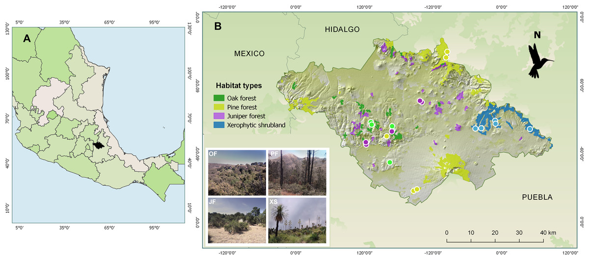
Figure 1: Maps showing (A) the location of the state of Tlaxcala, Mexico (shown in black), and (B) the locations of the monitored habitats, where the diversity of hummingbirds and their flowering plants was studied.
The colored circles represent the transects established for each habitat type: Oak forest (OF) in green, pine forest (PF) in yellow, juniper forest (JF) in purple, and xerophytic shrubland (XS) in blue. Sources: ESRI, Garmin, National Institute of Statistics and Geography of Mexico (INEGI) (2009). Uso del suelo y vegetación, escala 1:250,000, serie IV. 2009, and Qgis version 2.18, 2016. QGIS Geographic Information System. QGIS Association: http://www.qgis.org. Photo credit: Hellen Martínez-Roldán.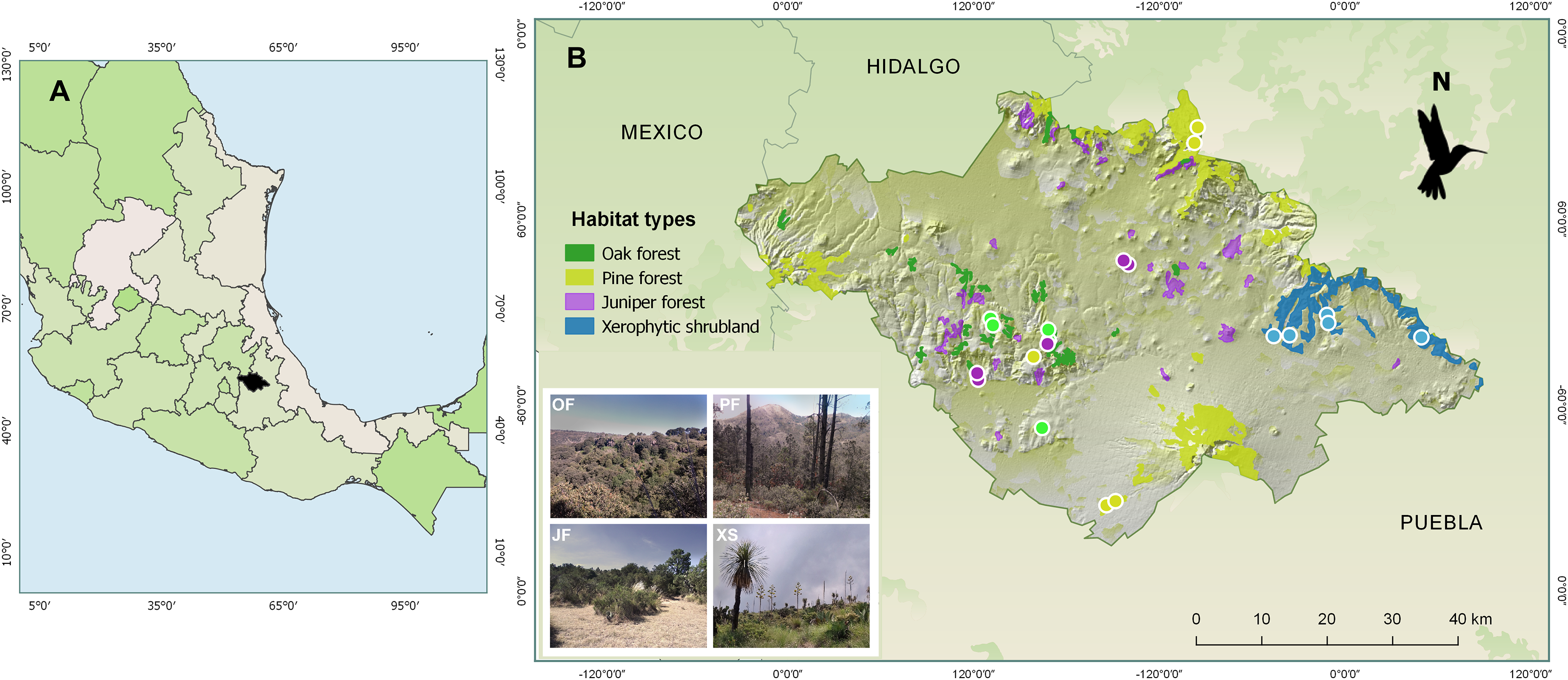
In each location, the transects were established in sites that could encompass the dominant tree species for the habitat type. In oak forest, species of the Quercus genus predominate, such as Q. crassipes, Q. glaucoides, Q. laurina, and Q. mexicana. The dominant tree species in juniper forest is Juniperus deppeana. In pine forest, characteristic species include Pinus montezumae, P. hartwegii, P. patula, and P. leiophylla. Finally, in xerophytic shrubland, dominant species include Yucca filifera, Nolina longifolia, Dasylirion acrotriche, and Opuntia robusta (Fig. 1).
Sampling of hummingbirds and their flower plants
To identify and quantify the abundance of hummingbirds and the flowering plants they visited, monthly surveys were conducted over a 12-month period at five transects established for each habitat type. Sampling was carried out from 8:00 to 13:00 h. During this period, all the hummingbirds detected within the transect were recorded, whether they were observed foraging on the flowers, perched, or in flight. The observed individuals were identified with the assistance of specialized field guides (Williamson, 2001; Arizmendi & Berlanga, 2014). Using this information, we obtained the number of individuals per hummingbird species for each survey.
Concurrently, all plant species within a transect (i.e., plants exhibiting tubular flowers, bright colors, and nectar production; Faegri & van Der Pijl, 1979) were recorded. Species that did not fit the proposed ornithophilous syndrome were also included in the records if hummingbirds were observed foraging on them. Floral abundance was measured as the number of open flowers per plant species in each transect. The identification of plant species was conducted using dichotomous keys (Calderón & Rzedowski, 2001). Sample completeness (sample coverage) for hummingbirds and plant species across habitat types was performed using the ‘iNext’ function from the iNEXT package (Hsieh, Ma & Chao, 2016) in RStudio, ver. 2023.03.0 + 386 (RStudio Team, 2022). The iNEXT package uses a unified framework based on Hill numbers to estimate sample completeness at different sample sizes, incorporating both interpolation (rarefaction) and extrapolation techniques (Chao et al., 2014; Hsieh, Ma & Chao, 2016). By utilizing the ‘iNext’ function, rarefaction is inherently performed as part of the interpolation process, ensuring that sample completeness can be compared across samples with different sizes or sampling efforts.
Diversity measures
Studies focusing on avian diversity often use gamma diversity to assess regional species richness (e.g., Metcalf et al., 2022), alpha diversity for local species composition (e.g., Jarrett et al., 2021), and beta diversity to analyze habitat-based variation (e.g., de Deus et al., 2020). In plant ecology, similar diversity measures elucidate species turnover and richness across various plant communities (e.g., Fontana et al., 2020; Vetaas, Shrestha & Sharma, 2021). Here, to assess the structure and differences in hummingbird and plant assemblages within the study region, we performed an analysis of regional diversity (gamma diversity) by considering all habitats as a unit. Additionally, we conducted a detailed analysis of local diversity within each habitat (alfa diversity), examined how the respective assemblages differ between communities (beta diversity), and explored the origins of differences among habitats, including species turnover and variations in species richness. Furthermore, we assessed the potential role of environmental factors in explaining differences between communities within each habitat. These concepts are pivotal for understanding biological processes across diverse habitats, the structure of biological communities, and the distribution of species at local and regional level. Their practical applications extend to environmental management and conservation of biodiversity.
Each diversity index, H, can be expressed as its true diversity index or equivalent numbers (qD(H)), also referred to as Hill numbers (Jost, 2006; Moreno et al., 2017). Equivalent numbers represent the essential components (i.e., species, communities) that a balanced community with equally common species would possess, assuming that the diversity index of the balanced community matches that of the real community (Jost, 2006, 2010; Pereyra & Moreno, 2013). Thus, effective numbers depict the structure of the real community in equivalent units, enabling comparisons of the degree of change between communities (Jost, 2006, 2007). Effective numbers qD derived from the following formula (Jost, 2007):
where pi is the relative frequency of species i, q is the order of diversity measurement, and S is the number of species. The parameter q has an exponential property that determines the sensitivity of the index to the relative abundance of species (Jost, 2006, 2007). Species richness corresponds to the diversity index of order 0 and is insensitive to the relative frequency of species. The diversity measure of order 1 is equivalent to the exponential of Shannon’s entropy and weights rare and common species proportionally to their abundance. The diversity measures of order 2 are equivalent to Simpson’s inverse measures, which favor abundant species while excluding rare ones (Hill, 1973; Jost, 2006, 2007).
To measure diversity across the region encompassing the four habitat types, we computed the gamma diversity index (qDγ) using the multiplicative partitioning of regional diversity as proposed by Whittaker (1960), where qDγ =qDα*qDβ. The equivalent numbers, expressed as 0Dα, denotes the number of species in the communities (0Dβ) required to match the total species count in the region (0Dγ).
To evaluate diversity at a local level, we calculated alpha diversity (orders q = 0,1,2) for the community composition within each habitat concerning the hummingbird and plant species assemblages.
Among communities, changes in species composition are explained by β diversity (Whittaker, 1960). The β diversity can arise from two processes: species turnover and nestedness; both components identify the source of disparities between communities (Carvalho, Cardoso & Gomes, 2012). These two components explain β diversity additively (βcc = β-turnover + β-nestedness). To derive β diversity and its components (β-turnover, β-nestedness), three measures were calculated: a) species common to both sites, b) species exclusive to one site, and c) species exclusive to the other site (see formulas in Carvalho, Cardoso & Gomes, 2012). βcc represents a proportion of dissimilarity between two communities, where 0 indicates that communities share all species, and one corresponds to communities that do not share any species; however, βcc does not take species abundances into account, while Hill numbers do consider abundance in addition to species richness. Additionally, species turnover (β-turnover) varies from 0 (when species composition is identical) to 1 (when species composition is entirely different). The values of β-nestedness follow the same scale from 0 to 1 (when species richness is equal or different respectively).
Furthermore, following Jost (2007), gamma diversity was calculated for orders q = 0 and q = 1, considering the unequal weighting of plant and hummingbird communities. Alpha diversity, essential for understanding each community’s composition was assessed for orders 0, 1 and 2. Finally, beta diversity and its components across the four habitats for both communities were computed according to Carvalho, Cardoso & Gomes (2012) and Carvalho et al. (2013). All analysis were performed with RStudio, ver. 2023.03.0 + 386 (RStudio Team, 2022), using the vegan package (Oksanen et al., 2022).
The relationship between beta diversity and environmental factors
Subsequently, the correlation of β diversity (βcc, β-turnover, β-nestedness) and environmental factors such as altitude, and 19 bioclimatic variables obtained from the WorldClim website (http://www.worldclim.org), was assessed using Mantel tests (Sokal & Rohlf, 1995). Simple Mantel tests assess the correlation between two dissimilarity matrices, while partial Mantel tests allow controlling for the effect of a third matrix (in this case, the dissimilarity matrix of the other environmental variables) when evaluating the correlation between the two main matrices. These tests enable us to determine if the variation in β diversity among communities is related to differences in the selected environmental variables, which can help understand the factors influencing the structure and composition of communities in the studied region. For this purpose, the values of each bioclimatic variable were extracted for each transect, and a principal component analysis (PCA) was performed to condense the abiotic variables. Highly correlated variables were removed, as well as those with less contribution to the components explaining >90% of the variance. The selected variables were annual precipitation (Bio12), precipitation of wettest quarter (Bio16), and altitude. Dissimilarity matrices were constructed using the Bray-Curtis method for the selected variables. Simple and partial Mantel tests were conducted with 9,999 permutations. The Mantel tests were computed with RStudio, ver. 2023.03.0 + 386 (RStudio Team, 2022), using the vegan package.
Results
Abundance of flowering plants and hummingbirds
The observed number of plant and hummingbird species in the study seemed to reach an asymptote in relation to our sampling effort across the four sampled habitats (a total of 180 h of evenly distributed observation efforts for each habitat throughout the study). For plant species, we detected 99.91% for the oak forest, 99.62% for pine forest, 99.57% for juniper forest and, 99.95% for xerophytic shrubland according to the Chao2 estimator, after conducting 12 samples for each habitat type throughout the study (File S1, Fig. 1S). Likewise, we detected 98.15% of the hummingbird species estimated for the oak forest, 96.25% for pine forest, 98.40% for juniper forest and 95.16% of those estimated for the xerophytic shrubland (File S1, Fig. 2S).
The samplings conducted throughout the study in the four habitat types allowed for the total recording of 34 plant species, which were classified into 22 genera, 17 families, and 11 orders (File S2). Of the total quantified flower abundance, 83% was recorded in five plant species: Loeselia mexicana (24%), Bouvardia ternifolia (14%), Castilleja tenuiflora (18%), Penstemon roseus (16%), and Salvia elegans (11%). The last three plant species belong to the order Lamiales (45% of the total abundance). Likewise, L. mexicana, C. tenuiflora, and B. ternifolia were shared species in all four habitat types, thus being characteristic plant species within the region (Fig. 2A). Therefore, the description of the results hereafter will be particularly based on these plant species, as well as in the case of the hummingbird species referred to below.
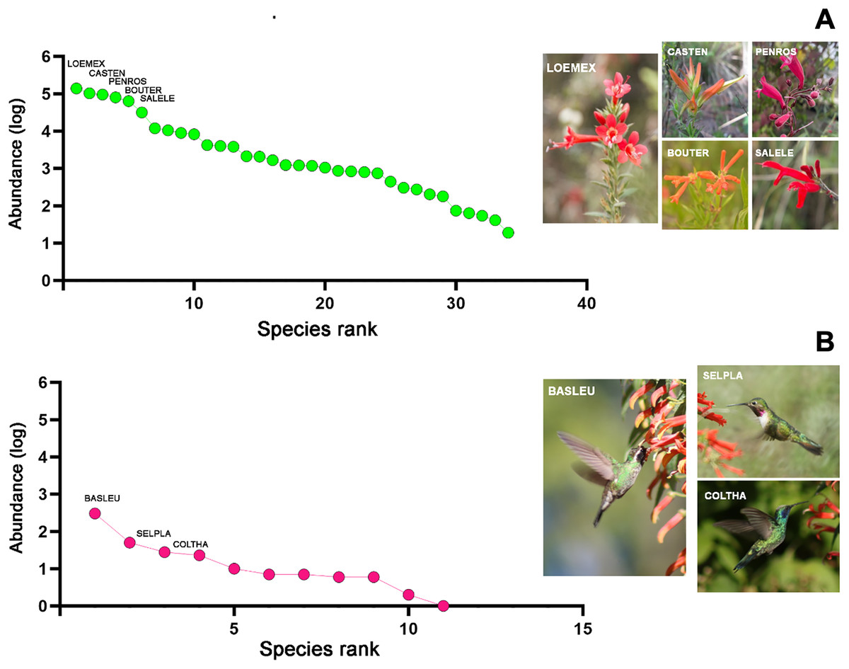
Figure 2: Rank/abundance plots for hummingbirds and their flowering plants species at the regional level in Tlaxcala, Mexico.
Rank/abundance curves show the distribution of plant and hummingbird species from most to least abundant. (A) Loeselia mexicana (LOEMEX), Castilleja tenuiflora (CASTEN), Penstemon roseus (PENROS), Bouvardia ternifolia (BOUTER), and Salvia elegans (SALELE) were the most abundant plant species within the region, while (B) Basilinna leucotis (BASLEU), Selasphorus platycercus (SELPLA), and Colibri thalassinus (COLTHA) highly dominate in all sampled habitat types. Photo credit: Ubaldo Marquez-Luna, Hellen Martínez-Roldán, Juan Manuel González, María José Pérez-Crespo and Carlos Lara.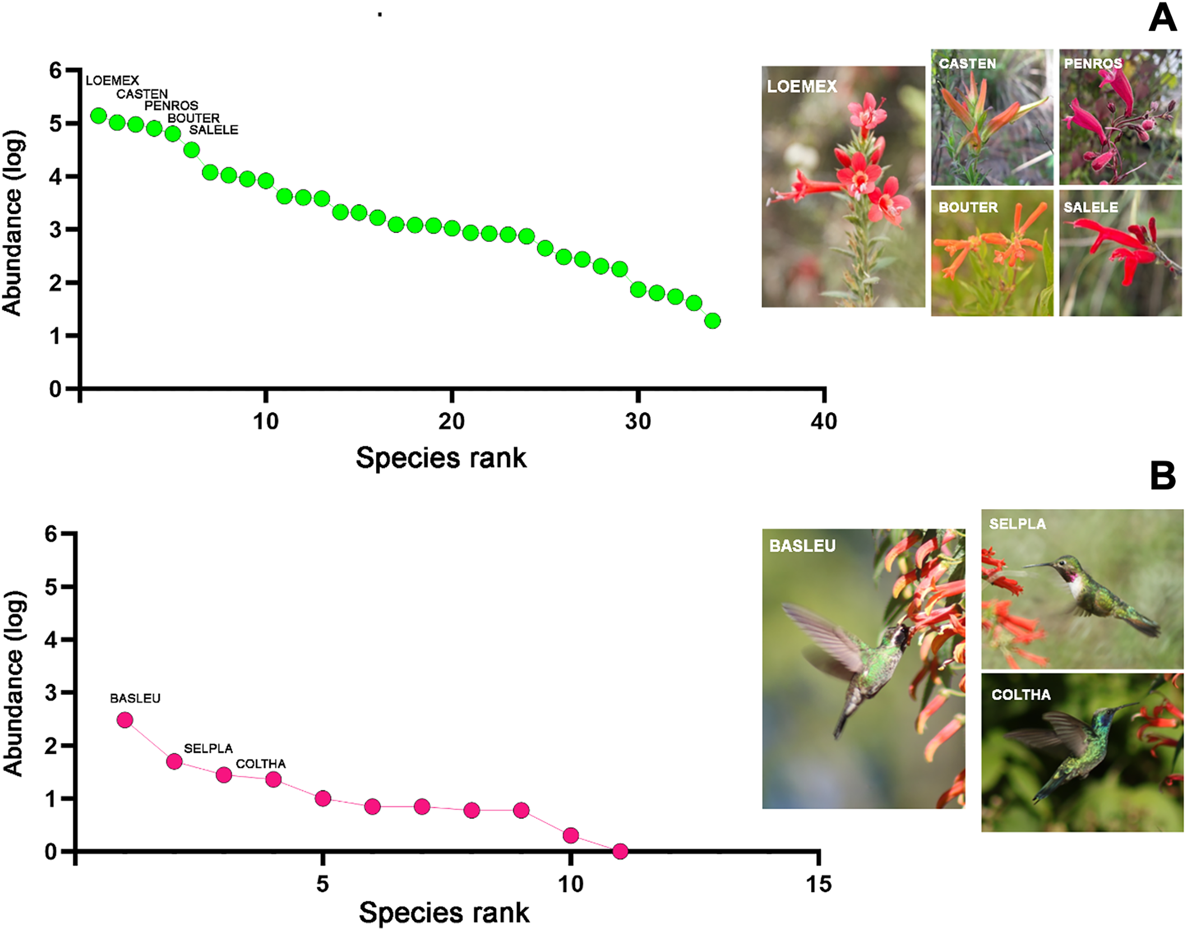
Regarding the hummingbird species, considering all the sampled habitats, a total of 11 species were recorded, classified into nine genera and one family (Trochilidae). In terms of abundance, three hummingbird species comprised 86% of the total abundance. Basilinna leucotis was the most abundant hummingbird species in the region (69%), followed in much lower abundance by Selasphorus platycercus (11%), Colibri thalassinus (6.3%), and Calothorax lucifer (5%). The first three hummingbird species were recorded in all four habitat types, while C. lucifer was only recorded in xerophytic shrubland (File S2, Fig. 2B).
The abundances of the aforementioned plant and hummingbird species exhibited high heterogeneity among the studied habitats (Figs. 3A, 3B, 4A and 4B). For example, L. mexicana was the most abundant plant species in the sampled sites of juniper forest and oak forest, but scarce in pine forest and xerophytic shrubland. C. tenuiflora was particularly abundant in xerophytic shrubland, but recorded with low abundance in the other habitats. B. ternifolia was abundant in juniper forest, xerophytic shrubland and oak forest, but not in pine forest. In pine forest, both P. roseus and S. elegans were abundant species. In contrast, in oak forest, the abundance of both species was low, while in juniper forest and xerophytic shrubland they were not recorded (File S2, Figs. 3A and 4A).
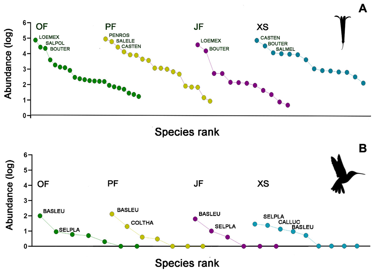
Figure 3: Rank/abundance plots for the hummingbirds and their flowering plant species by each sampled habitat type.
(A) Loeselia mexicana (LOEMEX), Castilleja tenuiflora (CASTEN), Penstemon roseus (PENROS), Bouvardia ternifolia (BOUTER), Salvia elegans (SALELE), S. polystachya (SALPOL) and S. melissodora (SALMEL) were the most abundant plant species in each sampled habitat type: Oak forest (OF), pine forest (PF), juniper forest (JF), and xerophytic shrubland (XS), while (B) Basilinna leucotis (BASLEU), Selasphorus platycercus (SELPLA), Colibri thalassinus (COLTHA) and Calothorax lucifer (CALLUC) highly dominate in all sampled habitat types. The hummingbird silhouette used in Figs. 3–6 was obtained from an open source platform (https://www.phylopic.org/images/2bf1e800-5384-45cd-a533-ac940b8eadd6/trochilidae) and created by Ferran Sayol. The flower silhouette in these figures was created by the authors using Adobe Photoshop 7.0 software (Adobe Inc., San Jose, CA, USA).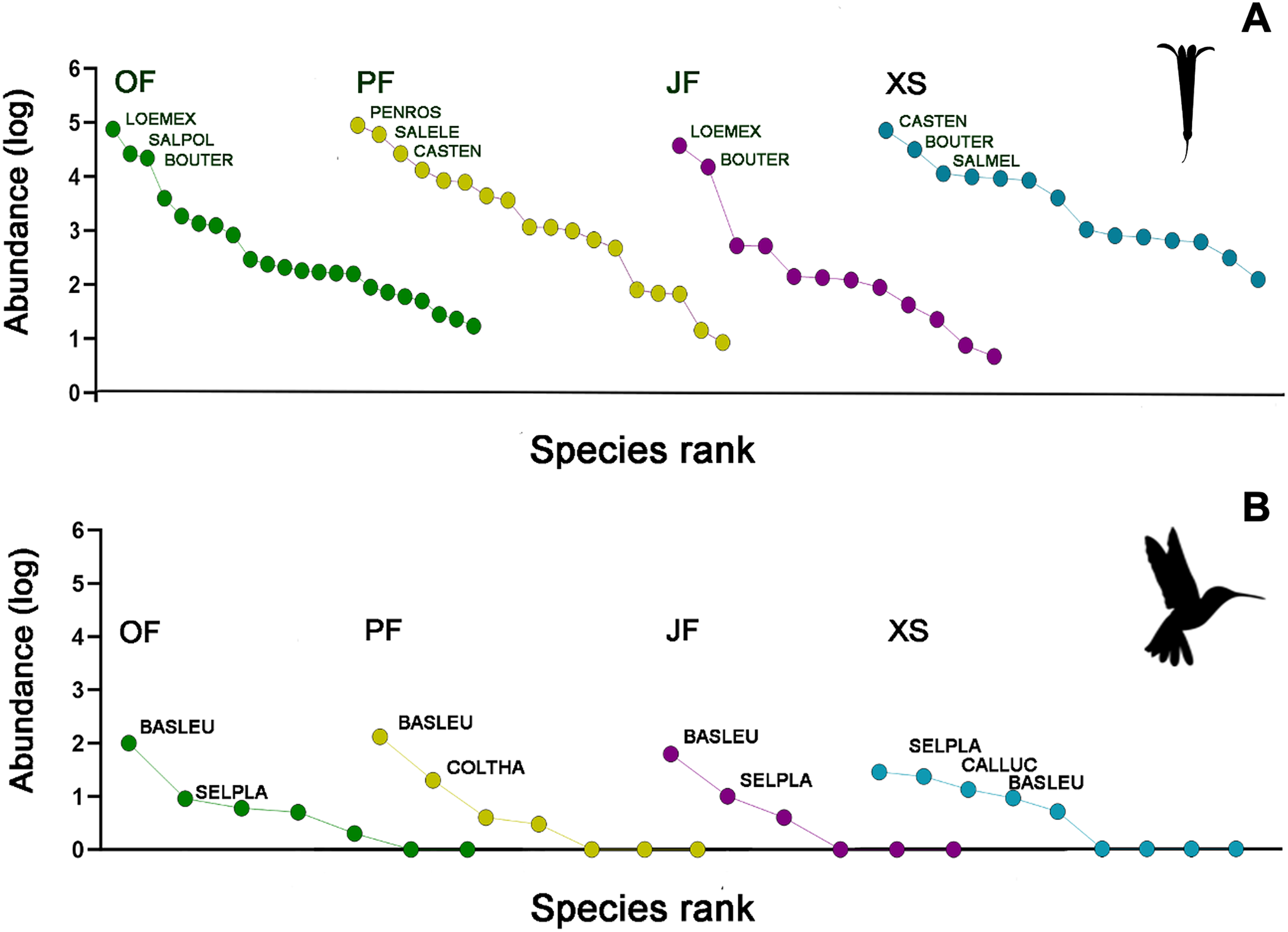
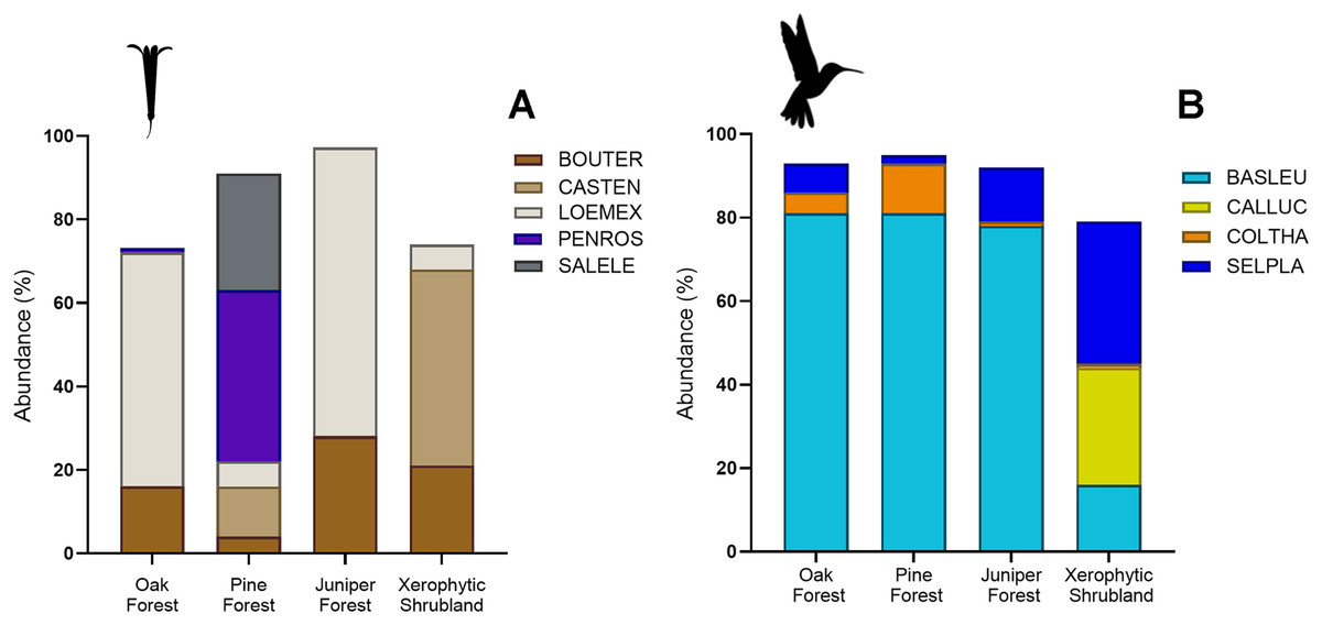
Figure 4: Relative abundance (%) of key plant and hummingbird species across different forest types.
(A) Percentage of herbaceous plant species: Bouvardia ternifolia (BOUTER), Castilleja tenuiflora (CASTEN), Loeselia mexicana (LOEMEX), Penstemon roseus (PENROS), and Salvia elegans (SALELE). (B) Percentage of hummingbird species: Basilinna leucotis (BASLEU), Calothorax lucifer (CALLUC), Colibri thalassinus (COLTHA), and Selasphorus platycercus (SELPLA).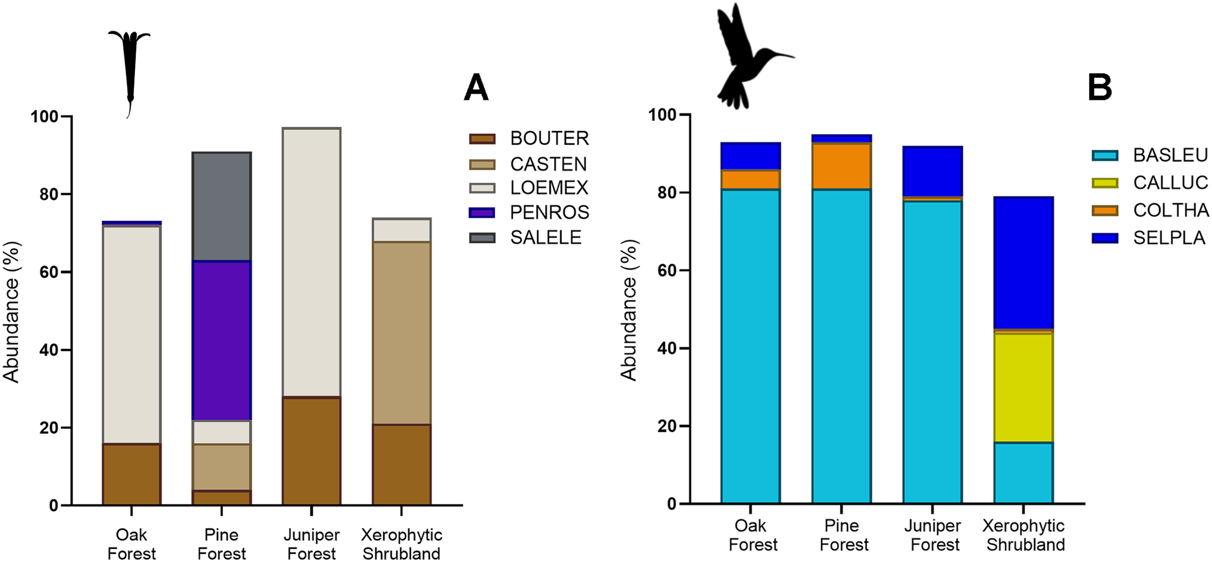
Hummingbird species abundances were also highly variable among the sampled habitats. B. leucotis was the most abundant species in pine forest, oak forest, and juniper forest, while less abundant in xerophytic shrubland. Conversely, S. platycercus was the most abundant in xerophytic shrubland, and less abundant in other habitats. C. thalassinus was one of the most abundant species in pine forest and showed very low abundances in the remaining habitat types. Finally, C. lucifer was an abundant species found exclusively in the xerophytic shrubland habitat (File S2, Figs. 3B and 4B).
Diversity measures
Richness at regional level of plants was 34 species (0Dγ), with an average local richness (0Dα) of 16.5 effective species and 2.06 effective communities (0Dβ) necessary to account the regional species richness within the region. This implies that on average, 48.5% (1/0Dβ) of the total plant species are present in a single habitat. For hummingbird assemblages, the average richness (0Dα) was 7.3 effective species, representing 66.6% of the total species recorded within the region (0Dγ = 11). With a 0Dβ of 1.5 effective communities needed to achieve regional richness, it suggests minimal species turnover within the region. Considering the effective communities in hummingbirds, the species recorded in xerophytic shrubland (nine spp.) and oak forest (two spp.) contribute to completing the regional richness (Table 1).
| Gamma diversity | ||||
|---|---|---|---|---|
| Dγ diversity and its components |
Hummingbirds | Flowering Plants | ||
| 0D | 1D | 0D | 1D | |
| Dγ | 11 | 3.3 | 34 | 8.7 |
| Dβ | 1.5 | 1.3 | 2.06 | 2 |
| Dα | 7.3 | 2.5 | 16.5 | 4.4 |
Note:
Dα and Dγ are expressed in the same units of species, while Dβ is expressed in communities. Superscripts correspond to diversity values of orders 0 and 1, based on Hill numbers representing the effective number of species or communities.
In terms of the regional diversity 1Dα (equiprobable species) in the plants, an average community calculated 4.4 effective species, while 8.7 effective species were observed in the entire region (1Dγ). The communities required to complement 1Dγ are 2 (1Dβ), indicating that an average community contained 50% of the equiprobable species in the region. For the hummingbird assemblages, an average community displayed 2.5 effective species (1Dα), and the region exhibited 3.3 effective species (1Dγ). To complement 1Dγ, 1.3 communities were required (1Dβ), with an average community encompassing 77% of the equiprobable species in the region (Table 1). Regional diversity (1Dγ) aligned closely with the abundant species recorded within the region (Fig. 2).
Regarding alpha diversity (α), the habitat with the highest richness (0D) of plant species was oak forest (22 species), followed by pine forest (18 species), and xerophytic shrubland (14 species). Juniper forest (12 species) had the lowest richness, with the lowest number of effective species of 1D (2.1) and 2D (1.8), particularly recording two dominant species (L. mexicana and B. ternifolia) (Fig. 3B). In contrast, habitats with the highest number of effective species in orders 1 and 2 are pine forest (1D = 5.3, 2D = 3.8) and xerophytic shrubland (1D = 5.2, 2D = 3.5), respectively (Fig. 5B; Table 2). Consequently, in terms of order 1 diversity, on average, pine forest and xerophytic shrubland exhibited 2.5 times more diverse than juniper forest and 1.4 times more diverse than oak forest. Pine forest presented the five most abundant species within the region (P. roseus, S. elegans, C. ternuiflora, L. mexicana, B. ternifolia) (Fig. 2B), while xerophytic shrubland shared three species with pine forest (C. ternuiflora, B. ternifolia, L. mexicana) and had two exclusive abundant species (Salvia chamaedryoides and Salvia melissodora) (File S2).
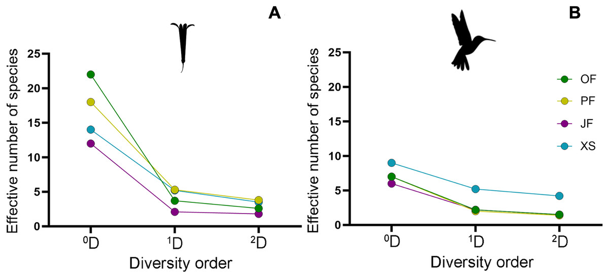
Figure 5: Alpha diversity profiles of hummingbirds and their flowering plant species in the four sampled habitat types.
By following the true diversity concept (Jost, 2006), we obtained the diversity profiles for (A) plants and (B) hummingbirds, showing variation in the number of effective species for each sampled habitat type: Oak forest (OF), pine forest (PF), juniper forest (JF), and xerophytic shrubland (XS). Superscripts correspond to diversity values of orders 0, 1, and 2; values for orders 1 and 2 are shown as Hill numbers, representing the effective number of species.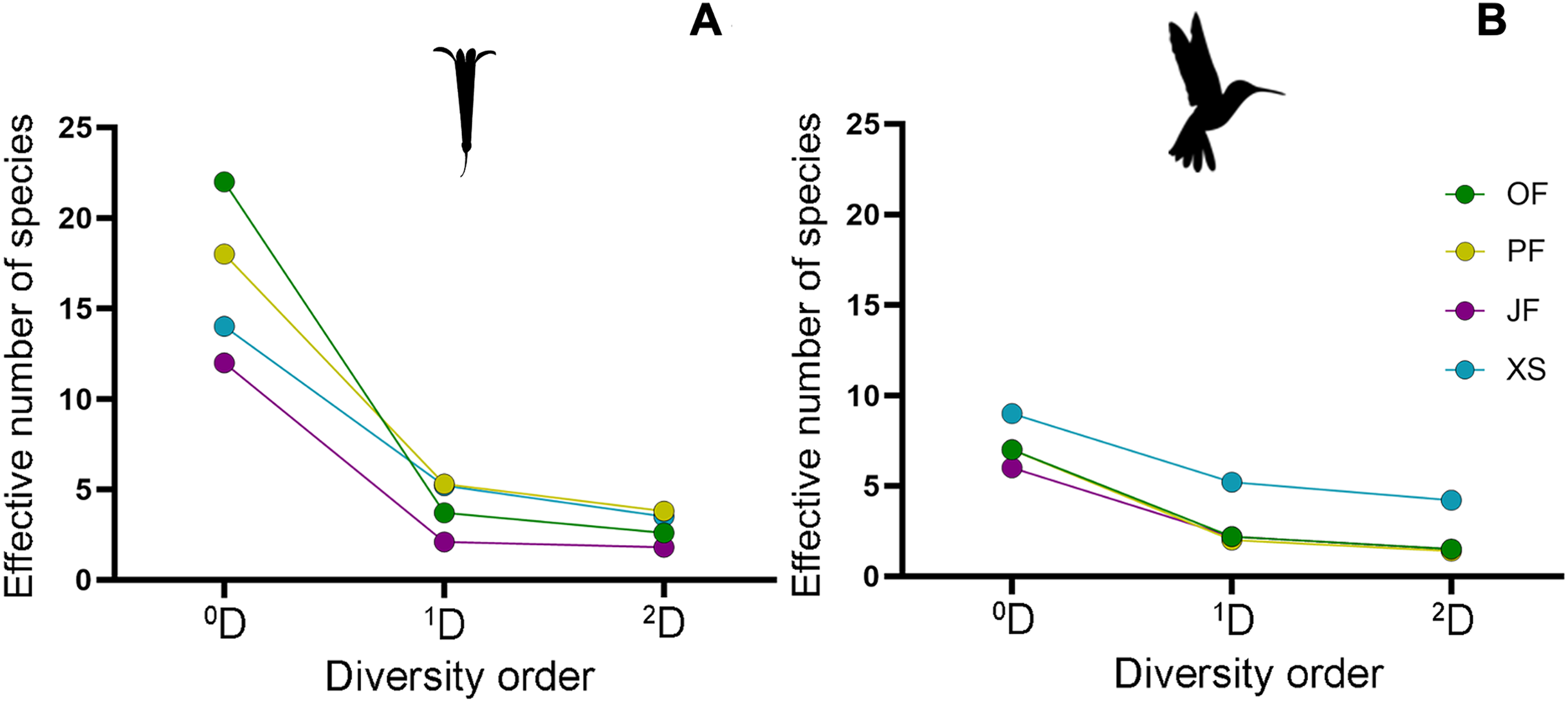
| Alpha diversity | ||||||
|---|---|---|---|---|---|---|
| Hummingbirds | Flowering plants | |||||
| Habitat type | 0D | 1D | 2D | 0D | 1D | 2D |
| OF | 7 | 2.2 | 1.5 | 22 | 3.7 | 2.6 |
| PF | 7 | 2 | 1.4 | 18 | 5.3 | 3.8 |
| JF | 6 | 2.2 | 1.5 | 12 | 2.1 | 1.8 |
| XS | 9 | 5.2 | 4.2 | 14 | 5.2 | 3.5 |
Note:
Superscripts correspond to diversity values of orders 0, 1, and 2, represented by Hill numbers, reflecting the effective number of species.
The habitat with the highest diversity of hummingbird species was xerophytic shrubland, recording the highest richness (0D = 9) and the greatest number of effective species (1D = 5.2, 2D = 4.2). In this habitat, five abundant hummingbird species were found, two of which ranked among the most abundant species in the region, and one was exclusive to xerophytic shrubland (B. leucotis, S. platycercus, S. rufus, A. colubris, and C. lucifer, respectively) (Fig. 3A). In contrast, the lowest diversity of hummingbird species was observed in oak forest, pine forest, and juniper forest, with assemblages having a similar number of effective species. Considering the order 1 diversity measure, the xerophytic shrubland was, on average, 2.77 times more diverse than the other habitat types (Fig. 5A; Table 2).
Beta diversity (β)
The βcc values obtained among the plant communities indicate dissimilarity ranging from 0.52 to 0.77 (where 1 represents maximum dissimilarity). Xerophytic shrubland is dissimilar compared to the other three habitats (>0.70) (Table 3). The dissimilarity among all communities is primarily attributed to species turnover (β-turnover), except in oak forest vs. juniper forest, where dissimilarity is attributed to differences in richness (β-nestedness) (Fig. 6A; Table 3). The hummingbird communities have dissimilarity ranging from 0.38 to 0.56. Overall, dissimilarity is driven by species turnover (Fig. 6B; Table 3). When evaluating the beta diversity between pairs of sites, a very similar trend was found for plants and hummingbirds, where the dissimilarity was mainly due to β-turnover, with low contribution in β-nestedness. However, the highest values of total beta (βcc) between habitats occurred in plant communities, while lower values were observed in hummingbird assemblages, indicating greater similarity in hummingbird species composition between habitats (Figs. 6A and 6B).
| Beta diversity | ||||||
|---|---|---|---|---|---|---|
| Hummingbirds | Flowering plants | |||||
| Habitat type | β-turnover | β-nestedness | βcc | β-turnover | β-nestedness | βcc |
| OF vs. JF | 0.25 | 0.13 | 0.38 | 0.09 | 0.43 | 0.52 |
| OF vs. PF | 0.44 | 0 | 0.44 | 0.43 | 0.14 | 0.57 |
| OF vs. XS | 0.36 | 0.18 | 0.55 | 0.43 | 0.29 | 0.71 |
| JF vs. PF | 0.44 | 0.11 | 0.56 | 0.50 | 0.25 | 0.75 |
| JF vs. XS | 0.20 | 0.30 | 0.50 | 0.60 | 0.10 | 0.70 |
| PF vs. XS | 0.20 | 0.20 | 0.40 | 0.62 | 0.15 | 0.77 |
Note:
This analysis was carried out across four sampled habitat types: oak forest (OF), pine forest (PF), juniper forest (JF), and xerophytic shrubland (XS).
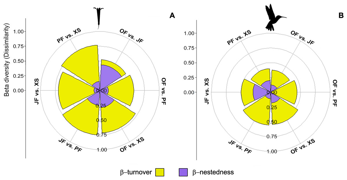
Figure 6: Contribution of species turnover and differences in species richness to beta diversity of hummingbirds and flowering plants.
Plots show beta diversity of (A) plant and (B) hummingbird species, where each segment shows the proportion of each component for each habitat pair: Oak forest (OF), pine forest (PF), juniper forest (JF), and xerophytic shrubland (XS).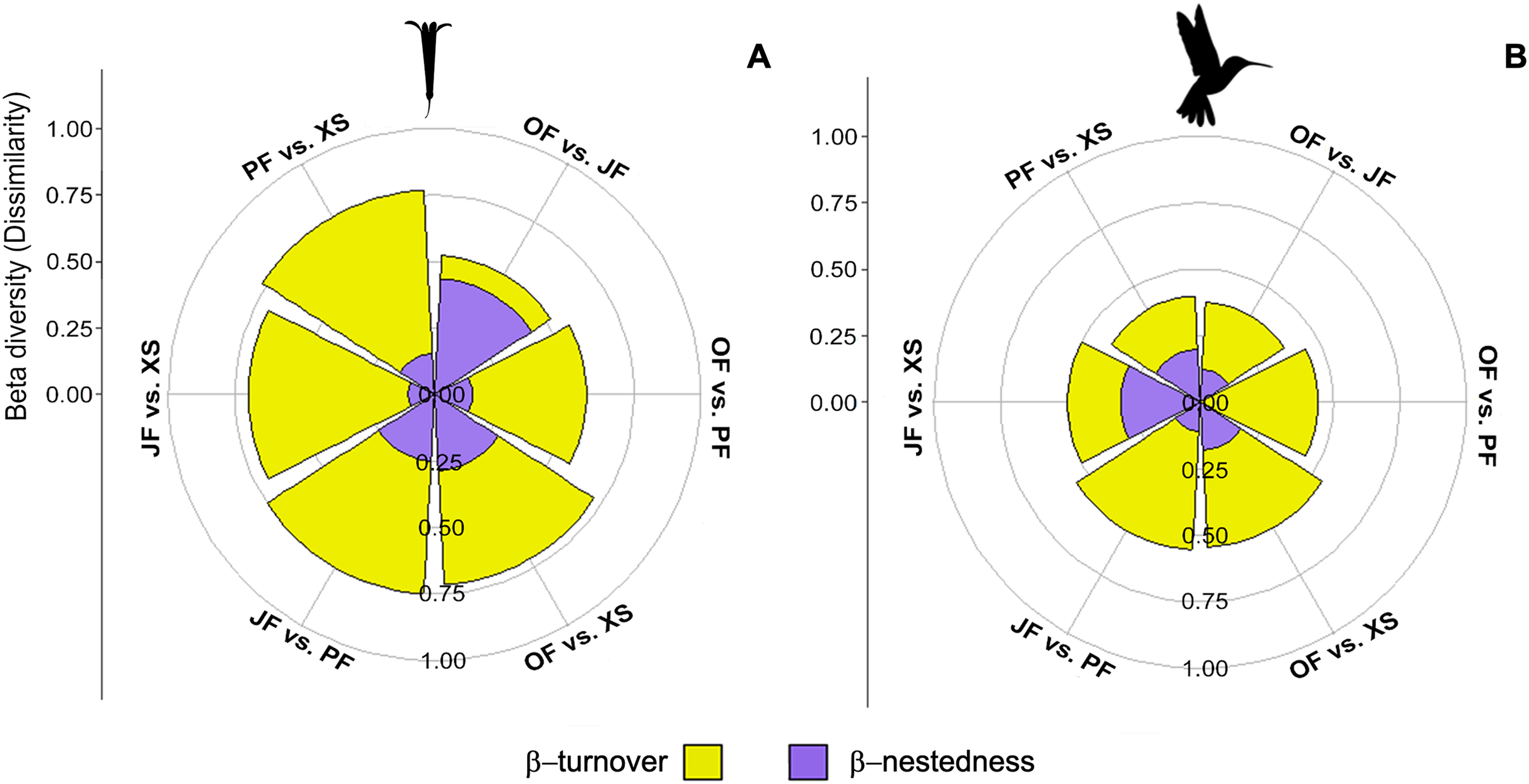
The relationship between beta diversity and environmental factors
Mantel’s simple and partial tests for plant species, between the beta components and selected environmental factors in the study, showed a positive correlation in βcc dissimilarities with the climate variables precipitation (Bio12), precipitation of wettest quarter (Bio16), and altitude ranging from r = 0.34 to r = 0.45. Partial correlations confirm that climate variables contribute more in the relationship. Similar results were obtained for species turnover (β-turnover), with correlation coefficients ranging from r = 0.27 to r = 0.4 (Table 4). In summary, we found variation in the species turnover rate for both measured variables (altitude and climate variables). However, environmental conditions had a greater effect on the dissimilarity of plant species assemblages. For hummingbird species assemblages, differences in βcc and β-turnover are explained by climate variables (r = 0.45) and not by altitude (Table 4). Correlations for richness differences (β-nestedness) were not significant in either case (plants and hummingbirds).
| Hummingbirds | ||||||||
|---|---|---|---|---|---|---|---|---|
| Altitude | Climate variables | Climate variables-altitude | Altitude-climate variables | |||||
| r | p | r | p | r | p | r | p | |
| βcc | −0.01 | 0.50 | 0.45 | <0.01 | 0.45 | <0.01 | 0.03 | 0.41 |
| β-turnover | −0.20 | 0.91 | 0.31 | <0.01 | 0.30 | <0.01 | −0.19 | 0.90 |
| β-nestedness | 0.22 | 0.13 | 0.01 | 0.41 | 0.03 | 0.34 | 0.22 | 0.13 |
| Flowering plants | ||||||||
| βcc | 0.34 | <0.01 | 0.45 | <0.01 | 0.51 | <0.01 | 0.42 | <0.01 |
| β-turnover | 0.27 | 0.01 | 0.40 | <0.01 | 0.44 | <0.01 | 0.33 | <0.01 |
| β-nestedness | −0.05 | 0.54 | −0.12 | 0.93 | −0.12 | 0.94 | −0.06 | 0.57 |
Note:
Dα and Dγ are expressed in the same units of species, while Dβ is expressed in communities. Superscripts correspond to diversity values of orders 0 and 1, based on Hill numbers representing the effective number of species or communities.
Discussion
Our study provides a comprehensive understanding of the abundance, composition, and diversity of flowering plants and hummingbirds across different habitat types in central Tlaxcala, Mexico. The main goal of our research was to unravel the alpha, beta, and gamma diversity patterns within hummingbird-flower communities across the most representative habitats of the region: the oak forest, pine forest, juniper forest, and xerophytic shrubland (Fig. 1). These habitats form gradients of humidity and temperature in the same landscape, ranging from typically humid and cold conditions in the forests to dry and warm environments in the xerophytic shrubland.
As expected, we found significant variations in alpha, beta, and gamma diversity of hummingbird-flower communities across these habitats (Figs. 5 and 6, Tables 1 and 2), confirming that their distinct environmental conditions play a crucial role in shaping species composition and diversity patterns. These findings align with previous studies documenting higher species richness and turnover in habitats with greater environmental heterogeneity (Tuanmu & Jetz, 2014; Socolar et al., 2016). Our results also supported the hypothesis that abiotic factors such as altitude, temperature, and precipitation influence species composition between habitats (beta diversity). We found significant positive correlations between climate variables and dissimilarities in both plant and hummingbird species assemblages (Table 4), highlighting the importance of environmental conditions in structuring these communities (Chase et al., 2011; Belmaker & Jetz, 2015).
Interestingly, we observed a higher turnover of plant species compared to hummingbirds along the studied environmental gradient (Fig. 6, Table 3). This difference may be attributed to the greater mobility of hummingbirds, which allows them to exploit a wider variety of habitats and resources (Hadley & Betts, 2012). In contrast, plants are more limited in their dispersal and distribution due to factors such as substrate availability, competition, and seed dispersal mechanisms (Willson, 1993; Dalling et al., 2002). This finding has important implications for conservation strategies in the region. While hummingbirds demonstrate a degree of habitat generalism, many plant species exhibit specialized associations with specific habitats. Therefore, preserving a mosaic of diverse habitats is crucial to maintain the unique plant assemblages they support and to ensure the availability of resources for hummingbirds across the landscape (Hobbs et al., 2014; Socolar et al., 2016).
The distance among study sites could influence beta diversity patterns by affecting species turnover across habitats, isolation and connectivity of populations, changes in environmental conditions, species dispersal abilities, and broader biogeographic patterns (Soininen, McDonald & Hillebrand, 2007). We addressed this by selecting geographically separated locations (average distance > 13 km) for each habitat type (Fig. 1), allowing for a more nuanced understanding of biodiversity patterns within and among habitat types. However, while our study design considered spatial separation, future research could delve deeper into environmental gradients and landscape connectivity to better understand biodiversity patterns in complex landscapes like those in Tlaxcala, Mexico.
It is important to emphasize that, although our study did not directly quantify the interactions between plants and hummingbirds, the observed patterns in species abundance and distribution (Figs. 2–4) strongly suggest the existence of intricate interaction networks that deserve further exploration in future research (Vázquez et al., 2009; Trøjelsgaard & Olesen, 2013). Understanding these complex ecological relationships is crucial for predicting how changes in the abundance and distribution of one group may affect the other, and for developing effective conservation strategies that consider the interdependence of these species.
The documentation of a diverse array of plant species across multiple taxonomic groups highlights the ecological significance of the floral community in our study area (Potts et al., 2010; Ollerton, Winfree & Tarrant, 2011). The prevalence of five key plant species—Loeselia mexicana, Bouvardia ternifolia, Castilleja tenuiflora, Penstemon roseus, and Salvia elegans—in terms of flower abundance is notable (Figs. 2–4). These species, characterized by red flowers, may occupy key resource positions within the ecosystem, influencing community composition and structure (Paine, 1969; Scogin, 1983). Furthermore, the presence of characteristic plant species shared across all four habitat types underscores their ecological importance and potential role as indicators of habitat health (Lechner, Chan & Campos-Arceiz, 2018).
Within the realm of hummingbird diversity, our study identifies 11 recorded species, categorized into nine genera within the family Trochilidae (Fig. 2). The hummingbird species richness in our study region is relatively higher compared to other temperate forests of North and South America, where up to 13 species may be present (Abrahamczyk & Renner, 2015; López-Segoviano, Bribiesca & Arizmendi, 2018). The resident Basilinna leucotis emerges as the dominant hummingbird species, constituting a substantial 69% of the regional hummingbird population (Figs. 2–4). This dominance can potentially influence plant-hummingbird interactions and pollination dynamics within the ecosystem (Stiles, 1981; Magrach et al., 2020). Interestingly, the second most abundant hummingbird species was the long-distance migrant Selasphorus platycercus, recorded throughout most of the year in all four habitat types (Figs. 2–4). This finding suggests that both resident and winter migratory populations can be found and may even reproduce in these habitats, highlighting the importance of the region for hummingbird conservation.
Our exploration of alpha diversity among different habitats unveils intriguing patterns of species richness and evenness (Fig. 5, Table 2). Habitats such as pine forest and xerophytic shrubland stand out as bastions of high alpha diversity of flowering plants, suggesting the presence of diverse and evenly distributed species assemblages (Grime, 1998). In contrast, juniper forest exhibits lower diversity, beckoning further investigation into the drivers of this pattern, including resource availability and biotic interactions (Connell, 1978; Tilman, 1982). Understanding the variations in alpha diversity among habitats has profound implications for crafting effective land management and conservation strategies. Our findings underscore the imperative to prioritize the protection and restoration of diverse habitats to maintain biodiversity and enhance ecosystem resilience (Noss & Cooperrider, 1994).
The exploration of beta diversity, especially the dissimilarity among plant and hummingbird communities, unveils the uniqueness of species assemblages across habitats (Fig. 6, Table 3). The high dissimilarity observed in xerophytic shrubland points to the existence of distinctive ecological communities, potentially shaped by factors such as dispersal limitation, environmental gradients, or species interactions (Legendre et al., 2009). Additionally, the lower dissimilarity of hummingbird assemblages compared to plants may be attributed to hummingbirds’ higher mobility, enabling them to exploit diverse habitats more readily (Hadley & Betts, 2012). Overall, the dissimilarity in species composition is primarily due to species turnover, implying unique ecological roles and contributions of different species to each habitat. These findings emphasize the paramount importance of preserving a variety of habitats to safeguard the diverse assemblages they harbor.
The computation of gamma diversity (Dγ) and beta diversity (Dβ) provides a quantitative foundation for unraveling the regional biodiversity of plant and hummingbird species (Table 1). These metrics, integral to contemporary ecological research (Chao et al., 2014), lay the groundwork for informed regional biodiversity assessments and conservation planning (Jost et al., 2010). The finding of low species turnover in hummingbird assemblages suggests a degree of stability in the species composition across habitats, while higher turnover in plants reflects the presence of habitat specialists alongside widespread species. This nuanced understanding of species turnover has far-reaching implications for ecosystem connectivity and resilience. The presence of habitat specialists signals unique ecological roles and dependencies within their respective ecosystems, urging conservationists to consider the holistic preservation of habitats (Devictor et al., 2007; Cardinale et al., 2012).
Our study found a significant relationship between environmental factors (specifically climate variables) and dissimilarities in both plant species and hummingbird species assemblages (Table 4). The positive correlation observed in Bcc indicates that as climate variables and altitude vary, the dissimilarity in the composition of plant species increases. Furthermore, the results show that climate variables play a more influential role in this relationship compared to altitude (Table 4). This suggests that the climatic conditions of a habitat are particularly important in shaping the composition of plants. The variations in species turnover (β-turnover) also align with this pattern, reinforcing the impact of environmental conditions on the diversity and composition of plant species. In the case of hummingbird species, the dissimilarities in βcc and β-turnover are mainly influenced by climate variables, not altitude. This emphasizes the significance of climate in determining the composition and diversity of hummingbird species across different habitats.
However, our study did not find significant correlations for richness differences (β-nestedness) for both plant and hummingbird species (Table 4). This implies that differences in species richness between habitats were not strongly related to the measured environmental variables and altitude. Thus, the positive correlations detected between beta diversity and climate variables, offer compelling insights into the potential influence of climate change on species composition within our research region (Bellard et al., 2012). The ramifications of shifting climate conditions extend to alterations in species distributions, impacting ecological dynamics and the provisioning of ecosystem services (Parmesan, 2006).
Previous studies have shown that climate change can be particularly threatening to hummingbirds by affecting the phenology of floral resources on which they depend (Inouye et al., 2000; McKinney et al., 2012). Even minor changes in blooming dates may be of consequence, as hummingbirds will eventually arrive after flowering begins, which could reduce their nesting success (Aldridge et al., 2011; McKinney et al., 2012). This disruption in the flowering phenology within and among different habitats can affect both latitudinal and altitudinal migration undertaken by hummingbirds following these floral resources. The established interaction networks between hummingbirds and their floral resources should be incorporated into future studies of geographic distribution models and climate change. Thus, our findings accentuate the central role played by environmental conditions in shaping species assemblages (Chase et al., 2011). This knowledge informs the development of effective habitat conservation and restoration strategies that account for the influence of climate and topography on ecosystem structure and function (Sax et al., 2007; Hobbs et al., 2014).
Conclusions
Our study provides valuable insights into the diversity patterns and community structuring of flowering plants and hummingbirds across different habitat types in central Tlaxcala, Mexico. The findings underscore the significant influence of environmental factors, particularly climate variables, on shaping the distribution and assembly of these ecologically coupled groups. The higher turnover of plant species compared to hummingbirds highlights the importance of considering species-specific traits, such as dispersal abilities and resource requirements, when developing conservation strategies. While hummingbirds exhibited a degree of habitat generalism, allowing them to exploit multiple habitats, many plant species were more specialized, leading to unique community assemblages across the landscape. Therefore, preserving habitat heterogeneity and landscape connectivity emerges as a key strategy to sustain regional biodiversity and promote ecosystem resilience in the face of environmental change.
Our results emphasize the paramount importance of preserving habitat heterogeneity to safeguard regional biodiversity. Key habitats harboring high species diversity and unique assemblages, such as the xerophytic shrubland and pine forests, should be prioritized for protection. Furthermore, maintaining landscape connectivity is crucial to facilitate the movement and gene flow of more mobile species like hummingbirds.
This study lays the foundation for future research investigating the intricate interaction networks between flowering plants and hummingbirds, and how these ecological relationships may be impacted by environmental changes and anthropogenic disturbances. By considering the complex interplay between species, habitats, and environmental factors, we can develop informed conservation strategies that promote ecosystem resilience and ensure the long-term persistence of these vital ecological partnerships. Ultimately, our findings emphasize the necessity of adopting a holistic approach to biodiversity conservation, one that recognizes the interdependence of species and the importance of preserving diverse habitats to maintain functional and resilient ecosystems. Such an approach is essential for mitigating the ongoing biodiversity crisis and safeguarding the invaluable ecological services provided by these intricate ecological webs.
Supplemental Information
Evaluating the completeness of plant and hummingbird diversity sampling across four habitat types.
The supplemental figures assess the sampling coverage achieved for hummingbird and plant diversity in four distinct habitat types: oak forest (OF), pine forest (PF), juniper forest (JF), and xerophytic shrubland (XS). Fig. 1S illustrates that the sampling methods captured over 95% of the estimated hummingbird species richness in all habitats, with some even exceeding 98%. Similarly, Fig. 2S demonstrates that the sampling coverage for plant diversity was highly comprehensive, recording more than 99% of the expected plant species richness across all four habitat types. These results indicate that the sampling efforts were thorough and representative of the plant and humkingbird communities in each habitat, providing a robust foundation for further ecological analyses and comparisons.
The raw measurements used for our analyses.
The study locations, hummingbirds and floral plants abundances, alpha, beta and gamma diversity values, true diversity measures and the climate variables used in the analyses.