

Can we measure beauty? Computational evaluation of coral reef aesthetics
- Published
- Accepted
- Received
- Academic Editor
- Robert Costanza
- Subject Areas
- Computational Science, Environmental Sciences, Natural Resource Management
- Keywords
- Image analysis, Coral reef, Aesthetics, Machine learning, Reef degradation
- Copyright
- © 2015 Haas et al.
- Licence
- This is an open access article distributed under the terms of the Creative Commons Attribution License, which permits unrestricted use, distribution, reproduction and adaptation in any medium and for any purpose provided that it is properly attributed. For attribution, the original author(s), title, publication source (PeerJ) and either DOI or URL of the article must be cited.
- Cite this article
- 2015. Can we measure beauty? Computational evaluation of coral reef aesthetics. PeerJ 3:e1390 https://doi.org/10.7717/peerj.1390
Abstract
The natural beauty of coral reefs attracts millions of tourists worldwide resulting in substantial revenues for the adjoining economies. Although their visual appearance is a pivotal factor attracting humans to coral reefs current monitoring protocols exclusively target biogeochemical parameters, neglecting changes in their aesthetic appearance. Here we introduce a standardized computational approach to assess coral reef environments based on 109 visual features designed to evaluate the aesthetic appearance of art. The main feature groups include color intensity and diversity of the image, relative size, color, and distribution of discernable objects within the image, and texture. Specific coral reef aesthetic values combining all 109 features were calibrated against an established biogeochemical assessment (NCEAS) using machine learning algorithms. These values were generated for ∼2,100 random photographic images collected from 9 coral reef locations exposed to varying levels of anthropogenic influence across 2 ocean systems. Aesthetic values proved accurate predictors of the NCEAS scores (root mean square error < 5 for N ≥ 3) and significantly correlated to microbial abundance at each site. This shows that mathematical approaches designed to assess the aesthetic appearance of photographic images can be used as an inexpensive monitoring tool for coral reef ecosystems. It further suggests that human perception of aesthetics is not purely subjective but influenced by inherent reactions towards measurable visual cues. By quantifying aesthetic features of coral reef systems this method provides a cost efficient monitoring tool that targets one of the most important socioeconomic values of coral reefs directly tied to revenue for its local population.
Introduction
Together with fishing, cargo shipping, and mining of natural resources, tourism is one of the main economic values to inhabitants of coastal areas. Tourism is one of the world’s largest businesses (Miller & Auyong, 1991) and with ecotourism as the fastest growing form of it worldwide (Hawkins & Lamoureux, 2001) the industry is increasingly dependent on the presence of healthy looking marine ecosystems (Peterson & Lubchenco, 1997). In this context coral reefs are one of the most valuable coastal ecosystems. They attract millions of visitors each year through their display of biodiversity, their abundance of colors, and their sheer beauty and lie at the foundation of the growing tourism based economies of many small island developing states (Neto, 2003; Cesar, Burke & Pet-Soede, 2003).
Over the past decades the problem of coral reef degradation as a result of direct and indirect anthropogenic influences has been rigorously quantified (Pandolfi et al., 2003). This degradation affects not only the water quality, but also the abundance and diversity of the reefs inhabitants, like colorful reef fish and scleractinian corals. To assess the status of reef communities and to monitor changes in their composition through time, a multitude of monitoring programs have been established, assessing biophysical parameters such as temperature, water quality, benthic cover, and fish community composition (e.g., Jokiel et al., 2004; Halpern et al., 2008; Kaufman et al., 2011). These surveys however target exclusively on provisioning, habitat, and regulating ecosystem services and neglect their cultural services; i.e., the immediately nonmaterial benefits people gain from ecosystems (Seppelt et al., 2011; Martin-Lopez et al., 2012; Casalegno et al., 2013). Monitoring protocols to assess the biogeochemical parameters of an ecosystem, which need to be conducted by trained specialists to provide reliable data, will not give account of one of the most valuable properties of coastal environments: their aesthetic appearance to humans, which is likely the main factor prompting millions of tourists each year to visit these environments.
The value of human aesthetic appreciation for ecosystems has been studied in some terrestrial (e.g., Hoffman & Palmer, 1996; Van den Berg, Vlek & Coeterier, 1998; Sheppard, 2004; Beza, 2010; De Pinho et al., 2014) and marine ecosystems (Fenton & Syme, 1989; Fenton, Young & Johnson, 1998; Dinsdale & Fenton, 2006). However most of these studies have relied on surveys, collecting individual opinions on the aesthetic appearance of specific animals or landscapes and are therefore hard to reproduce in other locations due to a lack of objective and generalizable assessments of aesthetic properties. A recent approach by Casalegno et al. (2013) objectively measures the perceived aesthetic value of ecosystems by quantifying geo-tagged digital photographs uploaded to social media resources.
Although relatively new in the context of ecosystem evaluation, efforts to define universally valid criteria for aesthetic principles have been existing since antiquity (e.g., Plato, Aristotle, Confucius, Laozi). Alexander Gottlieb Baumgarten introduced aesthetics in 1735 as a philosophical discipline in his Meditationes (Baumgarten & Baumgarten, 1735) and defined it as the science of sensual cognition. Classicist philosophers such as Immanuel Kant, Georg Wilhelm Friedrich Hegel, or Friedrich Schiller, then established further theories of the “aesthetic,” coining its meaning as a sense of beauty and connecting it to the visual arts. Kant (1790) also classified judgments about aesthetic values as having a subjective generality. In the 20th and 21st century, when beauty was not necessarily the primary sign of quality of an artwork anymore, definitions of aesthetics and attempts to quantify aesthetic values have reemerged as a topic of interest for philosophers, art historians, and mathematicians alike (e.g., Datta et al., 2006; Onians, 2007).
With the term aesthetics recipients usually characterize the beauty and pleasantness of a given object (Dutton, 2006). There are however various ways in which aesthetics is defined by different people as focus of interest and aesthetic values may change depending on previous attainment (Datta et al., 2006). For example, while some people may simply judge an image by the pleasantness to the eye, another artist or professional photographer may be looking at the composition of the object, the use of colors and light, or potential additional meanings conveyed by the motive (Datta et al., 2006). Thus assessing the aesthetic visual quality of paintings seems, at first, to pose a highly subjective task (Li & Chen, 2009). Contrary to these assumptions, various studies successfully applied mathematical approaches to determine the aesthetic values of artworks such as sculptures, paintings, or photographic images (Datta et al., 2006; Li & Chen, 2009; Ke, Tang & Jing, 2006). The methods used are based on the fact that certain objects or certain features in them have higher aesthetic quality than others (Datta et al., 2006; Li & Chen, 2009). The overarching consensus hereby is that objects, or images, which are pleasing to the eye, are considered to be of higher value in terms of their aesthetic beauty. The studies which inspired the metrics used in our current work successfully extracted distinct features based on the intuition that they can discriminate between aesthetically pleasing and displeasing images. By constructing high level semantic features for quality assessment these studies have established a significant correlation between various computational properties of photographic images and their aesthetics perceptions by humans (Datta et al., 2006; Li & Chen, 2009).
Methods
Study sites: Four atolls across a gradient of human impact served as basis for this study. The 4 islands are part of the northern Line Islands group located in the central Pacific. The most northern atoll Kingman has no population and is, together with Palmyra which is exposed to sparse human impact, part of the US national refuge system. The remaining two atolls Tabuaeran and Kiritimati are inhabited and part of the Republic of Kiribati (Dinsdale et al., 2008; Sandin et al., 2008). To extend the validity of the method proposed here to other island chains and ocean systems we included an additional sampling site in the Central Pacific (Ant Atoll) and four locations in the Caribbean also subjected to different levels of human impact (2 sites on Curacao, Klein Curacao, and Barbuda, Fig. 1). From every location we collected sets of 172 ± 17 benthic photo-quadrant (Preskitt, Vroom & Smith, 2004) and 63 ± 9 random pictures. To evaluate the level of human impact and status of the ecosystem we used the cumulative global human impact map generated by the National Center for Ecological Analysis and Synthesis (NCEAS; http://www.nceas.ucsb.edu/globalmarine/impacts). These scores incorporate data related to: artisanal fishing; demersal destructive fishing; demersal non-destructive, high-bycatch fishing; demersal non-destructive low-bycatch fishing; inorganic pollution; invasive species; nutrient input; ocean acidification; benthic structures; organic pollution; pelagic high-bycatch fishing; pelagic low-bycatch fishing; population pressure; commercial activity; and anomalies in sea surface temperature and ultraviolet insolation (Halpern et al., 2008; McDole et al., 2012). Additionally, bacterial cell abundance across the 4 Northern Line Islands and 3 of the Caribbean locations (Curacao main island and Barbuda; Table 1) were measured after the method described by Haas et al. (2014).
Aesthetic feature extraction: In total we extracted, modified, and complemented 109 features (denoted as f1, f2,…, f109) from three of the most comprehensive studies on computational approaches to aesthetically evaluate paintings and pictures (Table S1; Datta et al., 2006; Li & Chen, 2009; Ke, Tang & Jing, 2006). Aesthetic evaluation of paintings and photographs in all three studies were based on surveys of randomly selected peer groups. Some of the features presented in previous work were however difficult to reproduce owing to insufficient information given on these features (e.g., f16–24, or f51). This may have led to slight alterations in some of the codes which were inspired by the suggested features but deviate slightly in their final form. As the pictures were considered to be objective samples representing the respective seascape, some traditional aesthetic features, like size of an image or its aspect ratio have not been considered in this study. Overarching feature groups considered in the picture analysis were color, texture, regularity of shapes, and relative sizes and positions of objects in each picture.
Aesthetic value: Although some of the implemented codes appeared similar and were assessing closely related visual aspects, all of the suggested codes were implemented and their value, or potential redundancy, was evaluated using machine learning algorithms. Following feature extraction the 109 feature values were used as input for feed forward neural networks that optimize the importance of features or feature groups and generate a single aesthetic value for each respective photograph. The target outputs for the training of the networks were the NCEAS scores of the regions where the pictures were taken. The pictures were randomly separated into a batch used for training the machine learning algorithms (N = 1,897) and one on which the algorithms were tested (N = 220, 20 from each of 11 sites). We used Matlab’s neural network package on the training samples which further subdivided these samples into training (70%), validation (15%) and test (15%) sets (see Appendix for details). Unlike previous studies in which the aesthetic quality was classified in given categories, this machine learning regression approach generates a continuous metric for the aesthetic quality of a given reefscape.
Results
An aesthetic value of coral reef images was defined using features previously created for measuring the aesthetic quality of images. The values were calibrated using machine learning to match NCEAS scores as closely as possible. Our algorithm gleaned the NCEAS score from an image to within a root mean squared (rms) error of 6.57. Using five images from the same locale improved the NCEAS score prediction to an rms error of 4.46. The relative importance for each feature derived from a random forests approach showed that all three overarching feature groups, texture, color of the whole image, and the size, color, and distribution of objects within an image yielded important information for the algorithm (Fig. S1). The ten most important features, or feature groups were hereby the similarity in spatial distribution of high frequency edges, the wavelet features, number of color based cluster, the area of bounding boxes containing a given percentage of the edge energy, the average value of the HSV color space, entropy of the blue matrix, range of texture, the arithmetic and the logarithmic average of brightness, and the brightness of the focus region as defined by the rule of thirds.
The mean coral reef aesthetic values generated with this approach for each picture were significantly different (p < 0.001) between all sampling locations except for Ant Atoll, Fanning and Klein Curacao (ANOVA followed by Tukey, see Table S2). These sites are also exposed to comparable levels of anthropogenic disturbance (NCEAS: 14.11–19.48). Regression of coral reef aesthetic values against the NCEAS scores of the respective sampling site showed a significant correlation (p < 0.001) for both the training (n = 1,897, R2 = 0.93) and the test (n = 220, R2 = 0.80) set of images (Fig. 2). Further comparison to microbial abundance, available for 7 of the 9 locations (microbial numbers for Curacao Buoy2 and Ant Atoll were not available), revealed a significant correlation between the aesthetic appearance of the sampling sites and their microbial density (p = 0.0006, R2 = 0.88; Fig. 3).
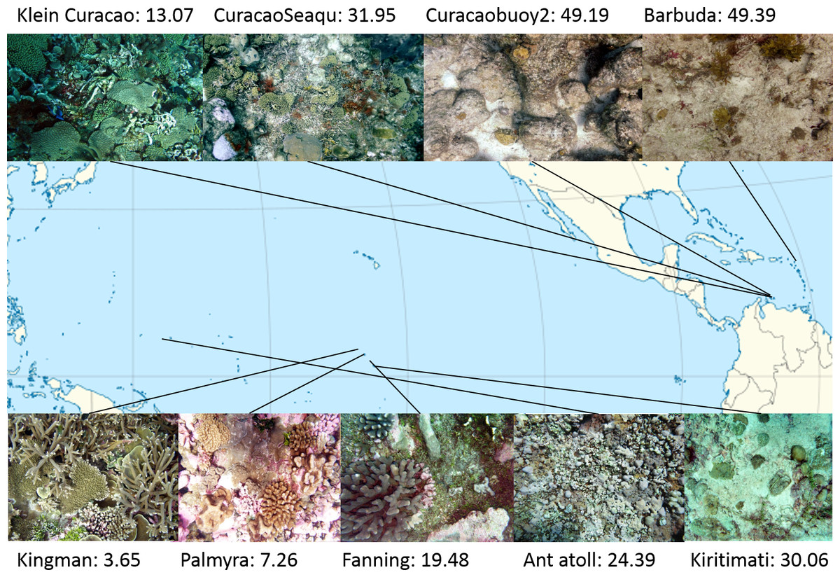
Figure 1: Map of sampling sites with representative images and NCEAS scores.
The upper 4 images show images of the benthic community in the respective Caribbean sites, the lower images represent the sampling sites throughout the tropical Pacific.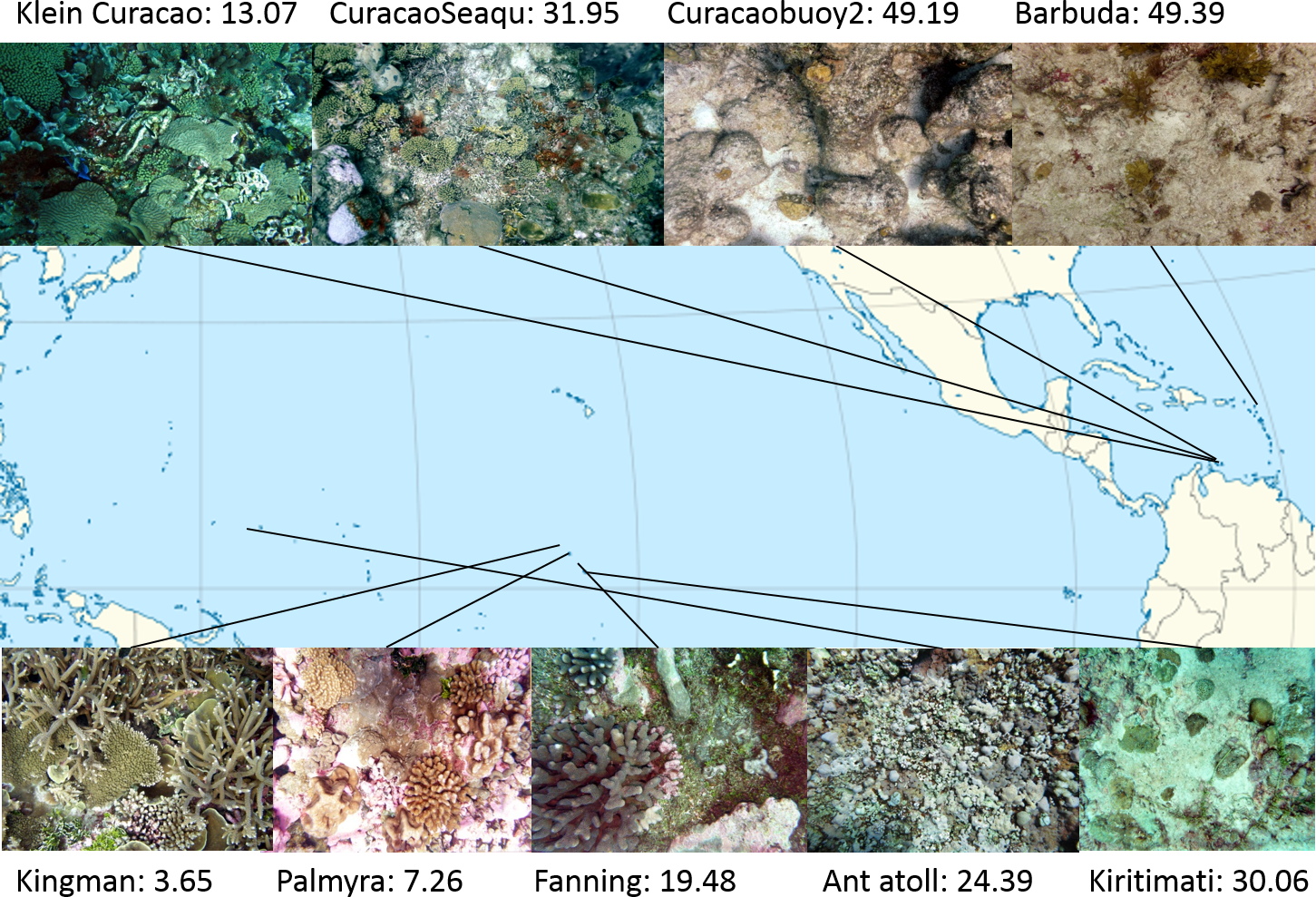
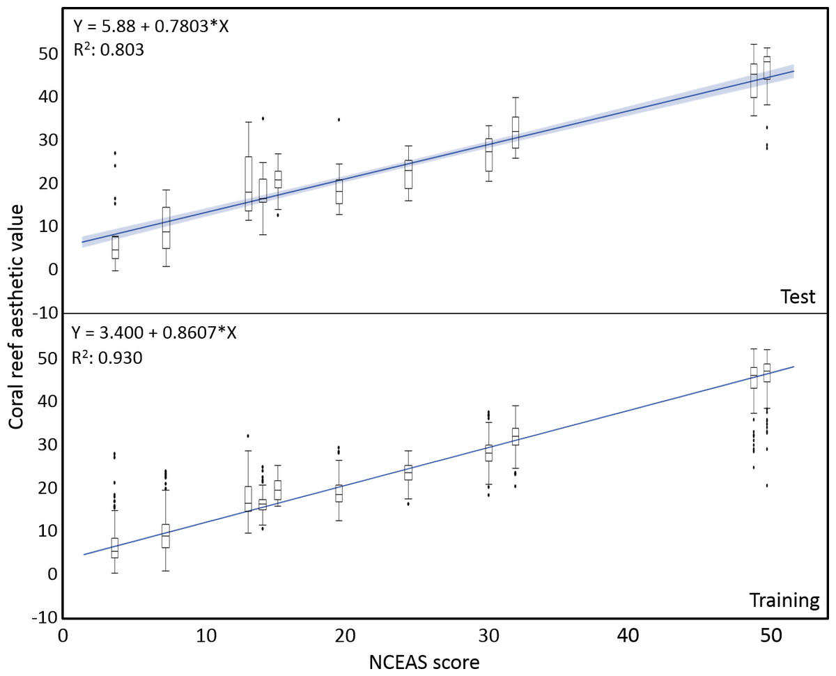
Figure 2: Coral reef aesthetic values.
Boxplots of coral reef aesthetic values at each site and regression of coral reef aesthetic values vs. NCEAS scores across all assessed reef sites. (Test) shows coral reef aesthetic values calculated for 200 images on which the previously trained machine learning algorithm was tested. (Training) shows the generated coral reef aesthetic values from 1,970 images used to improve the feed forward neural networks that optimized the importance of features or feature groups in generating a single coral reef aesthetic value.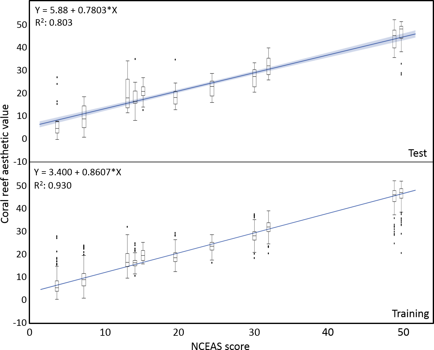
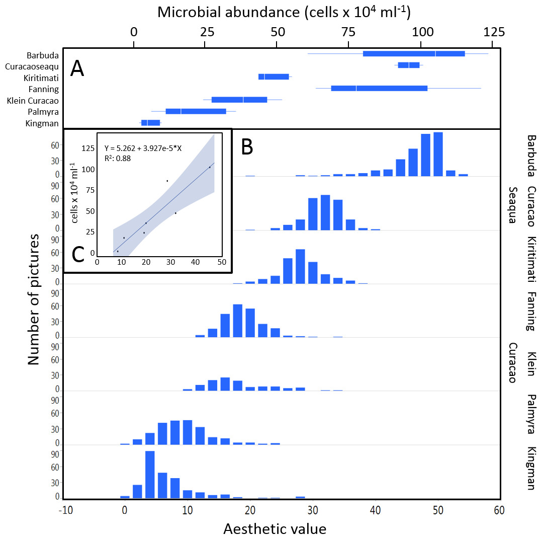
Figure 3: Distribution of aesthetic values.
(A) shows microbial cell abundance at 7 reef sites. (B) shows the distribution of pictures with respective aesthetic values at each of those sites. (C) shows the regression between mean microbial cell abundance and mean aesthetic value (training + test) across all 7 sampling sites.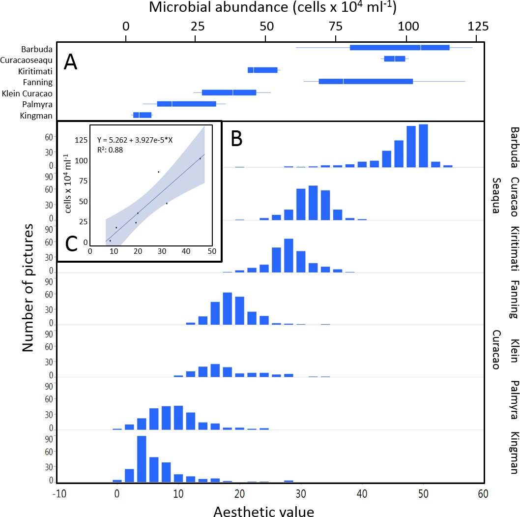
Discussion
This is the first study using standardized computational approaches to establish a site-specific correlation between aesthetic value, ecosystem degradation, and the microbialization (McDole et al., 2012) of marine coral reef environments.
Human response to visual cues
The connection between reef degradation and loss of aesthetic value for humans seems intuitive but initially hard to capture with objective mathematical approaches. Dinsdale (2009) showed that human visual evaluations provided consistent judgment of coral reef status regardless of their previous knowledge or exposure to these particular ecosystems. The most important cue was the perceived health status of the system. Crucial for this intuitive human response to degraded or “unhealthy” ecosystems is the fact that we are looking at organic organisms and react to them with the biological innate emotion of disgust (Curtis, 2007; Hertz, 2012). Being disgusted is a genetically anchored reaction to an object or situation, which might be potentially harmful to our system. Often, a lack of salubriousness of an object or situation is the crucial element for our senses, one of them visual perception, to signal us to avoid an object or withdraw from a situation (Foerschner, 2011). As the microbial density and the abundance of potential pathogens in degrading reefs are significantly elevated (Dinsdale et al., 2008)—albeit not visible to the human eye—our inherent human evaluation of degraded reefs as aesthetically unpleasing, or even disgusting, is nothing else than recognizing the visual effects of these changes as a potential threat for our well-being. Generally the emotion of disgust protects the boundaries of the human body and prevents potentially harmful substances from compromising the body. This theory was supported by French physiologist Richet (1984), who described disgust as an involuntary and hereditary emotion for self-protection. The recognition of something disgusting, and thus of a lack of aesthetic value, prompts an intuitive withdrawal from the situation or from the environment triggering this emotion. Recent evolutionary psychology largely follows this thesis and concludes that disgust, even though highly determined by a certain social and cultural environment, is genetically imprinted and triggered on a biological level by objects or environments which are unhealthy, infectious, or pose a risk to the human wellbeing (Rozin & Fallon, 1987; Rozin & Schull, 1988; Foerschner, 2011). Decisive here is the connection between disgust and the salubriousness, or better lack thereof, of given objects, which indicates unhealthiness. Our here presented study supports these theories by establishing objectively quantifiable coral reef aesthetic values for ecosystems along a gradient of reef degradation, and for a subset microbial abundance. Perception of aesthetic properties is not purely a subjective task and measurable features of aesthetic perception are inherent to human nature. The main visual features assessed by our analysis are color intensity and diversity, relative size and distribution of discernable objects, and texture (Fig. S1 and Table S1). Human perception of each of these features does not only trigger innate emotions, each of these features also yields palpable information on the status of the respective ecosystem.
Color: Thriving ecosystems are abounding with bright colors. On land photosynthesizing plants display a lush green and, at least seasonally, blossoms and fruits in every color. Animals display color for various reasons, for protective and aggressive resemblance, protective and aggressive mimicry, warning colors, and colors displayed in courtship (Cope, 1890). Underwater, coral reefs surpass all other ecosystems in their display of color. The diversity and colorfulness of fauna and flora living in healthy reef systems is unmatched on this planet (Marshall, 2000; Kaufman, 2005). This diverse and intense display of color is, however, not only an indicator of high biodiversity, but also of a “clean” system. The brightest and most diverse display of colors by its inhabitants will be dampened in a system with foggy air or murky waters. Previous studies suggest an evolutionary theory in the human preference of color patterns as a result of behavioral adaptations. Hurlbert & Ling (2007) conclude that color preferences are engrained into human perception as neural response to selection processes improving performance on evolutionarily important behavioral tasks. Humans were more likely to survive and reproduce successfully if they recognize objects or environments that characteristically have colors which are advantageous/disadvantageous to the organism’s survival, reproductive success, and general well-being (Palmer & Schloss, 2010). Thus it is again not surprising that humans are inherently drawn to places with bright and diverse colors as they represent clean systems not associated with pollution or other health risks.
Objects: Not only does the visual brain recognize properties like luminance or color, it also segregates higher-order objects (Chatterjee, 2014). The relative size, distribution and regularity of objects in the pictures analyzed were important features in determining the aesthetic value of pictures. Birkhoff (1933) proposed in his theory of preference for abstract polygon shapes that aesthetic preference varies directly related to the number of elements. Further it has been established that people tend to prefer round regular and convex shapes as they are more symmetrical and structured (Jacobsen & Höfel, 2002; Palmer & Griscom, 2013). The fluency theory provides an additional explanation for a general aesthetic preference for specific objects (Reber, Winkielman & Schwarz, 1998; Reber, Schwarz & Winkielman, 2004; Reber, 2012). It predicts aesthetic inclination as a result of many low-level features (Oppenheimer & Frank, 2008), like preferences for larger (Silvera, Josephs & Giesler, 2002), more symmetrical (Jacobsen & Höfel, 2002), more contrastive objects (Reber, Winkielman & Schwarz, 1998; reviewed in Reber, Schwarz & Winkielman, 2004). From a biological view there may be additional causes for the preference of larger discernable objects. Bigger objects representing living entities indicate that the environment is suitable for large animals and can provide a livelihood for apex predators like humans, while small objects suggest a heavily disturbed system, unable to offer resources for growth or a long life experience for its inhabitants. The lack of discernable objects like fish, hard corals, or giant clams suggests that microbiota are dominant in this system, likely at the expense of the macrobes (McDole et al., 2012).
Texture: Another important criterion in the aesthetic evaluation of an image is the existence of clearly discernible outlines; a distinguishable boundary texture that keeps objects separated from their environment. The Russian philosopher Bakhtin (1941) elevated this characteristic to be the main attribute of grotesqueness in relation to animated bodies. Anything that disrupts the outline, all orifices or products of inner, bodily processes such as mucus, saliva, or semen evokes a negative emotional response of disgust and repulsion (Foerschner, 2011; Foerschner, 2013). Even though various theories on triggers for disgust exist, the absence of discernable boundaries (both physical and psychological) are fundamental to all of them (Foerschner, 2011; Menninghaus, 2012). For living organisms the transgression of boundaries and the dissolution of a discernable surface texture signify much more than the mere loss of form: it comprehends the organism in a state of becoming and passing, ultimately in its mortality. Decomposition, disease, and decay are as disgusting to us as mucus, saliva, or slime; the former in their direct relation to death, the latter ones as products of bodily functions, which equally identifies our organic state as transient (Kolnai, 2004). Further, amorphous slime covering and obscuring the underlying texture of objects may be the result of biofilm formation. A biofilm is a group of microorganisms which, frequently embedded within a mucoidal matrix, adheres to various surfaces. These microbial assemblages are involved in a wide variety of microbial infections (Costerton, Stewart & Greenberg, 1999). Human perception is therefore more likely to evaluate a viscous, slimy, or amorphous object surface as repulsive whereas surface textures with clearly defined boundaries and patterns are pleasing to our senses and generally deemed aesthetic.
It has to be mentioned that by no means do we claim to provide an assessment for the value of art or artistic images by this method. The value of an artwork depends not only on the aesthetics, but also on the social, economic, political or other meanings it conveys (Adorno, 1997), and on the emotions and impulses it triggers in a recipient. However this study suggests that perception of aesthetic properties may be more objective than commonly appraised and patterns of aesthetic evaluation are inherent to human perception.
Crowd sourcing & historic data mining
The approach provided here will likely be a valuable tool to generate assessments on the status of reef ecosystems, unbiased by the respective data originator. By taking a set of random photographic images from a given system information on the aesthetic value and thus on the status of the ecosystem can be generated. Contrary to all previously introduced monitoring protocols the objective analysis of pictures will overcome bias introduced by the individual taking samples or analyzing the respective data. Obviously, the analysis of a single picture will depend on the motive chosen or camera handling and not every single picture will accurately reflect the status of the ecosystem (Fig. 4). However, as in most ecological approaches the accuracy of the information increases with sample size, i.e., number of digital images available (see Fig. 3B). The application of this method to resources like geo-tagged digital image databases or historic images of known spatial and temporal origin will allow access to an immense number of samples and could provide objective information on the status and the trajectories of reefs around the world. Previous studies already focused on the problem of establishing a baseline for pristine marine ecosystems, especially coral reefs. But coral reefs are among the most severely impacted systems on our planet (Knowlton, 2001; Wilkinson, 2004; Bellwood et al., 2004; Pandolfi et al., 2005; Hoegh-Guldberg et al., 2007) and most of the world’s tropical coastal environments are so heavily degraded that pristine reefs are essentially gone (Jackson et al., 2001; Knowlton & Jackson, 2008). The here presented method could provide a tool to establish a global baseline of coral reef environments, dating back to the first photographic coverage of the respective reef systems. As an example we used photographic images of the Carysfort reef in the US Caribbean, taken at the same location over a time span of nearly 40 years (1975–2014). The image analysis showed a clear degradation of aesthetic values during those four decades (Fig. 5). While the aesthetic appearance of this Caribbean reef in 1975 is comparable to reefscapes as they are found on remote places like the Palmyra atoll today, the aesthetic value drastically declined over the 40 year time span and place the aesthetic appearance of this reef below the heavily degraded reef sites of Kiritimati today (2004 and 2014).

Figure 4: Image examples.
Examples of pictures with their respective generated aesthetic values from two contrasting sampling sites, Kingman and Kiritimati. Aesthetic values for (A) and (B), which resemble representative images of the specific locations, were close matches to the NCEAS score at the respective site. (C) and (D) give examples of pictures which resulted in mismatches to the respective NCEAS score.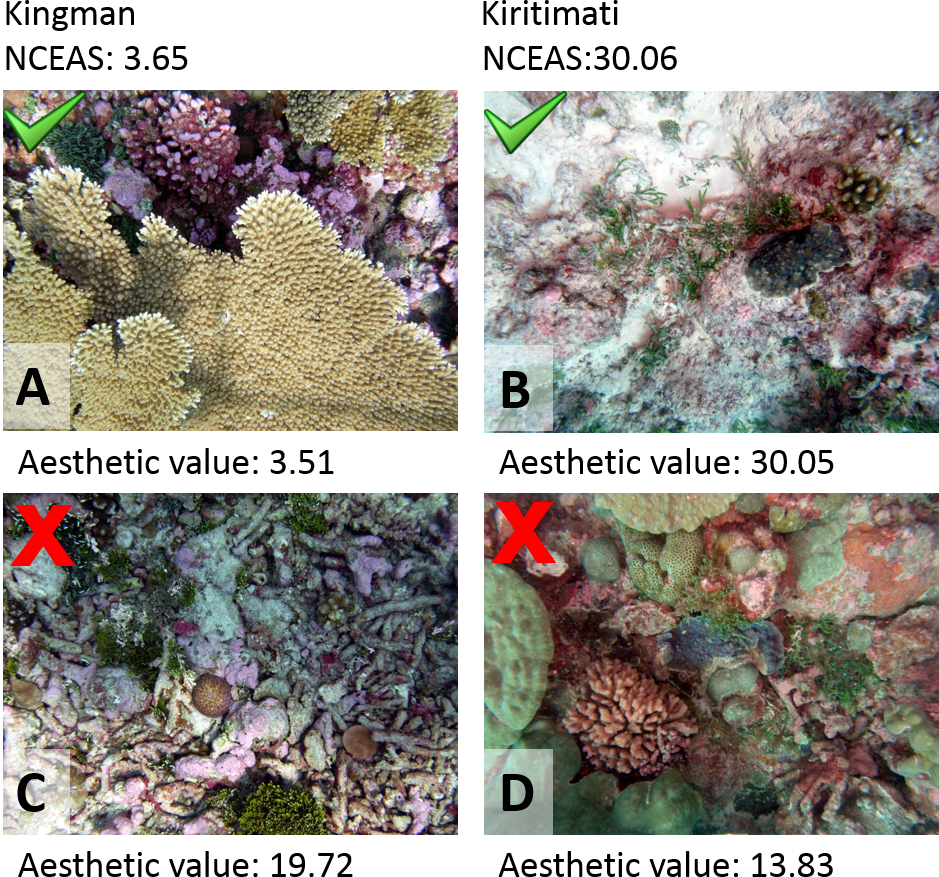
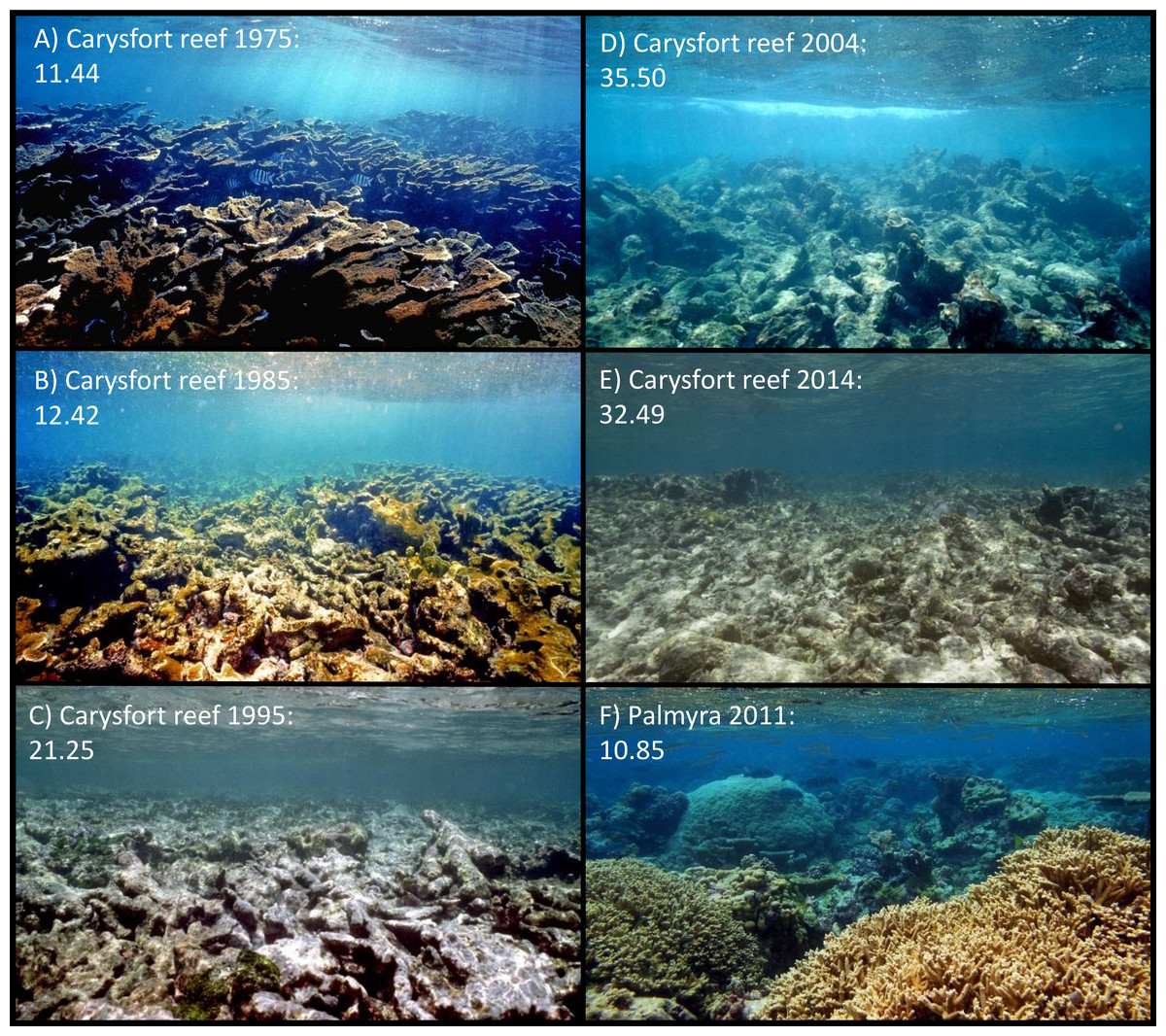
Figure 5: Aesthetic values of Carysfort reef.
(A–E) are taken at the identical location on Carysfort reef, US Caribbean, over a time span of 40 years (photos taken by P Dustan). The aesthetic value calculated for each picture shows a significant degradation of aesthetic appearance during this period. The historic images from 1975 indicate that the aesthetic appearance of this Caribbean reef was comparable to present day pristine reefscapes as for example on Palmyra atoll in the Central Pacific (F, photo taken by J Smith).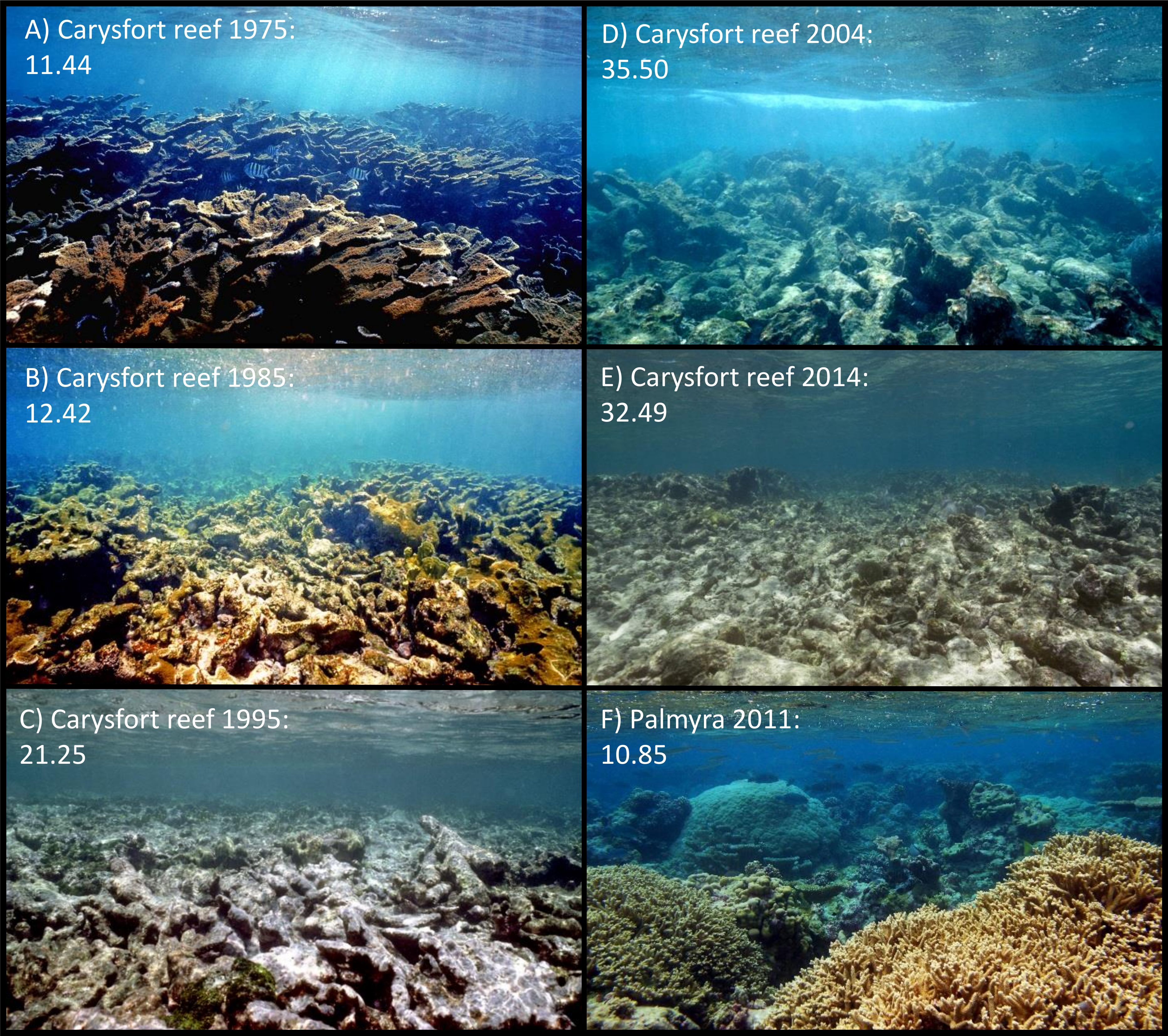
Socioeconomic assessment for stakeholders
This study provides an innovative method to objectively assess parameters associated with a general aesthetic perception of marine environments. Although converting the aesthetic appearance of an entire ecosystem in simple numbers will likely evoke discussions and in some cases resentment, it may provide a powerful tool to disclose effects of implementing conservation measurements on the touristic attractiveness of coastal environments to stakeholders. The approach allows for a rapid analysis of a large number of samples and thus provides a method to cover ecosystems on large scale. Linking aesthetic values to cultural benefits and ultimately revenue for the entire community may be an incentive to further establish and implement protection measurements and could help to evaluate the success and the value to the community of existing conservation efforts. Using monitoring cues that directly address inherent human emotions will more likely motivate and sustain changes in attitude and behavior towards a more sustainable usage of the environmental resources than technical terms and data that carry no local meaning (Carr, 2002; Dinsdale, 2009). Quantifying the aesthetic appearance of these ecosystems targets on one of the most important socioeconomic values of these ecosystems, which are directly tied to culture and the revenue of its local population.
Supplemental Information
Relative importance of features
Relative importance of all 109 features derived from a random forest approach. Features are grouped into three general feature groups, texture of the entire image (texture), color and brightness of the entire image (color), and size, color and brightness, and distribution of objects within the image (objects).
Feature examples
Example pictures of a healthy (left) and a degraded reef (right). The applied measurements for brightness contrast across the whole image f28 shows 97 for (A) and 47 for (B). The green lines depict the central focus region which outlines the segment of interest used for ‘Rule of Third’ features. The orange line marks the Focus region used for features f55 through f56, where an additional margin (μ = 0.1) has been included. (C) and (D) show pictures after segmentation by K means, using K = 2 and m = 1. From these images the number of connected components can be calculated by implementing feature f58 (C = 1,470, D = 2,369). (E) and (G) show the Laplacian image produced for feature f30, (F) and (H) show the resized and normalized Laplacian image which serves as basis for the calculation of f31. The blue bounding boxes contain 81% (E = 0.623, G = 0.611) and 96.04% (F = 0.089, H = 0.079) of the edge energy respectively. (I) and (J) show the images after a three-level wavelet transform performed on the saturation channel IS. K gives an overview of color models used to compare the analyzed images, or objects within images against. The bar chart shows the average NCEAS score where pictures matching to the respective color model were taken. The red boxes indicate the model that fits best to image A and B respectively.
Raw data MATLAB code for feature extraction
Matlab script to extract 109 aesthetic features.
Overview of implemented features
Overview of all 109 implemented features given along their relative importance for the combined coral reef aesthetic value, a short description and the study the respective feature was derived from (1, Datta et al., 2006; 2, Li & Chen, 2009; 3, Ke, Tang & Jing, 2006; 4, this study).
Overview of sampling locations
Overview of sampling locations with coordinates along with their respective NCEAS scores the number of photographic images used from each location and their calculated coral reef aesthetic value. Tukey connecting letters report indicates sites with significant difference in their coral reef aesthetic value.