
Phylogeny and evolution of Lasiopodomys in subfamily Arvivolinae based on mitochondrial genomics
- Published
- Accepted
- Received
- Academic Editor
- Tony Robillard
- Subject Areas
- Biodiversity, Ecology, Genomics, Molecular Biology, Zoology
- Keywords
- Lasiopodomys, Mitochondrial genomes, Phylogenetic analysis, Arvivolinae
- Copyright
- © 2021 Shi et al.
- Licence
- This is an open access article distributed under the terms of the Creative Commons Attribution License, which permits unrestricted use, distribution, reproduction and adaptation in any medium and for any purpose provided that it is properly attributed. For attribution, the original author(s), title, publication source (PeerJ) and either DOI or URL of the article must be cited.
- Cite this article
- 2021. Phylogeny and evolution of Lasiopodomys in subfamily Arvivolinae based on mitochondrial genomics. PeerJ 9:e10850 https://doi.org/10.7717/peerj.10850
Abstract
The species of Lasiopodomys Lataste 1887 with their related genera remains undetermined owing to inconsistent morphological characteristics and molecular phylogeny. To investigate the phylogenetic relationship and speciation among species of the genus Lasiopodomys, we sequenced and annotated the whole mitochondrial genomes of three individual species, namely Lasiopodomys brandtii Radde 1861, L. mandarinus Milne-Edwards 1871, and Neodon (Lasiopodomys) fuscus Büchner 1889. The nucleotide sequences of the circular mitogenomes were identical for each individual species of L. brandtii, L. mandarinus, and N. fuscus. Each species contained 13 protein-coding genes (PCGs), 22 transfer RNAs, and 2 ribosomal RNAs, with mitochondrial genome lengths of 16,557 bp, 16,562 bp, and 16,324 bp, respectively. The mitogenomes and PCGs showed positive AT skew and negative GC skew. Mitogenomic phylogenetic analyses suggested that L. brandtii, L. mandarinus, and L. gregalis Pallas 1779 belong to the genus Lasiopodomys, whereas N. fuscus belongs to the genus Neodon grouped with N. irene. Lasiopodomys showed the closest relationship with Microtus fortis Büchner 1889 and M. kikuchii Kuroda 1920, which are considered as the paraphyletic species of genera Microtus. TMRCA and niche model analysis revealed that Lasiopodomys may have first appeared during the early Pleistocene epoch. Further, L. gregalis separated from others over 1.53 million years ago (Ma) and then diverged into L. brandtii and L. mandarinus 0.76 Ma. The relative contribution of climatic fluctuations to speciation and selection in this group requires further research.
Introduction
Although taxonomical and molecular systematics have led to some progress in the relationship between the genus Lasiopodomys and its related genera, numerous uncertainties remain unelucidated. The species belonging to this genus was first described by Lataste in 1887 as part of the Arvivolinae Gray 1821 (Cricetidae Fischer 1817) subfamily, which includes the genera Phaiomys Blyth 1863, Microtus Schrank 1798, and Neodon Horsfield 1841 (Allen, 1940; Corbet, 1978; Gromov & Polyakov, 1978; Liu et al., 2013; Wang, 2003). The genus Lasiopodomys includes three species from different colonial habitats of life—subterranean (L. mandarinus Milne-Edwards 1871), aboveground (L. brandtii Radde 1861), and plateau (L. fuscus Büchner 1889) by Wilson & Reeder (2005)—with relatively short tail and densely furred plantar surfaces. However, their generic taxonomy is not universally accepted, specifically in relation to Phaiomys, Microtus, and Neodon. Molecular data have revealed that the narrow-headed vole Microtus gregalis Pallas 1779 (formerly included in subgenus Stenocranius Katschenko 1901) is closely related to the species belonging to the genus Lasiopodomys (Abramson & Lissovsky, 2012). Morphological characteristics, such as karyotype (Gladkikh et al., 2016) and mating behavior (Zorenko & Atanasov, 2017), supported its current taxonomic status as L. gregalis. On the other hand, L. fuscus is nested in the genus Neodon Hodgson 1849 clade based on the longer length of ear and tail and greater number of inner angles in M1 and M3 compared with the genus Lasiopodomys (Liu et al., 2012a); moreover, CLOCK, BMA1, and Cytb gene sequences and their complete mitochondrial genomes supported this taxonomical status (Abramson et al., 2009a; Bannikova et al., 2010; Li, Lu & Wang, 2016a; Li et al., 2019; Liu et al., 2017). Recent studies have typically recognized Lasiopodomys as a separate genus that includes the species L. mandarinus and L. brandtii; L. gregalis was not widely accepted, whereas L. fuscus has been transferred to the genus Neodon and named Neodon fuscus.
According to fossils and molecular data, the genus Lasiopodomys originated and speciated during the Pleistocene epoch (∼2.58–0.012 million years ago (Ma)) when quaternary glaciations occurred in this period. Nuclear and mitochondrial phylogenetic estimates have shown that Lasiopodomys originated ∼2.4 Ma, whereas the division between L. gregalis and Lasiopodomys has been estimated to have occurred 1.8 Ma and that between L. mandarinus and L. brandtii was estimated at 0.5–0.95 Ma (Abramson et al., 2009b; Petrova et al., 2015; Li et al., 2017). However, chromosome analysis has shown that karyotype evolution has occurred between L. mandarinus and L. brandtii at ∼2.4 Ma, between Lasiopodomys and L. gregalis at 2.4 Ma, and between other Microtus species at 3 Ma (Gladkikh et al., 2016).
The species in the genus Lasiopodomys inhabit subterranean and aboveground environments and have recently become model species for comparative hypoxia adaptation (Dong et al., 2018; Sun et al., 2018). Species’ adaptation to low oxygen has been reported in numerous studies (Childress & Seibel, 1998; Dong et al., 2018; Nevo, 2013; Witt & Huerta-Sánchez, 2019), and most research has focused on animal models in an artificial environment or has compared them with subterranean rats to reveal the mechanisms of hypoxia (Ashur-Fabian et al., 2004; Malik et al., 2012; Malik et al., 2016). The differences in the environmental adaptability of proximal species are closely related to the historical events experienced during evolution, which play a key role in our understanding of the causes of current differences in life history among these species. However, the historical event that caused the Lasiopodomys species to adapt to a different environment has rarely been mentioned (Dong et al., 2018; Dong, Wang & Jiang, 2020).
Mitochondrial DNA are widely used to study the molecular ecology of animals because it is convenient and economical (Ballard & Rand, 2005; de Freitas et al., 2018; Kenechukwu, Li & An, 2018; Zhang et al., 2018). However, several studies have reported the limitations of mitochondrial DNA use (Galtier et al., 2009), such as recurrent horizontal transfer (Bergthorsson et al., 2003) and adaptive evolution (Bazin, Glémin & Galtier, 2006). The mitochondrial genome is involved in respiratory functions, which are closely associated with oxygen availability (Jain et al., 2016; Santore et al., 2002; Solaini et al., 2010).
In the present study, we sequenced the whole mitochondrial genomes of L. mandarinus, L. brandtii, and N. fuscus, which are species with three repeat individuals, using high-throughput sequencing technology and used the complete mitochondrial genomes of related species from the National Center for Biotechnology Information database to clarify the generic taxonomy of Lasiopodomys and evolutionary history of adaptation on aboveground and subsurface life. The findings of this research provide evolutionary information regarding the hypoxia adaptation of Lasiopodomys.
Materials and Methods
Material preparation and DNA sequencing
Total genomic DNA were extracted from the specimens of L. mandarinus (collected from 34°52′N, 113°85′E; Specimen No. LM023), L. brandtii (collected from 40°53′N, 116°38′E; Specimen No. LB003), and N. fuscus (collected from 34°9′N, 100°2′E; Specimen No. LF010) using the TIANamp Genomic DNA Extraction Kit (TIANGEN, DP304). All specimens were stored at the Animal Museum of Zhengzhou University. The Illumina NovaSeq 6000 (Illumina, San Diego, CA, USA) platform was used for sequencing the samples with a short-insert of 150 bp at ORI-GENE Company, Beijing (https://www.origene.com/).
Genome assembly and annotation
NOVOPlasty 3.6 was used for de novo assembly using the mitochondrial genome of L. mandarinus (GenBank no. JX014233) as a reference (Dierckxsens, Mardulyn & Smits, 2017). All mitochondrial genomes were annotated using GeSeq (Tillich et al., 2017), OGDRAW (Lohse et al., 2013), and GB2sequin (Lehwark & Greiner, 2019) in the MPI-MP CHLOROBOX integrated web tool (https://www.mpimp-golm.mpg.de/chlorobox), which contains the function of the HMMER package for protein-coding genes (PCGs) and ribosomal RNA (rRNA) (Finn, Clements & Edd, 2011), and tRNAscan-SE v2.0.3 for transfer RNAs (tRNAs) (Lowe & Eddy, 1997). Adenine–thymine (AT) skew was calculated as AT skew = (A − T) / (A + T), whereas guanine–cytosine (GC) skew was calculated as GC skew = (G − C)/(G + C). Circular maps were drawn using the CGView Server V 1.0 web tool (http://stothard.afns.ualberta.ca/cgview_server/) for L. mandarinus, L. brandtii, L. gregalis (GenBank no. MN199169), and N. fuscus (Grant & Stothard, 2008).
Molecular phylogenetic analysis and divergence time estimation
Phylogenetic analyses were performed on the whole mitochondrial genome sequences (Appendix S1). Besides the nine mitochondrial genomes that were acquired for the present study, five previously published mitochondrial genomes from L. mandarinus, L. gregalis, and N. fuscus were included; therefore, overall, 37 complete mitochondrial genome sequences from 23 species from the subfamily Arvivolinae were considered for phylogenetic analysis. Moreover, three species from Cricetulus Milne-Edwards 1867 were chosen as the outgroup. All these sequences were aligned using MAFFT v7.450 (Katoh & Standley, 2013). The nucleotide diversity of the PCGs of Lasiopodomys and Arvivolinae was determined using the DNASP v6.12.03 software (Rozas et al., 2017), and the best nucleotide substitution models were constructed using jMODELTEST 2.1.7 and selected using the Akaike information criterion (Darriba et al., 2012).
The phylogenetic relationships of the two different matrices as well as the whole mitochondrial genomes and PCG sequence matrices were constructed using the maximum likelihood (ML) approach in IQ-TREE v1.6.12 (Nguyen et al., 2015) and Bayesian analysis (BI) in the BEAST v1.8.4 program (Drummond & Rambaut, 2007). We conducted analysis using 5000 ultrafast bootstrap replicates and the best-fit model in the IQ-TREE software. To determine the maximum clade credibility trees of two different matrices, BEAST analyses were performed using the GTR+G+I substitution models identified above and the uncorrelated relaxed clocks for clock type (Drummond et al., 2006), Yule process for tree prior (Gernhard, 2008), and other default parameters. Each Markov chain Monte Carlo of 20,000,000 generations was sampled in every 10,000 generations. The effective sample sizes were estimated using Tracer v1.7 for all parameters more than 200 (Rambaut et al., 2018). Maximum clade credibility trees were constructed using TreeAnnotator v1.8.4 with a burn-in of the first 20% of the sampled trees (Drummond & Rambaut, 2007). Positive selection in all 13 PCGs was determined using branch models and branch-site models via phylogenetic analysis using ML (PAML4.7) programs (Yang, 2007). Branch models were used with the one-ratio model, i.e., all the species had the same ω ratio, and the ω = 1 model, with all species in natural selection. Based on the phylogenetic tree, we estimated the ω values of each PCG. The branch-site models used all Lasiopodomys species as the foreground branches, and the likelihood ratio test (LRT) was conducted to assess the statistical significance of positive selection.
The molecular divergence time was estimated using the Yule and birth–death processes for trees before implementing phylogeny construction using BEAST v1.8.4 (Gernhard, 2008; Heath, Huelsenbeck & Stadler, 2014). Marginal likelihood estimation for path sampling and stepping-stone sampling (Xie et al., 2011) using 5,000,000 in chain lengths of 500 path steps was used to sample the likelihood of every 5,000 chains (Baele et al., 2012; Baele et al., 2013). We applied three constraints to calibrate the tree at three prior nodes: (1) the divergence time of the Taiwan vole, Microtus kikuchii Kuroda 1920, and the reed vole Microtus fortis, of which the split between the subgenus Alexandromys Ognev 1914 and Pallasiimus Schrank 1798 was estimated via molecular clock analysis at ∼1.19 ± 0.19 Ma (Bannikova et al., 2010; Gao et al., 2017), (2) the earliest known fossil of Eothenomys Allen 1924 at 2.0 Ma (Liu et al., 2012a; Kohli et al., 2014), and (3) the oldest fossil of Arvicola, which was estimated at 3.0–3.5 Ma (Abramson et al., 2009a; Chen et al., 2012); we used the mean value of 3.25 Ma.
Ecological niche modeling
The maximum entropy (Maxent) method was used to predict the current potential geographic distributions of L. mandarinus, L. brandtii, L. gregalis, and N. fuscus as well as their suitable distributions during the mid-Holocene, 6,000 years ago (kya), Last Glacial Maximum (LGM; 22 kya), and Last Interglacial (LIG; 120–140 kya) epochs (Phillips, Anderson & Schapire, 2006; Elith et al., 2011). Presence records were obtained for all four species according to the GBIF database and published papers (Appendix S2). Climatic variables with 19 bioclimatic layers were obtained from the database WorldClim version 1.4 at a resolution of 2.5 arc-minute grid format (Hijmans et al., 2005). The potential distributions of the species during the LGM and Holocene periods were predicted using both MIROC-ESM and CCSM4 models (Watanabe et al., 2011; Shields et al., 2012). Strongly correlated bioclimatic layers (r > 0.9) as determined using Pearson’s correlation analysis in R 3.6.2 (Appendix S3) (R Development Core Team, 2013) were excluded. Moreover, Maxent was independently performed among these species using area under the receiver operating characteristic curve (AUC) prediction model evaluation (DeLong, DeLong & Clarke-Pearson, 1988; Fawcett, 2006).
Results
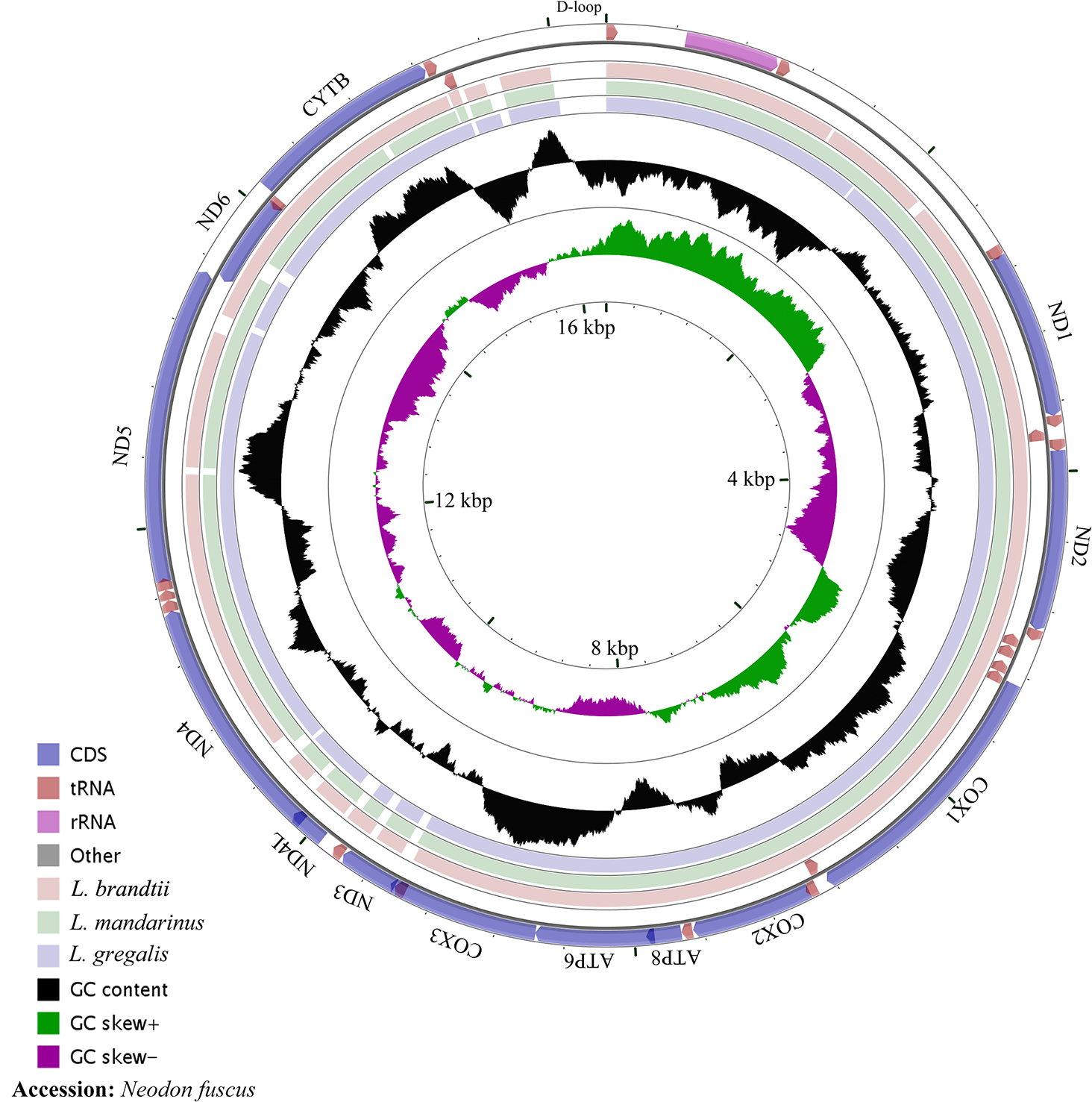
The whole mitochondrial genome length of L. mandarinus was 16,562 bp, with the same sequences among repeated individuals. The mitochondrial genome length of L. brandtii was only 5 bp shorter than that of L. mandarinus, whereas that of N. fuscus was 220 bp shorter than that of L. mandarinus (Fig. 1). On the other hand, L. mandarinus was found to be 234 bp longer than the former sequenced mitogenomes (GenBank no. KF819832& JX014233). All sequences of the three species were longer than those of L. gregalis, a species previously in the genus Microtus, with sequence lengths of 16,292 bp (GenBank no. MN199169) and 16,294 bp (GenBank no. MN199170). All the three mitogenomes were assembled into a typical circular map with 13 PCGs, 22 tRNAs, 2 rRNAs (rrn12 and rrn16), and a D-loop region (Fig. 1, Table 1). Five types of start codons—ATA, ATC, ATG, ATT, and GTG—were identified among the PCGs, whereas three types of stop codons were identified for these species.
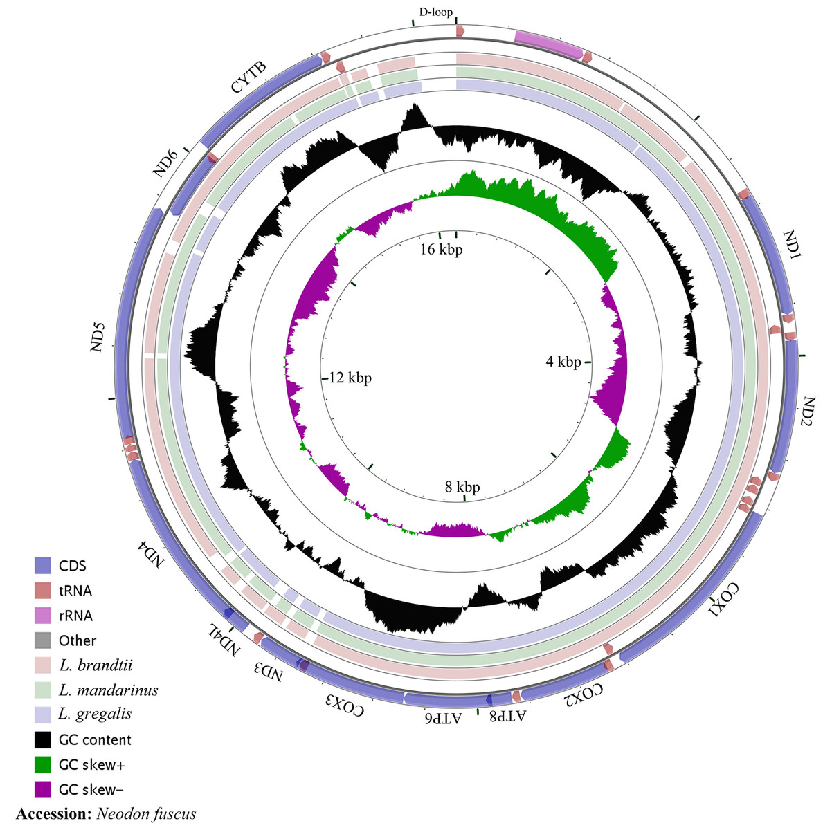
Figure 1: The complete mitochondrial genome map and GC skew of Neodon fuscus, Lasiopodomys brandtii, L. mandarinus, and L. gregalis.
| Genes | Position (bp) | Strat/stop codon | ||||||
|---|---|---|---|---|---|---|---|---|
| L. brabdtii | L. mandarinus | L. gregalis | Neodon fuscus | L. brabdtii | L. mandarinus | L. gregalis | Neodon fuscus | |
| trnF-GAA | 1-66 | 1-66 | 1-66 | 1-66 | ||||
| rrn12 | 69–1017 | 69–1018 | 69–1017 | 69–1015 | ||||
| trnV-UAC | 1019–1087 | 1019–1088 | 1018–1087 | 1016–1086 | ||||
| rrn16 | 1088–2641 | 1089–2652 | 1088–2649 | 1087–2648 | ||||
| trnL-UAA | 2650–2724 | 2655–2729 | 2651–2725 | 2650–2724 | ||||
| ND1 | 2710–3681 | 2715–3686 | 2726–3680 | 2725–3679 | GTG/TAG | GTG/TAG | GTG/TAG | GTG/TAG |
| trnI-GAU | 3680–3748 | 3685–3752 | 3681–3748 | 3680–3747 | ||||
| trnQ-UUG | 3746–3817 | 3750–3821 | 3746–3817 | 3745–3816 | ||||
| trnM-CAU | 3820–3888 | 3823–3891 | 3820–3888 | 3818–3886 | ||||
| ND2 | 3889–4923 | 3865–4926 | 3889–4923 | 3887–4921 | ATC/TAA | ATC/TAA | ATT/TAA | ATC/TAA |
| trnW-UCA | 4925–4991 | 4928–4994 | 4925–4991 | 4923–4989 | ||||
| trnA-UGC | 4993–5061 | 4996–5064 | 4993–5061 | 4991–5059 | ||||
| trnN-GUU | 5064–5133 | 5067–5136 | 5064–5133 | 5062–5131 | ||||
| trnC-GCA | 5168–5235 | 5171–5237 | 5167–5234 | 5163–5230 | ||||
| trnY-GUA | 5236–5302 | 5238–5303 | 5235–5301 | 5231–5297 | ||||
| COX1 | 5268–6848 | 5296–6849 | 5303–6847 | 5299–6843 | ATG/TAA | ATG/TAA | ATG/TAA | ATG/TAA |
| trnS-UGA | 6846–6914 | 6847–6915 | 6845–6913 | 6841–6909 | ||||
| trnD-GUC | 6918–6985 | 6919–6986 | 6918–6985 | 6913–6980 | ||||
| COX2 | 6978–7670 | 6979–7671 | 6987–7670 | 6982–7665 | ATG/TAA | ATG/TAA | ATA/TAG | ATG/TAA |
| trnK-UUU | 7674–7737 | 7675–7738 | 7674–7738 | 7669–7732 | ||||
| ATP8 | 7738–7941 | 7739–7942 | 7739–7942 | 7733–7936 | ATG/TAA | ATG/TAA | ATG/TAA | ATG/TAA |
| ATP6 | 7899–8579 | 7900–8580 | 7900–8580 | 7894–8574 | ATG/TAA | ATG/TAA | ATG/TAA | ATG/TAA |
| COX3 | 8474–9412 | 8508–9413 | 8580–9363 | 8574–9357 | ATG/TAG | ATG/TAG | ATG/TAG | ATG/TAG |
| trnG-UCC | 9363–9430 | 9364–9431 | 9364–9431 | 9358–9426 | ||||
| ND3 | 9431–9778 | 9432–9779 | 9432–9779 | 9427–9774 | ATT/TAA | ATT/TAA | ATT/TAA | GTG/TAA |
| trnR-UCG | 9780–9846 | 9781–9847 | 9781–9847 | 9776–9842 | ||||
| ND4L | 9849–10145 | 9851–10147 | 9850–10146 | 9844–10140 | ATG/TAA | ATG/TAA | ATG/TAA | ATG/TAA |
| ND4 | 9962–11521 | 10141–11523 | 10140–11517 | 10134–11511 | ATG/TTA | ATG/TTA | ATG/TTA | ATG/TTA |
| trnH-GUG | 11517–11583 | 11519–11584 | 11518–11585 | 11512–11579 | ||||
| trnS-UCU | 11584–11642 | 11585–11643 | 11586–11644 | 11580–11638 | ||||
| trnL-UAG | 11642–11711 | 11643–11712 | 11644–11713 | 11638–11707 | ||||
| ND5 | 11691–13523 | 11692–13524 | 11714–13525 | 11708–13519 | ATT/TAA | ATT/TAA | ATA/TAA | ATA/TAA |
| ND6 | 13520–14104 | 13521–14147 | 13522–14046 | 13516–14040 | ATG/TTA | ATG/TTA | ATG/TTA | ATG/TTA |
| trnE-UUC | 14042–14110 | 14046–14114 | 14047–14115 | 14041–14109 | ||||
| Cytb | 14113–15258 | 14117–15262 | 14121–15263 | 14115–15257 | ATG/TAA | ATG/TAA | ATG/TAA | ATG/TAA |
| trnT-UGU | 15260–15326 | 15265–15331 | 15265–15331 | 15260–15327 | ||||
| trnP-UGG | 15566–15633 | 15522–15589 | 15332–15399 | 15328–15395 | ||||
The nucleotide composition of L. brandtii, L. mandarinus, and N. fuscus was biased for A+T by 59.5%, 59.5%, and 58.4%, respectively. All these mitogenomes showed a positive AT skew of 0.08 for L. brandtii, 0.09 for L. mandarinus, and 0.09 for N. fuscus. However, these species showed a negative GC skew ranging from −0.30 for L. brandtii to −0.34 for L. mandarinus (Fig. 1, Table 2). L. gregalis showed higher AT skew (0.10) and GC skew (−0.30) compared with the other three species. Among the 13 PCGs in these 4 species, nucleotide composition ranged from −0.69 in ATP8 to −0.16 in ND4L for L. mandarinus, with a GC skew ranging from −0.14 in ND4L for L. brandtii to 0.33 in ND6 for L. mandarinus. Similarly, all 13 PCGs exhibited a negative GC skew; however, COX1, ND4L in all species, COX3 in L. brandtii and L. mandarinus, and ND3 in N. fuscus showed a negative AT skew and ND3 in L. brandtii and L. mandarinus had an AT skew of 0 (Table 2).
| Species | contents | T | C | A | G | GC skew | AT skew |
|---|---|---|---|---|---|---|---|
| L. brabdtii | whole | 27.4 | 26.4 | 32.1 | 14.1 | −0.30 | 0.08 |
| ATP6 | 28.3 | 29.8 | 31 | 10.9 | −0.46 | 0.05 | |
| ATP8 | 26 | 27 | 37.7 | 9.3 | −0.49 | 0.18 | |
| COX1 | 29.5 | 25.5 | 27.1 | 18 | −0.17 | −0.04 | |
| COX2 | 26.3 | 27.7 | 31.6 | 14.4 | −0.32 | 0.09 | |
| COX3 | 29.3 | 26.8 | 28.6 | 15.4 | −0.27 | −0.01 | |
| cytB | 27 | 29.1 | 30.5 | 13.4 | −0.37 | 0.06 | |
| ND1 | 28.5 | 28.9 | 30.7 | 11.9 | −0.42 | 0.04 | |
| ND2 | 26.7 | 31 | 33.9 | 8.4 | −0.57 | 0.12 | |
| ND3 | 30.7 | 26.1 | 30.5 | 12.6 | −0.35 | 0.00 | |
| ND4 | 27.8 | 28.3 | 31 | 12.9 | −0.37 | 0.05 | |
| ND4L | 31.3 | 30.3 | 23.6 | 14.8 | −0.34 | −0.14 | |
| ND5 | 28 | 27.8 | 32.4 | 11.8 | −0.40 | 0.07 | |
| ND6 | 20.6 | 30.9 | 38.6 | 9.9 | −0.51 | 0.30 | |
| L. gregalis | whole | 26.5 | 27.2 | 32.1 | 14.2 | −0.31 | 0.10 |
| ATP6 | 17.6 | 30.5 | 29.8 | 12 | −0.44 | 0.26 | |
| ATP8 | 24.5 | 29.4 | 38.7 | 7.4 | −0.60 | 0.22 | |
| COX1 | 28.7 | 26.5 | 26.9 | 18 | −0.19 | −0.03 | |
| COX2 | 28.3 | 26.1 | 30 | 15.6 | −0.25 | 0.03 | |
| COX3 | 27.6 | 28.4 | 29.1 | 14.9 | −0.31 | 0.03 | |
| cytB | 26.5 | 29.7 | 30.3 | 13.5 | −0.38 | 0.07 | |
| ND1 | 25.9 | 31.5 | 30 | 12.6 | −0.43 | 0.07 | |
| ND2 | 26.1 | 29.7 | 35 | 9.3 | −0.52 | 0.15 | |
| ND3 | 27.3 | 29.9 | 30.7 | 12.1 | −0.42 | 0.06 | |
| ND4 | 27.1 | 29.4 | 31.9 | 11.4 | −0.44 | 0.08 | |
| ND4L | 30.6 | 31.3 | 26.6 | 11.4 | −0.47 | −0.07 | |
| ND5 | 25.9 | 30.4 | 31.5 | 12.3 | −0.42 | 0.10 | |
| ND6 | 22.4 | 29.4 | 39.6 | 8.7 | −0.54 | 0.28 | |
| L. mandarinus | whole | 27.1 | 27.1 | 32.4 | 13.4 | −0.34 | 0.09 |
| ATP6 | 29.8 | 29.2 | 30.7 | 10.3 | −0.48 | 0.01 | |
| ATP8 | 27.9 | 28.9 | 37.7 | 5.4 | −0.69 | 0.15 | |
| COX1 | 28.7 | 26.5 | 27.7 | 17.1 | −0.22 | −0.02 | |
| COX2 | 27 | 27.1 | 32.5 | 13.4 | −0.34 | 0.09 | |
| COX3 | 29 | 28.4 | 28 | 14.6 | −0.32 | −0.02 | |
| cytB | 26.5 | 30.7 | 30.6 | 12.1 | −0.43 | 0.07 | |
| ND1 | 28.4 | 29.1 | 30.2 | 12.2 | −0.41 | 0.03 | |
| ND2 | 26.9 | 30.9 | 33.9 | 8.3 | −0.58 | 0.12 | |
| ND3 | 32.2 | 24.1 | 32.2 | 11.5 | −0.35 | 0.00 | |
| ND4 | 28 | 28.5 | 32.3 | 11.2 | −0.44 | 0.07 | |
| ND4L | 32 | 29.3 | 26.6 | 21.1 | −0.16 | −0.09 | |
| ND5 | 27 | 28.9 | 33 | 11.2 | −0.44 | 0.10 | |
| ND6 | 20 | 30.7 | 40.1 | 9.2 | −0.54 | 0.33 | |
| Neodon fuscus | whole | 26.5 | 27.2 | 31.9 | 14.4 | −0.31 | 0.09 |
| ATP6 | 27.6 | 31.3 | 28.8 | 12.3 | −0.44 | 0.02 | |
| ATP8 | 27 | 27 | 37.7 | 8.3 | −0.53 | 0.17 | |
| COX1 | 29 | 26.4 | 26.6 | 18 | −0.19 | −0.04 | |
| COX2 | 26.8 | 26.8 | 31.5 | 14.9 | −0.29 | 0.08 | |
| COX3 | 27.1 | 29.5 | 28 | 15.4 | −0.31 | 0.02 | |
| cytB | 25.8 | 31.3 | 28.8 | 14 | −0.38 | 0.05 | |
| ND1 | 25.9 | 30.7 | 31 | 12.4 | −0.42 | 0.09 | |
| ND2 | 25.7 | 30.7 | 35 | 8.6 | −0.56 | 0.15 | |
| ND3 | 29.6 | 28.2 | 28.2 | 14.1 | −0.33 | −0.02 | |
| ND4 | 27 | 29.1 | 31 | 12.9 | −0.39 | 0.07 | |
| ND4L | 29.2 | 30.2 | 26.8 | 13.8 | −0.37 | −0.04 | |
| ND5 | 26.2 | 29.8 | 31.5 | 12.5 | −0.41 | 0.09 | |
| ND6 | 21.8 | 28.8 | 39.9 | 9.4 | −0.51 | 0.29 |
The nucleotide diversity among the published Arvicolinae mitogenome sequences and our study species was 0.1429 ± 0.0001, whereas the nucleotide diversity of the mitogenomes of Lasiopodomys was 0.0836 ± 0.0155 (Fig. 2). The total nucleotide diversity in all 13 PCGs of Arvicolinae and the genus Lasiopodomys was 0.1603 ± 0.0027 and 0.0953 ± 0.0180, respectively (Fig. 2). In Arvicolinae, nucleotide diversity ranged from 0.1378 ± 0.0049 in Cytb to 0.1977 ± 0.0077 in ND3, whereas for Lasiopodomys, it ranged from 0.0829 ± 0.0157 in COX3 to 0.1256 ± 0.021 in ND4L.
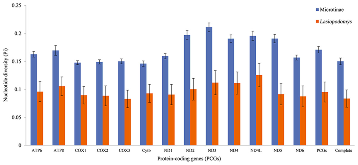
Figure 2: Nucleotide diversity of each protein-coding gene (PCG), concatenate PCG, and whole mitochondrial genomes of Microtinae (blue) and Lasiopodomys (orange).

Figure 3: Divergence time for Lasiopodomys with whole mitochondrial genomes. The numbers on each node are posterior probabilities and bootstrap values.
Blue bars show 95% highest posterior density intervals of node heights. Three red circles were fossil time. The genus of Cricetulus was used as an outgroup.
The results of the ML and Bayesian approaches were applied to the datasets of the whole mitogenomes, and the 13 PCG matrices inferred the same topology of the phylogenetic tree structure (Fig. 3). Our results supported that Lasiopodomys, Microtus, and Neodon have close relationships with the basal group of Proedromys Thomas 1911. Furthermore, the phylogenetic tree suggested that L. brandtii, L. mandarinus, and L. gregalis formed the genus of Lasiopodomys, whereas N. fuscus showed a close relationship with N. irene, belonging to the genus Neodon. Microtus was subdivided into two groups: one containing M. fortis and M. kikuchii, which were strongly supported as the sister group to Lasiopodomys, and the other was the basal group of the above species.
In the branch models, the one-ratio model was determined as superior to the ω = 1 model (df = 1, p < 0.01), suggesting that all the PCGs in the mitogenomes of Lasiopodomys undergo purifying selection (Table 3). In the branch-site model, only the ATP6 gene was present in some positive selection sites (60I 0.987, p < 0.01) in Lasiopodomys (Table 3). Moreover, positive selection sites were predicted in Cox1, Cox3, Cytb, ND2, ND3, and ND5. However, the LRTs were not significant.
The species divergence time among the Lasiopodomys species and related genera was calculated using the uncorrelated relaxed molecular clock model, which was calibrated with three prior divergence times of Arvicolinae (Fig. 3). The results suggested that the origin of Lasiopodomys was no earlier than the early Pleistocene epoch (∼0.781–2.58 Ma), with a possible most common ancestor of Lasiopodomys at ∼1.79 Ma (95% HPD values: ∼1.52–2.09 Ma). The split between L. brandtii and L. mandarinus was dated to the early Pleistocene period at ∼0.76 Ma (95% HPD values: ∼0.58–0.98 Ma), whereas the separation of both from L. gregalis was dated to the early Pleistocene epoch at 1.53 Ma (95% HPD values: ∼1.26–1.81 Ma). The estimated divergence event of N. fuscus and N. irene was found to be during the early Pleistocene epoch at 1.44 Ma (95% HPD Interval: ∼1.12–1.75 Ma).
The high AUC values determined via ecological niche modeling (ENM) indicated the good performance of the model predictions of this study (Appendix S4). During the periods from the LIG to present, all species of Lasiopodomys showed no evident loss of a suitable habitat. A western expansion of L. brandtii has been predicted in Northeast China, Inner Mongolia, and South Siberia, whereas a weak fragment was predicted for L. gregalis among the Eurasia regions (Fig. 4). Moreover, suitable areas were predicted in highly suitable habitat regions during the LGM in these species. More northern suitable areas were predicted during the LIG, and a northern expansion was predicted during the transition from the Holocene period to the present (Fig. 4). In addition, highly suitable habitats were observed for N. fuscus in the Hengduan Mountains during all periods, whereas more eastern distributions were predicted during the LGM (Fig. 4).
| Gene | Model | lnL | Models compared | Parameter Estimates | LRT ( P-value) | |
|---|---|---|---|---|---|---|
| ATP6 | Branch-model | A:One-ratio | −6321.793406 | ω= 0.02625 | p < 0.01 | |
| B:Omega = 1 | −7802.578602 | B vs A | ω=1 | |||
| Branch-site model | Null | −6298.662308 | null vs A | 7 A 0.578 | P<0.01 | |
| Model A | −6295.340396 | 60 I 0.987* | ||||
| ATP8 | Branch-model | A:One-ratio | −2156.664937 | ω=0.16120 | p < 0.01 | |
| B:Omega = 1 | −2304.668614 | B vs A | ω=1 | |||
| Branch-site model | Null | −2092.811906 | 1 | |||
| Model A | −2092.811906 | null vs A | NA | |||
| Cox1 | Branch-model | A:One-ratio | −12806.04872 | B vs A | ω=0.00534 | p < 0.01 |
| B:Omega = 1 | −17316.74494 | ω=1 | ||||
| Branch-site model | Null | −12712.24034 | null vs A | 57 I 0.779 | 0.077 | |
| Model A | −12710.67689 | 487 T 0.965* | ||||
| Cox2 | Branch-model | A:One-ratio | −5779.531238 | ω=0.01386 | p < 0.01 | |
| B:Omega = 1 | −7512.338542 | B vs A | ω=1 | |||
| Branch-site model | Null | −5711.411586 | 1 | |||
| Model A | −5711.411586 | null vs A | NA | |||
| Cox3 | Branch-model | A:One-ratio | −6864.103188 | ω=0.01989 | p < 0.01 | |
| B:Omega = 1 | −8741.926003 | B vs A | ω=1 | |||
| Branch-site model | Null | −6757.123306 | ||||
| Model A | −6757.116417 | null vs A | 50 N 0.642 | 0.9065 | ||
| 62 V 0.517 | ||||||
| 203 F 0.593 | ||||||
| Cytb | Branch-model | A:One-ratio | −10097.89327 | ω=0.02761 | ||
| B:Omega = 1 | −12504.74705 | B vs A | ω=1 | p < 0.01 | ||
| Branch-site model | Null | −10010.08824 | ||||
| Model A | −10009.07827 | null vs A | 4 M 0.976* | 0.1552 | ||
| 7 K 0.892 | ||||||
| 116 I 0.567 | ||||||
| 242 V 0.522 | ||||||
| 315 I 0.516 | ||||||
| ND1 | Branch-model | A:One-ratio | −9200.160474 | ω=0.02426 | ||
| B:Omega = 1 | −11391.13236 | B vs A | ω=1 | p < 0.01 | ||
| Branch-site model | Null | −9015.80101 | ||||
| Model A | −9015.745075 | null vs A | NA | 0.738 | ||
| ND2 | Branch-model | A:One-ratio | −11468.97809 | ω=0.06165 | ||
| B:Omega = 1 | −13190.51757 | B vs A | ω=1 | p < 0.01 | ||
| Branch-site model | Null | −11268.21175 | ||||
| Model A | −11268.21175 | null vs A | 11 F 0.747 | 1 | ||
| 14 F 0.816 | ||||||
| 31 I 0.845 | ||||||
| 95 T 0.837 | ||||||
| 122 I 0.856 | ||||||
| 207 I 0.845 | ||||||
| 220 H 0.867 | ||||||
| 228 K 0.847 | ||||||
| 235 N 0.860 | ||||||
| 241 L 0.858 | ||||||
| ND3 | Branch-model | A:One-ratio | −4086.367921 | ω=0.06686 | ||
| B:Omega = 1 | −4686.550566 | B vs A | ω=1 | p < 0.01 | ||
| Branch-site model | Null | −3969.046821 | ||||
| Model A | −3969.013478 | null vs A | 6 A 0.811 | 0.7962 | ||
| 14 S 0.790 | ||||||
| 20 V 0.861 | ||||||
| 108 Q 0.849 | ||||||
| ND4 | Branch-model | A:One-ratio | −15050.32692 | ω=0.04173 | ||
| B:Omega = 1 | −17886.34941 | B vs A | ω=1 | p < 0.01 | ||
| Branch-site model | Null | −14856.89331 | ||||
| Model A | −14856.89325 | null vs A | NA | 0.992 | ||
| ND4L | Branch-model | A:One-ratio | −3210.084127 | ω=0.05007 | ||
| B:Omega = 1 | −3775.223753 | B vs A | ω=1 | p < 0.01 | ||
| Branch-site model | Null | −3151.8857 | ||||
| Model A | −3151.8857 | null vs A | NA | 1 | ||
| ND5 | Branch-model | A:One-ratio | −19894.46685 | ω=0.04666 | ||
| B:Omega = 1 | −23436.47839 | B vs A | ω=1 | p < 0.01 | ||
| Branch-site model | Null | −19737.31375 | ||||
| Model A | −19737.31225 | null vs A | 194 E 0.512 | 0.9563 | ||
| 575 K 0.969* | ||||||
| ND6 | Branch-model | A:One-ratio | −5081.893461 | ω=0.06927 | ||
| B:Omega = 1 | −5814.462234 | B vs A | ω=1 | p < 0.01 | ||
| Branch-site model | Null | −4971.821282 | ||||
| Model A | −4971.821283 | null vs A | NA | 1 | ||
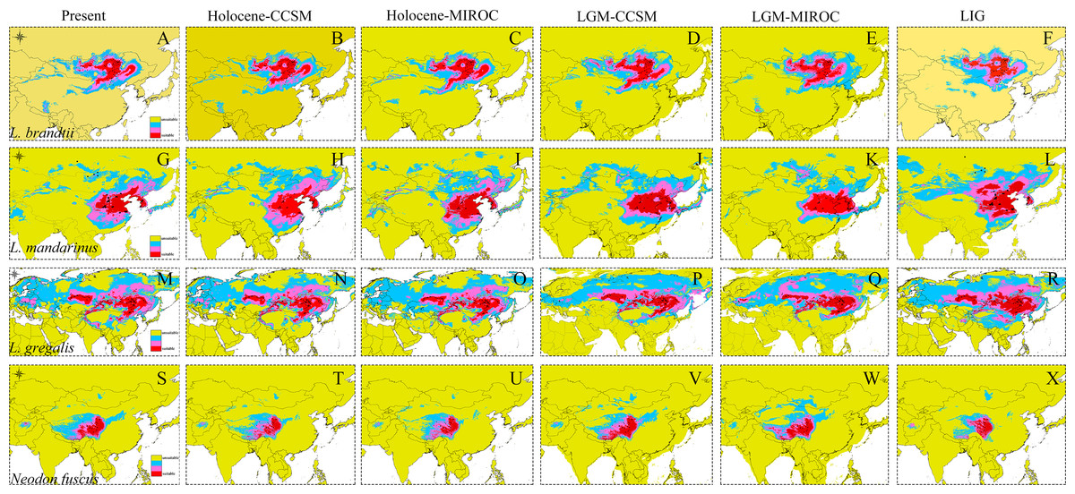
Figure 4: Ecological niche modeling of Lasiopodomys and Neodon.
Lasiopodomys brandtii (A–F), L. mandarinus (G–L), L. gregalis (M–R), and Neodon fuscus (S–X) under the current climate and three periods in the past: the mid-Holocene, the Last Glacial Maximum (LGM), and the Last Interglacial Maxima (LIG).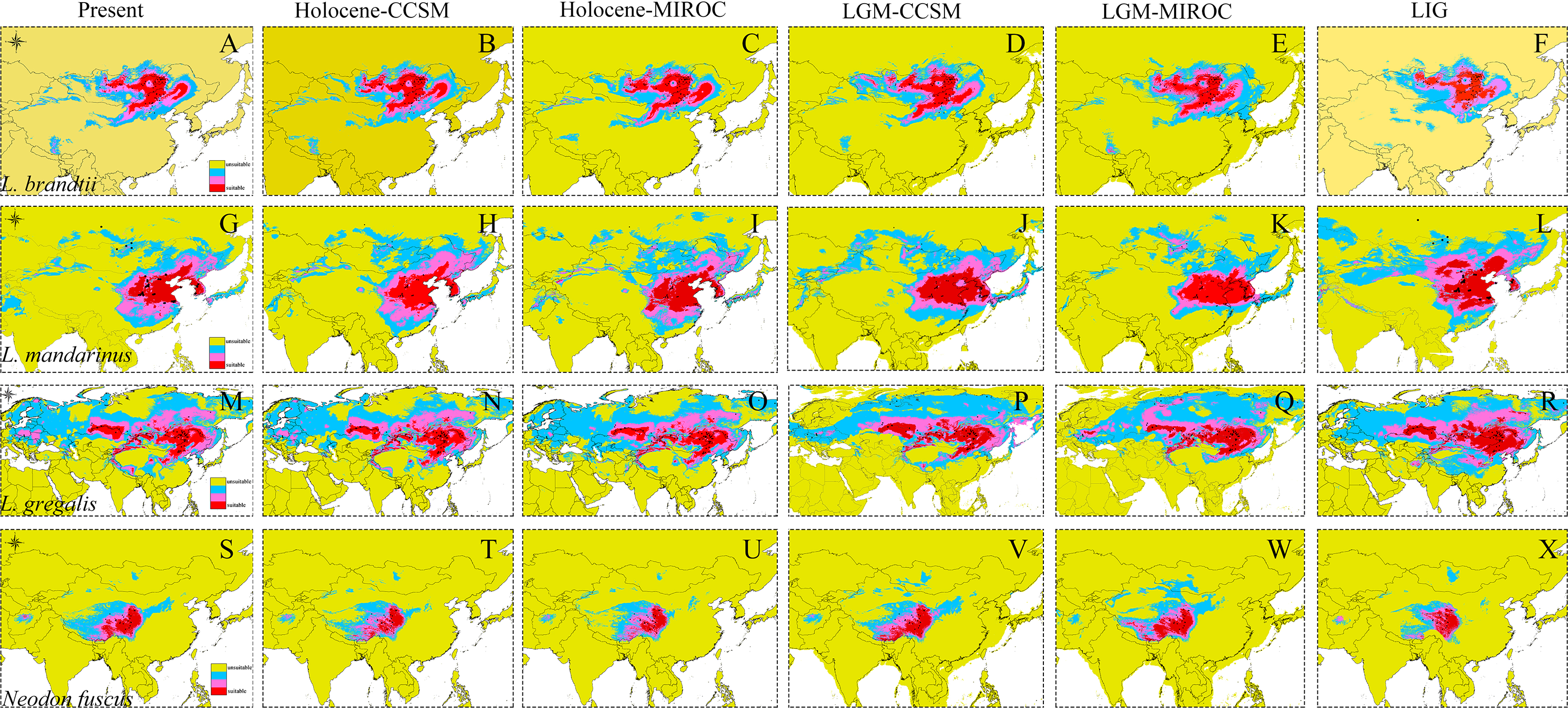
Discussion
Structural features of the whole mitochondrial genome of Lasiopodomys
Among the nine complete mitochondrial sequences, all the species showed same sequences in the three repeated individuals, thereby supporting the accuracy and low intraspecific variation of our studies (Brown & Simpson, 1981). Although N. fuscus showed similar characteristics to previously sequenced mitogenomes (GenBank no. MG833880), L. mandarinus exhibited a longer sequence than that previously reported (Cong et al., 2016; Li, Lu & Wang, 2016a; Li et al., 2016b; Li et al., 2019). This difference may be due to nucleotide errors, particularly in tandem repeats, caused by different sequencing technologies: Sanger sequencing versus high-throughput sequencing (Pfeiffer et al., 2018). All these differences occurred in the intergenic region, with little impact on subsequent analysis. Therefore, we reserved both types of sequence data in the subsequent analysis.
All the PCGs of these species, similar to the other Arvicolinae mitogenomes, had an incomplete stop codon that was automatically filled during the transcription process in the mitogenomes of animals, with no effect on translation (Ojala, Montoya & Attardi, 1981). Similar to previous studies, the nucleotide diversity of all the PCGs in both Lasiopodomys and Arvicolinae typically showed the highest divergence in the NADH dehydrogenase complex and the lowest divergence in the cytochrome c oxidase subunit complex and cytochrome B gene (Huang et al., 2019; Ramos et al., 2018). The nucleotide sequence diversity of the NADH dehydrogenase gene groups may be affected by variations in the historical environment (Ramos et al., 2018; Mueller, 2006). Similar to previously published mitogenomes, the AT skew of Lasiopodomys and N. fuscus was consistent with that of vertebrates (Zhang, Cheng & Ge, 2019; Martin, 1995), further indicating evolutionary pressure related to the mechanism of DNA replication (Charneski et al., 2011; Dai & Holland, 2019).
Phylogenetic relationships of Lasiopodomys
Our molecular phylogenetic analysis results were highly consistent those of previous studies. In our study, the subfamily Arvicolinae was supported as a monophyletic group based on the molecular data of Cytb, COX1, GHR, CLOCK, and BMAL1 (Abramson et al., 2009b; Buzan et al., 2008; Liu et al., 2017; Martin et al., 2000; Sun et al., 2018). Our results suggest that N. (Lasiopodomys) fuscus within the genus Neodon forms a sister relationship with N. irene, consistent with the results reported by Chen et al. (2012) and Li et al. (2019). The stable clustering of L. brandtii, L. mandarinus, and L. gregalis into one group confirms the systematic positions of Lasiopodomys. This topology was consistent with that of other phylogenetic studies based on nuclear genes (Sun et al., 2018), mitochondrial DNA (Abramson et al., 2009a; Liu et al., 2012b; Martínková & Moravec, 2012; Petrova et al., 2016), and whole genomes (Li, Lu & Wang, 2016a; Li et al., 2019; Tian et al., 2020). However, it contradicts with the systematic position based on the morphological characteristics of these species (Allen, 1940; Corbet, 1978; Wilson & Reeder , 2005). Further, L. brandtii and L. mandarinus have consistently presented as a sister group in molecular phylogenetic studies, with seldom distinguished morphological characteristics but different aboveground and underground habitats, suggesting a mechanism of environmental adaptation during rapid speciation (Alexeeva, Erbajeva & Khenzykhenova, 2015; Dong et al., 2018; Li et al., 2017). Other species of Microtus and Neodon were not found in the monophyletic group (Liu et al., 2012a); M. kikuchii and M. fortis were grouped as sister lineages within the Lasiopodomys clades and were considered belonging to the subgenus Alexandromys based on phylogenetic research (Mezhzherin, Zykov & Morozov-Leonov, 1993), allozymes, and Cytb (Bannikova et al., 2010). All these genera form a “Microtus s. l.,” which could be the “core Arvicolinae” (Baca et al., 2019).
Evolution and demographic history of Lasiopodomys
When inferring the divergence time of Lasiopodomys and related genera, both the Yule process and birth–death process speciation models were required with multiple fossil calibration nodes employed in phylogenetic analysis to develop more robust estimates (Drummond & Rambaut, 2007; Humphreys et al., 2016). Based on complete genomes and PCG phylogenetic trees, both models presented similar estimates of a relatively recent origin and divergence time for Microtus s. l. during the early Pleistocene epoch. The oldest reported fossil of Microtus s. l. was during the early Pleistocene epoch (Chaline et al., 1999). An arid and cold environment raised species dispersal and speciation in response to Pleistocene climatic fluctuations (Vasconcellos et al., 2019). Our study supported the first appearance of Lasiopodomys in the late early Pleistocene epoch from the Transbaikal area (Alexeeva, Erbajeva & Khenzykhenova, 2015; Li et al., 2017) at ∼1.52–2.09 Ma (Petrova et al., 2016) but later than that estimated by chromosomes at 3 Ma (Gladkikh et al., 2016). At ∼1.28–1.81 Ma, the morphological characters of L. gregalis proposed the earliest clades of modern Lasiopodomys, as indicated by molecular data and fossils (Abramson et al., 2009a; Chaline et al., 1999; Petrova et al., 2016). Thereafter, the clades separated into L. brandtii and L. mandarinus at ∼0.58–0.98 Ma in our study, which is similar to inferences from Cytb and D-loop sequences (Li et al., 2017; Petrova et al., 2015) but less similar to the inferences from molecular cytogenetic analyses at ∼1.8 Ma (Gladkikh et al., 2016).
ENM indicated a considerably wider distribution area of Lasiopodomys in the past than in the present, which conforms to the fossils from the Pleistocene period (Alexeeva, Erbajeva & Khenzykhenova, 2015). During the early Pleistocene period, continuous cooling formed an arid climate in the high latitudes of the Northern Hemisphere (Guo et al., 2008). Climatic changes seldom shifted the suitable habitat of Lasiopodomys during the LIG and LGM periods. It is possible to infer that migration events occurred during the extremely cold and dry conditions, with a trend of continuous distribution farther to the northeast during the Pleistocene period until the Holocene period (Alexeeva, Erbajeva & Khenzykhenova, 2015; Prost et al., 2013). The appearance of N. fuscus, which is adapted to plateau climates, was later than the Qinghai-Tibet Plateau uplift (Wang et al., 2008), with no significant distributed shifts. All ancient species of Lasiopodomys may have been distributed as per their current distribution areas with a radiation evolution (Abramson et al., 2009b; Bannikova et al., 2010) before the interglacial and glacial periods based on ENM and fossil reports (Alexeeva, Erbajeva & Khenzykhenova, 2015; Petrova et al., 2015). Considering the lower sensitivity to climatic changes and adaptation to habitat areas, the Lasiopodomys species could colonize in north regions; moreover, the evolution of characteristics, such as teeth and densely furred plantar surfaces, further enabled their survival in cooler, drier conditions.
Despite precipitation and temperature fluctuations, a decline in atmospheric O2also occurred during the past 0.8 Ma (Stolper et al., 2016). Environmental stress caused a major driving on evolutionary process (Parsons, 2005). In the species of rodents, limited oxygen availability resulted in evolutionary adaptation and appearance of various strategies (Pamenter et al., 2020), such as different colonial habitats of life—subterranean (L. mandarinus) and plateau (L. fuscus); these strategies formed unique physiological and molecular adaptations to hypoxia (Jiang et al., 2020; Dong, Wang & Jiang, 2020). Our study supports a history of rapid population expansion under positive selection via mitogenome sequences such as the ATP6 gene, which uses oxygen to create adenosine triphosphate. However, further research using integrated phylogeographic analyses of the genus Lasiopodomys (Li et al., 2017; Petrova et al., 2015) is warranted to determine the adaptation of L. brandtii and L. mandarinus to factors including precipitation, temperature, and chronic hypoxia.