
GRNsight: a web application and service for visualizing models of small- to medium-scale gene regulatory networks
- Published
- Accepted
- Received
- Academic Editor
- Shawn Gomez
- Subject Areas
- Bioinformatics, Graphics, Software Engineering
- Keywords
- Gene regulatory networks, Visualization, Web application, Web service, Automatic graph layout, Best practices for scientific computing, FAIR principles, Open source, Open development
- Copyright
- © 2016 Dahlquist et al.
- Licence
- This is an open access article distributed under the terms of the Creative Commons Attribution License, which permits unrestricted use, distribution, reproduction and adaptation in any medium and for any purpose provided that it is properly attributed. For attribution, the original author(s), title, publication source (PeerJ Computer Science) and either DOI or URL of the article must be cited.
- Cite this article
- 2016. GRNsight: a web application and service for visualizing models of small- to medium-scale gene regulatory networks. PeerJ Computer Science 2:e85 https://doi.org/10.7717/peerj-cs.85
Abstract
GRNsight is a web application and service for visualizing models of gene regulatory networks (GRNs). A gene regulatory network (GRN) consists of genes, transcription factors, and the regulatory connections between them which govern the level of expression of mRNA and protein from genes. The original motivation came from our efforts to perform parameter estimation and forward simulation of the dynamics of a differential equations model of a small GRN with 21 nodes and 31 edges. We wanted a quick and easy way to visualize the weight parameters from the model which represent the direction and magnitude of the influence of a transcription factor on its target gene, so we created GRNsight. GRNsight automatically lays out either an unweighted or weighted network graph based on an Excel spreadsheet containing an adjacency matrix where regulators are named in the columns and target genes in the rows, a Simple Interaction Format (SIF) text file, or a GraphML XML file. When a user uploads an input file specifying an unweighted network, GRNsight automatically lays out the graph using black lines and pointed arrowheads. For a weighted network, GRNsight uses pointed and blunt arrowheads, and colors the edges and adjusts their thicknesses based on the sign (positive for activation or negative for repression) and magnitude of the weight parameter. GRNsight is written in JavaScript, with diagrams facilitated by D3.js, a data visualization library. Node.js and the Express framework handle server-side functions. GRNsight’s diagrams are based on D3.js’s force graph layout algorithm, which was then extensively customized to support the specific needs of GRNs. Nodes are rectangular and support gene labels of up to 12 characters. The edges are arcs, which become straight lines when the nodes are close together. Self-regulatory edges are indicated by a loop. When a user mouses over an edge, the numerical value of the weight parameter is displayed. Visualizations can be modified by sliders that adjust the force graph layout parameters and through manual node dragging. GRNsight is best-suited for visualizing networks of fewer than 35 nodes and 70 edges, although it accepts networks of up to 75 nodes or 150 edges. GRNsight has general applicability for displaying any small, unweighted or weighted network with directed edges for systems biology or other application domains. GRNsight serves as an example of following and teaching best practices for scientific computing and complying with FAIR principles, using an open and test-driven development model with rigorous documentation of requirements and issues on GitHub. An exhaustive unit testing framework using Mocha and the Chai assertion library consists of around 160 automated unit tests that examine nearly 530 test files to ensure that the program is running as expected. The GRNsight application (http://dondi.github.io/GRNsight/) and code (https://github.com/dondi/GRNsight) are available under the open source BSD license.
Introduction
GRNsight is a web application and service for visualizing models of small- to medium-scale gene regulatory networks (GRNs). A gene regulatory network (GRN) consists of genes, transcription factors, and the regulatory connections between them which govern the level of expression of mRNA and protein from genes. Our group has developed a MATLAB program to perform parameter estimation and forward simulation of the dynamics of an ordinary differential equations model of a medium-scale GRN with 21 nodes and 31 edges (Dahlquist et al., 2015; http://kdahlquist.github.io/GRNmap/). GRNmap accepts a Microsoft Excel workbook as input, with multiple worksheets specifying the different types of data needed to run the model. For compactness, the GRN itself is specified by a worksheet that contains an adjacency matrix where regulators are named in the columns and target genes in the rows. Each cell in the matrix contains a “0” if there is no regulatory relationship between the regulator and target, or a “1” if there is a regulatory relationship between them. The GRNmap program then outputs the estimated weight parameters in a new worksheet containing an adjacency matrix where the “1’s” are replaced with a real number that is the weight parameter, representing the direction (positive for activation or negative for repression) and magnitude of the influence of the transcription factor on its target gene (Dahlquist et al., 2015). Although MATLAB has graph layout capabilities, we wanted a way for novice and experienced biologists alike to quickly and easily view the unweighted and weighted network graphs corresponding to the matrix without having to create or modify MATLAB code. Given that our user base included students in courses using university computer labs where the installation and maintenance of software is subject to logistical considerations sometimes beyond our control, we enumerated the following requirements for a potential visualization tool. The tool should:
Exist as a web application without the need to download and install specialized software;
Be simple and intuitive to use;
Accept an input file in Microsoft Excel format (.xlsx);
Read a weighted or unweighted adjacency matrix where the regulatory transcription factors are in columns and the target genes are in rows;
Automatically lay out and display small- to medium-scale, unweighted and weighted, directed network graphs in a way that is familiar to biologists and adds value to the interpretation of the modeling results.
Having established the broad technical requirements to which we were seeking a solution, the first task was to determine if software already existed that could fulfill our needs. A review by Pavlopoulos et al. (2015), describes the types, trends, and usage of visualization tools available for genomics and systems biology. Their list of 47 tools for network analysis is representative of what was available to us at our project inception in January 2014 (given the caveat that the list itself is a moving target with some tools dropping out, new ones being added, and others evolving in their functions). With such a large number of tools available, it would be reasonable to expect that one already existed that could fulfill our needs. However, our use case was narrow, and the tools we investigated out of this diverse set each had properties that limited their use for us. With regard to our first requirement, out of the 47 tools, 29 are stand-alone applications, requiring installation, versus 18 web applications. With respect to our second requirement, the more complex software packages out of the set have a steep learning curve. Our third and fourth requirements specify data types. Some packages were hardcoded for a different type of network than a GRN (e.g., metabolic or signaling pathways, protein-protein interaction networks) or retrieved data exclusively from a backend database, not allowing user-supplied data. None at the time would readily accept an adjacency matrix with the GRNmap specifications as input without some manipulation of the data format. Finally, with respect to the last requirement, the core functionality, some packages were designed for visualization and analysis of much larger networks than the ones in which we were interested or did not have the ability to display directed, weighted graphs.
As an illustration of this, Pavlopoulos et al. (2015) showed that the open source software, Cytoscape (Shannon et al., 2003; Smoot et al., 2011) had the highest citation count in the Scopus database, as it is widely recognized as the “best-in-class” tool for viewing and analyzing large networks for systems biology research. However, while Cytoscape is flexible in terms of what types of network representations it accepts as input (SIF, NNF, GML, XGMML, SBML, BioPAX, PSI-MI, GraphML, cf. http://manual.cytoscape.org/en/latest/Supported_Network_File_Formats.html#supported-network-file-formats), its basic “unformatted table files” format expects the network to be represented in a list of pairwise interactions between two nodes instead of as an adjacency matrix, requiring a GRNmap user to convert the file external to the program. Furthermore, Cytoscape must be installed on a user’s computer. Finally, because it is powerful and has a lot of features, there is a somewhat steep learning curve before a novice user can begin to visualize networks. Multiple settings must be learned and selected to generate a display that properly fits a use case; it is not possible to just “load into Cytoscape and go.” Another open source application, Gephi (Bastian, Heymann & Jacomy, 2009), is a general graph visualization tool that does accept an adjacency matrix in .csv format (among a wide range of supported formats, cf. https://gephi.org/users/supported-graph-formats/csv-format/), but again requires download and installation of the software and has a complex feature set. Because GRNmap itself is complex software targeted both at experienced biology investigators and novice undergraduate users in a Biomathematical Modeling course, we wanted to limit the need to install and learn additional visualization software. Reducing the cognitive load required for using the software would allow users to focus their attention on understanding the biological results of the model.
After this exploration, we decided to create our own software solution that we could exactly tailor to our specifications. Following the philosophy of “do one thing well” (http://onethingwell.org/post/457050307/about-one-thing-well), we wanted to prioritize rendering small- to medium-scale GRNs both easily and well. It was more important for us to create a tool that is specifically tailored to the visualization of these sized GRNs, and not every possible graph from every possible application domain. Similarly, we wanted to pass data seamlessly from GRNmap to GRNsight, while bearing in mind that we should adopt practices that would also make our tool useful to users outside our own group. Finally, we wanted to minimize any startup, onboarding, or overhead time, which necessitated also enumerating a set of process requirements that would lead us to our goal. Our project should:
Follow best practices for open software development in bioinformatics, including: reusing code, releasing early and often to a public repository, tracking requirements, issues, and bugs, performing unit-tests, and providing both code and user documentation (Schultheiss, 2011; Prlić & Procter, 2012; Wilson et al., 2014);
Leverage the expertise of the faculty and undergraduate student development team members and be responsive to our GRNmap customers (i.e., eat our own dog food);
Balance the needs of fulfilling our own use case with developing a tool of wider applicability to the scientific community during a development cycle that ebbs and flows with the pressures of the academic calendar.
GRNsight both fulfills our stated product requirements and serves as a model for best practices for software development in bioinformatics as discussed in the sections below.
Materials and Methods
Input data
GRNsight automatically lays out the network graph specified by an adjacency matrix contained within a worksheet named “network” or “network_optimized_weights” in a Microsoft Excel workbook (.xlsx). It was designed to accept workbooks seamlessly from the MATLAB GRN modeling program, GRNmap; however, the expected input format is general and is not dependent on GRNmap. Detailed documentation for the expected input file format is found on the GRNsight Documentation page: http://dondi.github.io/GRNsight/documentation.html.
GRNsight can automatically lay out either an unweighted or weighted network graph specified by an adjacency matrix where regulators are named in the columns and target genes in the rows. Note that regulators (regulatory transcription factors) are themselves encoded by genes and will be referred to as such. The adjacency matrix can be either symmetric (with the exact same genes named in both the columns and rows) or asymmetric (additional genes in either the columns or rows or both). For an unweighted network, each cell in the matrix should contain a “0” if there is no regulatory relationship between the regulator and target, or a “1” if there is a regulatory relationship between them (Fig. 1). In a weighted network, the “1’s” are replaced with a real number that is the weight parameter (Fig. 2). Positive weights indicate activation of the target gene by the regulator, and negative weights indicate repression of the target gene by the regulator.
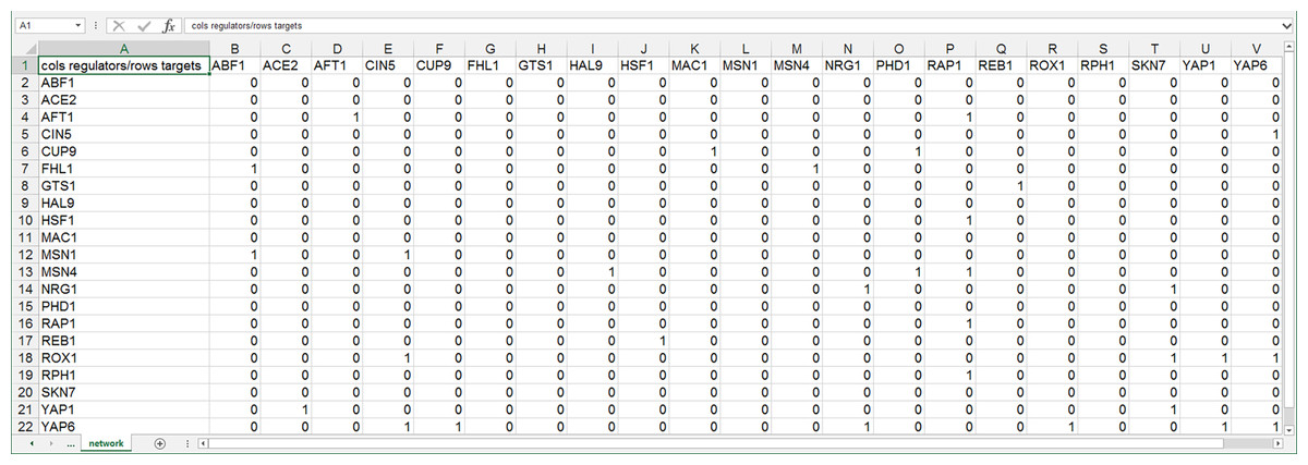
Figure 1: Screenshot of the expected format for an adjacency matrix for an unweighted network.
Regulators are named in the columns and target genes in the rows. A gene name at the top of the matrix will be considered the same as a gene name on the side if it contains the same text string, regardless of capitalization. The cells in the matrix contain a “0” if there is no regulatory relationship between the regulator and target, or a “1” if there is a regulatory relationship between them. This screenshot was generated from one of the demonstration files provided in the GRNsight user interface, Demo #3: Unweighted GRN (21 genes, 31 edges), first discussed in Dahlquist et al. (2015).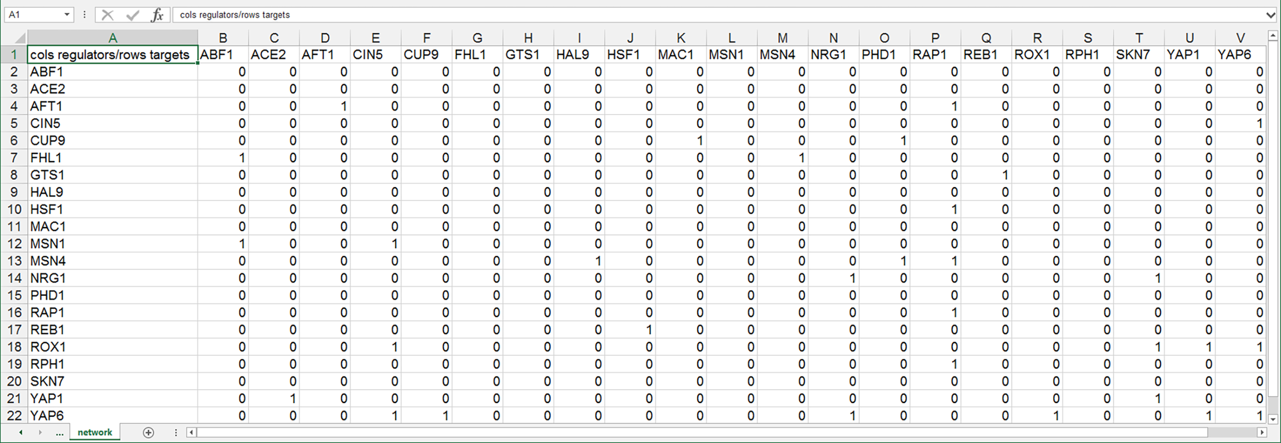
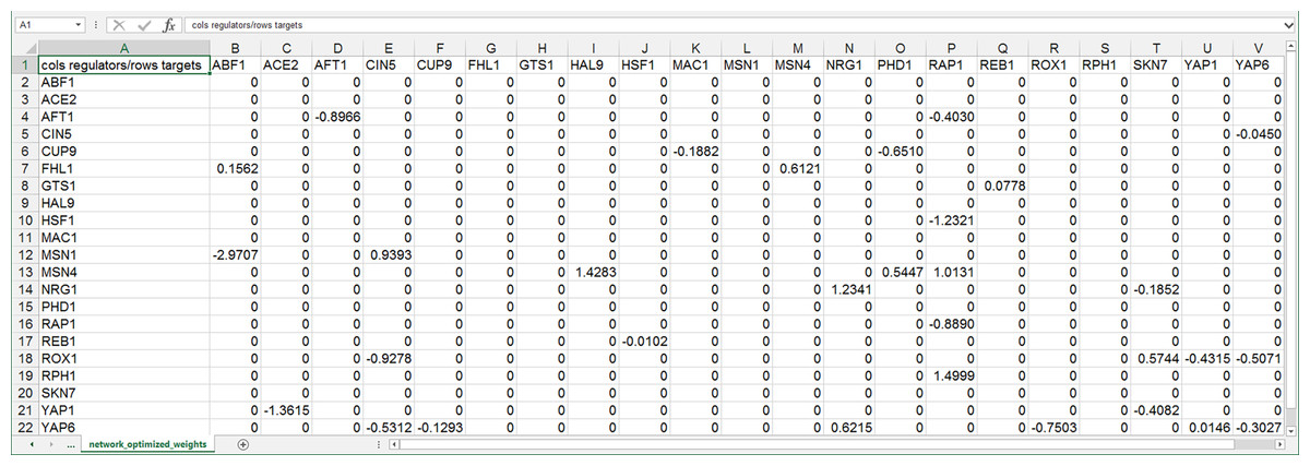
Figure 2: Screenshot of the expected format for an adjacency matrix for a weighted network.
Regulators are named in the columns and target genes in the rows. A gene name at the top of the matrix will be considered the same as a gene name on the side if it contains the same text string, regardless of capitalization. The cells in the matrix contain a “0” if there is no regulatory relationship between the regulator and target. If there is a relationship, the weight parameter is provided as a real number. Positive weights indicate activation of the target gene by the regulator, and negative weights indicate repression of the target gene by the regulator. This screenshot was generated from one of the demonstration files provided in the GRNsight user interface, Demo #4: Weighted GRN (21 genes, 31 edges; Schade et al., 2004 data), and displays weight parameters output by the GRNmap modeling software, first discussed in Dahlquist et al. (2015).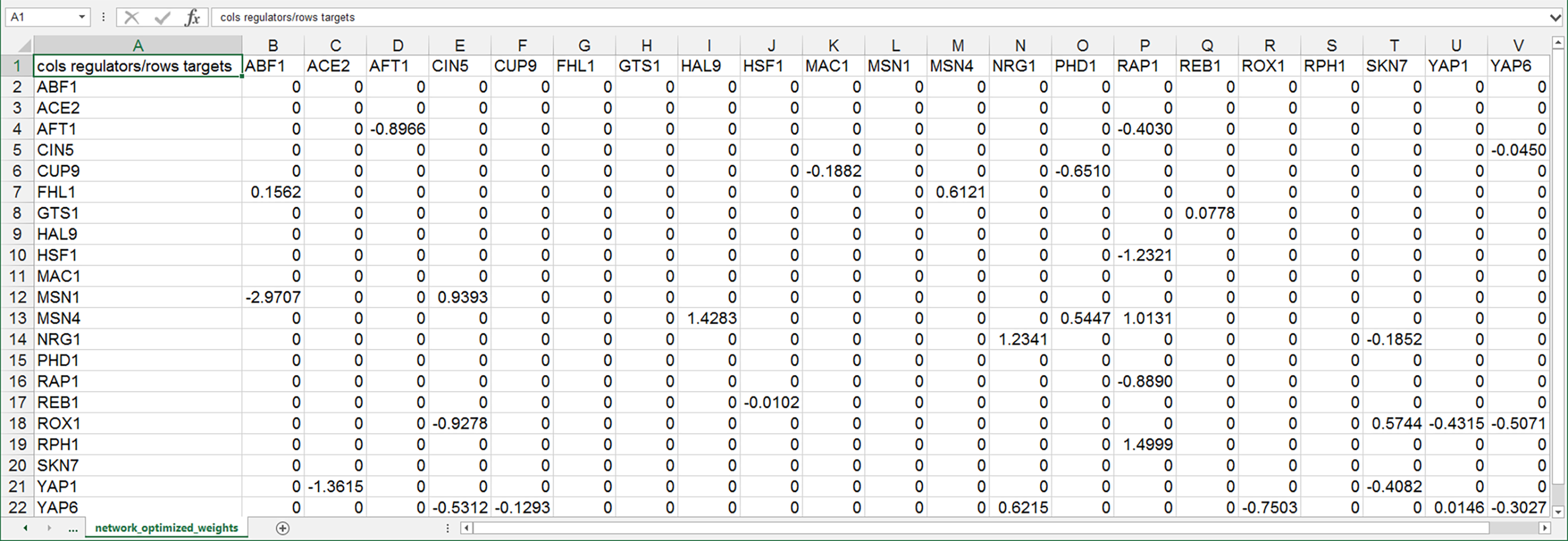
After having implemented the core functionality of seamlessly reading GRNmap-generated Excel workbooks, we recently extended the ability of GRNsight to read other commonly used network data formats to increase the interoperability of GRNsight with other network analysis and visualization software. GRNsight can import and display Simple Interaction Format (SIF, .sif, http://manual.cytoscape.org/en/latest/Supported_Network_File_Formats.html#sif-format) and GraphML (.graphml; Brandes et al., 2001; http://graphml.graphdrawing.org/) files and export network data in those two formats (see the GRNsight Documentation page for details of the implementation at http://dondi.github.io/GRNsight/documentation.html).
GRNsight is designed to visualize small- to medium-scale GRNs, not the entire GRN for an organism. The bounding box for display of the graph has a fixed size. Currently, it is recommended that the user upload networks with no more than 35 unique genes (nodes) or 70 edges. A warning is given upon upload of a network with 50–74 nodes or 71–99 edges, although the network graph will still display. If the user attempts to upload a network of 75 or more nodes or 100 or more edges, the graph does not display, and an error message will be returned.
Architecture
GRNsight has a service-oriented architecture, consisting of separate server and web client components (Fig. 3). The server provides a web application programming interface (API) that accepts a Microsoft Excel workbook (.xlsx) file via a POST request and converts it into a corresponding JavaScript Object Notation (JSON) representation. Conversion is accomplished by first parsing the .xlsx file using the node-xlsx library (https://github.com/mgcrea/node-xlsx) then mapping the translated worksheet cells into JSON. It also provides demonstration graphs already in this JSON format, without requiring a spreadsheet upload. The web client provides a graphical user interface for visualizing the JSON graphs returned by the server, whether the graphs are parsed from uploaded Excel workbooks or returned directly by the server’s demos. As an additional layer of customization, the graphical interface provided by the web client can be embedded in any web page using the standard iframe element. This is the mechanism used in deploying the production and beta versions of the software on http://dondi.github.io/GRNsight. Figure 3 illustrates this architecture and the interactions of the components.
Documentation for how GRNsight is specifically deployed, including autonomous production and beta versions, can be found on the GRNsight wiki (https://github.com/dondi/GRNsight/wiki/Server-Setup).
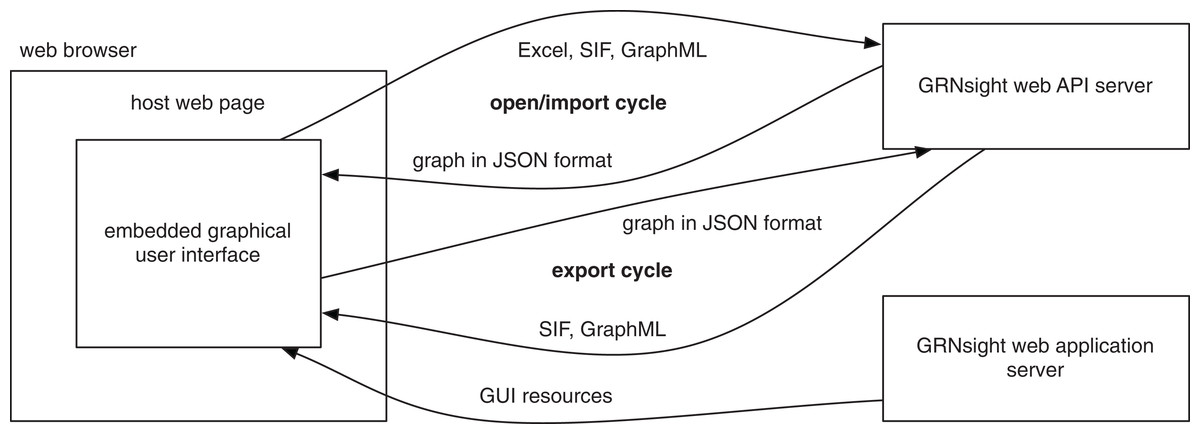
Figure 3: GRNsight architecture and component interactions.
The server provides a web API that accepts files in Microsoft Excel workbook (.xlsx), SIF (.sif), and GraphML (.graphml) formats and converts them into a unified JSON representation. A converse import function accepts this JSON representation and converts it into either SIF (.sif) or GraphML (.graphml) formats. The web application server provides code and resources for the graphical user interface that displays this JSON representation of the graph.
GRNsight is an open source project and is itself built using other open source software. Server-side components are implemented with Node.js and the Express framework (Brown, 2014). Graph visualization is facilitated by the Data-Driven Documents JavaScript library (D3.js; Bostock, Ogievetsky & Heer, 2011). D3.js provides data mapping and layout routines which GRNsight heavily customizes in order to achieve the desired graph visualization. The resulting graph is a Scalable Vector Graphics (SVG) drawing in which D3.js maps gene objects from the JSON representation provided by the web API server onto labeled rectangles. Edge weights are mapped into Bezier curves. The resulting graph is interactive, initially using D3.js’s force graph layout algorithm to automatically determine the positions of the gene rectangles. The user can then drag the rectangles to improve the graph’s layout. Customizations to the graph display are described further in the next section.
As noted in the Introduction, we decided to create our own GRNsight software instead of utilizing prior existing network visualization packages, like Cytoscape (Shannon et al., 2003; Smoot et al., 2011). However, in keeping with open source development practices, we did leverage other pre-existing code as described above. Besides D3.js, Cytoscape.js (Franz et al., 2016) has been developed as an open source network visualization engine. The BioJS registry (Yachdav et al., 2015) also lists a dozen components tagged with the keyword “network.” The choice of D3.js as the visualization engine was made simply to leverage the expertise of one of the co-authors who was already familiar with the D3.js library in order to minimize the startup, onboarding, and overhead time for the project, which initially served as a semester-long capstone experience for one of the undergraduate co-authors.
Graph customizations
GRNsight’s diagrams are based on D3.js’s force graph layout algorithm (Bostock, Ogievetsky & Heer, 2011), which was then extensively customized to support the specific needs of biologists for GRN visualization. D3.js’s baseline force graph implementation had round, unlabeled nodes and undirected, straight-line edges. The following customizations were made for the nodes: (a) the nodes were made rectangular; (b) a label of up to 12 characters was added; (c) node size was varied, depending on the size of the label.
Customizations were also made for the edges. Instead of undirected, straight line segments, the edges display as directed edges. They are implemented as Bezier curves that straighten when nodes are close together and curve when nodes are far apart. A special case was added to form a looping edge if a node regulated itself. When an unweighted adjacency matrix is uploaded, all edges are displayed as black with pointed arrowheads. When a weighted adjacency matrix is uploaded, edges are further customized based on the sign and magnitude of the weight parameter. As is common practice in biological pathway diagrams (Gostner et al., 2014), activation (for positive weights) is represented by pointed arrowheads, and repression (for negative weights) is represented by a blunt end marker, i.e., a line segment perpendicular to the edge. The thickness of the edge also varies based on the magnitude of the absolute value of the weight. Larger magnitudes have thicker edges and smaller magnitudes have thinner edges. The way that GRNsight determines the edge thickness is as follows: GRNsight divides all weight values by the absolute value of the maximum weight in the adjacency matrix to normalize all the values to between zero and one. GRNsight then adjusts the thickness of the lines to vary continuously from the minimum thickness (for normalized weights near zero) to maximum thickness (normalized weight of one). The color of the edge also imparts information about the regulatory relationship. Edges with positive normalized weight values from 0.05 to 1 are colored magenta; edges with negative normalized weight values from −0.05 to −1 are colored cyan. Edges with normalized weight values between −0.05 and 0.05 are colored grey to emphasize that their normalized magnitude is near zero and that they have a weak influence on the target gene. When a user mouses over an edge, the numerical value of the weight parameter is displayed. When the user drags nodes to customize his or her view of the network, edges adapt their anchor points to the movements of the nodes.
User interface
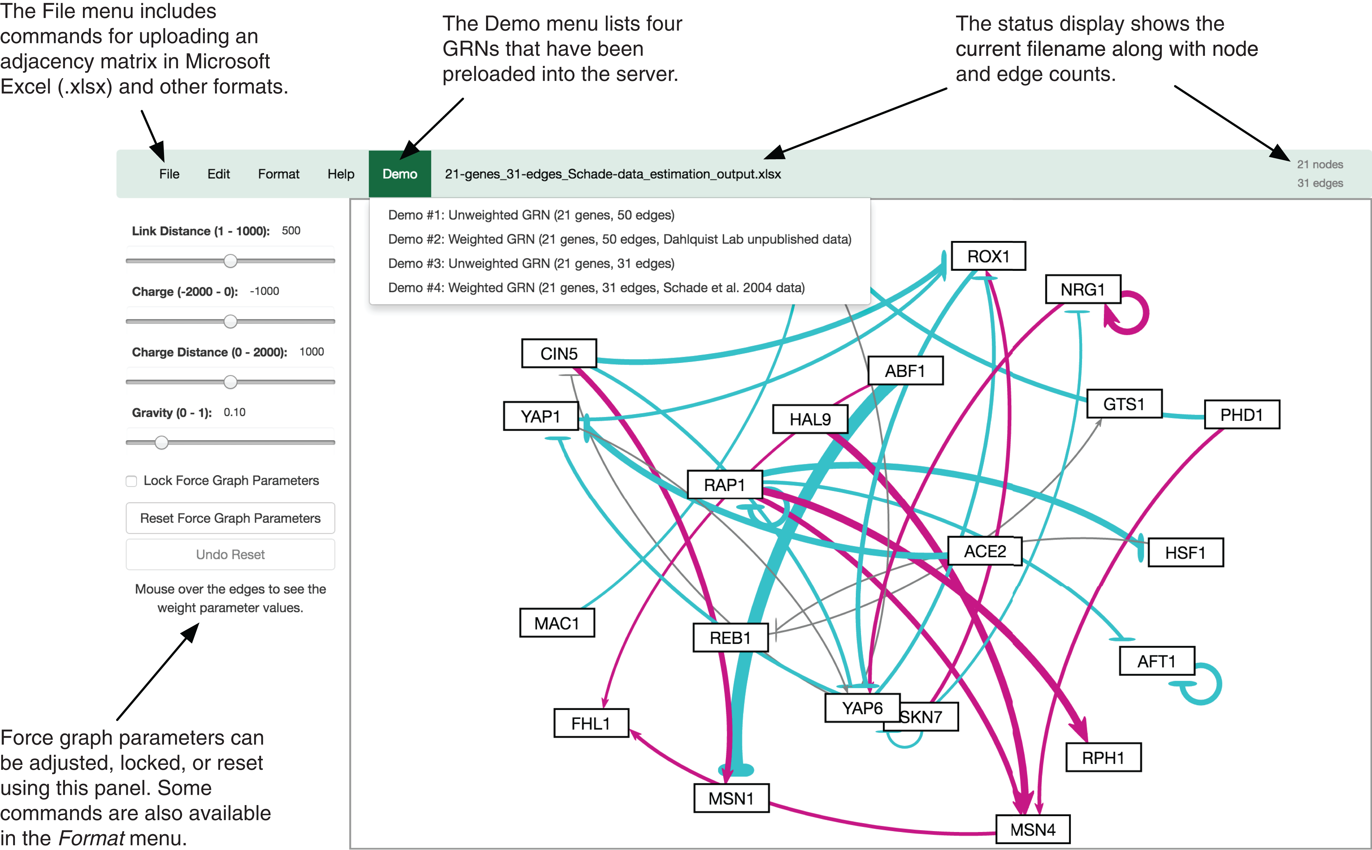
The GRNsight user interface includes a menu/status bar and sliders that adjust D3.js’s force graph layout parameters. Figure 4 provides an annotated screenshot of the user interface, highlighting its primary features. Users can move force graph parameter sliders to refine the automated visualization. Nodes have a charge, which repels or attracts other nodes. The charge distance determines at what range a node’s charge will affect other nodes. The link distance determines the minimum distance maintained between nodes. Gravity determines the strength of the force drawing the nodes to the center of the graph. Sliders can be locked to prevent changes and also reset to default values. Graph visualizations can also be modified through manual node dragging. Design decisions for the user interface were driven by applicable interaction design guidelines and principles (Nielsen, 1993; Shneiderman et al., 2016; Norman, 2013) in alignment with the mental model and expectations of the target user base, consisting primarily of biologists, both novice and experienced.
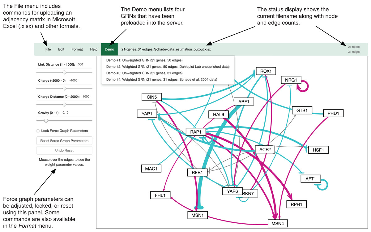
Figure 4: Annotated screenshot of the GRNsight user interface.
Test-driven development
GRNsight follows an open development model with rigorous documentation of requirements and issues on GitHub. We have implemented an exhaustive unit testing framework using Mocha (https://mochajs.org) and the Chai assertion library (http://chaijs.com) to perform test-driven development where unit tests are written before new functionality is coded (Martin, 2008). This framework consists of around 160 automated unit tests that examine nearly 530 test files to ensure that the program is running as expected. Table 1 shows the test suite’s coverage report, as generated by Istanbul (https://gotwarlost.github.io/istanbul/).
| Aspect of the code | Test coverage (percent) |
|---|---|
| Statements | 272/371 (73.3%) |
| Branches | 158/185 (85.4%) |
| Functions | 49/72 (68.1%) |
| Lines | 272/371 (73.3%) |
Error and warning messages have a three-part framework that informs the user what happened, the source of the problem, and possible solutions. This structure follows the alert elements recommended by user interface guideline documents such as the OS X human interface guidelines (https://developer.apple.com/library/mac/documentation/UserExperience/Conceptual/OSXHIGuidelines/WindowAlerts.html). For example, GRNsight returns an error when the spreadsheet is formatted incorrectly or the maximum number of nodes or edges is exceeded.
Availability
GRNsight (currently version 1.18.1) is available at http://dondi.github.io/GRNsight/ and is compatible with Google Chrome version 43.0.2357.65 or higher and Mozilla Firefox version 38.0.1 or higher on the Windows 7 and Mac OS X operating systems. The website is free and open to all users, and there is no login requirement. Website content is available under the Creative Commons Attribution Non-Commercial Share Alike 3.0 Unported License. GRNsight code is available under the open source BSD license from our GitHub repository https://github.com/dondi/GRNsight. Every user’s submitted data are private and not viewable by anyone other than the user. Uploaded data reside as temporary files and are deleted from the GRNsight server during standard operating system file cleanup procedures. A Google Analytics page view counter was implemented on 18 September 2014, and a file upload counter was added on 13 April 2015. From these start dates and as of 12 August 2016, the GRNsight home page has been accessed 2,349 times, and 1,652 files have been uploaded and viewed with GRNsight. Of these 1,652 files, an estimated 148 were uploaded by users outside of our group.
Results and Discussion
We have successfully implemented GRNsight, a web application and service for visualizing small- to medium-scale GRNs, fulfilling our five requirements:
It exists as a web application without the need to download and install specialized software;
It is simple and intuitive to use;
It accepts an input file in Microsoft Excel format (.xlsx), as well as SIF (.sif) and GraphML (.graphml);
It reads a weighted or unweighted adjacency matrix where the regulatory transcription factors are in columns and the target genes are in rows (Excel format only);
It automatically lays out and displays small- to medium-scale, unweighted and weighted, directed network graphs in a way that is familiar to biologists, adding value to the interpretation of the modeling results.
GRNsight facilitates interpretation of GRN model results
GRNsight facilitates the biological interpretation of unweighted and weighted GRN graphs. Our discussion focuses on two of the demonstration files provided in the user interface, Demo #3: Unweighted GRN (21 genes, 31 edges) and Demo #4: Weighted GRN (21 genes, 31 edges; Schade et al., 2004 data). These two files describe GRNs from budding yeast, Saccharomyces cerevisiae, correspond to supplementary data published by Dahlquist et al. (2015), and when displayed by GRNsight, represent interactive versions of Figs. 1 and 8 of that paper, respectively.
Figure 5 gives a side-by-side view of the same adjacency matrices laid out by GRNsight and by hand. Figures 5A–5C are derived from Demo #3: Unweighted GRN (21 genes, 31 edges), and Figs. 5D–5F are derived from Demo #4: Weighted GRN (21 genes, 31 edges; Schade et al., 2004 data). Figures 5A and 5D show examples of the automatic layout performed by GRNsight. Figures 5C and 5F show the same adjacency matrices laid out by hand in Adobe Illustrator, corresponding to Figs. 1 and 8 of Dahlquist et al. (2015), respectively. Figures 5B and 5E started with the automatic layout from GRNsight and then were manually manipulated from within GRNsight to lay them out similarly to Figs. 5C and 5F, respectively. The use of GRNsight represents a substantial time savings compared to creating the same figures entirely by hand and allows the user to try multiple arrangements of the nodes quickly and easily. Note that this type of “by hand” manipulation of graphs is most useful for small- to medium-scale networks, the kind that GRNsight is designed to display, and would not be appropriate for large networks.
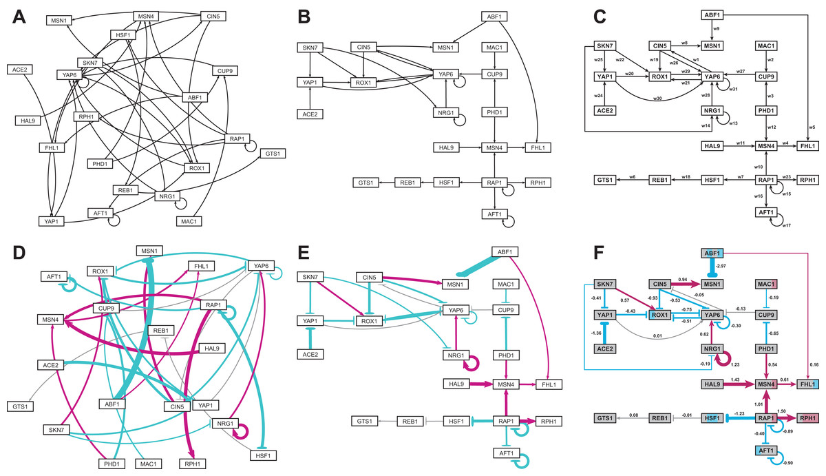
Figure 5: Side-by-side comparison of the same adjacency matrices laid out by GRNsight and by hand.
(A) GRNsight automatic layout of the demonstration file, Demo #3: Unweighted GRN (21 genes, 31 edges); (B) graph from (A) manually manipulated from within GRNsight; (C) the same adjacency matrix from (A) and (B) laid out entirely by hand in Adobe Illustrator, corresponding to Fig. 1 of Dahlquist et al. (2015); (D) GRNsight automatic layout of the demonstration file, Demo #4: Weighted GRN (21 genes, 31 edges; Schade et al., 2004 data); (E) graph from (D) manually manipulated from within GRNsight; (F) the same adjacency matrix from (D) and (E) laid out entirely by hand in Adobe Illustrator, corresponding to Fig. 8 of Dahlquist et al. (2015). The nodes in (F) are colored in the style of GenMAPP 2 (Salomonis et al., 2007), based on the time course of expression of that gene in the Schade et al. (2004) microarray data (stripes from left to right, 10, 30, and 120 minutes of cold shock, with magenta representing a significant increase in expression relative to the control at time 0, cyan representing a significant decrease in expression relative to the control, and grey representing no significant change in expression relative to the control).
Viewing the unweighted network (Figs. 5A–5C) allows one to make observations about the network structure (Dahlquist et al., 2015). For example, YAP6 has the highest in-degree, being regulated by six other transcription factors. RAP1 has the highest out-degree of five, regulating four other transcription factors and itself. Four genes, AFT1, NRG1, RAP1, and YAP6, regulate themselves. Many of the transcription factors are involved in regulatory chains, with the longest including five nodes originating at SKN7 or ACE2. There are several other four-node chains that originate at CIN5, MAC1, PHD1, SKN7, and YAP1. Finally, there are two rather complex feedforward motifs involving CIN5, ROX1, and YAP6 and SKN7, YAP1, and ROX1 (Dahlquist et al., 2015).
The networks with colored edges (Figs. 5D–5F) display the results of a mathematical model, where the expression levels of the individual transcription factors were modeled using mass balance ordinary differential equations with a sigmoidal production function and linear degradation (Dahlquist et al., 2015). Each equation in the model included a production rate, a degradation rate, weights that denote the magnitude and type of influence of the connected transcription factors (activation or repression), and a threshold of expression. The differential equation model was fit to published yeast cold shock microarray data from Schade et al. (2004) using a penalized nonlinear least squares approach. The visualization produced by GRNsight is displaying the results of the optimized weight parameters. Positive weights > 0 represent an activation relationship and are shown by pointed arrowheads. One example is that CIN5 activates the expression of MSN1. Negative weights < 0 represent a repression relationship and are shown by a blunt arrowhead. One example is that ABF1 represses the expression of MSN1. The thicknesses of the edges also vary based on the magnitude of the absolute value of the weight, with larger magnitudes having thicker edges and smaller magnitudes having thinner edges. In Figs. 5D–5F, the edge corresponding to the repression of the expression of MSN1 by ABF1 stands out as the thickest because the absolute value of its weight parameter (−2.97) has the largest magnitude out of all the weights (Dahlquist et al., 2015). It is noticeable that none of the edges that represent activation are as thick as the ABF1-to-MSN1 edge; only RAP1-to-RPH1 and HAL9-to-MSN4 are close with weights of 1.50 and 1.43, respectively.
The color of the edge also imparts information about the regulatory relationship. Edges with positive normalized weight values from 0.05 to 1 are colored magenta (10 edges in this example); edges with negative normalized weight values from −0.05 to −1 are colored cyan (16 edges in this example). Edges with normalized weight values between −0.05 and 0.05 are colored grey to indicate that their normalized magnitude is near zero and that they have a weak influence on the target gene (five edges in this example). The grey color de-emphasizes the weak relationships to the eye, thus emphasizing the stronger colored relationships.
Because of this visualization of the weight parameters, one can make some interesting observations about the behavior of the network (Dahlquist et al., 2015). Taking the arrowhead type, thickness, and color into consideration, one can, by visual inspection, group edges by type and relative influence into four activation and four repression bins. RAP1-to-RPH1, HAL9-to-MSN4, and NRG1 to itself have the strongest activation relationships, followed by RAP1-to-MSN4 and CIN5-to-MSN1, followed by NRG1-to-YAP6, MSN4-to-FHL1, SKN7-to-ROX1 and PHD1-to-MSN4, followed by ABF1-to-FHL1 as the weakest of the activation relationships. The aforementioned ABF1-to-MSN1 edge has the strongest repression relationship, followed by ACE2-to-YAP1, RAP1-to-HSF1, CIN5-to-ROX1, AFT1 to itself, and RAP1 to itself, followed by ROX1-to-YAP6, PHD1-to-CUP9, CIN5-to-YAP6, YAP6-to-ROX1, YAP1-to-ROX1, SKN7-to-YAP1, RAP1-to-AFT1, and YAP6 to itself, followed by MAC1-to-CUP9 and SKN7-to-NRG1 as the weakest of the repression relationships. These rankings could have been obtained, of course, by sorting the numerical values of the edges in a table, but it is notable that these groupings can also be picked out by eye and then put into the context of the other network connections.
Because the five weakest connections, CUP9-to-YAP6, REB1-to-GTS1, YAP6-to-CIN5, YAP1-to-YAP6, and HSF1-to-REB1, colored grey, are de-emphasized in the visual display, a different interpretation of the network structure can be made as compared to the unweighted network (Figs. 5E and 5F vs. Figs. 5B and 5C). In most cases, nodes in a regulatory chain “drop out” visually “breaking” the chain. For example, in the four-node chain beginning with RAP1-to-HSF1, the last two nodes, REB1 and GTS1, are only weakly connected. In the five-node chains beginning with SKN7-to-YAP1 or ACE2-to-YAP1, and the four-node chains beginning with MAC1-to-CUP9 or PHD1-to-CUP9, the nodes connected to YAP6 drop out (YAP1-to-YAP6, YAP6-to-CIN5, and CUP9-to-YAP6). This suggests that regulatory chains may only be effective to a depth of two levels, and that while longer chains are theoretically possible, given the network connections, they have a negligible effect on the dynamics of expression of downstream genes.
Another interpretation of the network structure that is highlighted by the weighted display is that the 21-gene network can be divided into two smaller subnetworks by removing the two edges CUP9-to-YAP6 (grey) and ABF1-to-FHL1 (thin magenta, weakly activating). While this could also be observed in the unweighted network, the application of the weight information, showing only thin connections between the two subnetworks, suggests that they could function relatively independently. Finally, the unweighted display showed two complex feedforward motifs involving CIN5, ROX1, and YAP6 and SKN7, YAP1, and ROX1. The weighted display reveals that the complexity of the connections is reduced because the weak YAP1-to-YAP6 and YAP6-to-CIN5 edges drop out. Furthermore, the display shows that the modeling predicts that the three-node CIN5-ROX1-YAP6 motif is an incoherent type 2 feedforward loop, while the SKN7-YAP1-ROX1 motif is a coherent type 4 feedforward loop, neither of which is found very commonly in Escherichia coli nor S. cerevisiae GRNs (Alon, 2007). The modeling combined with the display suggests that further investigation is warranted: either these two rare types of feedforward loops are important to the dynamics of this particular GRN, or the network structure is incorrect. In either case, future lines of experimental investigation are suggested to the user.
When examining individual genes in the network, one can see that the expression of several genes is controlled by a balance of activation and repression by different regulators. For example, the expression of MSN1 is strongly activated by CIN5, but even more strongly repressed by ABF1. The expression of ROX1 is weakly activated by SKN7 and weakly repressed by YAP1, CIN5, and YAP6. The expression of YAP6 is weakly activated by NRG1, but weakly repressed by itself, CIN5, and ROX1. Furthermore, some transcription factors act both as activators of some targets and repressors of other targets. For example, RAP1 activates the expression of MSN4 and RPH1, but represses the expression of AFT1, HSF1, and itself. PHD1, ABF1, CIN5, and SKN7 also both activate and repress their different target genes in the network. For each of these regulators, there is experimental evidence to support their opposite effects on gene expression, although not necessarily for these particular target genes (RAP1: Shore & Nasmyth, 1987; PHD1: Borneman et al., 2006, ABF1: Buchman & Kornberg, 1990 and Miyake et al., 2004; CIN5 and SKN7: Ni et al., 2009). Except for CIN5, what these genes have in common is that they themselves have no inputs in the network. The remaining no-input genes (ACE2, MAC1, and HAL9) have only one outgoing edge in this network. Because these genes have no inputs and, in some sense, have been artificially disconnected from the larger GRN of the cell, one must not overinterpret the results of the modeling for these genes.
Thus, GRNsight enables one to interpret the weight parameters more easily than one could from the adjacency matrix alone. Visual inspection has long been recognized by experts such as Tufte (2001) and Card, Mackinlay & Shneiderman (1999) as distinct from other forms of purely numeric, computational, or algorithmic data analysis, and as the preceding discussion highlights, it is this potential that can be derived specifically by visual inspection that is enabled by GRNsight. Card, Mackinlay & Shneiderman (1999) have identified six major ways, documented in earlier literature and empirical studies, by which information visualization amplifies cognition. Tufte’s (2001) seminal book perhaps states it best: “Graphics reveal data. Indeed graphics can be more precise and revealing than conventional statistical computations.”
Note that the nodes in Fig. 5F are also colored in the style of GenMAPP 2 (Salomonis et al., 2007), based on the time course of expression of that gene in the Schade et al. (2004) microarray data (stripes from left to right, 10, 30, and 120 min of cold shock, with magenta representing a significant increase in expression relative to the control at time zero, cyan representing a significant decrease in expression relative to the control, and grey representing no significant change in expression relative to the control). This feature has not yet been implemented in GRNsight, but is currently under development for Version 2.
These observations made by direct inspection of the GRNsight graph are for a relatively small GRN of 21 genes and 31 edges and become more difficult as nodes and edges are added. For much larger networks, a more powerful graph analysis tool such as Cytoscape (Shannon et al., 2003; Smoot et al., 2011) or Gephi (Bastian, Heymann & Jacomy, 2009) is warranted. However, for small networks in the range of 15–35 nodes, GRNsight fulfills a need to quickly and easily view and manipulate them. The GRN modeled in Dahlquist et al. (2015) and displayed in Fig. 5 was derived from the Lee et al. (2002) and Harbison et al. (2004) datasets generated by chromatin immunoprecipitation followed by microarray analysis. We have also used GRNsight to display GRNs derived from the YEASTRACT database (Teixeira et al., 2014), whose own display tool is static, displaying regulators and targets in two rows. Instructions for viewing YEASTRACT-derived GRNs can be found on the GRNsight Documentation page.
While GRNsight was designed originally for viewing GRNs, it is not specific for any particular species, nor for that kind of data. As long as the text strings used as identifiers for the “regulators” and “targets” match, it can be used to visualize any small, unweighted or weighted network with directed edges for systems biology or other application domains.
GRNsight development follows best practices for scientific computing and FAIR data principles
Veretnik, Fink & Bourne (2008) lament and Schultheiss et al. (2011) document that some computational biology resources, especially web servers, lack persistence and usability, leading to an inability to reproduce results. With that in mind, we have consciously followed best practices for open development (Prlić & Procter, 2012), scientific computing (Wilson et al., 2014), providing a web resource (Schultheiss, 2011), and FAIR data (Wilkinson et al., 2016), simultaneously following and teaching these practices to the primary developers who were all undergraduates. Each of these practices relates to each other, supporting reproducible research.
Open development and long-term persistence
As noted in our process requirements in the Introduction, we have followed an open development model since the project’s inception in January 2014, with our code available under the open source BSD license at the public GitHub repository, where we “release early, release often” (Torvalds in Raymond (1999)) and also track requirements, issues, and bugs. Indeed, our project stands on the shoulders of other open source tools. Our unit-testing framework provides confidence that the code works as expected. Detailed documentation for users (web page) and developers (wiki) are provided. Demo data are also provided so users have both an example of how to format input files and can see how the software should perform. As noted by Prlić & Procter (2012), open development practices have a positive impact on the long-term sustainability of a project. Furthermore, Schultheiss et al. (2011) describe twelve qualities for evaluating web services that sum to a Long-Term-Score, which correlates with persistence of the web service. GRNsight complies with all 12 requirements, providing: a stable web address (using the github.io domain to host the website and Amazon Cloud Services to host the server help to ensure long-term availability), version information, hosting country and institution, last updated date, contact information, high usability, no registration requirement, no download required, example data, fair testing possibility (both with demonstration Excel workbooks and standard SIF and GraphML file types), and a functional service.
We are committed to continue development of the GRNsight resource, fixing bugs and improving the software by adding features. The lead authors (Dahlquist, Dionisio, and Fitzpatrick) are all tenured faculty, overseeing the design, code, testing, and documentation of GRNsight and providing continuity to the project. Together we have mentored the undergraduates (Anguiano, Varshneya, Southwick, and Samdarshi) who had primary responsibility for coding, testing, and documentation, while also being full partners in the design of the software. A pipeline has been established for onboarding new members to the project, also providing continuity. Lawlor & Walsh (2015) detail some of the same issues of reliability and reproducibility in bioinformatics software referred to by Wilson et al. (2014). Lawlor & Walsh (2015) conclude that the ideal way to bring software engineering values into bioinformatics research projects is to establish separate specialists in bioinformatics engineering. We disagree. Through GRNsight, we have shown how best practices can be taught to undergraduates concomitant with training in bioinformatics, as we have shown previously with Master’s level students (Dionisio & Dahlquist, 2008).
FAIR data principles
The FAIR Guiding Principles for scientific data and stewardship state that data should be Findable, Accessible, Interoperable, and Reusable by both humans and machines (Wilkinson et al., 2016), with “data” loosely construed as any scholarly digital research object, including software. As scientific software that interacts with data, the FAIR principles can apply to both the GRNsight application and the network data it is used to visualize. Thus, we evaluate the GRNsight project in terms of its “FAIRness” below.
Findable
The Findable principle states that metadata and data should have a globally unique and persistent identifier, and that metadata and data should be registered or indexed in a searchable resource (Wilkinson et al., 2016). In terms of software, the identifier is the name and version. Because we utilize the GitHub release mechanism, GRNsight code is tagged with a version (currently v1.18.1) and each version is available from the release page (https://github.com/dondi/GRNsight/releases). We have registered GRNsight with well-known bioinformatics tools registries: the BioJS Repository (Yachdav et al., 2015; http://biojs.io/), the Elixir Tools and Data Services Registry (Ison et al., 2016; https://bio.tools/), Bioinformatics.org (http://www.bioinformatics.org/wiki/), and the Links Directory at Bioinformatics.ca (Brazas, Yamada & Ouellette, 2010; https://bioinformatics.ca/links_directory/), as well as Node Package Manager (NPM, https://www.npmjs.com/). GRNsight has also been presented at scientific conferences, with slides and posters available via SlideShare (http://www.slideshare.net/GRNsight) and with a recent talk and poster at the 2016 Bioinformatics Open Source Conference available via F1000 Research (Dahlquist et al., 2016a; Dahlquist et al., 2016b). We have paid special attention to the metadata associated with our website to increase its Findability via Google search. And, of course, with the publication of this article, GRNsight is Findable in literature databases. In the everyday sense of the word “findable,” one could argue that by being “yet another” network visualization tool in a crowded domain (recall 47 other tools recorded by Pavlopoulos et al. (2015)), GRNsight is contributing to a Findability problem for users in the sense that it contributes more “hay” to the “needle in a haystack” problem of finding the right tool for the job. However, we hope that by the actions we have taken and the specificity of our requirements for GRNsight’s functionality, publicly describing both what we mean it to be and what we do not mean it to be, the benefits of adding GRNsight to the diverse pool of network visualization software outweighs the detriments.
In addition, the Findable principle states that data should be described with rich metadata and that metadata should include the identifier of the data it describes (Wilkinson et al., 2016). Because GRNsight does not interact directly with a data repository, it is up to individual users to make sure that their data is FAIR compliant with the Findable principle. This is discussed further below with regard to Interoperability and Reusability.
Accessible
The Accessible principle states that metadata and data should be retrievable by their identifier using a standardized communication protocol, that the protocol is open, free, and universally implementable, that the protocol allows for authentication and authorization procedures, where necessary, and that metadata are accessible, even when the data are no longer available (Wilkinson et al., 2016). As noted before, GRNsight meets the first two criteria, because it is free and open to all users, and there is no login requirement. The source code is available under the open source BSD license and can be NPM installed (given the caveat that the user must be able to support the GRNsight client-server setup). The longevity of GRNsight is partially tied to the longevity of the GitHub repository itself, although the authors maintain local backups. Again, because GRNsight does not interact directly with a data repository, it is up to individual users to make sure that their data is FAIR compliant with the Accessible principle. Since GRNsight does not have any security procedures nor authentication requirements (e.g., password protection; user registration), it is not recommended that sensitive data be uploaded to our GRNsight server. However, users who wish to visualize sensitive data could run a local instance of the GRNsight client-server setup.
Interoperable
As software, GRNsight does not interact directly with other databases or software, as, for example, Cytoscape does with many pathway and molecular interaction databases or individual Cytoscape apps (formerly plugins; Saito et al., 2012), so it is not Interoperable in that sense. The GRNsight web application is designed to interact directly with a human user and is not set up to import or export data programmatically, as would be necessary to incorporate it into popular workflow environments like Galaxy (Afgan et al., 2016) or be hosted by a tool aggregator such as QUBES Hub (Quantitative Undergraduate Biology Education and Synthesis Hub, https://qubeshub.org/). However, GRNsight is Interoperable in the sense that via the user, it can receive and pass data from and to other programs. In this latter sense, this section could just as easily have been entitled, “95% of bioinformatics is getting your data into the right file format.” Indeed, one of the original motivations and requirements for GRNsight was to seamlessly read and display weighted GRNs that were output as Excel workbooks from the GRNmap MATLAB modeling package (Dahlquist et al., 2015; http://kdahlquist.github.io/GRNmap/). This specialized use case is augmented by GRNsights’s ability to import and export data in the commonly used SIF (http://manual.cytoscape.org/en/latest/Supported_Network_File_Formats.html#sif-format) and GraphML (Brandes et al., 2001; http://graphml.graphdrawing.org/) formats, facilitating movement of data between GRNsight and other network visualization and analysis programs. For instance, one can interact with the GRNsight server component directly, in order to upload Excel workbooks and supported import formats for conversion into JSON then back into a supported export format. Thus, we are in a position to comment on SIF and GraphML with respect to the finer points of data Interoperability, including: metadata and data using a formal, accessible, shared, and broadly applicable language for knowledge representation, metadata and data using vocabularies that follow the FAIR principles, and metadata and data including qualified references to other metadata and data (Wilkinson et al., 2016).
When we implemented import and export for the SIF and GraphML formats, we encountered issues due to the variations accepted by these formats which required design decisions that may, in turn, restrict compatibility with other software that we did not test. For example, the SIF format as described in the documentation for Cytoscape v3.4.0 offers quite a few divergent options, including choice of delimiter (space vs. tab), denoting a pairwise list of interactions versus concatenating all the interactions to the same node on the same line, and the choice of relationship type (any string). It only requires node identifiers to be internally consistent to the file, without enforcing the use of IDs from a recognized biological database. While GRNsight strives to read any SIF file, we restricted our export format to tab-delimited, pairwise interactions, and a single relationship type (“pd” for “protein → DNA”) for unweighted networks. For weighted networks, GRNsight exports the weight value as the relationship type. The advantage of SIF is that it is a simple text format; the main disadvantage is that all it is really intended to encode is the interaction between two nodes, which makes including the weight data as GRNsight does a kludge, and including metadata impossible. Moreover, there is no controlled vocabulary for the relationship type, only a list of suggestions in the Cytoscape documentation, from which we selected “pd.” In practice, Cytoscape v3.4.0 defaults to “interacts with” as the relationship type when exporting SIF files. As a simple text format, it does not satisfy the three sub-principles of Interoperability (Wilkinson et al., 2016).
In contrast, GraphML, as a richer XML format, has the potential to satisfy the Interoperability criteria. However, as with SIF, we encountered issues because a feature of the format that is intended to facilitate flexibility has, in practice, turned out to degrade Interoperability rather than enhance it. GraphML standardizes only the representation of nodes and edges and their directions; all other characteristics, such as names, weights, and other values, are left for others to specify through a key element, which is not subject to a controlled vocabulary. Although this flexibility is appreciated, it also serves as an enabler for divergence. In particular, two issues arose with interpreting the node identifier and display label. First, because of the lack of a controlled vocabulary, these are defined differently by different programs. Second, in the GRNsight-native Excel format, transcription factors must be unique in the header columns and rows and serve both as a unique ID for that node and the node label. In two implementations of GraphML import/export that we tested with Cytoscape v3.4.0 and a commercial graph editor called yED (v3.16, https://www.yworks.com/products/yed), an internal node ID is assigned independently of the node label and is not editable by the user. This leads to a situation where the user could assign identical labels to two or more nodes with different IDs, raising an issue for correct display of the network in GRNsight where node ID and node label are synonymous. GRNsight accommodates display of node labels from Cytoscape- and yED-exported GraphML by using a priority system to select among the XML elements it may encounter. Finally, as with SIF, there is no enforcement of the use of IDs from a recognized biological database, even though the potential exists to specify the ID source (at least as a comment) in the XML.
The format of a GraphML export by GRNsight is described on the Documentation page (http://dondi.github.io/GRNsight/documentation.html). In our testing, we have ensured that GRNsight can read Cytoscape- and yED-exported GraphML and that GRNsight-exported GraphML was accurately read by these two programs, but we cannot guarantee Interoperability with other software. Any issues that arise will need to be addressed on a case-by-case basis through bug reports at our GitHub repository.
Compliance with FAIR principles is facilitated by the BioSharing registry of standards (McQuilton et al., 2016; https://biosharing.org). As of this writing, GraphML is present in the registry, but as an unclaimed, automatically-generated entry. Other formats for sharing network data are potentially more fully FAIR compliant. However, the addition of each new format, while increasing the flexibility and power of the GRNsight software, would incur the cost of additional complexity (http://boxesandarrows.com/complexity-and-user-experience/). This is a corollary of “one thing well” and is, for example, one reason why the complex Cytoscape stand-alone application did not fit our initial product requirements. As demonstrated by our tests with Cytoscape- and yED-exported GraphML, the aphorism that “95% of bioinformatics is getting your data into the right file format” cannot entirely be avoided by developers or users.
Reusable
The FAIR principles state that metadata and data should be richly described with a plurality of accurate and relevant attributes, released with a clear and accessible usage license, associated with a detailed provenance, and meet domain-relevant community standards. As software, GRNsight is Reusable because the code is available on GitHub under the open source BSD license. The advantage of having followed test-driven development is that a developer who wishes to reuse the code has a test suite ready to guide development of new features. In terms of data, the criteria for Reusability are closely linked to Interoperability. While the GraphML format is capable of storing metadata, the limitations described above in terms of a lack of controlled vocabulary cause it to fail the Reusability test as well. In terms of provenance, GRNsight injects a comment into the GraphML recording what version of GRNsight exported the data (as does yED v3.16, but not Cytoscape v3.4.0). We also note that the GRNmap Excel workbook format with multiple worksheets has the potential to record both metadata and provenance, although this feature is not implemented at this time.
In the end, even the examples given by Wilkinson et al. (2016) have varying levels of adherence to the FAIR principles or “FAIRness,” which, they argue, should be used as a guide to the incremental improvement of resources. Although GRNsight has the limitations discussed above, we have done as much as we can to achieve FAIRness at this time.
Conclusions
We have successfully implemented GRNsight, a web application and service for visualizing small- to medium-scale GRNs that is simple and intuitive to use. GRNsight accepts an input file in Microsoft Excel format (.xlsx), reading a weighted or unweighted adjacency matrix where the regulators are in columns and the target genes are in rows, and automatically lays out and displays unweighted and weighted network graphs in a way that is familiar to biologists. GRNsight also has the capability of importing and exporting files in SIF and GraphML formats. Although GRNsight was originally developed for use with the GRNmap modeling software, and has provided useful insight into the interpretation of the GRN model described in Dahlquist et al. (2015), it has general applicability for displaying any small, unweighted or weighted network with directed edges for systems biology or other application domains. Thus, GRNsight inhabits a niche not satisfied by other software, doing “one thing well.” GRNsight also serves as a model for how best practices for software engineering support reproducible research and can be learned simultaneously with the development of useful bioinformatics software.