
Clawpack: building an open source ecosystem for solving hyperbolic PDEs
- Published
- Accepted
- Received
- Academic Editor
- Nick Higham
- Subject Areas
- Distributed and Parallel Computing, Scientific Computing and Simulation
- Keywords
- Partial differential equations, Finite volume methods, Parallel computing, Open source software, Conservation laws, Balance laws
- Copyright
- © 2016 Mandli et al.
- Licence
- This is an open access article distributed under the terms of the Creative Commons Attribution License, which permits unrestricted use, distribution, reproduction and adaptation in any medium and for any purpose provided that it is properly attributed. For attribution, the original author(s), title, publication source (PeerJ Computer Science) and either DOI or URL of the article must be cited.
- Cite this article
- 2016. Clawpack: building an open source ecosystem for solving hyperbolic PDEs. PeerJ Computer Science 2:e68 https://doi.org/10.7717/peerj-cs.68
Abstract
Clawpack is a software package designed to solve nonlinear hyperbolic partial differential equations using high-resolution finite volume methods based on Riemann solvers and limiters. The package includes a number of variants aimed at different applications and user communities. Clawpack has been actively developed as an open source project for over 20 years. The latest major release, Clawpack 5, introduces a number of new features and changes to the code base and a new development model based on GitHub and Git submodules. This article provides a summary of the most significant changes, the rationale behind some of these changes, and a description of our current development model.
Introduction
The Clawpack software suite (Clawpack Development Team, 2015) is designed for the solution of nonlinear conservation laws, balance laws, and other first-order hyperbolic partial differential equations not necessarily in conservation form. The underlying solvers are based on the wave propagation algorithms described by LeVeque in (LeVeque, 2002), and are designed for logically Cartesian uniform or mapped grids or an adaptive hierarchy of such grids. The original Clawpack was first released as a software package in 1994 and since then has made major strides in both capability and interface. More recently a major refactoring of the code and a move to GitHub for development has resulted in the release of Clawpack 5.0 in January, 2014. Beyond enabling a distributed and better managed development process, a number of user-facing improvements were made including a new user interface and visualization tools, incorporation of high-order accurate algorithms, parallelization through MPI and OpenMP, and other enhancements.
Because scientific software has become central to many advances made in science, engineering, resource management, natural hazards modeling and other fields, it is increasingly important to describe and document changes made to widely used packages. Such documentation efforts serve to orient new and existing users to the strategies taken by developers of the software, place the software package in the context of other packages, document major code changes, and provide a concrete, citable reference for users of the software.
With this in mind, the goals of this paper are to:
-
Summarize the development history of Clawpack,
-
Summarize some of the major changes made between the early Clawpack 4.x versions and the most recent version, Clawpack 5.3,
-
Summarize the development model we have adopted, for managing open source scientific software projects with many contributors, and
-
Identify how users can contribute to the Clawpack suite of tools.
This paper provides a brief history of Clawpack in ‘History of Clawpack’, a background of the mathematical concerns in ‘Hyperbolic problems,’ the modern development approach now being used in ‘Development approach,’ the major feature additions in the Clawpack 5.x major release up until Version 5.3 in ‘Advances.’ Some concluding thoughts and future plans for Clawpack are mentioned in ‘Conclusions.’
History of Clawpack
The first version of Clawpack was released by LeVeque (1994) and consisted of Fortran code for solving problems on a single, uniform Cartesian grid in one or two space dimensions, together with some Matlab (MathWorks, 2015) scripts for plotting solutions. The wave-propagation method implemented in this code provided a general way to apply recently developed high-resolution shock capturing methods to general hyperbolic systems and required only that the user provide a “Riemann solver” to specify a new hyperbolic problem. Collaboration with Berger (Berger & LeVeque, 1998) soon led to the incorporation of adaptive mesh refinement (AMR) in two space dimensions, and work with Langseth (Langseth & LeVeque, 2000; Langseth, 1996) led to three-dimensional versions of the wave-propagation algorithm and the software, with three-dimensional AMR then added by Berger.
Version 4.3 of Clawpack contained a number of other improvements to the code and formed the basis for the examples presented in a textbook (LeVeque, 2002) published in 2003. That text not only provided a complete description of the wave propagation algorithm, developed by LeVeque, but also is notable in that the codes used to produce virtually all of figures in the text were made available online (LeVeque, 2002).
In 2009, Clawpack Version 4.4 was released with a major change from Matlab to Python as the recommended visualization tool, and the development of a Python user interface for specifying the input data. Finally in January of 2013 the 4.x versions of Clawpack ended with the release of 4.6.3. 1
Version 5 of Clawpack introduces both user-exposed features and a number of modern approaches to code development, interfacing with other codes, and adding new capabilities. The move to git version control also allowed a more complete open source model. These changes are the subject of the rest of this paper.
Hyperbolic problems
In one space dimension, the hyperbolic systems solved with Clawpack typically take the form of conservation laws (1) or non-conservative linear systems (2) where subscripts denote partial derivatives and q(x, t) is a vector with m ≥ 1 components. Here the components of q represent conserved quantities, while the function f represents the flux (transport) of q. Equation (1) generalizes in a natural way to higher space dimensions; see the examples below. The coefficient matrix A in (2) or the Jacobian matrix f′(q) in (1) is assumed to be diagonalizable with real eigenvalues for all relevant values of q, x, and t. This condition guarantees that the system is hyperbolic, with solutions that are wave-like. The eigenvectors of the system determine the relation between the different components of the system, or waves, and the eigenvalues determine the speeds at which these waves travel. The right hand side of these equations could be replaced by a “source term” ψ(q, x, t) to give a non-homogeneous equation that is sometimes called a “balance law” rather than a conservation law. Spatially-varying flux functions f(q, x) in (1) can also be handled using the f-wave approach (Bale et al., 2002).
Examples of equations solved by Clawpack include:
-
Advection equation(s) for one or more tracers; in the simplest, one-dimensional case we have: The velocity field u(x, t) is typically prescribed from the solution to another fluid flow problem, such as wind. Typical applications include transport of heat, energy, pollution, smoke, or another passively-advected quantity that does not influence the velocity field.
-
The shallow water equations, describing the velocity (u, v) and surface height h of a fluid whose depth is small relative to typical wavelengths. (3) (4) (5) Here g is a constant related to the gravitational force and b(x, y) is the bathymetry, or bottom surface height. Notice that the bathymetry enters the equations through a source term; additional terms could be added to model the effect of bottom friction. These equations are used, for instance, to model inundation caused by tsunamis and dam breaks, as well as to model atmospheric flows.
-
The Euler equations of compressible, inviscid fluid dynamics, which consist of conservation laws for mass, momentum, and energy. The wave speeds depend on the local fluid velocity and the acoustic wave velocity (sound speed). Source terms can be added to include the effect of gravity, viscosity or heat transfer. These systems have important applications in aerodynamics, climate and weather modeling, and astrophysics.
-
Elastic wave equations, used to model compressional and shear waves in solid materials. Here even linear models can be complex due to varying material properties on multiple scales that affect the wave speeds and eigenvectors.
Discontinuities (shock waves) can arise in the solution of nonlinear hyperbolic equations, causing difficulties for traditional numerical methods based on discretizing derivatives directly. Modern shock capturing methods are often based on solutions to the Riemann problem that consists of equations (1) or (2) together with piecewise constant initial data with a single jump discontinuity. The solution to the Riemann problem is a similarity solution (a function of x∕t only), typically consisting of m waves (for a system of m equations) propagating at constant speed. This is true even for nonlinear problems, where the waves may be shocks or rarefaction waves (through which the solution varies continuously in a self-similar manner).
The main theoretical and numerical difficulties of hyperbolic problems involve the prescription of physically correct weak solutions and understanding the behavior of the solution at discontinuities. The Riemann solver is an algorithm that encodes the specifics of the hyperbolic system to be solved, and it is the only routine (other than problem-specific setup such as initial conditions) that needs to be changed in order to apply the code to different hyperbolic systems. In some cases, the Riemann solver may also be designed to enforce physical properties like positivity (e.g., for the water depth in GeoClaw) or to account for forces (like that of gravity) that may be balanced by flux terms.
Clawpack is based on Godunov-type finite volume methods in which the solution is represented by cell averages. Riemann problems between the cell averages in neighboring states are used as the fundamental building block of the algorithm. The wave-propagation algorithm originally implemented in Clawpack (and still used in much of the code) is based on using the waves resulting from each Riemann solution together with limiter functions to achieve second-order accuracy where the solution is smooth together with sharp resolution of discontinuities without spurious numerical oscillations (see LeVeque (2002) for a detailed description of the algorithms). Higher-order WENO methods have also been developed relying on the same Riemann solvers. These methods can be found in PyClaw (see ‘PyClaw’), one of the packages in the larger Clawpack ecosystem.
Problem-specific boundary conditions must also be imposed, which are implemented by a subroutine that sets the solution value in ghost cells exterior to the domain each time step. The Clawpack software contains library routines that implement several sets of boundary conditions that are commonly used, e.g., periodic boundary conditions, reflecting solid wall boundary conditions for problems such as acoustics, Euler, or shallow water equations, and non-reflecting (absorbing) extrapolation boundary conditions. As with all Clawpack library routines, the boundary condition routine can be copied and modified by the user to implement other boundary conditions needed for a particular application.
In two or three space dimensions, the wave-propagation methods are extended using either dimensional splitting, so that only one-dimensional Riemann solvers are needed, or by a multi-dimensional algorithm based on transverse Riemann solvers introduced in (LeVeque, 1997). Both approaches are supported in Clawpack. A variety of Riemann solvers have been developed for Clawpack, many of which are collected in the riemann repository, see ‘Riemann: a community-driven collection of approximate riemann solvers.’
Adaptive mesh refinement (AMR) is essential for many problems and has been available in two space dimensions since 1995, when Marsha Berger joined the project team and her AMR code for the Euler equations of compressible flow was generalized to fit into the software which became AMRClaw (Berger & LeVeque, 1998), another package included in the Clawpack ecosystem. AMRClaw was carried over to three space dimensions using the unsplit algorithms introduced in (Langseth & LeVeque, 2000). Starting in Version 5.3.0, dimensional splitting is also supported in AMRClaw, which can be particularly useful in three space dimensions where the unsplit algorithms are much more expensive. Other recent improvements to AMRClaw are discussed in ‘AMRClaw.’
There are several other open source software projects that provide adaptive mesh refinement for hyperbolic PDEs. The interested reader may want to investigate AMROC (Deiterding, 2011), BoxLib (https://ccse.lbl.gov/BoxLib/index.html), Chombo (Adams et al., 2014), Gerris (Popinet, 2001), OpenFOAM (OpenFOAM Foundation, 2016), or SAMRAI (Anderson et al., 2013), for example.
Development Approach
Clawpack’s development model is driven by the needs of its developer community. The Clawpack project consists of several interdependent projects: core solver functionality, a visualization suite, a general adaptive mesh refinement code, a specialized geophysical flow code, and a massively parallel Python framework. Changes to the core solvers and visualization suite have a downstream effect on the other codes, and the developers largely work in an independent, asynchronous manner across continents and time zones.
The core Clawpack software repositories are:
-
clawpack–responsible for installation and coordination of other repositories,
-
riemann–Riemann solvers used by all the other projects,
-
visclaw–a visualization suite used by all the other projects,
-
clawutil–utility functions used by most other projects,
-
classic–the original single grid methods in 1, 2, and 3 space dimensions,
-
amrclaw–the general adaptive mesh refinement framework in 2 and 3 dimensions,
-
geoclaw–solvers for depth-averaged geophysical flows which employs the framework in amrclaw, and
-
pyclaw–a Python implementation and interface to the Clawpack algorithms including high-order methods and massively parallel capabilities.
A release of Clawpack downloaded by users contains all of the above. The repositories riemann, visclaw, and clawutil are sometimes referred to as upstream projects, since their changes affect all the remaining projects in the above list, commonly referred to as downstream projects. There are some variations on this, for instance AMRClaw is upstream of GeoClaw, which uses many of the algorithms and software base from AMRClaw. To coordinate this the clawpack repository points to the most recent known-compatible version of each repository.
Beyond the major core code repositories, additional repositories contain documentation and extended examples for using the packages:
-
doc–the primary documentation source files. These files are written in the markup language reStructured Text (http://www.sphinx-doc.org/en/stable/rest.html), and are then converted to html files using Sphinx (http://sphinx-doc.org). Other documentation such as drafts of this paper are also found in this repository.
-
clawpack.github.com–the html files created by Sphinx in the doc repository are pushed to this repository, and are then automatically served on the web. These appear at http://www.clawpack.org, which is configured to point to http://clawpack.github.com. The name of this repository follows GitHub convention for use with GitHub Pages (https://pages.github.com/).
-
apps–applications contributed by developers and users that go beyond the introductory examples included in the core repositories.
The Clawpack 4.x code is also available in the repository clawpack-4.x but is no longer under development.
Version control
The Clawpack team uses the Git distributed version control system to coordinate development of each major project. The repositories are publicly coordinated under the Clawpack organization on GitHub (https://github.com/clawpack) with the top-level clawpack super-repository responsible for hosting build and installation tools, as well as providing a synchronization point for the other repositories. The remaining “core Clawpack repositories” listed above are subrepositories of the main clawpack organization.
GitHub itself is a free provider of public Git repositories. In addition to repository hosting, the Clawpack team uses GitHub for issue tracking, code review, automated continuous integration via Travis CI (https://travis-ci.org/), and test coverage tracking via Coveralls (http://coveralls.io) for the Python-based modules. The issue tracker on GitHub supports cross-repository references, simplifying communication between Clawpack developer sub-teams. The Travis CI service, which provides free continuous integration for publicly developed repositories on GitHub, runs Clawpack’s test suites through nose (https://nose.readthedocs.org) on proposed changes to the code base, and through a connection to the Coveralls service, reports on any test failures as well as changes to test coverage.
Submodules
The clawpack “super-repository” serves two purposes. First, it contains installation utilities for each of the sub-projects. Second, it serves as a synchronization point for the project repositories. The remainder of this section provides more details on how Git submodules enable this synchronization.
Whenever possible, teams of software developers coordinate their development in a single unified repository. In situations where this isn’t possible, one option provided by Git is the submodule, which allows a super-repository (in this case, clawpack), to nest sub-repositories as directories, with the ability to capture changes to sub-repository revisions as new revisions in the super-repository. Under the hood, the super-repository maintains pointers to the location of each submodule and its current revision. The submodule directories contain normal Git repositories, all of the coordination happens in the super-repository.
Each of the other core Clawpack repositories listed above is a submodule of the clawpack repository. Every commit that creates a new revision to the clawpack repository describes top-level installation code as well as the revisions of each of the submodules. In this way, Git submodules allow Clawpack team members to work asynchronously on independent projects while reusing and maintaining common software infrastructure.
Typically the Clawpack developers advance the master development branch of the top-level clawpack repository any time a major feature is added or a bug is fixed in one of the upstream projects that might affect code in other repositories. By checking out a particular revision in the clawpack repository and performing a git submodule update, all repositories can be updated to versions that are intended to be consistent and functional.
In particular, when Travis CI runs the regression tests in any project repository (performed automatically for any pull request), it starts by installing Clawpack on a virtual machine and the current head of the clawpack/master branch indicates the commit from each of the other projects that must be checked out before performing the tests. If the clawpack repository has not been properly updated following changes in other upstream projects, these tests may fail.
Any new release of Clawpack is a snapshot of one particular revision of clawpack and the related revisions of all submodules. These particular revisions are also tagged for future reference with consistent names, such as v5.3.1. (Git tags simply provide a descriptive name for a particular revision rather than having to refer to a Git hash code.)
Contributing
Scientists who program are often discouraged from sharing code due to existing reward mechanisms and the fear of being “scooped.” However, recent studies indicate that scientific communities that openly share and develop code have an advantage because each researcher can leverage the work of many others (Turk, 2013), and that paper citation rates can be increased by sharing code (Vandewalle, 2012) and/or data (Piwowar, Day & Fridsma, 2007). Moreover, journals and funding agencies are increasingly requiring investigators to share code used to obtain published results. One of the goals of the Clawpack project is to facilitate code sharing by users, by providing an easy mechanism to refer to a specific version of the Clawpack software and ensuring that past versions of the software remain available on a stable and citable platform.
On the development side, we expect that the open source development model with important discussions conducted in public will lead to further growth of the developer community and additional contributions from users. Over the past twenty years, many users have written code extending Clawpack with new Riemann solvers, algorithms, or domain-specific problem tools. Unfortunately, much of this code did not make it back into the core software for others to use. Many of the development changes in Clawpack 5.x were done to encourage contributions from a broader community. We have begun to see an increase in contributions from outside the developers’ groups, and hope to encourage more of this in the future.
The primary development model is typical for GitHub projects: a contributor forks the repository on GitHub, then develops improvements in a branch that is pushed to her own fork. She issues a “pull request” (PR) when the branch is ready to be merged into the main repository. Increasingly, contributors are also using PRs as a way to conveniently post preliminary or prototype code for discussion prior to further development, often marked WIP for “work in progress” to signal that it is not ready to merge.
After a PR is issued, other developers, including one or more of the maintainers for the corresponding project, review the code. The Travis CI server also automatically runs the tests on the proposed new code. The test results are visible on the GitHub page for the PR. Usually there is some iteration as developers suggest improvements or discuss implementation choices in the code. Once the tests are passing and it is agreed that the code is acceptable, a maintainer merges it.
An additional benefit of using the GitHub platform is that any version of the code is accessible either through the command line git interface, through the GitHub website, or a number of available applications on all widely used platforms. More important however is the ability to tag a particular version of a repository with a digital object identifier (DOI) via GitHub and Zonodo.2 The combination of these abilities provides the capability for Clawpack to not only be accessible at any version but also allows for the citability of versions of the code used for particular results within the scientific literature.
Releases
Although Clawpack is continuously developed, it is convenient for users to be able to install stable versions of the software. The Clawpack developers provide these releases through two distribution channels: GitHub and the Python Package Index (PyPI). Full source releases are available on GitHub. Alternatively, the PyClaw subproject and its dependencies can be installed automatically using a PyPI client such as pip.
Clawpack does not follow a calendar release cycle. Instead, releases emerge when the developer community feels enough changes have accumulated since the last release to justify the cost of switching to a new release. For the most part, Clawpack releases are versioned using an M.m.p triplet, representing the major (M), minor (m), and patch (p) versions respectively. In the broader software engineering community, this is often referred to as semantic versioning. Small changes that fix bugs and cosmetic issues result in increments to the patch-level. Backwards-compatible changes result in an increase to the minor version. The introduction of backwards-incompatible changes require that the major version be incremented. In addition, the implementation of significant new algorithms or capability will also justify the increment of major release number, and is often an impetus for providing another release to the public. In practice, the Clawpack software has frequently included changes in minor version releases that were not entirely backwards compatible, but these have been relatively minor and documented in the release notes. Major version numbers have changed infrequently and related to major refactoring of the code as in going from 4.x to 5.0.
Staring with Version 5.3.1, the tarfiles for Clawpack releases will also be archived on Zenodo (https://zenodo.org), a data repository hosted at CERN that issues DOIs so that the software version can be cited with a permanent link (Clawpack Development Team, 2015) that does not depend on the long-term existence of GitHub.
Dependencies
Running any part of Clawpack requires a Python interpreter and the common Python packages numpy (Jones et al., 2001), f2py (Peterson, 2009), matplotlib (Hunter, 2007), as well as (except for the pure-Python 1D code) GNU make and a Fortran compiler. Other dependencies are optional, depending on which parts of Clawpack are to be used:
-
IPython/Jupyter if using the notebook interfaces (Pérez & Granger, 2007).
-
PETSc (Balay et al., 2010), if using distributed parallelism in PyClaw.
-
OpenMP, if using shared-memory parallelism in AMRClaw or GeoClaw.
-
MATLAB, if using the legacy visualization tools.
Advances
This section describes the major changes in each of the code repositories in moving from Clawpack 4.x to the most recent version 5.3. A number of the repositories have seen only minor changes as the bulk of the development is focused on current research interests. There are a number of minor changes not listed here and the interested reader is encouraged to refer to the change logs (http://www.clawpack.org/changes.html) and the individual Clawpack Git repositories for a more complete list.
Global Changes
Substantial redesign of the Clawpack code base was performed in the move from Clawpack 4.x to 5.x. Major changes that affected all aspects of the code include:
-
The interface to the Clawpack Riemann solvers was changed so that one set of solvers can be used for all versions of the code (including PyClaw via f2py (http://docs.scipy.org/doc/numpy-dev/f2py)). Rather than appearing in scattered example directories, these Riemann solvers have all been collected into the new riemann repository. Modifications to the calling sequences were made to accommodate this increased generality.
-
Calling sequences for a number of other Fortran subroutines were also modified based on experiences with the Clawpack 4.x code. These can also be used as a stand-alone product for those who only want the Riemann solvers.
-
Python front-ends were redesigned to more easily specify run-time options for the solver and visualization. The Fortran variants (ClassicClaw, AMRClaw, and GeoClaw) all use a Python script to facilitate setting input variables. These scripts create text files with a rigidly specified format that are then read in when the Fortran code is run. The interface now allows updates to the input parameters while maintaining backwards compatibility.
-
The indices of the primary conserved quantities were reordered. In Clawpack 4.x, the mth component of a system of equations in grid cell (i, j) (in two dimensions, for example), was stored in q(i,j,m). In order to improve cache usage and to more easily interface with PETSc (Balay et al., 2010), a global change was made to the ordering so that the component number comes first; i.e., q(m,i,j). A seemingly minor change like this affects a huge number of lines in the code and cannot easily be automated. The use of version control and regression tests was crucial in the successful completion of the project.
Riemann: a community-driven collection of approximate riemann solvers
The methods implemented in Clawpack, and all modern Godunov-type methods for hyperbolic PDEs, are based on the solution of Riemann problems as discussed in ‘Hyperbolic Problems.’ Whereas most existing codes for hyperbolic PDEs use Riemann solvers to compute fluxes, Clawpack Riemann solvers instead compute the waves (or discontinuities) that make up the Riemann solution. In the unsplit algorithm, Clawpack also makes use of transverse Riemann solvers, responsible for computing transport between cells that are only corner (in 2d) or edge (in 3d) adjacent.
For nonlinear systems, the exact solution of the Riemann problem is computationally costly and may involve both discontinuities (shocks and contact waves) and rarefactions. It is almost always preferable to employ inexact Riemann solvers that approximate the solution using discontinuities only, with an appropriate entropy condition. The solvers available in Clawpack are all approximate solvers, although one could easily implement their own exact solver and make it available in the format needed by Clawpack routines.
A common feature in all packages in the Clawpack suite is the use of a standard interface for Fortran Riemann solver routines. This ensures that new solvers or solver improvements developed for one package can immediately be used by all packages. To further facilitate this sharing and to avoid duplication, Riemann solvers are (with rare exceptions) not maintained under the other packages but are collected in a single repository named riemann. Users who develop new solvers for Clawpack are encouraged to submit them to the Riemann repository.
In the Fortran-based packages (Classic, AMRClaw, and GeoClaw) the Riemann solver is selected at compile-time by modifying a problem-specific Makefile. In PyClaw, the Riemann solver to be used is selected at run-time. This is made possible by compiling all of the Riemann solvers (when PyClaw is installed) and generating Python wrappers with f2py. For PyClaw, riemann also provides metadata (such as the number of equations, the number of waves, and the names of the conserved quantities) for each solver so that setup is made more transparent.
Classic
The classic repository contains code implementing the wave propagation algorithm on a single uniform grid, in much the same form as the original Clawpack 1.0 version of 1994 but with various enhancements added through the years. Following the introduction of Clawpack 4.4 the three-dimensional routines were left out of the Python user interfaces and plotting routines. These have been reintroduced in Clawpack 5. Additionally the OpenMP shared-memory parallelism capabilities have been extended to the three-dimensional code. 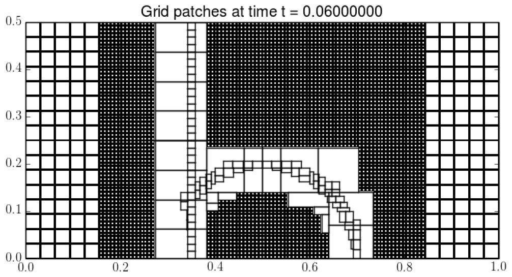
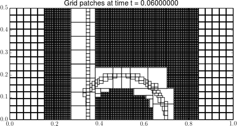
Figure 1: An illustration showing grid cells on levels one and two, and only grid outlines on levels three and four.
AMRClaw
Fortran code in the AMRClaw repository performs block-structured adaptive mesh refinement (Berger & Oliger, 1984; Berger & Colella, 1989) for both Clawpack and GeoClaw applications. The algorithms implemented in AMRClaw are discussed in detail in (Berger & LeVeque, 1998; LeVeque, George & Berger, 2011), but a short description is given here to set the stage for a description of recent changes. This type of refinement solves the PDE on a hierarchy of logically rectangular grids. One (or more) level 1 grids comprise the entire domain, while grids at finer level are created and destroyed (as opposed to moving these grids) to follow important features in the solution (see Fig. 1).
AMRClaw includes the functionality for:
-
Coordinating the flagging of points where refinement is needed, with a variety of criteria possible for flagging cells that need refinement from each level to the next finer level (including Richardson extrapolation, gradient testing, or user-specified criteria; see http://www.clawpack.org/flag.html),
-
Organizing the flagged points into efficient grid patches at the next finer level, using the algorithm of (Berger & Rigoutsos, 1991),
-
Interpolating the solution to newly created fine grids and initializing auxiliary data (topography, wind velocity, metric data and so on) on these grids,
-
Averaging fine grid solutions to coarser grids,
-
Orchestrating the adaptive time stepping (i.e., sub-cycling in time),
-
Interpolating coarse grid solution to fine grid ghost cells, and
-
Maintaining conservation at patch boundaries between resolution levels.
AMRClaw now allows users to specify “regions” in space–time [x1, x2] × [y1, y2] × [t1, t2] in which refinement is forced to be at least at some level L1 and is allowed to be at most L2. This can be useful for constraining refinement, e.g., allowing or ensuring resolution of only a small coastal region in a global tsunami simulation. Previously the user could enforce such conditions by writing a custom flagging routine, but now this is handled in a general manner so that the parameters above can all be specified in the Python problem specification. Multiple regions can be specified, and a simple rule is used to determine the constraints at a grid cell that lies in multiple regions.
Auxiliary arrays are often used in Clawpack to store data that describes the problem and the routine. The routine setaux must then be provided by the user to set these values each time a new grid patch is created. For some applications, computing these values can be time-consuming. In Clawpack 5.2, this code was improved to allow reuse of values from previous patches at the same level where possible at each regridding time. This is backward compatible, since no harm is done if previously written routines are used that still compute and overwrite instead of checking a mask.
In Clawpack 5.3 the capability to specify spatially varying boundary conditions was added. For a single grid, it is a simple matter to compute the location of the ghost cells that extend outside the computational domain and set them appropriately. With AMR however, the boundary condition routine can be called for a grid located anywhere in the domain, and may contain fewer or larger numbers of ghost cells. For this reason, the boundary condition routines do not assume a fixed number of ghost cells.
Anisotropic refinement is allowed in both two and three dimensions. This means that the spatial and temporal refinement ratios can be specified independently from one another (as long as the temporal refinement satisfies the CFL condition). In addition, capabilities have been added to automatically select the refinement ratio in time on each level based on the CFL condition. This has only been implemented in GeoClaw where the wave speed in the shallow water equations depends on the local depth. The finest grids are often located only in shallow coastal regions, so a large refinement ratio in space does not lead to a large refinement ratio in time.
AMRClaw has been parallelized using OpenMP directives. The main paradigm in structured AMR is an outer loop over levels of refinement, and an inner loop over all grids at that level, where the same operation is performed on each grid (i.e., taking a time step, finding ghost cells, conservation updates, etc.). This inner loop is parallelized using a parallel for loop construct one thread is assigned to operate on one grid. Dynamic scheduling is used with a chunk size of one. To help with load balancing, grids at each level are sorted from largest to smallest, using the total number of cells in the grid as an indicator of work. In addition the grids are limited to a maximum of 32 cells in each dimension, otherwise they are bisected until this condition is met. Note that this approach causes a memory bulge. Each thread must have its own scratch arrays to save the incoming and outgoing waves and fluxes for future conservation fix-ups. The bulge is directly proportional to the number of threads executing. For stack-based memory allocation per thread, the use of the environment variable OMP_STACKSIZE to increase the limit may be necessary.
Figure 2 shows two snapshots of the solution to a three-dimensional shock-bubble interaction problem found in the Clawpack apps repository, illustrating localized phenomena requiring adaptive refinement. In Fig. 3 we show scalability tests and some timings for this example, when run on a 24 core Intel Xeon Haswell machine (E5-2670v3 at 2.3 GHz), using KMP_AFFINITY compact with one thread per core. For timing purposes, the only modifications made to the input parameters was to turn off check-pointing and graphics output. The plot on the left shows that most of the wall clock time is in the integration routine (stepgrid), which closely tracks the total time. The second chunk of time is in the regridding, which contains algorithms that are not completely scalable. Very little time is in the filling of ghost cells, mostly from other patches but also includes those at domain boundaries. The efficiency is above 80% until 24 cores. Note that there are only two grids on level 1, and an average of 22.8 level 2 grids. Most of the work is on level 3 grids, where there are an average of 138.1 grids over all the level 3 timestep. At 24 cores, there are on average 5.8 grids per core, and the grids are very different sizes.
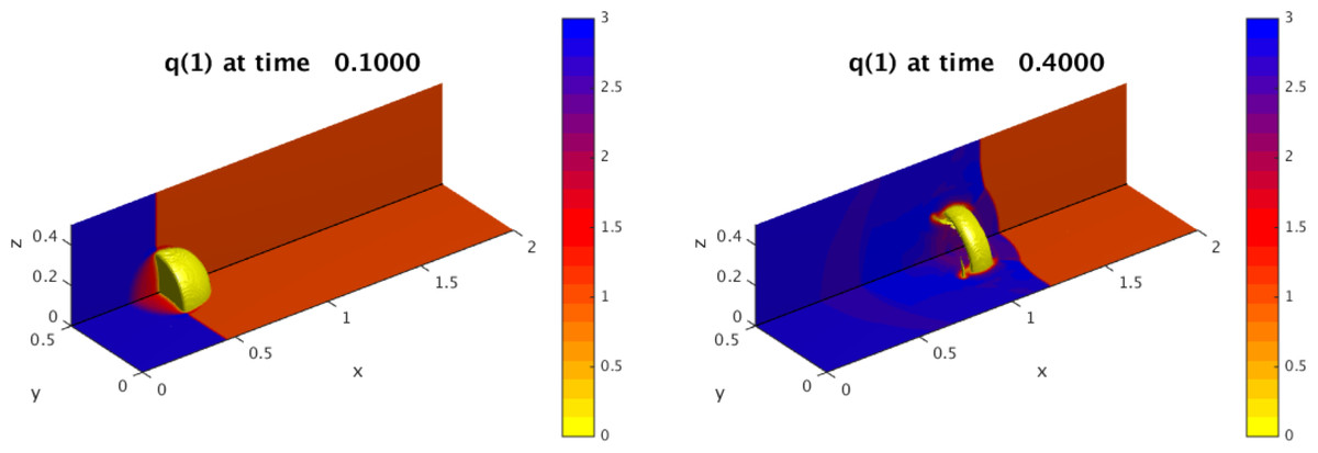
Figure 2: AMRClaw example demonstrating a shock-bubble interaction in the Euler equations of compressible gas-dynamics at two times, illustrating the need for adaptive refinement to capture localized behavior.
There are two 20 × 10 × 10 grids at level 1. They are refined where needed by factors of 4 and then 2 in this 3-level run.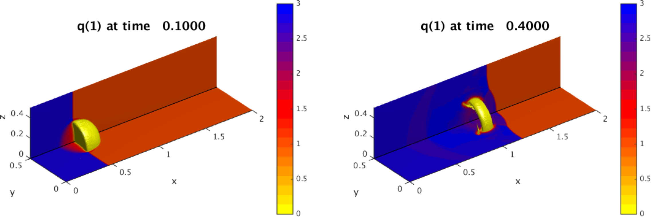
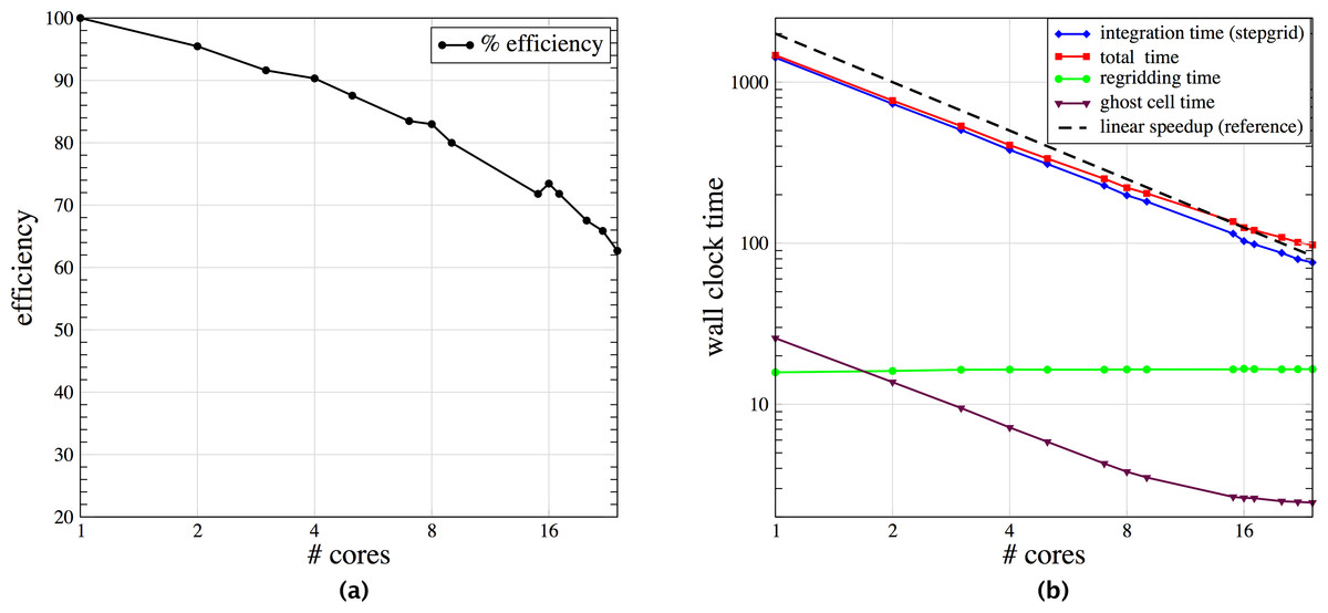
Figure 3: Scaling Results for AMRClaw.
(A) is strong scaling results for the AMRClaw example shown in Fig. 2. (B) is plot of efficiency based on total computational time.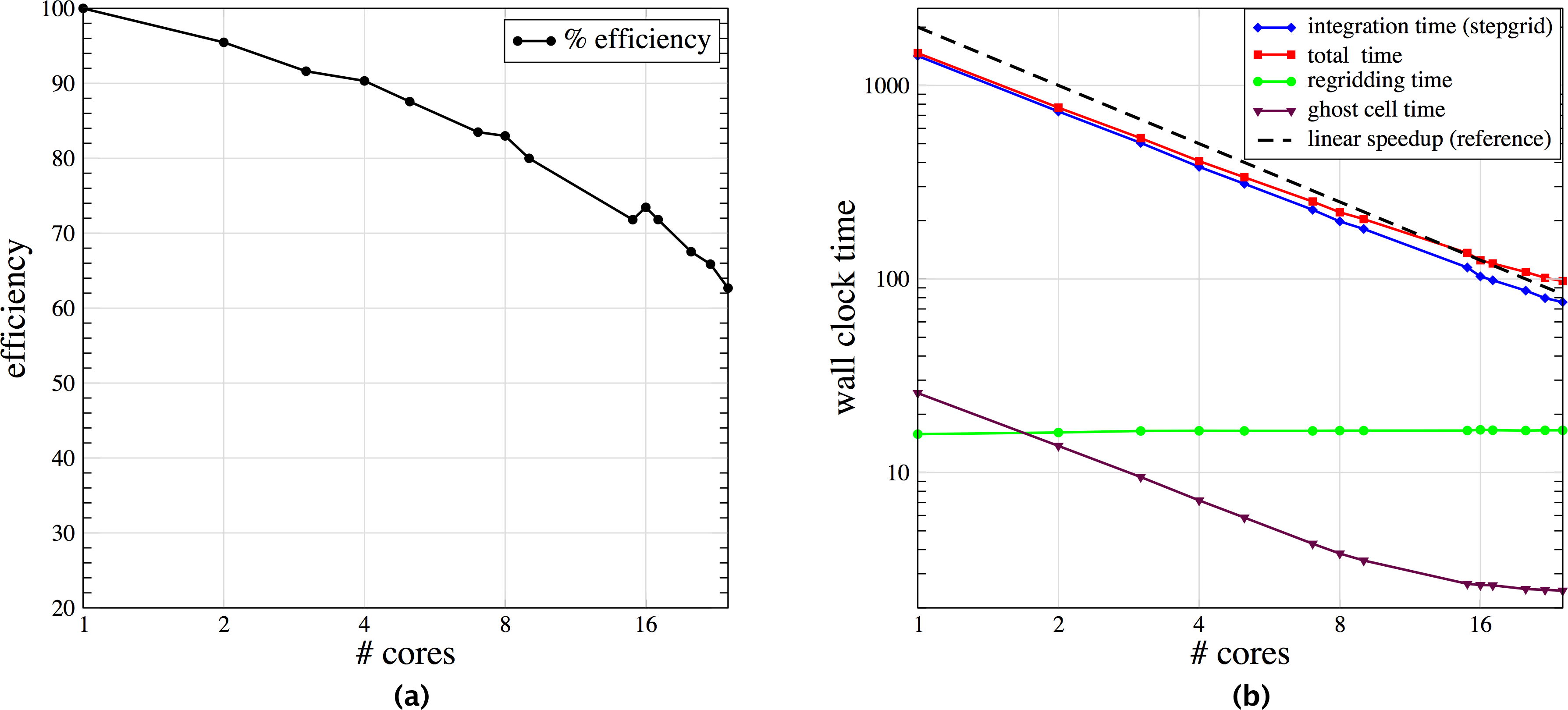
The target architecture for AMRClaw and GeoClaw are multi-core machines. PyClaw on the other hand scales to tens of thousands of cores using MPI via PETSc (Balay et al., 2010) but is not adaptive.
GeoClaw
The GeoClaw branch of Clawpack was developed to solve the two-dimensional shallow water equations over topography for modeling tsunami generation, propagation, and inundation. The AMRClaw code formed the starting point but it was necessary to make many modifications to support the requirements of this application, as described briefly below. This code originated with the work of George (George, 2004; George, 2006; George, 2008) and was initially called TsunamiClaw. Later it became clear that many other geophysical flow applications have similar requirements and the code was generalized as GeoClaw.
One of the major issues is the treatment of wetting and drying of grid cells at the margins of the flow. The handling of dry states in a Riemann solver is difficult to handle robustly, and has gone through several iterations. GeoClaw must also be well-balanced in order to preserve steady states, in particular the “ocean at rest.” To achieve this, the source terms in the momentum equations arising from variations in topography are incorporated into the Riemann solver rather than using a fractional step splitting approach. This is critical for modeling waves that have very small amplitudes relative to the variations in the depth of the ocean. See LeVeque (2010) for a general discussion of such methods and George (2006) and George (2008) for details of the Riemann solver used in GeoClaw. Other features of GeoClaw include the ability to solve the equations in latitude–longitude coordinates on the surface of the sphere, and the incorporation of source terms modeling bottom friction using a Manning formulation. More details about the code and tsunami modeling applications can be found in (Berger et al., 2011; LeVeque, George & Berger, 2011). In 2011, a significant effort took place to verify and validate GeoClaw against the US National Tsunami Hazard Mitigation Program (NTHMP) benchmarks (González et al., 2011). NTHMP approval of the code allows GeoClaw to be used in hazard mapping projects that are funded by this program or other federal and state agencies, e.g., (González, LeVeque & Adams, 2013; Gonzalez et al., 2014). One such project is illustrated in Fig. 4.
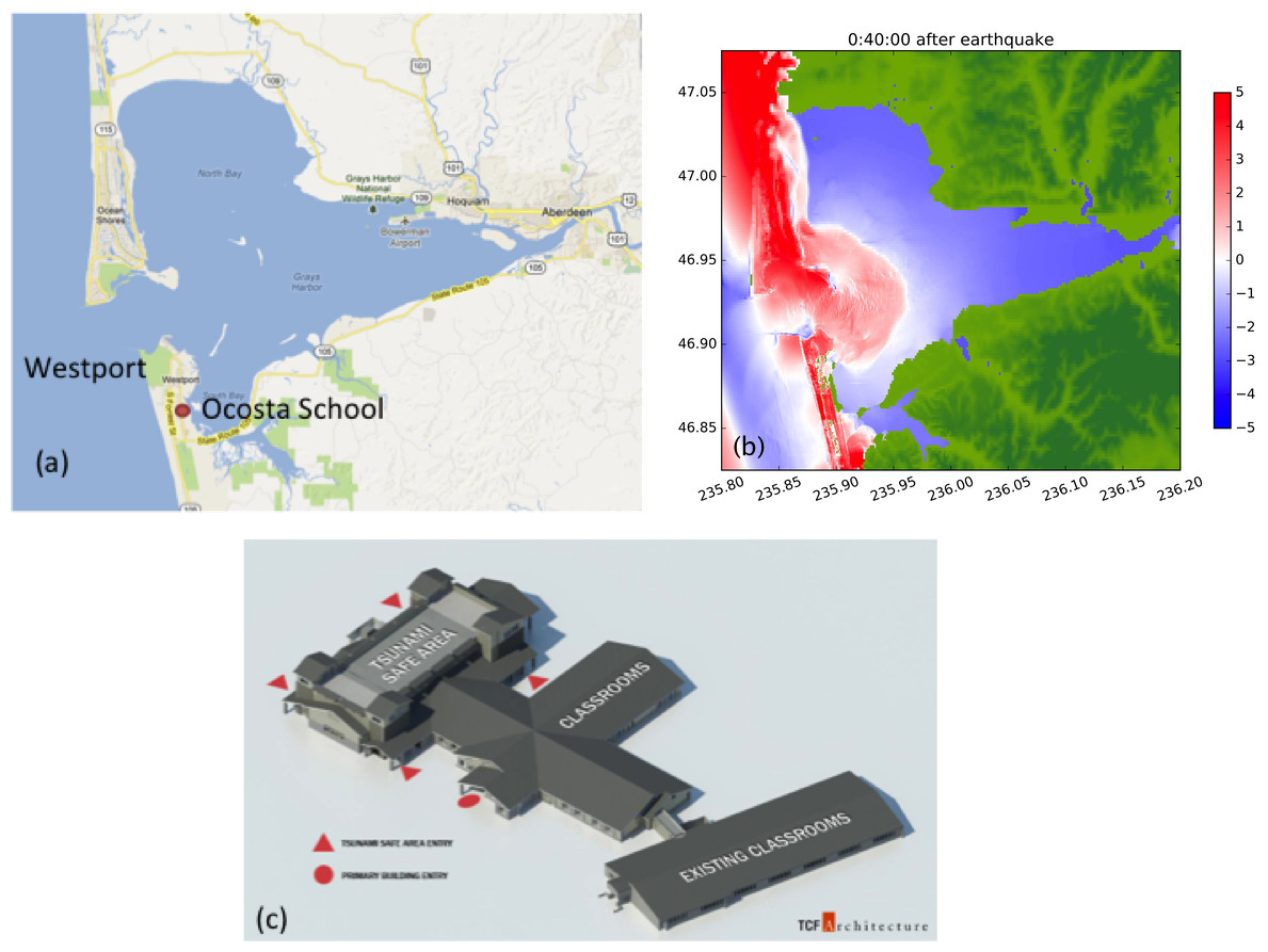
Figure 4: Tsunami Simulation and Planning for Westport, WA.
Gray’s Harbor showing Westport, WA on southern peninsula. (Map data ©2016 Google) (B) Simulation of a potential magnitude 9 Cascadia Subduction Zone event, 40 min after the earthquake. (C) Design for new Ocosta Elementary School in Westport, based in part on GeoClaw simulations (González, LeVeque & Adams, 2013). Image courtesy of TCF Architecture.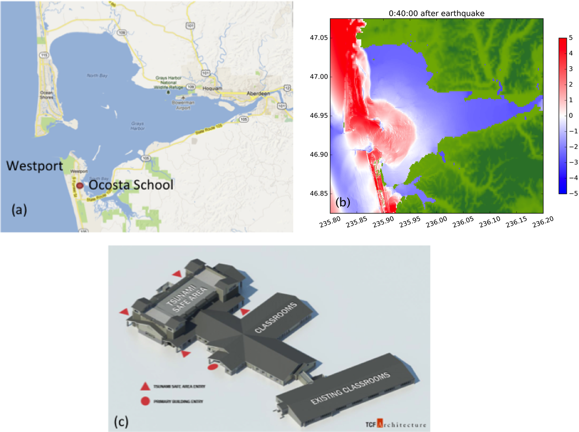
In addition to a variety of tsunami modeling applications, GeoClaw has been used to solve dam break problems in steep terrain (George, 2011), storm surge problems (Mandli & Dawson, 2014) (see Fig. 5 and Table 1), and submarine landslides (Kim, 2014). The code also formed the basis for solving the multi-layer shallow water equations for storm surge modeling (Mandli, 2011; Mandli, 2013), and is currently being extended further to handle debris flow modeling in the packages D-Claw (Iverson & George, 2014; George & Iverson, 2014) (see Figs. 6 and 7).
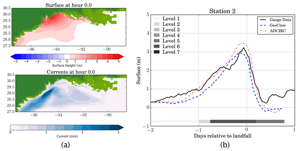
Figure 5: GeoClaw Storm Surge Example.
(A) A snapshot of a GeoClaw storm surge simulation of Hurricane Ike at landfall. (B) Tide gauge data computed from GeoClaw and adcirc along with observed data at the same location.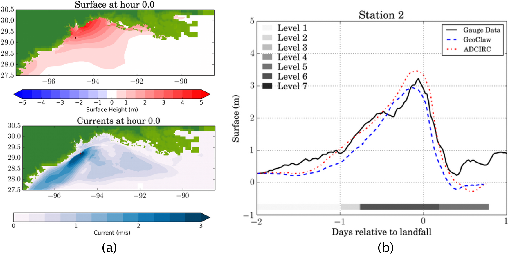
| Package | Threads | Wall Time | Core Time |
|---|---|---|---|
| ADCIRC | 4,000 | 35 min | 2,333 h |
| GeoClaw | 4 | 2 h | 8 h |
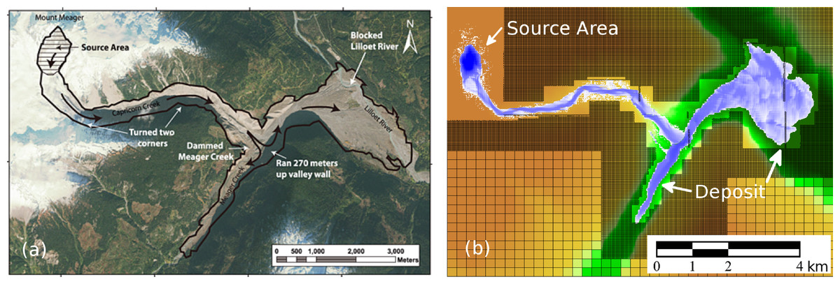
Figure 6: Debris-Flow Examples.
(A) Photograph of the 2010 Mt. Meager debris-flow deposit, from Allstadt (2013). (B) Simulated debris flow, from D. George.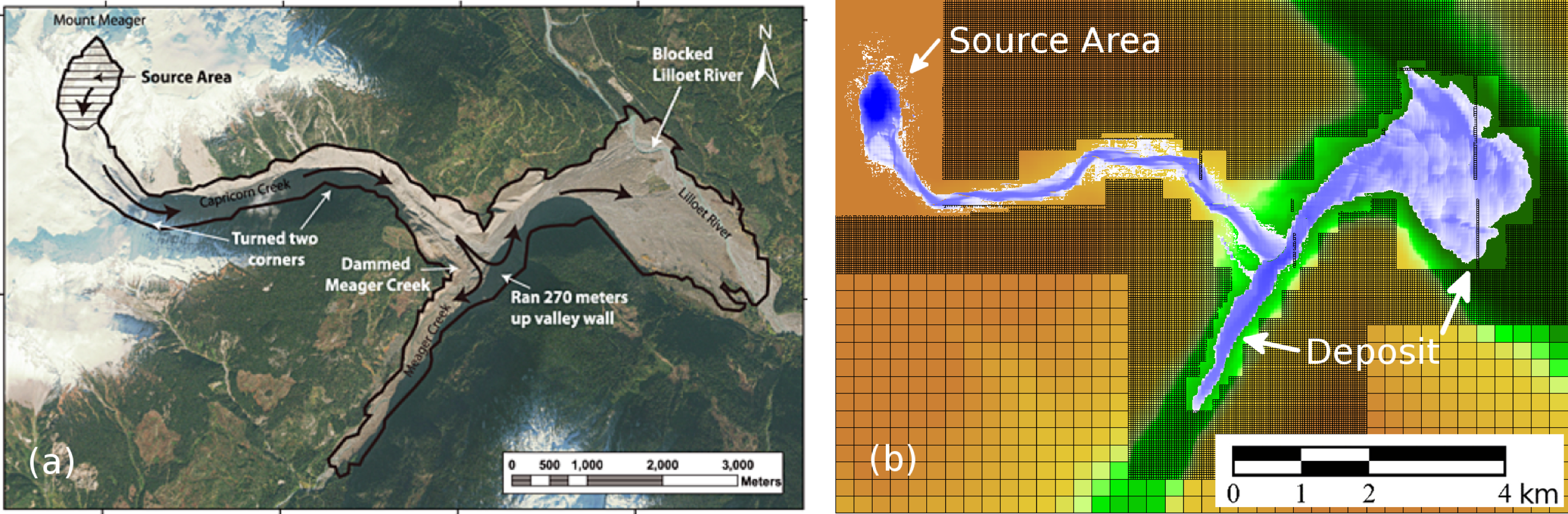
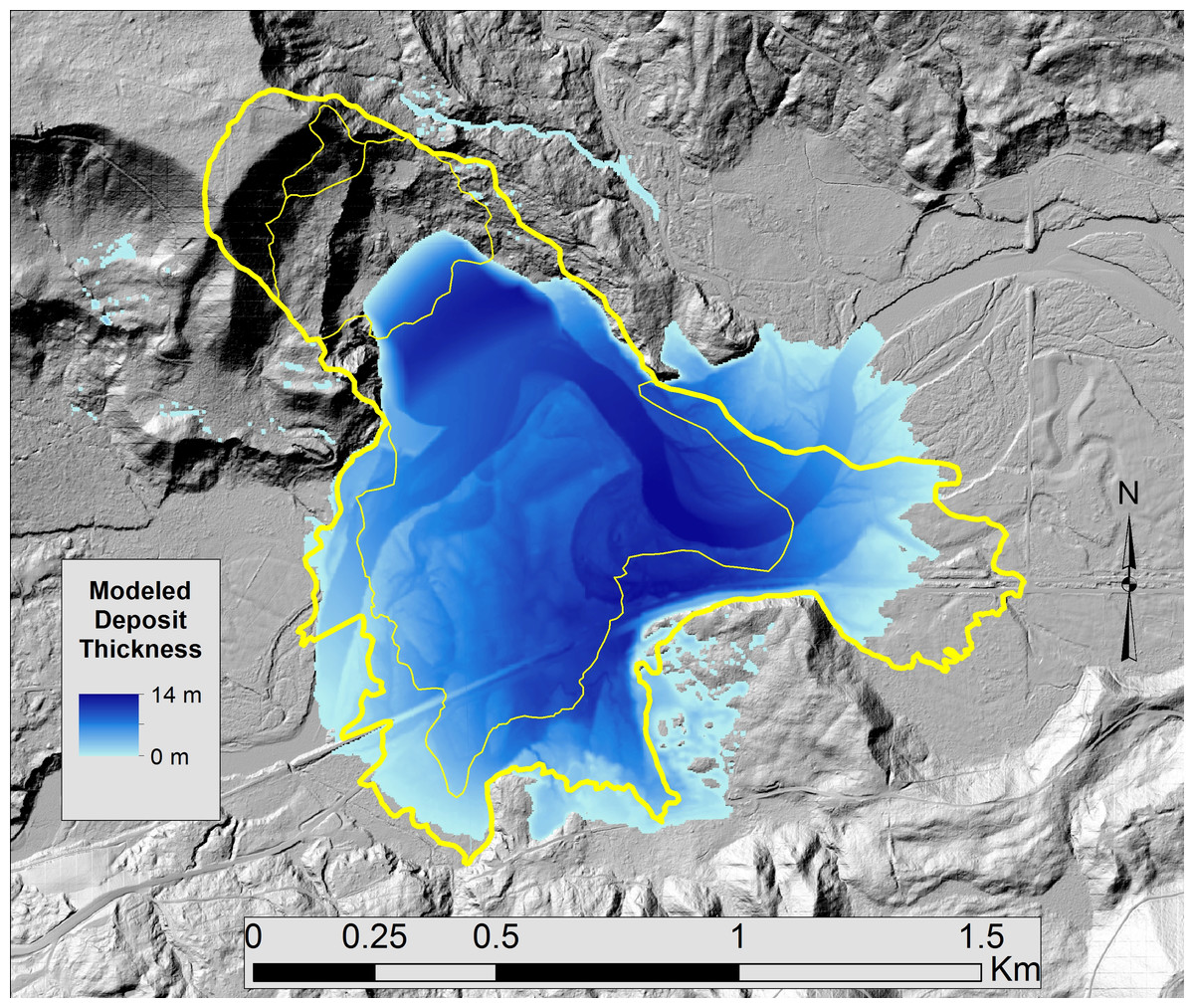
Figure 7: Oso, WA Landslide Simulation.
Observed (yellow line) and computed (blue) landslide at Oso, WA in 2014 (Iverson et al., 2015).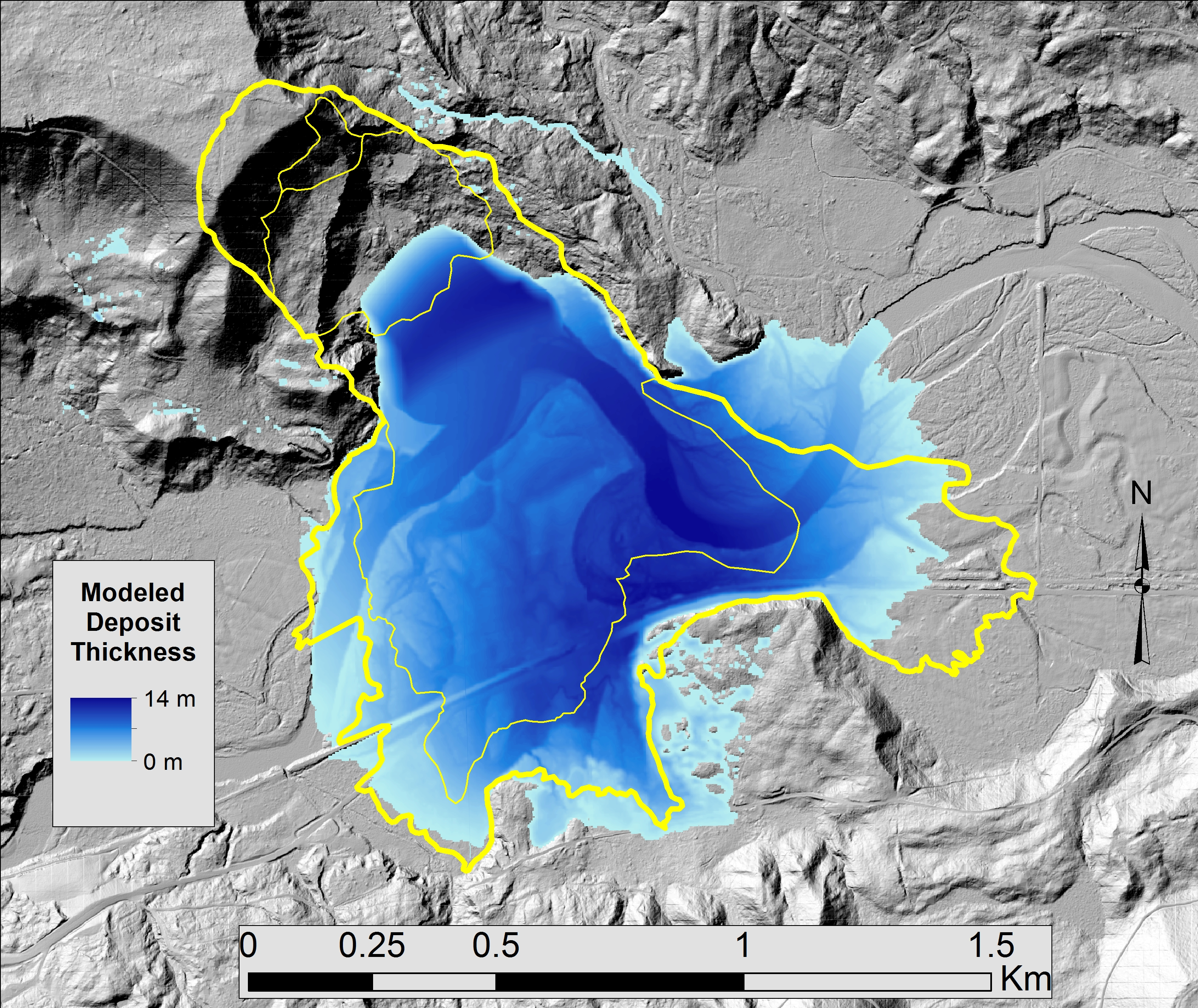
Nearly one quarter of the files in the AMRClaw source library have to be modified for GeoClaw. There are currently 113 files in the AMRClaw 2D library, of which 26 are replaced by a GeoClaw-specific files of the same name in the GeoClaw 2D library. For example, to preserve a flat sea surface when interpolating, it is necessary to interpolate the surface elevation (topography plus water depth) rather than simply interpolating the depth component of the solution vector as would normally be done in AMRClaw. An additional 24 files in the GeoClaw shallow water equations library handle other complications introduced by the need to model tsunamis and storm surge.
Several other substantial improvements in the algorithms implemented in GeoClaw have been made between versions 4.6 and 5.3.0, including:
-
In depth-averaged flow, the wave speed and therefore the CFL condition depends on the depth. As a result, flows in shallow water that have been refined spatially may not need to be refined in time. This “variable-time-stepping” was easily added along with the anisotropic capabilities that were added to AMRClaw.
-
The ability to specify topography via a set of topo files that may cover overlapping regions at different resolutions has been added. The finite volume method requires cell averages of topography, computed by integrating a piecewise bilinear function constructed from the input topo files over each grid cell. In Clawpack 5.1.0, this was improved to allow an arbitrary number of nested topo grids. When adaptive mesh refinement is used, regridding may take place every few time steps. Improvements were made in 5.2.0 so that topography could be copied rather than always being recomputed in regions where there is an existing old grid.
-
The user can now provide multiple dtopo files that specify changes to the initial topography at a series of times. This is used to specify sea-floor motion during a tsunamigenic earthquake, but can also be used to specify submarine landslide motion or a failing dam, for example.
-
A number of new Python modules has been developed to assist the user in working with topo and dtopo files. These are documented in the Clawpack documentation and several of them are illustrated with Jupyter notebooks found in the Clawpack Gallery.
-
New capabilities were added in 5.0.0 to monitor the maximum of various flow quantities over a specified time range of a simulation. This capability is crucial for many applications where the maximum flow depth at each point, maximum current velocities in a harbor, or maximum momentum flux (a measure of the hydrodynamic force that would be exerted by the flow on a structure) is desired. Arrival time of the first wave at each point can also be monitored. Such capabilities were included in the 4.x version of the code, but were more limited and did not always perform properly near the edges of refinement patches. In Version 5.2 these routines were further improved and extended. The user can specify a grid of points on which to monitor values, and the new code is more flexible in allowing one-dimensional grids (e.g., a transect), two-dimensional rectangular grids, or an arbitrary set of points.3
PyClaw
PyClaw is an object-oriented Python package that provides a convenient way to set up problems and call the algorithms of Clawpack. It grew from what was initially a set of data structures and file IO routines that are used by the other Clawpack codes and by VisClaw. These routines were released in an early form in later 4.x versions of Clawpack. Those releases also included a fully-functional implementation of the 1D classic algorithm in pure Python. That implementation still exists in PyClaw and is useful for understanding the algorithm.
The current release of PyClaw includes access to the classic algorithms as well as the high-order algorithms introduced in SharpClaw (Ketcheson, Parsani & LeVeque, 2013) (i.e., WENO reconstruction and Runge–Kutta integrators) and can be used on large distributed-memory parallel machines. For the latter capability, PyClaw relies on PETSc (Balay et al., 2010). Lower-level code (whatever gets executed repeatedly and needs to be fast) from the earlier Fortran Classic and SharpClaw codes is automatically wrapped at install time using f2py.
Recent applications of PyClaw include studies of laser light trapping by moving refractive index perturbations (San Roman Alerigi, 2015), instabilities of weakly nonlinear detonation waves (Faria & Kasimov, 2015), and effective dispersion of nonlinear waves via diffraction in periodic materials (Ketcheson & Quezada de Luna, 2015). Two of these are depicted in Fig. 8.
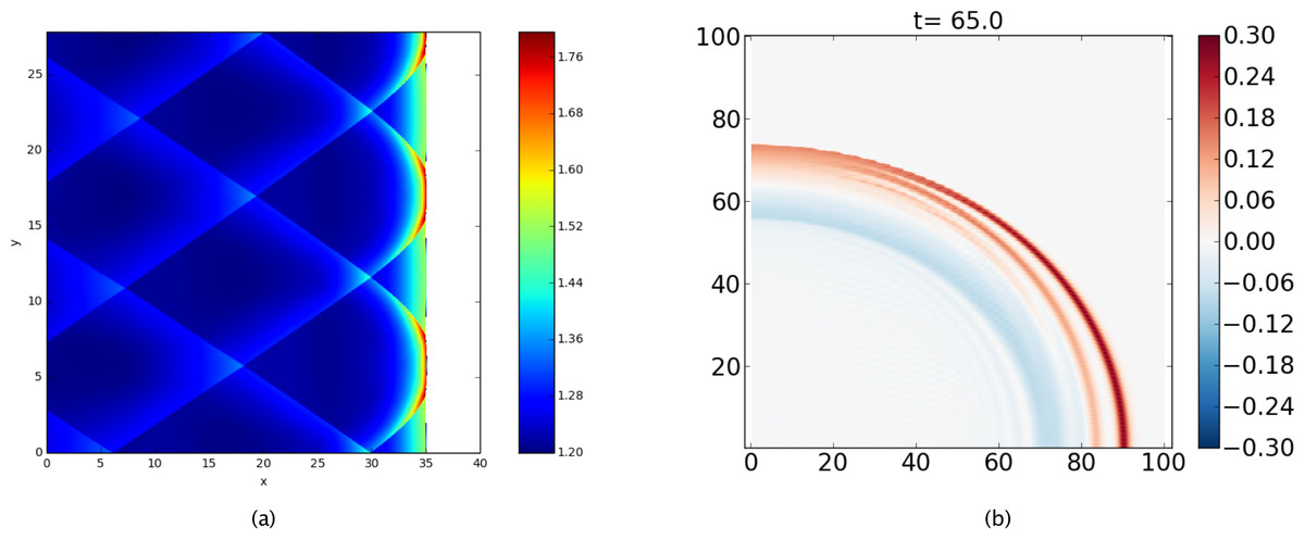
Figure 8: PyClaw Example Simulations.
(A) A two-dimensional detonation wave solution of the reactive Euler equations, showing transverse shocks that arise from instabilities; see Faria & Kasimov (2015). (B) Dispersion of waves in a layered medium with matched impedance and periodically-varying sound speed; see Ketcheson & Quezada de Luna (2015).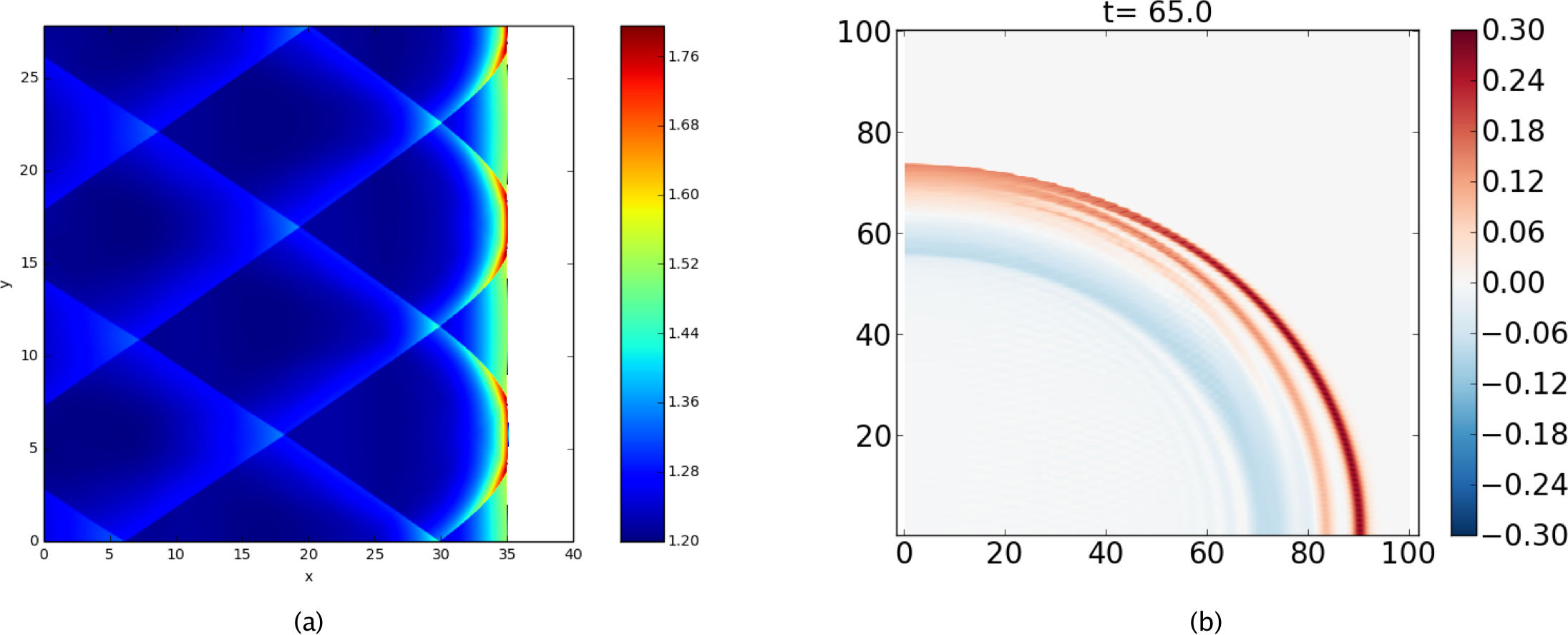
Librarization and extensibility
Scientific software is easier to use, extend, and integrate with other tools when it is designed as a library (Brown, Knepley & Smith, 2015). Clawpack has always been designed to be extensible, but PyClaw takes this further in several ways. First, it is distributed via a widely-used package management system, pip. Second, the default installation process (“pip install clawpack”) provides the user with a fully-compiled code and does not require setting environment variables. Like other Clawpack packages, PyClaw provides several “hooks” for users to plug in custom routines (for instance, to specify boundary conditions). In PyClaw, these routines –including the Riemann solver itself –are selected at run-time, rather than at compile-time. These routines can be written directly in Python, or (if they are performance-critical) in a compiled language (like Fortran or C) and wrapped with one of the many available tools. Problem setup (including things like initial conditions, algorithm selection, and output specification) is also performed at run-time, which means that researchers can bypass much of the slower code-compile-execute-post-process cycle. It is intended that PyClaw be easily usable within other packages (without control of main()).
Python geometry
PyClaw includes Python classes for describing collections of structured grids and data on them. These classes are also used by the other codes and VisClaw, for post-processing. A mesh in Clawpack always consists of a set of (possibly mapped) tensor-product grids (interval, quadrilateral, or hexahedral), also referred to as patches. At present, PyClaw solvers operate only on a single patch, but the geometry and grids already incorporate multi-patch capabilities for visualization in AMRClaw and GeoClaw.
PyClaw solvers
PyClaw includes an interface to both the Classic solvers (already described above) and those of SharpClaw (Ketcheson et al., 2012). SharpClaw uses a traditional method-of-lines approach to achieve high-order resolution in space and time. Spatial operators are discretized first, resulting in a system of ODEs that is then solved using Runge–Kutta or linear multistep methods. The spatial derivatives are computed using a weighted essentially non-oscillatory (WENO) reconstruction from cell averages, which suppresses spurious oscillations near discontinuities. The WENO routines in SharpClaw were generated by PyWENO (http://github.com/memmett/PyWENO), which is a standalone package that generates WENO routines.
The default time stepping routines in SharpClaw are strong stability preserving (SSP) Runge–Kutta methods of order two to four. Some of the methods use extra stages in order to allow more efficient time stepping with larger CFL numbers. Time stepping in SharpClaw has recently been augmented to include linear multistep methods with variable step size. These methods use a time step size selection that ensures the strong stability preserving property, as described in Hadjimichael et al. (2016).
Parallelism
PyClaw includes a distributed parallel backend that uses PETSc through the Python wrapper petsc4py. The parallel code uses the same low-level routines without modification. In the high-level routines, only a few hundred lines of Python code deal explicitly with parallel communication, in order to transfer ghost cell information between subdomains and to find the global maximum CFL number in order to adapt the time step size. For instance, the computation shown in the right part of Fig. 8 involved more than 120 million degrees of freedom and was run on two racks of the Shaheen I BlueGene/P supercomputer. The code has been demonstrated to scale with better than 90% efficiency in even larger tests on tens of thousands of processors on both the Shaheen I (BlueGene/P) and Shaheen II (Cray XC40) supercomputers at KAUST. A hybrid MPI/OpenMP version is already available in a development branch and will be included in future releases.
VisClaw : visualizing Clawpack output
A practical way to visualize the results of simulations is essential to any software package for solving PDEs. This is particularly true for simulations making use of adaptive mesh refinement, since most available visualization packages do not have tools that conveniently visualize hierarchical AMR data. VisClaw provides support for all of the main Clawpack submodules, including ClassicClaw, AMRClaw, PyClaw and GeoClaw.
From the first release in 1994, Clawpack has included tools for visualizing the output of Clawpack and AMRClaw runs. Up until the release of version Clawpack 4.x, these visualization tools consisted primarily of Matlab routines for creating one, two and three dimensional plots including pseudo-color plots, Schlieren plots, contour plots and scatter plots, including radially or spherically symmetric data. Built-in tools were also available for handling one, two and three-dimensional mapped grids. Starting with version 4.x, however, it was recognized that a reliance on proprietary software for visualization prevented a sizable potential user base from making use of the Clawpack software. The one and two dimensional plotting routines were converted from Matlab to matplotlib, a popular open source Python package for producing publication quality graphics for one and two dimensional data (Hunter, 2007).
With the development of Clawpack Version 5 and above, Python graphics tools have been collected into the VisClaw repository. The VisClaw tools extend the functionality of the Version 4.x Python routines for creating one and two dimensional plots, and adds several new capabilities. Chief among these are the ability to generate output to webpages, where a series of plots can be viewed individually or as an animated time sequence using the Javascript package (https://github.com/jakevdp/JSAnimation) (which was motivated by code in an earlier version of Clawpack). The VisClaw module Iplotclaw provides interactive plotting capabilities from the Python or IPython prompt. Providing much of the same interactive capabilities as the original Matlab routines, Iplotclaw allows the user to step, interactively, through a time sequence of plots, jump from one frame to another, or interactively explore data from the current time frame.
Tools for visualizing geo-spatial data produced by GeoClaw
The geo-spatial data generated by GeoClaw has particular visualization requirements. Tsunami or storm surge simulations are most useful when the plots showing inundation or flooding levels are overlaid onto background bathymetry or topography. Supplementary one dimensional time series data (e.g., gauge data) numerically interpolated from the simulation at fixed spatial locations are most useful when compared graphically to observational data. Finally, to more thoroughly analyze the computational data, simulation data should be made available in formats that can be easily exported to GIS tools such as ArcGIS (http://www.arcgis.com) or the open source alternative QGIS (http://www.qgis.org). For exploration of preliminary results or communicating results to non-experts, Google Earth is also helpful.
The latest release of Clawpack includes many specialized VisClaw routines for handling the above issues with plotting geo-spatial data. Topography or bathymetry data that was used in the simulation will be read by the graphing routines, and, using distinct colormaps, both water and land can be viewed on the same plot. Additionally, gauge locations can be added, along with contours of water and land. One dimensional gauge plots are also created, according to user-customizable routines. In these gauge plotting routines, users can easily include observational data to compare with GeoClaw simulation results.
In addition to HTML and Latex formats available for all Clawpack results, VisClaw will now also produce KML and KMZ files suitable for visualizing results in Google Earth. Using the same matplotlib graphics routines, VisClaw creates PNG files that can be used as GroundOverlay features in a KML file. Other features, such as gauges, borders on AMR grids, and user specified regions can also be shown on Google Earth. All KML and PNG files are compressed into a single KMZ file that can be opened directly in Google Earth or made available online. While VisClaw does not have any direct support for ArcGIS or QGIS, the KML files created for Google Earth can be edited for export, along with associated PNG files to these other GIS applications.
Matlab plotting routines
The Matlab plotting tools available in early versions of Clawpack are still included in VisClaw. While most of the one and two dimensional capabilities available originally in the Matlab suite have been ported to Python and matplotlib, the original Matlab routines are still available in the Matlab suite of plotting tools. Other plotting capabilities, such as two dimensional manifolds embedded in three dimensional space, or three dimensional plots of fully three-dimensional data are only available in the Matlab routines in a way that interfaces directly with Clawpack. More advanced three-dimensional plotting capabilities are planned for future releases of VisClaw.
Conclusions
Clawpack has evolved over the past 20 years from its genesis as a small and focused software package that two core developers could manage without version control. It is now an ecosystem of related projects that share a core philosophy and some common code (notably Riemann solvers and visualization tools), but that are aimed at different user communities and that are developed by overlapping but somewhat distinct groups of developers scattered at many institutions. The adoption of better software engineering practices, in particular the use of Git and GitHub as an open development platform and the use of pull requests to discuss proposed changes, has been instrumental in facilitating the development of many of the new capabilities summarized in this paper. These developer facing improvements of course affect the user as well since better and faster development cycles means better and faster implementation of features. The user facing features already implemented in version 5 have opened up the use of Clawpack to a broader audience.
Future plans
The Clawpack development team continues to look forward to new ideas and efforts that will allow great accessibility to the project as well as new capabilities that the core development team has not thought of. To this end a number of the broad efforts that are being considered for the next major release of Clawpack include
-
An increased librarization effort with the Fortran based sub-packages,
-
An extensible and more accessible interface to the Riemann solvers,
-
An effort to allow PyClaw and the Clawpack Fortran packages to rely on more of the same code-base,
-
An increased emphasis on a larger development community,
-
More support for new frameworks such as ForestClaw (Burstedde et al., 2014),
-
Adjoint error estimation for flagging cells to increase the efficiency of the AMR codes (Davis & LeVeque, 2015),
-
A refactoring of the visualization tools in VisClaw, along with support for additional backends, particularly for three-dimensional results (e.g., Mayavi (http://docs.enthought.com/mayavi/mayavi/), VisIt (https://visit.llnl.gov), ParaView (http://www.paraview.org/), or yt (http://yt-project.org/)).