
Efficient online detection of temporal patterns
- Published
- Accepted
- Received
- Academic Editor
- Mohammad Reza Mousavi
- Subject Areas
- Algorithms and Analysis of Algorithms, Theory and Formal Methods
- Keywords
- Pattern matching, Verification, Time series
- Copyright
- © 2016 Dolev et al.
- Licence
- This is an open access article distributed under the terms of the Creative Commons Attribution License, which permits unrestricted use, distribution, reproduction and adaptation in any medium and for any purpose provided that it is properly attributed. For attribution, the original author(s), title, publication source (PeerJ Computer Science) and either DOI or URL of the article must be cited.
- Cite this article
- 2016. Efficient online detection of temporal patterns. PeerJ Computer Science 2:e53 https://doi.org/10.7717/peerj-cs.53
Abstract
Identifying a temporal pattern of events is a fundamental task of online (real-time) verification. We present efficient schemes for online monitoring of events for identifying desired/undesired patterns of events. The schemes use preprocessing to ensure that the number of comparisons during run-time is minimized. In particular, the first comparison following the time point when an execution sub-sequence cannot be further extended to satisfy the temporal requirements halts the process that monitors the sub-sequence.
Introduction
Many complex systems, both hardware and software, require sound verification of their operation, usually in the form of safety and liveness properties. One of the prominent formal verification methods used today is model checking, which models the system as a state-transition system, and performs an exhaustive search of its state-transition graph for possible runs where desired properties do not hold. In model checking, a precise description of the system to check is mandatory as, before actually running the system, all possible executions must be checked (Bauer, Leucker & Schallhart, 2011). One of the drawbacks of model checking is the state explosion problem (Rafe, Rahmani & Rashidi, 2013): explosion due to the need to explore an exponential number of states which grow with relation to the number of system variables. This yields a costly check. Another significant problem is in the modeling process itself. The verification is only as good as the model of the (actual hardware and software) implementation rather than the implementation itself. Online model checking is presented as a lightweight verification technique to overcome the state space explosion problem. However, the computational complexity of the proposed online model checking in time and space is less than that of (off-line) model checking, but greater than that of runtime verification (Zhao & Rammig, 2012).
An even older classical method to verify system specifications is testing (Luo, 0000). While testing examines the implemented system (rather than only a model of the system), it is impossible for complex systems because the number of input sequences grow exponentially with the given sequence length. Of course, an exhaustive search for specification violations is not feasible. Thus, runtime verification may assist in coping with implementation flaws that materialize only during (specific, rare) executions. Runtime verification has been developed to check for desired properties at runtime on the active execution path. System properties are written in a formal logic and then transformed into a runtime monitor (Colombo, Pace & Schneider, 2008). The transformations from design models to implementation are generally informal, therefore error-prone. Runtime verification validates transformations indirectly and provides a mechanism to handle exceptions of implementations that are not detected during development or testing (Dong et al., 2005).
We concentrated on a specific task of runtime verification; namely, the detection of temporal patterns. Rather than modeling the system and searching its entire state-transition graph, as is done in model checking, we devised an approach toward verification of time restrictions over sequences of events at system runtime. We used temporal constraint semantics to describe the specification.
Our contribution. We designed several algorithms which, given a description of the system as a set of possible events and a specification of safety properties as desired/undesired temporal patterns, monitor the system and detect when such patterns occur. We distinguished between several scenarios depending on the pattern profile: sporadic/continuous patterns, max-/max and min- constrained patterns.
First, we describe how to preprocess the input patterns in graph form to get their minimized representation by removing redundant constraints. Then, we describe an automaton which tracks pattern prefixes using tokens and detects pattern completion. This automaton tracks the system events efficiently. Once a token does not adhere to some temporal constraint, the token is discarded within one comparison; this is in addition an earliest possible notification on when a completed pattern is given.
Related work. Runtime verification is being pursued as a lightweight verification technique complementing verification techniques such as model checking and testing and establishes another trade-off point between these forces. One of the main distinguishing features of runtime verification is due to its nature of being performed at runtime, which opens up the possibility to act whenever incorrect software system behavior is detected (Leucker & Schallhart, 2009).
Runtime verification of asynchronous systems for ensuring safety and liveness specifications by monitoring events has been discussed in e.g., Dolev & Stomp (2003); Brukman & Dolev (2006); Brukman, Dolev & Kolodner (2008); Brukman & Dolev (2008). A parametric real-time monitoring system with multiple logical structures is proposed in Jin et al. (2012). Dynamic communicating automata with timers and events to describe properties of systems which need to be checked for different instances online are introduced in Colombo, Pace & Schneider (2008). However, the implementation overhead is very high to implement this method.
In contrast, we are interested in monitoring timed events in synchronous (or semi-synchronous real-time) systems. The preprocessing phase resembles results in Temporal Constraint Networks (Dechter, Meiri & Pearl, 1991). In contrast, Dechter, Meiri & Pearl (1991) does not consider the on-line monitoring task and its composition with the preprocessing phase. In order to detect desired/undesired patterns of events we employ methods similar to classical string matching solutions (Crochemore, 1988), though in our scope, system events must occur in a timely manner to fit a given pattern.
A fundamental discussion of model checking appears in Clarke, Grumberg & Peled (1999), and a popular method to address the state explosion problem (Groote, Kouters & Osaiweran, 2012) of model checking is described in Burch et al. (1992), by representing the state transition graph using propositional logic formulae. Zhao & Rammig (2012) discusses a special form of online model checking method for runtime verification, which provide the model and implementation of the system to verify. A temporal logic is proposed in Baldan et al. (2006) to specify and verify properties on graph transformation systems. An approach of extending Computation Tree Logic(CTL) to include timing constraints appears in Alur, Courcoubetis & Dill (1993). In Laroussinie, Markey & Schnoebelen (2006), transitional durations are added to timed temporal formulae as an extension of Kripke Structures, and timed versions of CTL are considered. These frameworks however, do not address real-time verification.
Linear Temporal logic (LTL) has been used for runtime verification; however, it is best suited for design-time system verification. Also, the evaluation of LTL properties on finite traces proved to be an obstacle, as LTL is usually evaluated over infinite traces. The standard semantics of LTL on finite traces is unsatisfactory for the purpose at hand (Andreas, Martin & Christian, 2010).
Tools for real-time verification exist in the form of assertion checking, some of which follow the PSL IEEE standard, notably Colombo, Pace & Schneider (2008); Alur, Courcoubetis & Dill (1993); Brukman, Dolev & Kolodner (2008); further comparison of these tools is beyond the scope of this article. While these allow the specification of quite general properties and employ an automaton for detecting a single property, we focus on patterns with timing constraints and employ an automaton to detect all pattern instances.
Model programs have been rarely used for runtime verification (see Blum & Wasserman, (1997) for example). As long as model programs are deterministic and contain no mandatory calls, they can be verified easily. But, for the model programs containing non-deterministic expressions or mandatory calls, we need tighter integration (Barnett & Schulte, 2003).
Organization. The formal setting is presented in the next section, along with detection of continuous temporal patterns. In ‘Sporadic Pattern Match,’ we study the less restricted definition of sporadic temporal patterns by analyzing the pattern’s temporal constraints, semantics, and devise a detection algorithm. Next, we briefly discuss an approach for estimating the probability of a partial pattern match completing a full pattern match in ‘Prediction and Alert of a Near Pattern Match.’ Finally, concluding remarks and future research scope appear in ‘Concluding Remarks.’
Continuous Pattern Match
An event type a is a discrete input to our system taken from a given set of possible inputs, called the event type set. A timed event, te, is a tuple (a, t) such that a is an event type and t is the time at which type a event took place. Similar to multi-event segments in simulation theory (Zeigler, Kim & Praehofer, 2000), we define an execution of a system as an input stream of timed events te1 = (a1, t1), te2 = (a2, t2), …, such that for every two timed events tei and tei+1 it holds that ti < ti+1. We assume that events in the system occur in discrete time points (over ).
A temporal pattern TP is a tuple (A, C), where A = (a1, a2, …, an) is a sequence of typed (non-timed) events. Each ai has a type ai.type from the event type set. Event types are not necessarily distinct: C is a set of temporal constraints, such that each c ∈ C is a tuple (ai, aj, w), where the time interval between the events ai and aj is at most w. We call such a constraint a max constraint; in ‘Adding minimum constraints’ we will address min constraints.
Detection of continuous temporal patterns. We track a stream of timed events to identify temporal patterns that respect the constraints of TP. We consider the simple case of a continuous pattern. For every 1 < i < n − 1, we call ai and ai+1 consecutive events. A continuous pattern match is an execution sub-sequence where consecutive events happen successively. A (type-wise)1 execution a1, …, ai, b, ai+2, …, an where b.type ≠ ai+1.type is not considered a match.
Directed graphs and tokens. A temporal pattern (A, C) is represented by a pattern graph. The events in A define the graph nodes, and the constraints in C define edges. A constraint e = (ai, aj, w) where i < j is a directed edge from ai to aj with weight w. We denote ai and aj by e.src and e.dst, respectively. If there is no constraint between ai and ai+1 for some i, we define an edge (ai, ai+1, ∞), where ∞ signifies that any finite time may pass between ai and ai+1. An edge between consecutive events is a simple edge, and any other edge is an overpassing edge. A path using only simple edges is a simple path. (a1, a2, …, an) is defined as the chronological order of the pattern’s events. In particular, G is a WDAG (Weighted DAG).
A preprocessing phase of pattern constraints is explained in ‘Sporadic Pattern Match.’
Execution sub-sequences that partially match a pattern are represented by tokens. A token resides on an event, and carries with it a history of the time points at which it reached previous events. HandleEvent (Alg. 1) handles an event log received from the system in the form of a timed event (type, t), where type is the event type and t is the time point at which it occurred. If tkn is a token currently residing on the graph, then tkn.evnt and tkn.h are the events on which the token resides, and the token’s history, respectively. The method getTime(a) of tkn.h returns the time point at which tkn reached a.
   1  tkns := set of graph tokens;
   2  ForEach tkn in tkns Do
   3     b := successor of tkn.evnt;
   4     If (b.type) != type Then discard tkn;
   5     ForEach graph edge (a,b) Do
   6        If (t - tkn.h.getTime(a) > w(a,b))
   7           Then discard tkn;
   8     add (b,t) to tkn.h;
   9     tkn.evnt := b;
   10    If (tkn.evnt is the last event) Then
   11       report tkn;
   12       discard tkn;
   13  If (type matches the first event)
   14     Then add a new token;

    Alg. 1: HandleEvent(type,t)
In (line 1) we receive the set of graph tokens. We handle each such token (line 2). In (line 3) we obtain the successive event of tkn.evnt. If the event’s type does not match type (the logged event’s type), we discard tkn (line 4). We check if all edge constraints whose head is b are satisfied; If not, we discard tkn (lines 5–7). If the constraints are satisfied, we update the token’s history and move tkn to the next event (lines 8–9). If tkn reaches the last pattern event, we report the pattern match and provide its history, and then discard tkn (lines 10–12). Finally, if type matches the type of the first pattern event, we create a new token on the first event (lines 13–14).
An illustration of token tracking is shown in Fig. 1.
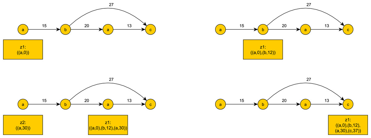
Figure 1: An example of token tracking for the event input stream: ((a, 0), (b, 12), (a, 30), (c, 37)).
z2 becomes obsolete when c occurs. z1 reaches the last event c and completes a continuous pattern match.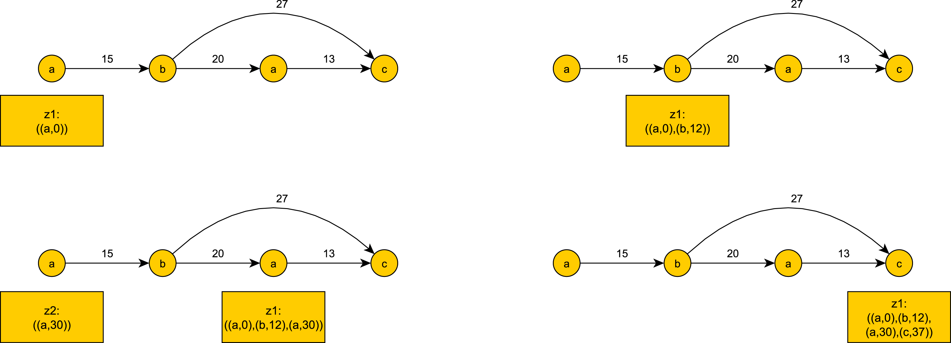
Sporadic Pattern Match
Maximum constraints
A sporadic pattern match is an execution sub-sequence where non-sequential system events may occur between consecutive pattern events. If the temporal pattern events are a1, …, an, a (type-wise) execution a1, …, ai, b, ai+1, …, an where b.type ≠ ai+1.type matches the pattern, as long as the temporal constraints are satisfied. We designed an algorithm to detect sporadic pattern matches, so that a token is discarded at the very first constraint check once it becomes obsolete. We shall describe two phases of the pattern detection paradigm: a preprocessing phase and an on-line detection phase. The preprocessing phase will yield an equivalent temporal pattern in a more restrictive form. The online detection phase will utilize a many-state automaton to keep track of the system’s sub-sequence execution operation, which partially matching a pattern. The sub-sequences are represented by tokens that reside on the automaton’s states.
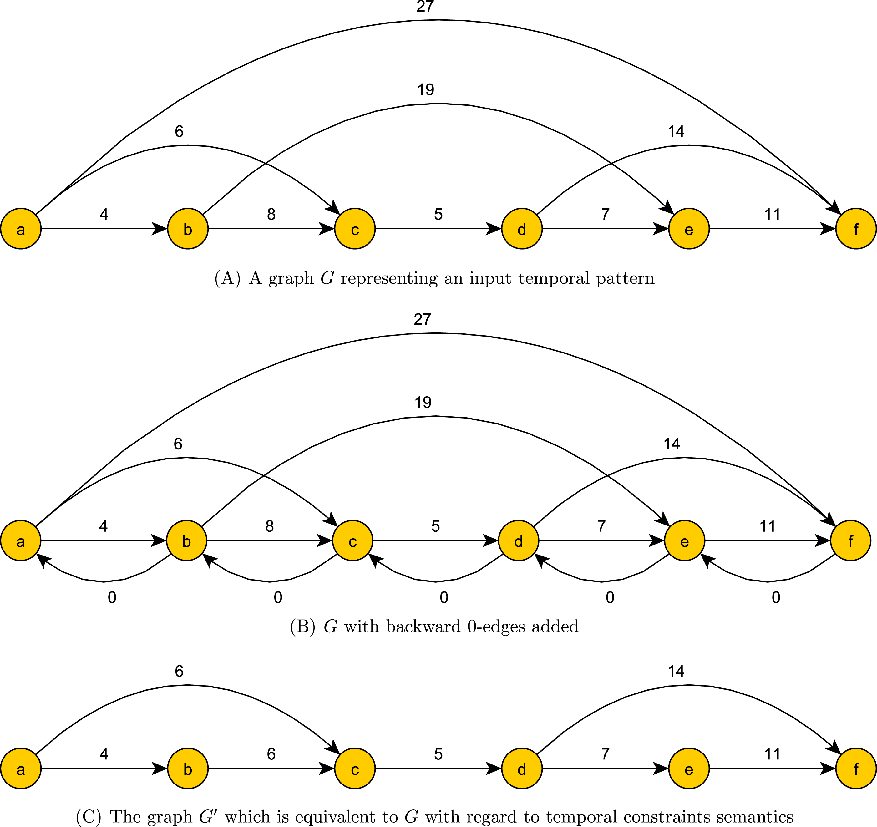
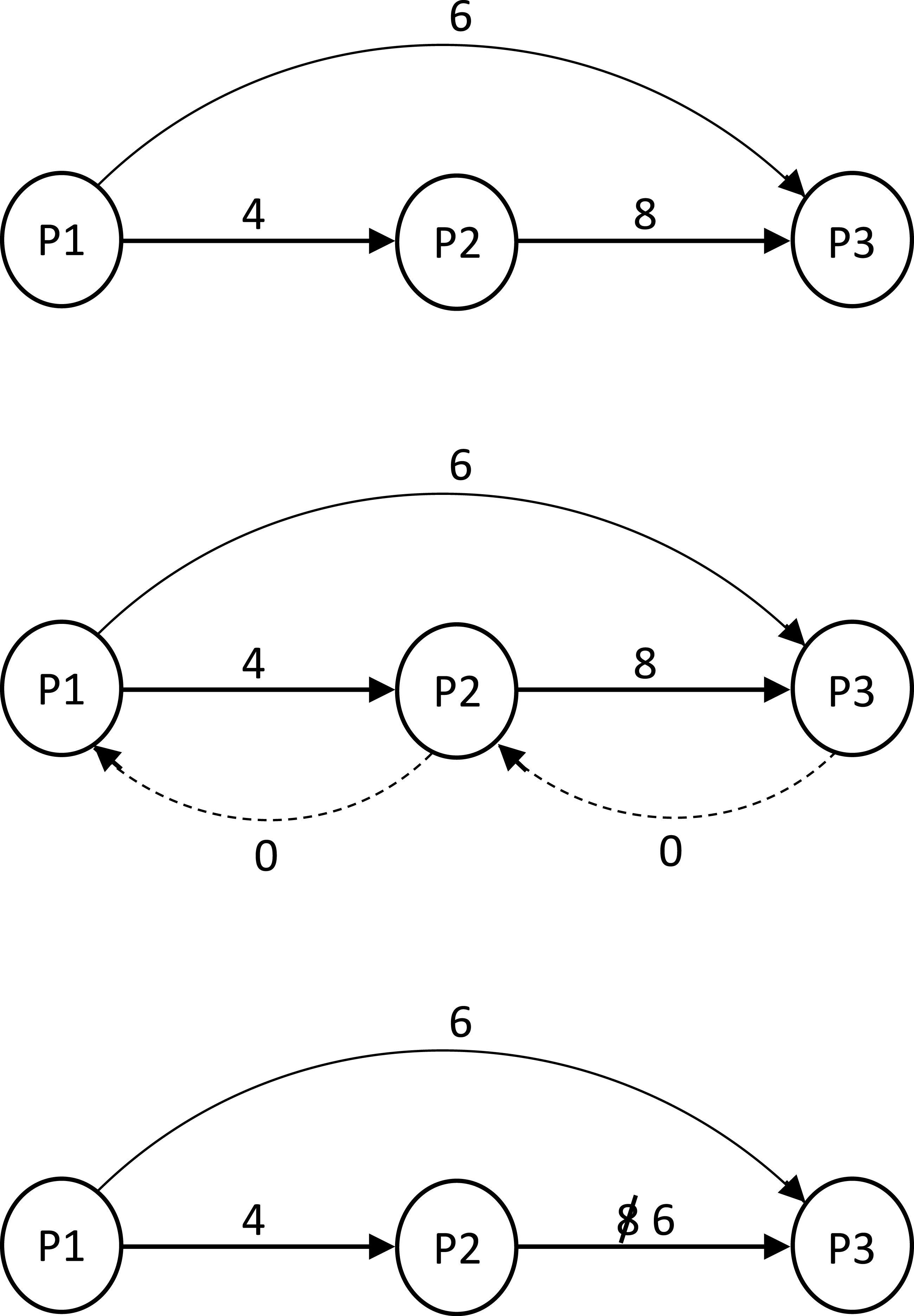
Preprocessing phase. In the preprocessing phase we reduce the pattern constraint set while maintaining the temporal constraint semantics. For every 1 ≤ i < n we add to G an edge (ai+1, ai, 0), which we simply call a 0-edge. We compute the shortest path from ai to aj for 1 < i < n − 1 and i + 1 < j < n. This can be done with O(n3) comparisons using the Floyd–Warshall algorithm. We then update G by removing every overpassing edge that is not the unique shortest path between its ends. In addition, we update the weight of every simple edge to the weight of the shortest path between its ends. This update takes O(n2) comparisons. We denote the ensuing graph modulo the 0-edges as G′. An example of a graph before, during and after preprocessing can be seen in Figs. 2A, 2B and 2C. The role of 0 edges in finding the shortest path between the ends and updating edge weights is illustrated in Fig. 3.
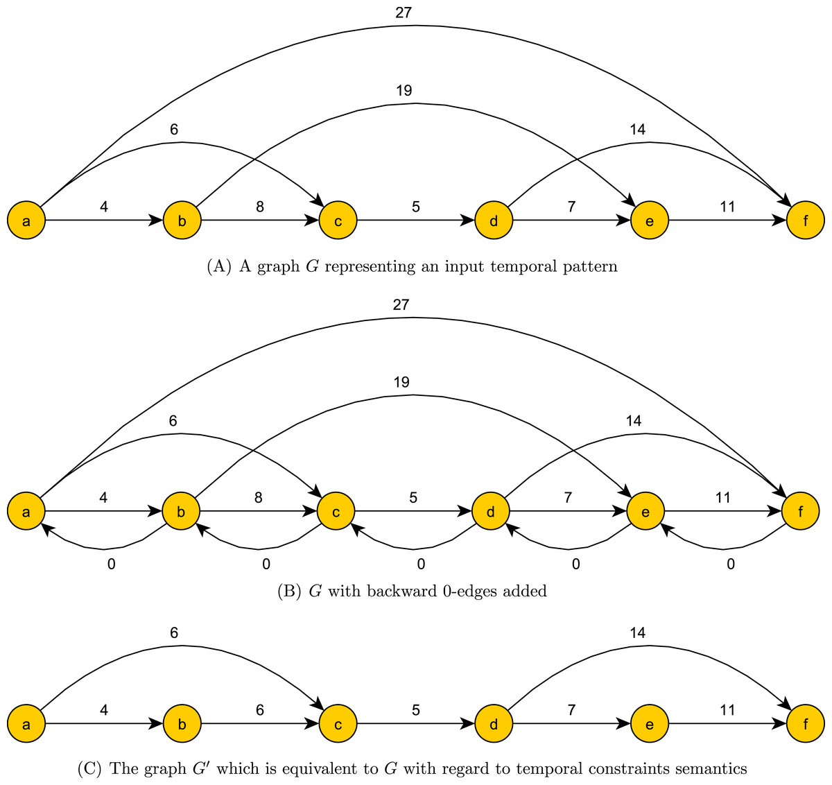
Figure 2: Preprocessing phase of a temporal pattern graph G.
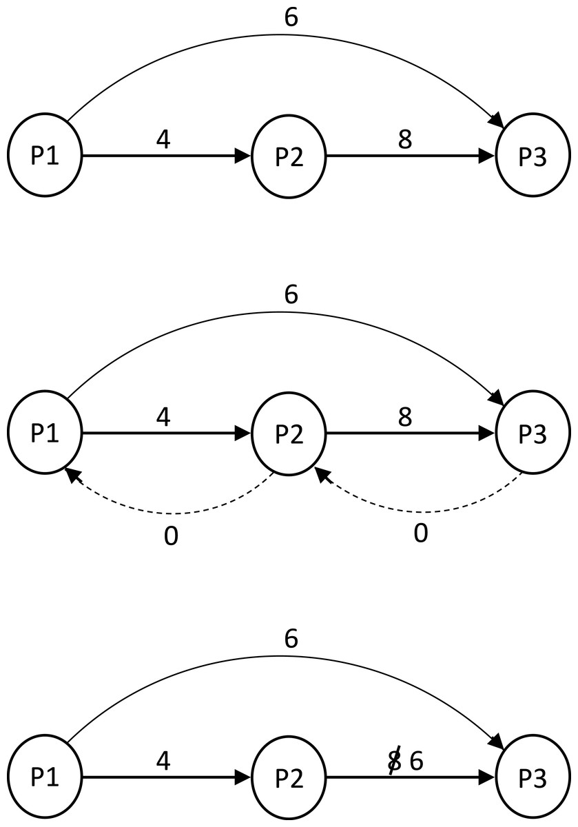
Figure 3: Significance of 0 edges in reducing temporal constraint set.
Histories and graph preorder. We call every single update of G an update step. In the following discussion, the graphs are temporal patterns of n events; the histories consist of these events. A history is a tuple H = ((a1, t1), …, (an, tn)), where tj is the time-point at which aj occurred. We denote tj as H(aj). We denote tj − ti by H(ai, aj) or by H(e), where e = (ai, aj, w) for some w. A history H fits a graph G if: for every (ai, ti) and (aj, tj) in H, if (ai, aj, t) is a weighted edge in G, then H(ai, aj) ≤ t. Alternatively, we say H fits the underlying temporal pattern TP.
We define a preorder ≪ (a reflexive and transitive relation) between graphs as follows: G1 ≪ G2 if for every history H: (H fits G1) implies that (H fits G2). It is easy to show that ≪ is indeed a preorder. ≪ naturally induces an equivalence relation ≡ on graphs: G1 ≡ G2 if G1 ≪ G2 and G2 ≪ G1. In the following discussion, equivalence of graphs refers to the graphs modulo the backward 0-edges.
Let G and G′ be the graphs before and after the execution of preprocessing, respectively. Then the following properties hold:
Equivalence: G ≡ G′.
Minimality: G′ is the minimal graph that is equivalent to G. If any overpassing edge is removed from G′ or if the weight of some edge is reduced in G′, then it will no longer be equivalent to G.
Note that for simplicity we refer to G and G′ as the respective graphs both with and without the 0-edges: with 0-edges when referring to paths, and without 0-edges when referring to history fittings and graph equivalences.
See Appendix S2 for proof. This result is a special case of the results in ‘Adding minimum constraints’ and follows the result in Dechter, Meiri & Pearl (1991).
On-line detection phase. We build an automaton TA whose states are the pattern of events. We may consider the graph as a representation of the automaton, with its events as different states. At any given time in the execution, an event may hold several tokens. A token represents a sub-sequence of the execution, partially matching the temporal pattern. The only transitions are from an event ai to the next event ai+1 for every 1 < i < n − 1, where the rule of the transition is that the token must satisfy the constraint of the simple edge (ai, ai+1). Additionally, a token must satisfy other constraints as explained in the following schemes.
Deadline Scheme. Every token tkn is associated with a minimum heap tkn.DL (for DeadLines) which is empty at first, and with a dynamic hash table tkn.DLH. An element in the heap is a tuple (evnt, dl, ptr), where dl is the deadline for the token to reach the event evnt. If the token does not reach evnt by the time dl, it becomes obsolete. ptr is a pointer to the twin element in tkn.DLH. An element in tkn.DLH is a tuple (evnt, ptr). The event evnt is the key, and ptr is a pointer to the twin element tkn.DL. This duplication of data is necessary to ensure that no more than one instance of some event is in the heap.
    1  tkns := tokens awaiting a type event;
    2  ForEach tkn in tkns Do
    3     m := tkn.DL.min;
    4     If (m.dl < t) Then discard tkn;
    5     b := successor of tkn.evnt;
    6     If b is the last pattern event Then
    7        report matched pattern;
    8        discard tkn;
    9     If (b has a token) Then discard b.tkn;
    10    tkn' := newToken(tkn,b,t)
    11    If (m.evnt=b) Then remove m and m.ptr;
    12    For (e in opEdges(b)) Do
    13       c := e.dst;
    14       If (c is in tkn'.DLH) Then
    15          m0 := tkn'.DLH.get(c).ptr;
    16          If (t+w(e) < m0.dl) Then
    17             m0.dl := t+w(e);
    18             heapify up m0;
    19       Else
    20          m0 := (c,t+w,null);
    21          m1 := (c,m0);
    22          m0.ptr := m1;
    23          insert m0 into tkn.DL;
    24          insert m1 into tkn.DLH;
    25  If (type matches the first event) Then
    26     add new token;

 Alg. 2. HandleEvent(type,t) for Sporadic Pattern Detection
This keeps the space complexity of a token’s heap and hash table to O(n), instead of a possible Θ(n2) for Θ(n2) overpassing edges. tkn.evnt is the event on which tkn exists. We call this scheme the deadline scheme.
If tkn resides on event a and the next chronological event in the pattern b occurs at time t, we first check tkn against the simple edge (a, b). If the constraint does not hold, tkn is discarded from TA. HandleEvent (Alg. 2) handles an event log (type, t). The method newToken(tkn, a, t) spawns a new token a which inherits tkn’s history and adds the element (a, t) to the history of the new token. opEdges(a) returns the set of overpassing edges whose source is a.
In (line 1) we get the tokens awaiting a type event, in descending chronological order. We handle each subsequent token (line 2). In (line 3) we check the minimum element m of tkn.DL. If m.dl < t, tkn is discarded from TA along with its associated data structures, then we check the next token in tkns (line 4). If tkn is valid and the next event is the last pattern event, we report a pattern match and discard tkn (lines 6–8). Otherwise, if b, the next chronological event after tkn.evnt, holds a token, then the old token is discarded (line 9). We spawn a new token tkn′ on b that inherits tkn.DL and tkn.DLH (line 10). If m.evnt = b, we remove m from tkn′.DL and m.ptr from tkn′.DLH (line 11), since this deadline is no longer relevant. Furthermore, every overpassing edge that going from b may contribute a deadline to tkn′.DL: for every overpassing edge e = (b, c, w), we check if the key c appears in tkn′.DLH (line 14). If it appears as (c, ptr1), let ptr1 = m0 = (c, dl, ptr0). If t + w(e) < dl, we change the value of dl to t + w, and then move m0 up the heap until the heap property holds (lines 16–18). If dl ≤ t + w(e), we do nothing. If c does not appear in tkn′.DLH, we create twin elements m0 = (c, t + w, ptr0) and m1 = (c, ptr1), such that ptri points to mi−1, and insert them in tkn.DL and tkn.DLH, respectively (lines 19–24). If type is the first pattern event type, we create a new token with an attached heap and hash table and add the appropriate deadlines (lines 25–26).
We handle the tokens by the events they reside, from late to early. The reason for this is as follows: say we have tokens on events ai and ai+1, and the type of events ai+1 and ai+2 is type, now a type event occurs. If we handle the token on ai first, it will discard the token on ai+1, though that token may spawn a token on ai+2. Thus, we lose a possible pattern match.
The reason we spawn a new token tkn′ on ai+1 rather than moving tkn to ai+1 is that ai+1 may occur again while tkn is still relevant. Thus spawning a new token tkn″ with different deadlines than those of tkn′. This algorithm ensures we detect the first instance of the temporal pattern during an execution. If we wish to detect all instances, we cannot discard a token (as in line 9), since it has a unique history, and may complete to a unique instance of the temporal pattern. If max{w(ai, ai+1)∣1 ≤ i ≤ n − 1} = k, then there are at most O(kn) tokens at any point during the execution.
Note that the deadline scheme is efficient for a small number of overpassing edges. In the worst case, we have an edge between all pairs of events that is a total of Θ(n2) overpassing edges in the graph. An update of a deadline in the heap and hash table is . Hence, the total number of operations per token may be up to Θ(n2⋅log(n)) for this scheme. Note: Since we spawn tokens rather than moving them forward, per token here (and whenever we spawn tokens) refers to a given series of tokens that complete a pattern match.
History scheme. Alternately, to the heap and hash table data structures, we may simply keep a history of the time points when a token reaches events; each time a token is spawned on an event, we compare the history with temporal constraints of overpassing edges whose destinations are the current event. We call this scheme the history scheme. Since there are n events and each time we check back against O(n) constraints, this adds up to O(n2) operations per token, which is better than the deadline scheme. We note that in both cases the token holds an associated data structure of O(n) space.
There is still the matter of whether we detect an obsolete token as soon as it becomes so. For this to hold, we actually need to add overpassing edges to the graph after finding all shortest paths between pairs of nodes, with an edge’s weight set to the shortest path weight. The proof that this in fact ensures an earliest detection of an obsolete token is a special case of Proposition 2.
On the opposite extreme, we may consider the case presented below in Fig. 4. Here, according to the history scheme, we add overpassing edges with weight 100 between all non-consecutive events. Thus, for a series of tokens spawning along the entire graph we will have Θ(n2) checks against constraints of overpassing edges, and it will use Θ(n2) space. On the other hand, if we do not add edges, but maintain a heap of deadlines as in the deadline scheme, we will have only one deadline in the heap and one check against this deadline at each event a token reaches. Thus, the tokens will have only Θ(n) checks and will use only Θ(n) space between them.
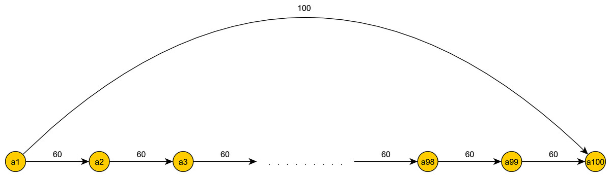
Figure 4: The deadline scheme is preferable.
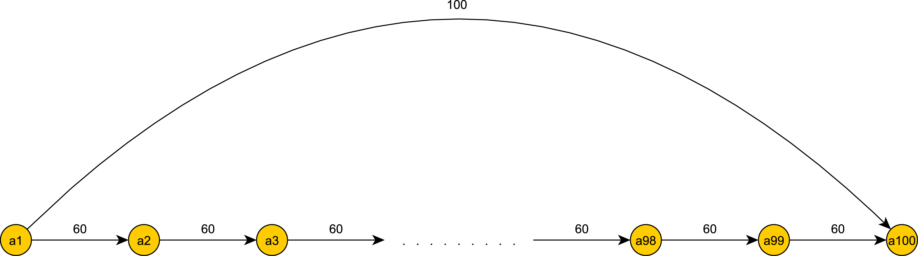
In fact, we used the history scheme in Alg. 1 to detect continuous pattern matches. We can also benefit from using the deadline scheme to detect such patterns, when there are few overpassing edges in the pattern graph.
What is the differential line between using one scheme and not the other? A straightforward calculation follows. Let k be the number of overpassing edges in the graph. Then in the deadline scheme, a token will have O(k⋅log(n) + n) operations. In the history scheme we may have up to O(n2) overpassing edges as in the example in Fig. 4. Thus a starting point for finding the differential line is k = O(n2∕log(n)). Furthermore, depending on the exact configuration of constraints and their values, it may be that in the average case a token’s heap has constant size throughout the graph traversal, as in Fig. 4 where k = 1. In this case, we have a better number of operations and space complexity for the deadline scheme, namely O(n) and O(1), respectively.
Adding minimum constraints
We now broaden our scope by allowing input patterns with both maximum and minimum constraints. We highlight the differences in definitions and notations that ensue. Here a temporal pattern input is a triplet TP = (A, CMax, CMin). A is the sequence of events: A = (a1, a2, …, an). CMax is a set of maximum temporal constraints (max constraints) on A. An element of CMax is (ai, aj, t), where t is the maximum time allowed between ei and ej. CMin is a set of minimum temporal constraints (min constraints) on A. An element of CMin is (ai, aj, t), where t is the minimum time allowed between ei and ej.
We note that a temporal constraint may be 0 or ∞. Furthermore, one may change the model slightly by allowing only strictly positive time intervals for the min constraints, i.e., each constraint is of value at least 1. This simply amounts to adding the constraints (ai, ai+1, 1) to CMin for every 1 < i < n − 1. In general, we may define in our model (or get a restriction as input) that all constraints must be in the time window (m, M) for some where m ≤ M. This amounts to adding the constraints (ai, ai+1, m) to CMin and (ai, ai+1, M) to CMax for every 1 < i < n − 1.
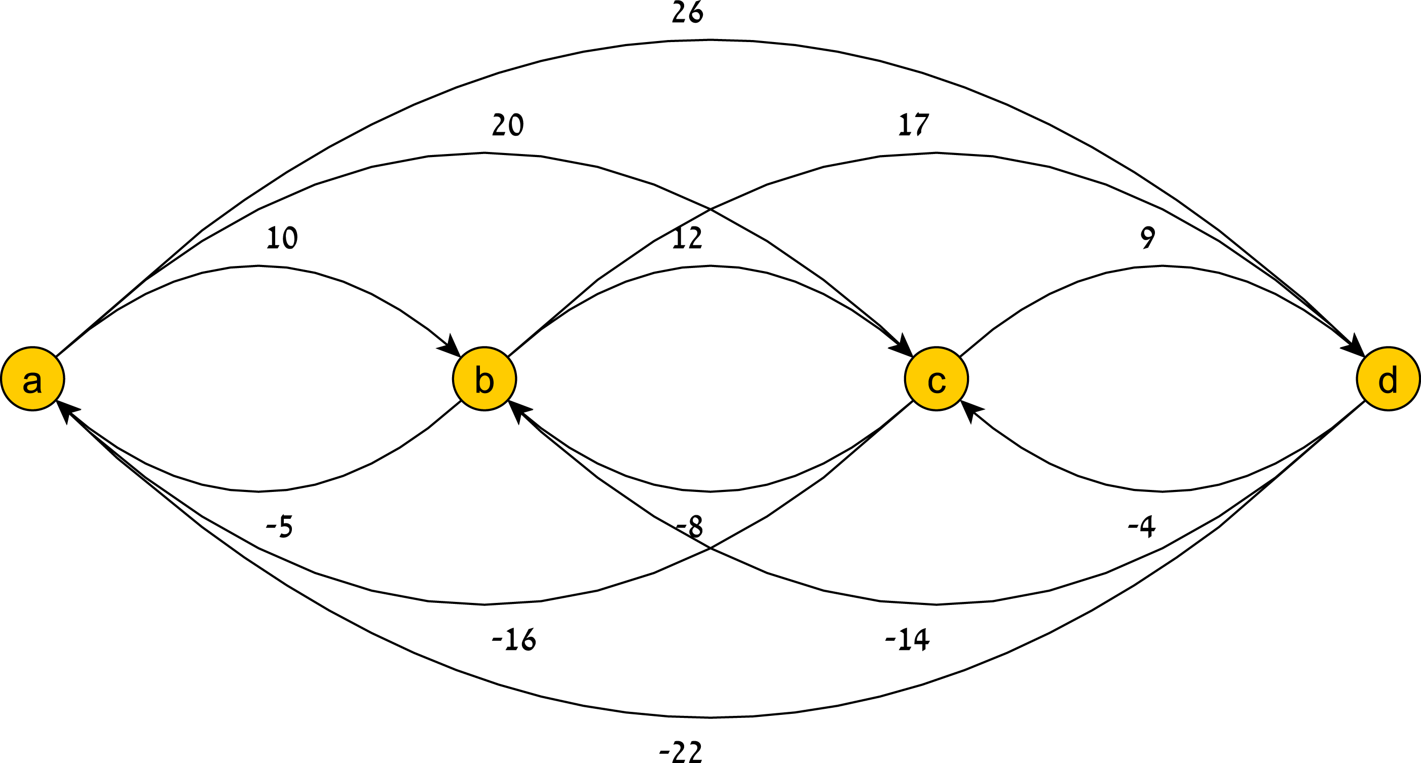
Preprocessing phase. The definition of a history fitting a temporal pattern is similar to ‘Maximum constraints,’ only the history should adhere to both min and max constraints. We describe the preprocessing process. We build a weighted, directed graph G = (A, E), where nodes are the events in A, and edges are E = {(ai, aj, t)∣(ai, aj, t) ∈ CMax}⋃{(aj, ai, − t)∣(ai, aj, t) ∈ CMin}. Also, there’s an edge (ai, ai+1, ∞) or (ai+1, ai, 0) for consecutive events without a constraint in CMax or CMin, respectively. The purpose of this construction is again to utilize the Floyd–Warshall algorithm for finding all shortest paths. Here we will have a “window of opportunity” for every pair of events ai and aj that will indicate the exact time frame in which a token residing on ai must reach aj to hold by the constraints. We call this window a time window for ai and aj. We run the Floyd–Warshall algorithm to find the shortest paths between all pairs of nodes in G. Our purpose is to contract the time windows as much as possible for all pairs of events. An example graph is depicted in Fig. 5.
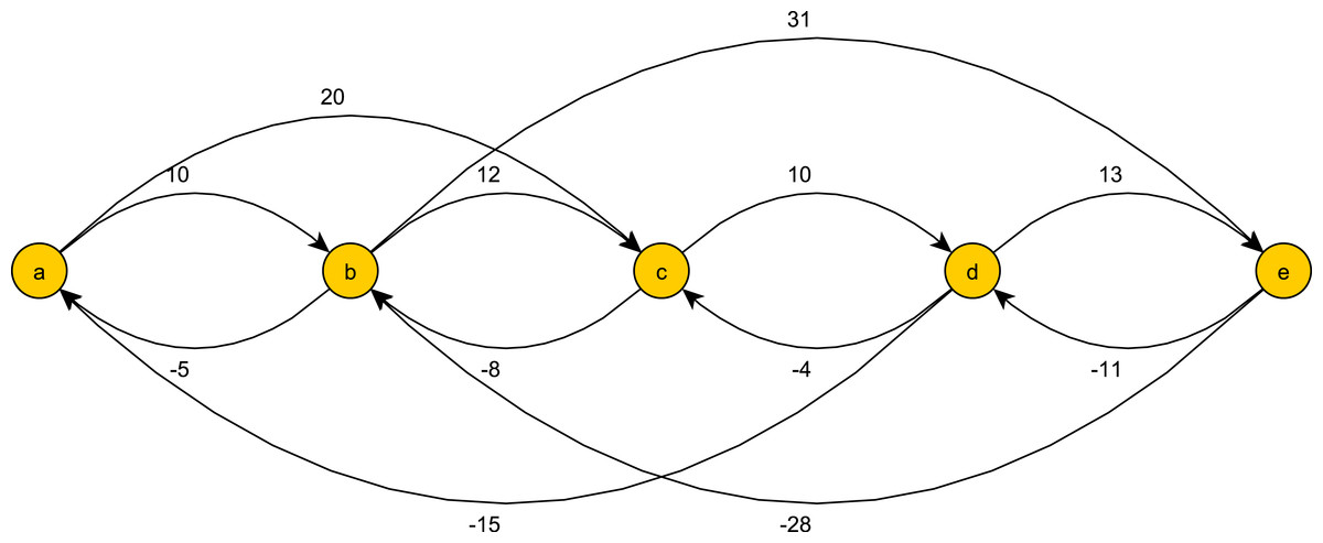
Figure 5: A graph for max and min constraints temporal pattern.
The shortest (b, d)-path, ((b, e)(e, d)), has weight 20. The shortest (d, b)-path, ((d, e)(e, b)), has weight −15. Following the preprocessing phase, we get that tw(b, d) = (15, 20).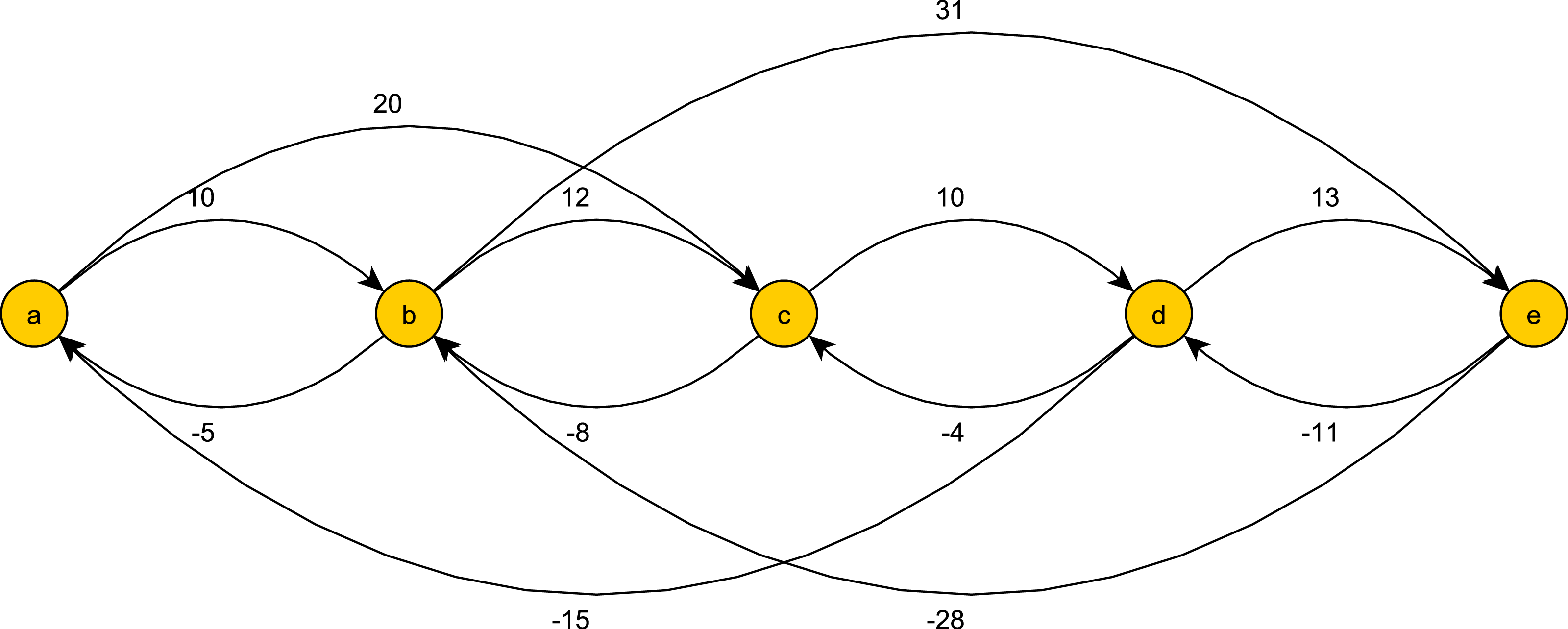
Time windows. Next we define the time windows. Let min(a, b) be the weight of the shortest (a, b)-path. For all 1 < i < j < n: . We denote the set of all time windows of TP as TW(TP). ai and aj are called the source and destination of tw(ai, aj) respectively, and are denoted by src(tw) and dst(tw), respectively. The first index of a time window tw is called the lower bound of tw, denoted as . The second index is called the upper bound, denoted as . A time window between consecutive events ai and ai+1 is called a simple time window. If twi(ai, bi) and twj(aj, bj) are time windows such that (aj ≲ ai∨aj = ai)∧(bi ≲ bj∨bi = bj), we say that twi is subsumed by twj. If H is a history and tw is a time window between events a and b, then H(tw) denotes H(a, b). Formally, we define , , and TP′ = (A, CMax′, CMin′), and show that TP ≡ TP′. TP′ is in fact the temporal constraints closure of TP. These updates maintain temporal constraint semantics (Proposition 2).
Another case to consider is whether the temporal pattern is consistent; whether there is a history that fits the pattern. If, for example, we have the constraints: (a, b, 10), (b, c, 7) ∈ CMax, and (a, c, 24) ∈ CMin, there is a contradiction in the temporal semantics of the temporal pattern, and no history can fit the pattern. However, not all contradictions may manifest in so obvious a fashion. Fortunately, this happens exactly when there is a negative cycle (a cycle with negative weight) in G, something we can detect with a slight modification of the Floyd–Warshall algorithm.
Let TP and TP′ be the temporal patterns before and after the executing preprocessing, respectively. Then the following properties hold:
Equivalence: TP ≡ TP′.
No-Negative: There exists a history H that fits TP⇔ there is no negative cycle in G.
Minimality: Assuming there is no negative cycle in G, then: TP′ is the minimal graph that is equivalent to TP, i.e., any further contraction of any time window in TP′ will result in a temporal pattern TP″ that is not equivalent to TP′.
See Appendix S2 for proof. A different form of the proof has appeared in the framework of Temporal Constraint Networks (Dechter, Meiri & Pearl, 1991), and in particular the no-negative result has appeared in Leiserson & Saxe (1983); Liao & Wong (1983).
On-line detection phase. First, we observe that, unlike Alg. 2 (lines 8–9), an older token from ai+1 cannot be discarded when a new token is spawned, as the older token may complete a pattern match while the new one does not, and vice versa. See Fig. 6 for an illustrating example.
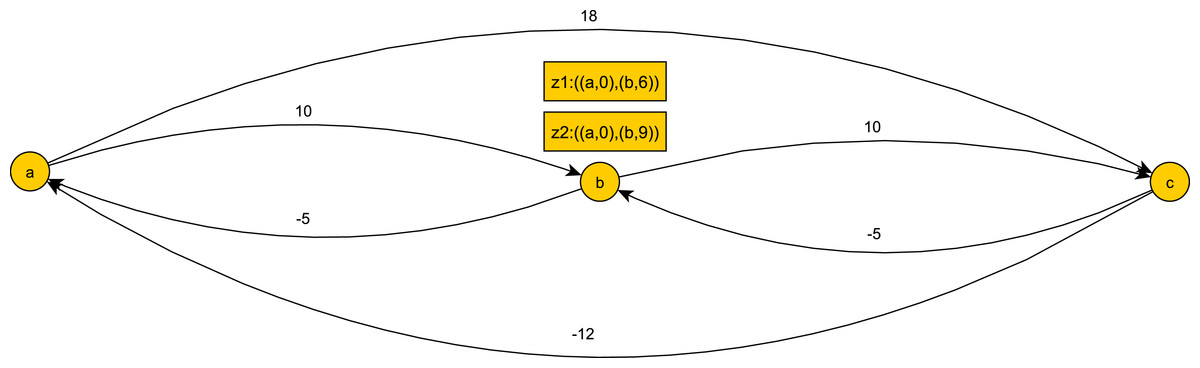
Figure 6: An example of a temporal pattern for min and max constraints after preprocessing.
Given the history ((a, 0), (b, 6), (b, 9)) we have two tokens on b with different histories. If (c, 13) occurs z1 will advance while z2 will not, and if (c, 17) occurs z2 will advance while z1 will not.
Furthermore, we do not have overpassing edges as in ‘Maximum constraints’, but rather time windows. In other words we have overpassing max and min edges between all pairs of non-consecutive events, i.e., Θ(n2) overpassing edges. As shown in Proposition 2, a token on an event ai whose history satisfies the temporal constraints of ai with a1, …ai−1 may complete a pattern match. Hence, if we use the history scheme in keeping a history for each token, whenever the token reaches an event we can check back against constraints with earlier events. Such a simple scheme ensures the earliest detection of an obsolete token. This amounts to keeping an O(n) space history per token, and performing O(n2) total checks per token that traverses the entire graph. Since we have Θ(n2) overpassing edges, it seems at a first glance that the deadline scheme is not efficient, since we have n2⋅log(n) operations and O(n) space per token, as in ‘Maximum constraints.’
However, if we examine the temporal pattern depicted in Fig. 4 where all min constraints are 0, we see that we need to save only one deadline for a token and perform O(n) checks in total, which is better than the history scheme. Defining all time windows is unnecessary and is in fact a hindrance, since the time windows do not add information; the given graph already follows the temporal constraints closure of the temporal pattern. Using the history scheme here is inefficient: Roughly speaking, as the graph gets richer with more max and min constraints, the history scheme becomes more plausible, since the preprocessing phase will yield much more information in the form of contracted time windows.
Prediction and Alert of a Near Pattern Match
We conduct an analysis to estimate the chances of a token representing a partial pattern to complete a pattern match, henceforth the token’s completion probability. We assume events of all types have equal probability p of occurring at any time point.
Probabilistic settings. Our computation advances in parallel to the chronological order of the pattern events. For each event we reach, we examine the distinct possibilities of the next event (or rather, its type) occurring in the desired time frame—in the necessary time window. We start with a basic example to illustrate the computation process.
Assume we have a two event temporal pattern with events a0, a1 and a time window tw(a0, a1) = (m, M). Let a0 occur at time 0, so that we have a token on a0 representing a partial pattern P0. We have M − m + 1 distinct possibilities for P0 to complete. The probability of a1.type not occurring at times m, m + 1, …, m + j − 1 and occurring at time m + j for some 0 ≤ j ≤ M − m, is (1 − p)jp. We define pj = (1 − p)jp. We shall also refer to elements of the form pj as probability factors.
Now, assume we have a temporal pattern TP with n + 1 events, a0, …, an. We start with a simple example where the pattern graph has only simple edges (for both max and min constraints). In such a case, if the probability of a token advancing from a0 to a1 is p(1) and the probability of it later advancing from a1 to a2 is p(2), then the probability of the token getting from a0 to a2 is p(1)⋅p(2). The overlying fact that governs this result is the lack of dependencies between the two advancement steps, which is in turn due to the lack of an overpassing edge that encompasses the interval of events from a0 to a2. To generalize, if the probability of a token advancing from ai−1 to ai is p(i), then we get in this case that the completion probability of a token at the beginning of the temporal pattern is . If tw(ai−1, ai) = (mi, Mi), 0 ≤ i ≤ n − 1, then we get that the precise completion probability is .
Now, assume we have some general pattern where there may be overpassing edges in the pattern graph. Say we have a token residing on ai, with a partially fitting history : H may (and probably does) limit the times at which the token may reach subsequent events. In other words, it further contracts the time windows of TP for this token. Next, we examine how a token’s history impacts the subsequent time windows and the computation of the token’s completion probability.
History restrictions and induced pattern graphs
First we provide some notational groundwork. Let TP = (A, CMax, CMin) and let . We define TP|H = (A, CMax∪C(H), CMin∪C(H)). In other words, C(H) is the set of constraints defined by the history H, and TP|H is the restriction of TP to temporal patterns that admit only histories that contain H as their fitting histories. We define G(TP) as the graph (A, E), where the nodes in A are the events of TP, and the edges are . In other words, G(TP) is the pattern graph induced by TP∗ (the closure of TP, see ‘Adding minimum constraints’). For a pattern graph G = (A, E) and a partially fitting history H, we define EMax = {(ai, ai+1, H(ai, ai+1)}1≤i≤|H|−1, EMin = {(ai+1, ai, − H(ai, ai+1)}1≤i≤|H|−1, and G|H = (A, E∪EMax∪EMin).
Illustrations of a temporal pattern graph and its restriction to a history are shown in Figs. 7 and 8, respectively.
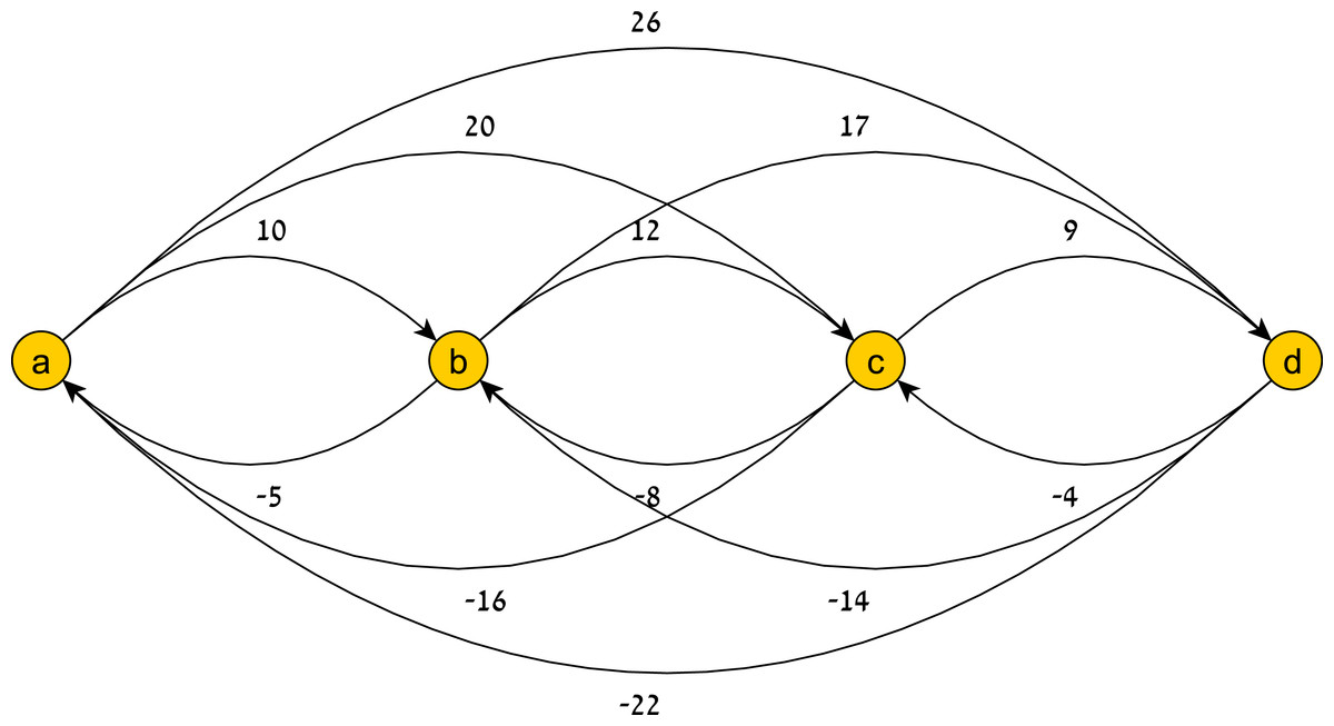
Figure 7: A temporal pattern graph G(TP).
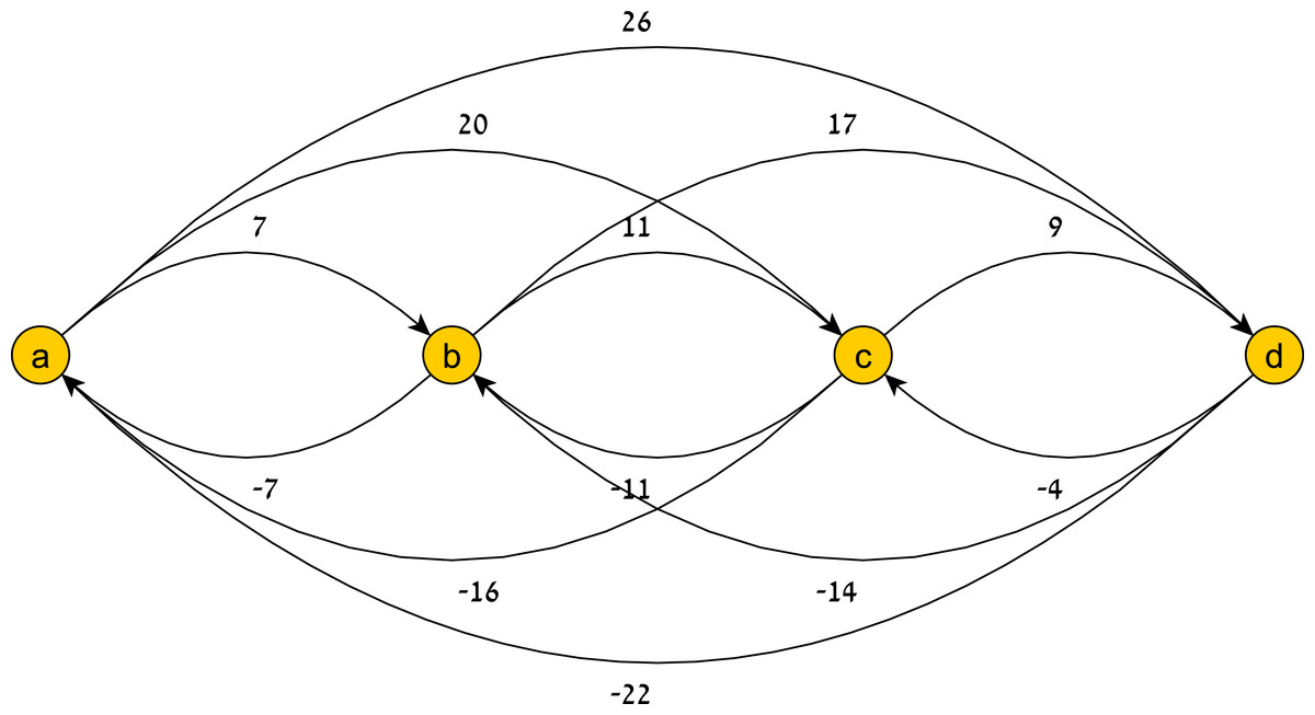
Figure 8: A history-restricted pattern graph.
The graph G(TP|H) of TP’s restriction to the history H = ((a, 0), (b, 7), (c, 18)).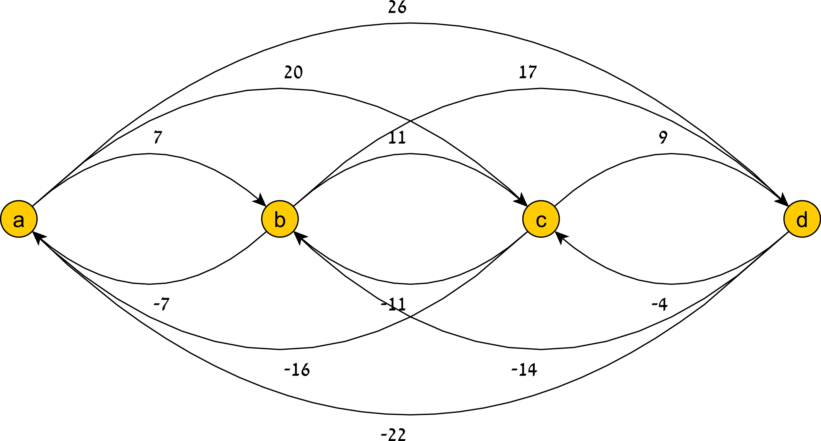
Note that the new edges defined by H replace the old ones (they are more restrictive). Simply put, the induced graph represents a new temporal pattern that includes H in its account of temporal constraints. If the time that passed between events ai and ai+1 in H is t, and if we wish to define a new temporal pattern that admits only histories containing H as a subset, we should add the (both max and min) temporal constraint (ai, ai+1, t).
In order to compute the time window defined by H between events ar and ar+1, we need to find the shortest (ar, ar+1)-path and (ar+1, ar)-path in G|H. If the probability of this distinct history is p(H) = pj1pj2…pji, and the time window defined by H for reaching ai+1 is of size k′, then we have k′ + 1 branchings of possible continuations of H and appropriate probability factors added to p(H). Namely, the branchings and their probabilities are pj1pj2…pjipjl , 0 ≤ j ≤ k′. If , we denote as . If l is clear from the context, we simply write .
Thus, if we have a token residing on the first event of a temporal pattern and we wish to compute its completion probability, we should sum up all the possible history branches and their probabilities. We can envision this branching computational process as a tree of histories, where each (full and fitting) history will be a path from the root of the tree to a leaf, representing a distinct probability of a token completing to a pattern match. We therefore sum all the possibilities (defined by distinct histories) of a token completing to a pattern match, and add-up to get the desired completion probability of the token.
We recall the definition of a temporal pattern’s girth: . Thus, for a temporal pattern TP with n events, and g(TP) = k, the calculation of the completion probability for a token on the first event will take O(d⋅kn) time, where d is the time it takes to compute the shortest (ai, ai+1)-path and (ai+1, ai)-path for every 1 ≤ i ≤ n − 1.
A more tractable problem is predicting the completion probability of a token residing on an event ai, where n − i is bounded by some small l. We then get an O(d⋅kl) time complexity for calculating a token’s completion probability. Hence, for a small enough l, say l = O(logkn), we get a time complexity of O(d⋅n). To generalize, if l = O(polylogk(n)), we get a time complexity of O(d⋅poly(n)).
Recomputing the shortest paths between consecutive events
Finding the size of the next time window at each level of the probability tree can be done in linear time due to the following fact: The shortest (ar, ar+1)-path and (ar+1, ar)-path in G(TP|H) for some 1 ≤ r ≤ n − 1 and a partially fitting history must take the form of using a series of edges out of the new simple edges induced by H and a single overpassing edge from the beginning of this series to ar+1. Fig. 9 is an illustration of these paths.
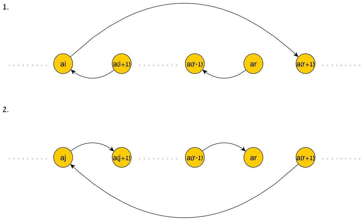
Figure 9: An illustration of the shortest paths induced by a history.
An illustration of the shortest paths induced by H. 1. illustrates the shortest (ar, ar+1)-path and 2. illustrates the shortest (ar+1, ar)-path.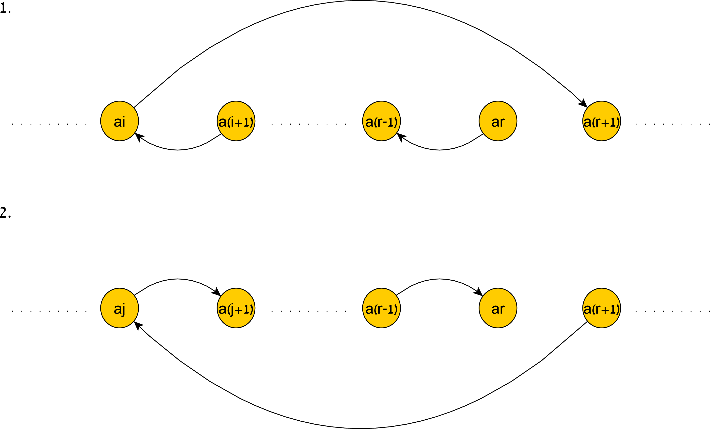
The following lemma formalizes this fact.
Let TP be a temporal pattern, and let for some 1 ≤ r ≤ n − 1 be some partially fitting history of TP. Then the following hold:
∙The shortest (ar, ar+1)- path in G(TP|H) is ((ar, ar−1, H(ar−1, ar)), (ar−1, ar−2, H(ar−2, ar−1)), …, (aj+1, aj, H(aj, aj+1)), (aj, ar+1, w))for some 1 ≤ j ≤r, where (aj, ar+1, w) is a maximum constraint in TP∗.
∙The shortest (ar+1, ar)- path in G(TP|H) is ((ar+1, aj, w), (aj, aj+1, H(aj, aj+1)), (aj+1, aj+2, H(aj+1, aj+2)), …, (ar−1, ar, H(ar−1, ar)))for some 1 ≤ j ≤r, where (ar+1, aj, − w) is a minimum constraint in TP∗.
See Appendix S2 for proof.
As a result of Lemma 3, we get that computing the completion probability of a token residing on an event ai in a temporal pattern TP, where n − i is bounded by some small l takes O(n⋅kl) time complexity, where k = g(TP). If l = O(logkn) we get an O(n2) time complexity. Generally, if l = O(polylogk(n)), we get a time complexity of O(poly(n)).
Also note that if l and k are bounded, we get a time complexity that is linear in n.
Aggregating completion probabilities
We summarize how the completion probability can be computed using a polynomial-size data structure to reduce the number of arithmetic computations. Due to space considerations, the complete algorithm is not shown.
We recall our discussion of the tree of histories which we call a probability tree. Each history is a path from the root down to a leaf. The root represents the token’s relative zero-time, i.e., the time from which we wish to compute the token’s completion probability. An edge Pxi to a node in the tree represents a time point with a shift of xi time points relative to the beginning of the current time window, contributing a factor of pxi to the current probability path. The set of a node’s children in the tree represents the different possibilities of the current history’s continuation. In other words, suppose the current probability path counts the factors . If we compute , we have . Suppose the next time window is of size k′, then the edges to the current node’s children are P0, P1, …, Pk′, and continuing along an edge Pxd+1, 0 ≤ xd+1 ≤ k′ adds the factor pxd+1 to the above multiple, yielding .
What we get here is in fact multiple paths that lead to the same probability. Let T be a probability tree, and let Paths(T) be the set of rooted paths in T ending in a leaf. Then the token’s completion probability equals , where ρ(P) denotes the value of the last node in P.
Furthermore, if TP is the temporal pattern and k = g(TP), then the maximal value of a leaf is k⋅l, since every node along a path from the root to the leaf contributes at most a factor of . Hence, there are at most k⋅l + 1 leaves and we can use an array of size k⋅l + 1 to count the instances of every , 0 ≤ j ≤ k⋅l.
Concluding Remarks
In this work we introduced a novel framework for monitoring real-time systems for undesired behavior, based upon specifications given as temporal patterns. The system specifications are described using temporal constraint semantics. Instead of modeling and searching the system for its entire state-transition graph, as done in model checking, we proposed an approach to verify sequence of system events at runtime with time restrictions over the events. We devised a process for finding the closure of the temporal constraints semantics to reduce the pattern constraint set while maintaining the temporal constraint semantics, and provided different schemes for on-line detection of temporal patterns. The earliest possible notification on completed patterns helps the system to reduce number of comparisons during systems’ pattern match execution. An analysis is provided to predict and estimate the chances of a token representing a partial pattern to complete a pattern match.
A summary of complexity measures for handling different pattern types and schemes is shown in Table S1.
Specifications of properties for on-line verification may be more complex. Hence, another line of research may broaden the input scope of temporal patterns as boolean formulae, where constraints are variables and histories are assignments. We say H fits a temporal pattern formula if it evaluates to True under H. We define the language TP-SAT as all temporal pattern formulae TP, such that there exists a history H that fits TP. TP-SAT ∈ NP, and it is easy to show by a reduction from SAT that TP-SAT is NP-Hard. However, some families of formulae may be tractable. The DNF formulae, for example, may be seen as a collection of regular temporal patterns with the same sequence of events (albeit different temporal constraints), and handled accordingly.
Furthermore, the probabilistic settings may be expanded to include different probabilities for different event types, though the computations would be similar. Setting non-uniform distributions on the other hand may necessitate a different approach.