
Continuous authentication using deep neural networks ensemble on keystroke dynamics
- Published
- Accepted
- Received
- Academic Editor
- Mamoun Alazab
- Subject Areas
- Human–Computer Interaction, Artificial Intelligence, Data Mining and Machine Learning, Security and Privacy
- Keywords
- Keystroke analysis, Biometric user identification, Ensemble learning, Deep learning, Neural networks
- Copyright
- © 2021 Aversano et al.
- Licence
- This is an open access article distributed under the terms of the Creative Commons Attribution License, which permits unrestricted use, distribution, reproduction and adaptation in any medium and for any purpose provided that it is properly attributed. For attribution, the original author(s), title, publication source (PeerJ Computer Science) and either DOI or URL of the article must be cited.
- Cite this article
- 2021. Continuous authentication using deep neural networks ensemble on keystroke dynamics. PeerJ Computer Science 7:e525 https://doi.org/10.7717/peerj-cs.525
Abstract
During the last years, several studies have been proposed about user identification by means of keystroke analysis. Keystroke dynamics has a lower cost when compared to other biometric-based methods since such a system does not require any additional specific sensor, apart from a traditional keyboard, and it allows the continuous identification of the users in the background as well. The research proposed in this paper concerns (i) the creation of a large integrated dataset of users typing on a traditional keyboard obtained through the integration of three real-world datasets coming from existing studies and (ii) the definition of an ensemble learning approach, made up of basic deep neural network classifiers, with the objective of distinguishing the different users of the considered dataset by exploiting a proper group of features able to capture their typing style. After an optimization phase, in order to find the best possible base classifier, we evaluated the ensemble super-classifier comparing different voting techniques, namely majority and Bayesian, as well as training allocation strategies, i.e., random and K-means. The approach we propose has been assessed using the created very large integrated dataset and the obtained results are very promising, achieving an accuracy of up to 0.997 under certain evaluation conditions.
Introduction
The problem of user authentication has been addressed in numerous research studies. Various algorithms faced it exploiting the analysis of keystroke dynamics (Pin Shen Teh & Yue, 2013; Revett, de Magalhães & Santos, 2007) and also recent studies assume that the comprehension of the typing patterns of people can be useful to distinguish or authenticate individuals (Maheshwary & Pudi, 2017; Dhakal et al., 2018; Venugopal & Viji, 2019). Many of these approaches employ techniques relying on either simple statistical machine learning (Maxion & Killourhy, 2010; Ahmadi et al., 2020) or neural network algorithms (Darabseh & Siami Namin, 2015); moreover, they successfully mine some typing patterns such as the timing of a single keystroke (Maheshwary & Pudi, 2017a), the pressure applied when typing (Dhakal et al., 2018), or, referring to mobile and smartphone keystroke dynamics, some other mobile device-specific features (i.e., the device positioning, the accelerometer data, the dimension of the key touch area and the position of the touch) (Revett, de Magalhães & Santos, 2007; Hellström, 2018).
Therefore, keystroke analysis has already proven to provide a significant contribution in improving existing computer security systems, e.g., by means of a new security layer allowing one to ensure a more efficient individual identification as well as to solve some vulnerabilities of traditional authentication approaches (Dowland, Furnell & Papadaki, 2002; Bergadano, Gunetti & Picardi, 2002). As a matter of fact, traditional password-based authentication approaches (Patel et al., 2020) can be easily compromised and they are mainly based on a single authentication judgment whenever a session starts (Dowland, Furnell & Papadaki, 2002). Within such a context, keystroke analysis can be effectively exploited together with the existing authentication systems to ensure a more robust identification, to be performed continuously during every user session. This could be used to avoid, for example, the authentication on the part of a legitimate user and the subsequent usage of the computer, or smart device, by other people while the genuine user is away for a short time. Moreover, a keystroke-based authentication could prove extremely useful in contexts wherein a large number of users can access legitimately a single shared device as well as in common Cloud services.
Furthermore, keystroke analysis approaches applied to user authentication are not intrusive. Indeed, the flow of events produced by recording the stream of typed keys can be analyzed in real-time with different techniques and without any interference with the behavior or activity of the user. Finally, while existing key-loggers can easily support keystroke analysis, they are also useful to collect different events taking place in the user typing, thus allowing the storage of more significant data with low costs.
Based on the aforementioned considerations, several machine learning algorithms have been proposed to conduct keystroke analysis in the past years (Revett, de Magalhães & Santos, 2007; Muliono, Ham & Darmawan, 2018). Nevertheless, several limitations need to be overcome. Indeed, these algorithms are mainly based on a limited group of features or assessed on limited datasets. As a consequence, the use of deep learning approaches to perform keystroke-based authentication is very limited, as it requires large and balanced datasets to successfully train the deep neural network model itself.
Nevertheless, the advantage of using a deep learning approach in keystroke analysis is clear and it is highlighted in several contributions, such as the one in Sundararajan & Woodard (2018), wherein the authors assert that deep learning techniques could be suitable to perform biometric recognition, or the one in Çeker & Upadhyaya (2017b), where deep learning techniques are demonstrated to be able to strengthen the capacity of all the considered features and to manage large intra-class changes and noisy biometric data.
In order to overcome these gaps, this paper proposes a multiple classifier approach, based on basic deep neural networks gathered into a unique ensemble classifier, in order to perform keystroke analysis activities by means of a generalizable feature model. The evaluation of the proposed approach, which is an expansion of the preliminary study described in Bernardi et al. (2019), was performed by using the integration of three pre-existing well-known datasets.
In summary, the main contributions this study can offer on the matter are the following:
-
the design and description of a large group of unique features characterizing the properties of the typing events of a user;
-
the modeling of a process for the integration of different keystroke datasets, based on the defined feature model, into a large integrated dataset composed of 169,678 different users;
-
the design of an ensemble deep learning approach, for mining and successfully exploiting the very large keystroke dataset we built, which exploits different allocation and voting strategies;
-
the performing of several experiments and evaluations, using the very large integrated dataset, useful to assess the validity of both the designed feature model and the ensemble deep learning classifier.
The rest of this paper is structured as follows: the second section discusses the related work and the background. The third section presents the feature model we adopted and the classification approach we propose. The fourth section provides the evaluation and the discussion of the obtained results, while the fifth section contains some considerations about the validity of the used approach. Finally, the last section draws some conclusions and future research directions.
Related Work and Background
Keystroke dynamics analysis
During the past years, the problem of user identification has been tackled through various algorithms based on the analysis of keystroke dynamics (Pin Shen Teh & Yue, 2013; Venugopal & Viji, 2019). Many of these approaches employ techniques relying on either simple statistical machine learning (Maxion & Killourhy, 2010; Ahmadi et al., 2020) or neural network algorithms (Darabseh & Siami Namin, 2015). Statistical machine learning approaches carry out keystroke classification by using some of the following techniques: K-Nearest Neighbours (KNN), Naive Bayes classifier (NB), Support Vector Machines (SVM), etc.; among these, SVM algorithms provide the most promising results. A statistical approach is used in Roh, Lee & Kim (2016), wherein the authors implement classifiers with five features measured by means of smartphone sensors. In Alpar (2019) a frequency-based authentication system called TAPSTROKE is proposed. The experiments are conducted by using a one-class SVM with a simple linear kernel for both Hamming and Blackman window functions. A random forest (RF) classifier is proposed in Alshanketi, Traore & Ahmed (2016) to improve accuracy performance in the mobile keystroke dynamic biometric authentication. The evaluation is performed on two public datasets and an ad-hoc built dataset. The authors in Kang & Cho (2015) also study typing patterns of users digitizing long and free text strings from various input devices, by evaluating different statistical methods. Finally, in Wesoowski, Porwik & Doroz (2016), four classifiers (C4.5, BN, SVM, and RF) in an ensemble approach are used to support electronic health record security. A more recent approach (Lu et al., 2020) proposes a deep neural network model (convolutional neural networks + recurrent neural networks) to learn the keystroke data of free texts. The approach is validated on an existing dataset giving interesting results. Considering always the neural networks approach, several studies (Kim, Lee & Shin, 2020) are also focused on the definition of feature-selection methods. In Loy, Lai & Lim (2007), for example, the authors performed user classification by using perceptrons, back-propagation, and ART-2 network. However, such approaches require a long time to train the model and are mainly based on some manual tasks. Moreover, these models are also difficult to be generalized (Deng, Heaton & Meltzner, 2014).
More recently, keystroke dynamics techniques have been used to authenticate a computer user in the background, while the user is actively working at a terminal (Ceker & Upadhyaya, 2017a). In particular, the authors investigated the applicability of deep learning on three different datasets by using convolutional neural networks and Gaussian data augmentation techniques. In Chu-Hsing Lin (2018) recorded scan codes and keystroke sequences of passwords are used to distinguish the legitimate users from the non-legitimate ones by using deep convolutional neural networks (CNNs). When comparing the detection rates between the CNN and a traditional neural network, the authors proved that the CNN is the best choice. In Alpar (2017), the biometric keystroke authentication is performed using Gauss-Newton-based neural networks to classify frequency spectrograms. The goal of this study is to perform frequency authentication to enhance keystroke authentication protocols.
Table 1 reports a summary of the characteristics of the above-described approaches. The table highlights for each study the kind of classification approach, the adopted data type (free text and fixed text), the number of users involved in the experimentation, and the reached Equal Error Rate (EER).
| Approach | Reference (Year) | Data type | #Users | EER |
|---|---|---|---|---|
| Trigram-based Single DNN 7 layers (10 users) | This work | Free Text | 1000 | 1.11% |
| Trigram-based Single DNN 7 layers (100 users) | 2.87% | |||
| Trigram-based Ensemble DNN 7 layers (10 users/cluster) | 1.58% | |||
| Trigram-based Ensemble DNN 7 layers (100 users/cluster) | 2.95% | |||
| Ensemble classifiers | Porwik, Doroz & Wesolowski (2021) | Free Text | 150a | 0.15% |
| Convolutional neural network + Recursive neural network | Lu et al. (2020) | Free Text | 260 | 2.67% |
| Modified STFT + Hamming | Alpar (2019) | Fixed Text | 24 | 1.76% |
| Modified STFT + Blackman | 2.60% | |||
| STFT + Hamming | 8.50% | |||
| STFT + Blackman | 9.72% | |||
| Convolutional neural networks (CNN) | Ceker & Upadhyaya (2017) | Free Text | 39 | 2.16% |
| GN-ANN | Alpar (2017) | Fixed Text | 12 | 4.10% |
| Random Forest (Pressure + finger area) | Alshanketi, Traore & Ahmed (2016) | Fixed Text | 103 | 5.65% |
| Random Forest (DT + FT + Pressure + finger size) | 2.30% | |||
| Statistical | Roh, Lee & Kim (2016) | Fixed Text | 15 | 7.35% |
| Statistical | Kang & Cho (2015) | Free Text | 35 | 5.64% |
| Ensemble (C4.5, Bayesian Network, SVM, Random Forest) | Wesołowski, Porwik & Doroz (2016) | Free Text | 29a | 2.17% |
| Random Forest | Maxion & Killourhy (2010) | Fixed Text | 28a | 8.6% |
| ARTMAP-FD | Loy, Lai & Lim (2007) | Fixed Text | 100 | 11.78% |
Notes:
The table shows that all the approaches give a good performance, but they are mainly evaluated on a limited number of users and reach interesting performance only for a small number of them. However, a very large benchmark dataset to be used in comparing quantitatively deep learning techniques with existing machine learning approaches, in the field of keystroke biometric analysis, is not yet published. This is mainly due to the common unwillingness to freely publishing large datasets with suitable features.
Starting from the aforementioned observations, concerning user identification, in this paper, we analyze the performance of a hierarchical multiple Deep Neural Network (DNN) classifier learning algorithm that uses an accurately designed set of features. To obtain a larger and varied dataset, we combined three existing datasets. This allowed us to validate our approach using data from different typing scenarios, a scenario rarely tackled in the literature.
Deep learning algorithms
Deep Learning (DL) algorithms have been used in the last years in several domains becoming more and more diffused ( Zhao et al., 2020; Yang et al., 2020; Junseob Kim, 2020). They expand classical machine learning techniques by adding more complexity into the model and transforming the data using various functions which hierarchically represent them. This is usually done through several levels of abstraction, in turn, composed of various artificial perceptrons (Yu & Deng, 2011). Indeed, DL neural networks simulate the way biological nervous systems process information. In particular, these approaches are based on neural networks made up of several hidden layers, whose input data are transformed across several steps with different abstract and composite representations, which realize pattern classification and feature learning through a hierarchy of concepts.
The training of a DL network resembles that of a simple artificial neural network and consists of the following phases: (i) a forward phase, in which the activation signals of the nodes, usually triggered by non-linear functions, are propagated from one layer to the following one, and (ii) a backward phase, allowing the modification of the weights and biases, if necessary, to enhance the network performance.
DL is suitable to solve complex problems particularly well and quickly, by employing black-box models that can increase the overall performance (i.e., increase the accuracy or reduce the error rate). Because of this, DL is getting more and more widespread in several complex domains of different nature (Alom et al., 2019; Yang, Venkatraman & Alazab, 2018; Alazab et al., 2020; Vasan et al., 2020; Zhaoet al., 2020).
Ensemble learning
Ensemble learning (Dietterich, 2000) consists in grouping a set of classifiers together in order to classify new instances in a combined fashion, i.e., the decision of each classifier is taken into account as a vote and all votes are combined, according to specific rules, producing a final overall classification decision as its output.
Ensemble learning methods, which create a sort of super classifier, are in general much more accurate than any single composing classifier by itself (Hakak et al., 2021). This is because algorithms that output a single hypothesis suffer from three issues (partly solved by ensembling techniques): (i) the statistical problem, (ii) the computational problem, and (iii) the representation problem. These issues are usually solved by minimizing the following two kinds of errors: variance in sensitivity and bias in the model itself.
Ensemble learning usually employs the same basic classifier repeated n times and the output of each classifier is different because different samplings of the training data are used or random parameters are present in the single basic classifier itself.
As a matter of fact, ensemble methods can be classified according to the following: (i) their training allocation strategy and (ii) the type of combination of the outputs (votes) (Bishop, 2006).
Concerning the training allocation strategy, bagging provides parallel training with different training sets (through random allocation or clustering according to specific rules), boosting employs sequential training by re-weighting the samples, while the mixture of experts encompasses parallel training with labor division.
Concerning the combination of the outputs, different choices could be made, such as the following:
-
unweighted average (Ju, Bibaut & van der Laan, 2018), which provides the mean of the output votes for all basic classifiers, is the most common approach in the case of similar component classifiers of comparable performance. In the case of classification problems, the amount to be averaged corresponds to the predicted probability after a softmax transformation, computed according to the following formula: (1) where si is a score vector, output of the last layer of the neural network for the ith unit, si[k] is the score corresponding to the kth class, and pij is the predicted probability for unit i in class j.
-
majority voting (Kokkinos & Margaritis, 2014), which counts the votes per label of all basic classifiers and decides using the label with most votes. It is less sensitive to the output coming from a single basic classifier than the unweighted averaging strategy.
-
Bayesian voting, which states that each basic classifier outputs a hypothesis hj(x, y), where x is the array of features and y the class associated to a sample to be tested. The Bayesian optimal classifier determines the class y according to the following criterion: (2) where P(hj) is the prior distribution of hj, usually considered uniform, Strain the training set of classifier j, and P(Strain|hj) the likelihood of the data under the hj hypothesis.
-
stacking, which linearly combines all predicted outputs from the basic classifiers, wherein each output is opportunely weighed through a weight vector learned by means of a proper meta-learner. For example, predictions f1, f2, …, fm can be linearly combined with weights ai, i ∈ 1, …, m according to the following equation: (3)
In this paper, we investigate the performance of the proposed ensemble classifier, described in the following, by adopting both majority and Bayesian voting approaches.
Approach
In this section, we describe carefully the approach used to identify users by means of their typing dynamics. The approach is based on three essential components:
-
the feature model;
-
the ensemble or hierarchical multiple classifier;
-
the basic classifiers of the ensemble, exploiting deep neural networks.
In the following subsections, these three components are thoroughly detailed and explained.
Features model
The approach we propose is based on the assumption that users can be identified by analyzing their typing dynamics. In this subsection, we describe a set of features allowing the capture and discrimination of such typing dynamics. Each proposed feature permits the representation of a specific aspect of user typing dynamics and is obtained from our previous analysis and from the study of the relevant literature (Killourhy & Maxion, 2009; Banerjee et al., 2014; Feit, Weir & Oulasvirta, 2016).
The proposed model stems from the definition of the concept of keystroke stream. Considering the release of a key as a key up (U) event and the pressing of a key as a key down (D) event, respectively, we can define a keystroke stream as a set of typing events as follows: (4) where: (5)
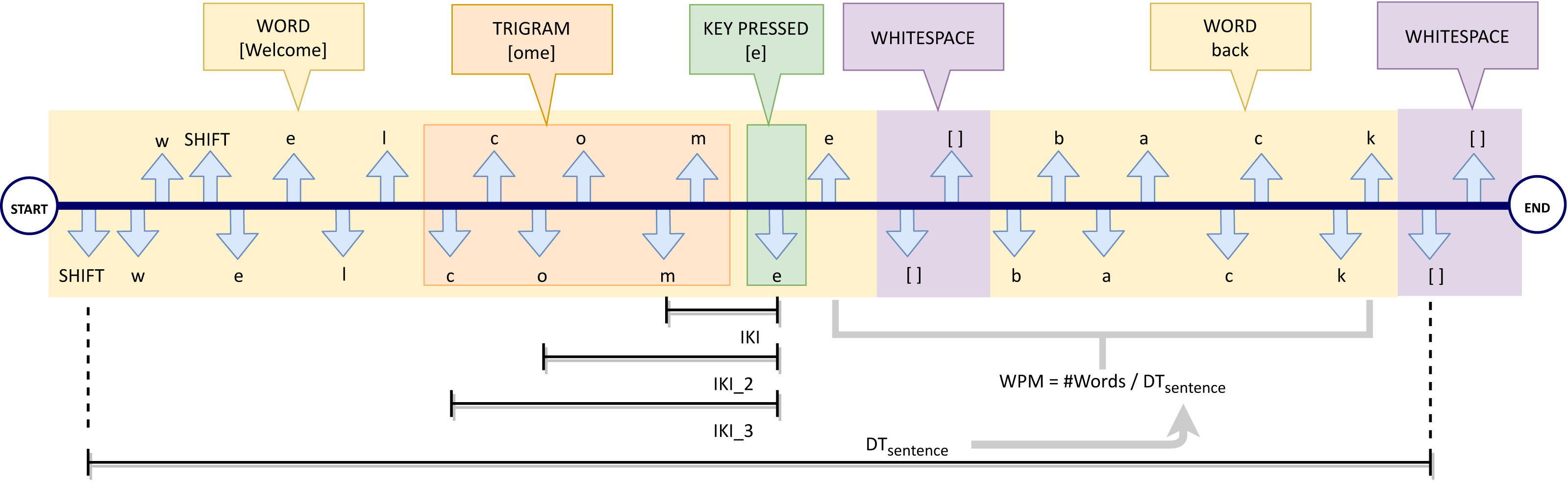
Hence, a typing event Ei is represented as a triple composed of a key code ci belonging to the set N of all possible codes, an event type (D means ‘press’ and U means ‘release’) and a timestamp ti (the temporal instant when the event took place). Figure 1 shows an example of a keystroke stream, obtained when a user writes the sentence “Welcome back”. Each typing event is represented by means of down arrows for the pressing of a key and up arrows for the release of a key.
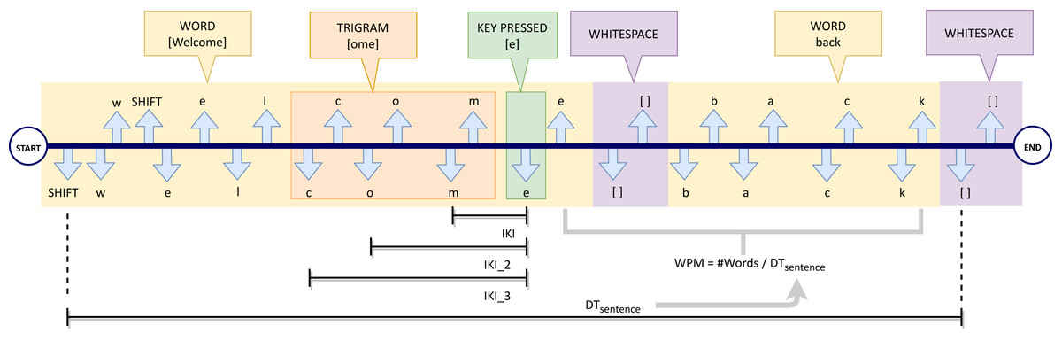
Figure 1: Example of a keystroke stream.
Looking at the stream described in the example above, in a flow of f typing events a sentence S can be seen as a sequence of m words (with m ≤ f): (6) Moreover, Fig. 1 shows how each word Wi is delimited by word-breaking (https://unicode.org/reports/tr29/#Word_Boundaries) characters according to the Unicode standard (The Unicode Consortium, 2011) (e.g., the two highlighted white-space divide the keystroke sequence into two words W1 =“Welcome” and W2 =“back”).
For each typing event Ei = (ci, D, ti) (e.g., the ci =’e’ key-down event highlighted in green in the example), we also consider the three previous typing events ([Ei−3, Ei−2, Ei−1]) associated with the previous trigram (e.g., the character stream {(c,D, ti−3), (o, D, ti−2), (m, D, ti−1)} of the figure).
Starting from the aforementioned notations, we computed the following features:
-
Inter Keys Interval (IKI): It is the time (in milliseconds) intervening between two subsequent key-down events. If IKIi is the inter keys interval of a generic typing event Ei = (ci, D, ti), it can be calculated, based on the previous press event, as follows: (7) where ti and ti−1 are the timestamps of the press events Ei and Ei−1, respectively. Referring to Fig. 1 as an example, IKIi is the time interval between the key-press event of the ‘m’ character and the consecutive character ‘e’ (ith event, highlighted in green).
-
Inter Keys Interval (IKI_2): It measures the time interval (in milliseconds) between the last key-down event and the central key down of the previous trigram. If IKI_2i is the IKI_2 of a generic typing event Ei = (ci, D, ti) , it can be calculated as follows: (8) where ti−2 is the instant when press event Ei−2 took place. Referring always to Fig. 1, IKI_2i is the time between the key-press event ‘o’ and the event ‘e’ (ith event, highlighted in green).
-
Inter Keys Interval (IKI_3): It measures the time interval (in milliseconds) between the last key down event and the first key down event of the last trigram. If IKI_3i is the IKI_3 of a generic typing event Ei = (ci, D, ti), it can be computed in the following way: (9) where ti−3 is the time of key press event Ei−3. Referring to Fig. 1, IKI_3i is the time interval since the key-press of ‘c’ and the key-press of ‘e’ (ith event, highlighted in green).
-
Words per minute (WPM): It is the words per minute rate, computed by sentence. For example, considering sentence S made up of m words, its WPM is equal to m divided by the difference between the timestamp of the last key-up event of the final word Wm (tewm) and the timestamp of the first key-down event of the starting word (tsw1). Therefore, its computation is performed as follows: (10) Figure 1 shows an example of WPM calculation for the sentence “Welcome back”. DTsentence is indicated in the figure as the time required to write the whole sentence, made up of m = 2 words.
-
Error Corrections (EC): it is the frequency of “Delete” (DEL) or “Backspace” key-press events during the typing (i.e., the number of removed characters per minute). Even if error correction operations are not limited to these events (for example, users can exploit the pointer or other keys to mark and remove the text), here, we focus only on the events that can be easily extracted from logs of existing applications. Indeed, even if the EC metric does not take into account all possible kinds of text manipulations, it is considered very representative of the mistake frequency of the user and hence highly distinctive.
Finally, the model is completed by adding some aggregated metrics, i.e., average (AVG), variance (VAR), and standard deviation (SD), for the obtained IKI, IKI_2, and IKI_3 features. These features are used to discriminate users on the basis of their typing speed. Conversely, AVG_IKIj, VAR_IKIj, and SD_IKIj features provide a measure of the intrinsic typing habits of a certain user, which are usually quite stable across the writing.
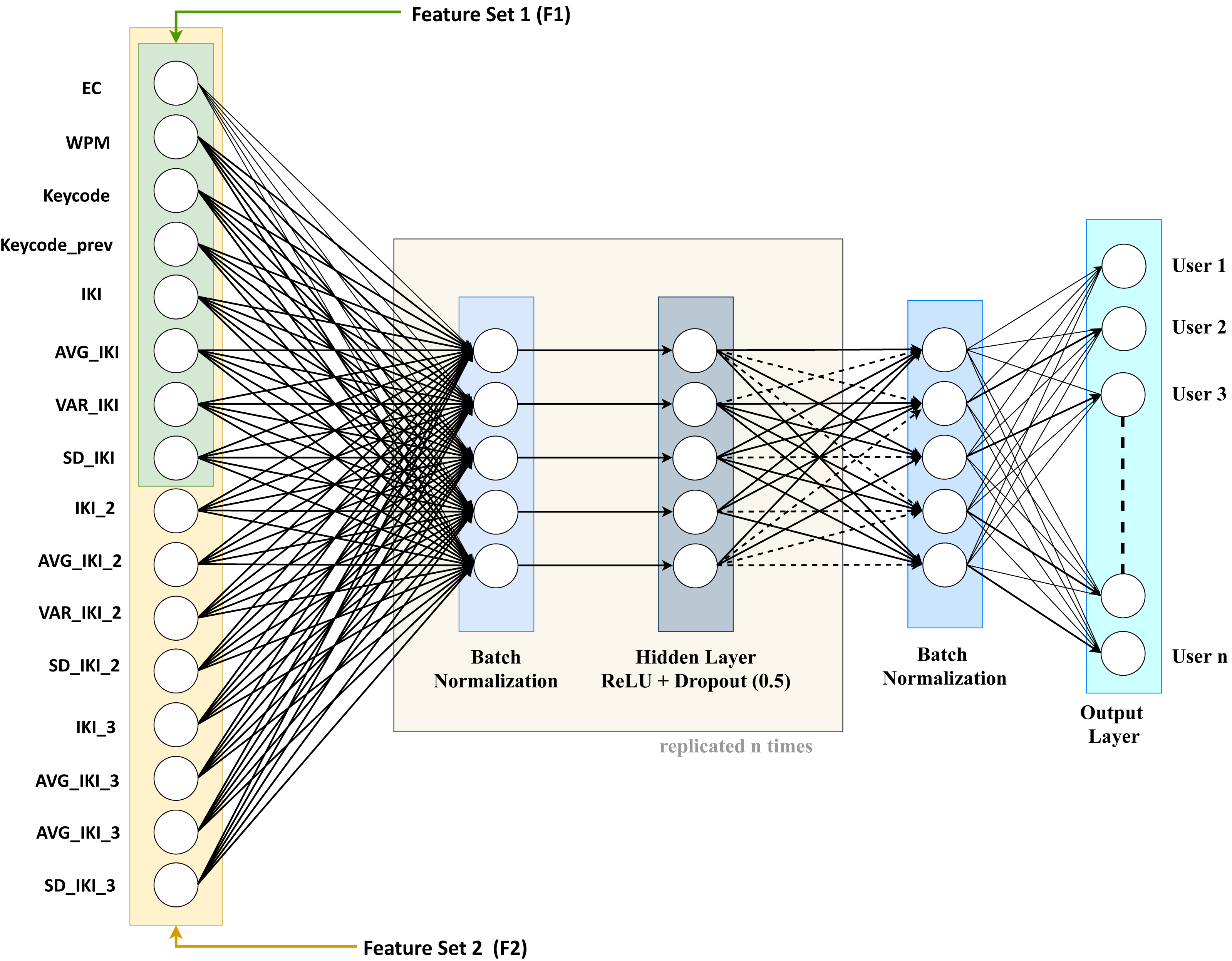
The final features set is composed of 16 features representing a user behavior along the last trigram. This permits one to understand if the inter-key interval values for the trigrams flow allow the capture of the typing behavior of the users and their better discrimination. Indeed, the complete list of the considered features is reported in the first column of Table 2. In the table, we also detailed, in the last column, the membership (black filled-in small circle) or not (empty small circle) of each feature to the integrated dataset F. The proposed feature set (F2) has been validated in a previous study (Bernardi et al., 2019), showing better outcomes than another feature set (F1) composed of only 8 features.
| Feature | DT1 | DT2 | DT3 | F |
|---|---|---|---|---|
| KEYCODE | contained | contained | contained | • |
| KEYCODE_PREV | computed | contained | contained | • |
| KEY PRESS TIME | useful | not useful | contained | ∘ |
| KEY RELEASE TIME | useful | not useful | contained | ∘ |
| IKI | computed | contained | contained | • |
| SD_IKI | computed | contained | computed | • |
| AVG_IKI | computed | computed | computed | • |
| VAR_IKI | computed | computed | computed | • |
| IKI_2 | computed | computed | computed | • |
| SD_IKI_2 | computed | computed | computed | • |
| AVG_IKI_2 | computed | computed | computed | • |
| VAR_IKI_2 | computed | computed | computed | • |
| IKI_3 | computed | computed | computed | • |
| SD_IKI_3 | computed | computed | computed | • |
| AVG_IKI_3 | computed | computed | computed | • |
| VAR_IKI_3 | computed | computed | computed | • |
| WPM | computed | contained | contained | • |
| EC | computed | computed | computed | • |
Hierarchical multiple classifier
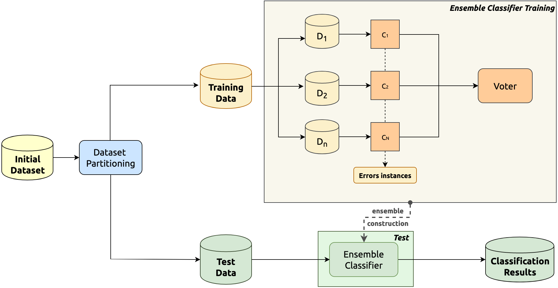
The classification methodology adopted in this paper is based on a hierarchical multiple classifier schema, depicted in Fig. 2, wherein the training phase is in the upper part, whereas the classification phase is in the lower one.

Figure 2: Overview schema of the considered hierarchical multiple classifier.
In the upper part of the figure, the partitioning procedure of the training phase is detailed. As a matter of fact, in this phase, data are partitioned into sub-datasets (D1, …Dn). In particular, the initial dataset is split into a set of data clusters which represent a sub-population of the initial training data. The splitting is performed by ensuring that each class is included in h sub-datasets, where h is an odd number at least equal to three (to allow for the majority voting during classification). Two different strategies for the class distribution into the clusters are evaluated in this paper: (i) the random and (ii) the K-means cluster data allocation strategy. The former consists in randomly choosing the classes associated with each sub-dataset; conversely, the latter entails a K-means clustering algorithm to group in the same sub-dataset all the closest classes (Coates & Ng, 2012). Specifically, we applied this algorithm to the centroids of the observations of each class. This allows one to group the classes into K clusters in which the elements of a single cluster represent the classes whose observations are allocated to a certain sub-dataset.
Each obtained sub-dataset (D1, D2, …DN) is then used to train a single basic component classifier. The set of considered basic component classifiers (C1, C2, …CN) is reported in Fig. 2 as well. Each classifier is also designed to classify as “error instances” all the instances belonging to classes not used to train the classifier itself.
Finally, an ensemble super-classifier is constructed by combining all the basic component classifiers and allowing them to vote. The ensemble super-classifier is based on a voting approach exploiting the results of the single component classifiers previously designed. The error instances generated by the component classifiers are ignored by the ensemble super-classifier.
During the test phase, for an unknown data instance, the basic component classifiers are applied to it to produce the inputs for the super-classifier (voter). The final result is produced by the ensemble super-classifier according to the input and the considered voting approach. The voting is performed by using two different approaches: (i) a simple majority voting system and (ii) a Bayesian network-based voting system.
Basic DNN component classifier
As regards the basic component classifiers of the ensemble, we considered a DNN model like the one shown in Fig. 3.
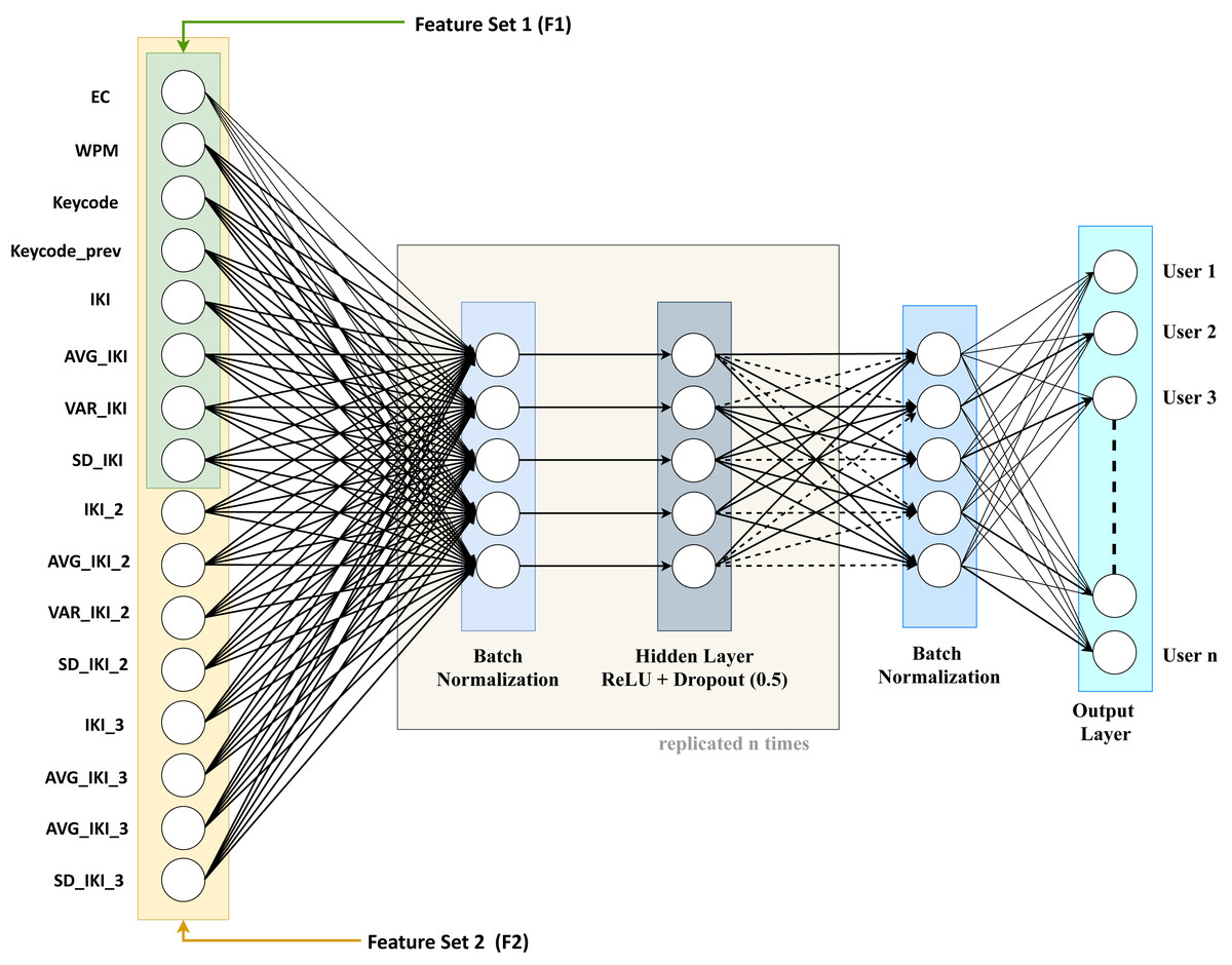
Figure 3: The considered basic DNN classifier for user identification.
The architecture of the considered basic DNN exhibits the following layers:
-
Input layer: the entry point of the considered neural network, composed of one node for each of the 16 features we described previously;
-
n sequences of three layers: the sequence is made up of a batch normalization layer, a proper hidden layer, and a dropout layer. These layers are tightly coupled and will be replicated n times in the experiments we carried out. More in detail, the three layers of the series are the following:
-
the batch normalization layer (Ioffe & Szegedy, 2015), added to improve the training process by means of speed improvements, the usage of better learning rates, and more flexibility in the initialization of the hyper-parameters. These in turn foster a more stable gradient propagation in the network leading to higher accuracy for both validation and test.
-
the actual hidden layer, made up of a variable number of “perceptrons”, decreasing from the layer closer to the input towards the layer closer to the output. The output of each perceptron of the hidden layer is a weighted sum of its inputs and is processed through a non-linear function called “activation function” (e.g., a ReLu, a sigmoid, or a soft-plus function).
-
The dropout layer, used for regularization purposes, by reducing the model complexity with a random deactivation of some perceptrons according to a Bernoulli distribution with a given p probability. In our experiments, we used 0.5 as “drop” probability.
-
-
a final batch normalization layer: used to improve the training of the output layer.
-
Output layer: this layer produces the final classification. In this work, we employed a dense layer wherein every node in input is linked to every node in the output.
The DNN architecture we considered was trained by exploiting cross-entropy (Mannor, Peleg & Rubinstein, 2005) as a loss function, whose optimization is achieved by means of a Stochastic Gradient Descent (SGD) technique. In particular, as regards SGD, we adopted a momentum of 0.08 and a fixed decay of 1e−6. In order to improve the learning performance, SGD was also integrated, in all experiments, with Nesterov Accelerated Gradient (NAG) correction to avoid excessive changes in the parameter space (Sutskever et al., 2013). During the training step, we tested architectures configured with an increasing number of hidden layers (n), in order to find out the best possible performance.
Evaluation
In this section, the evaluation setting, the considered datasets, and the results we obtained are described.
Setting
The validation is carried out by using the hierarchical multiple classifier, composed of a set of basic DNN classifiers, on the feature model previously described.
The basic DNN classifiers are trained for a changing number of layers as well as for a varying number of epochs. The latter represents a hyper-parameter which shows how many times the training is performed on the whole training dataset. The basic deep neural network classifier was implemented using Tensorflow (https://www.tensorflow.org/), an open platform for machine learning tasks, and Keras (https://keras.io/), an open-source neural network library written in Python. Similarly, the hierarchical multiple classifier was developed using the Python programming language. Different numbers of clusters (or classifiers) and different numbers of users per cluster have been evaluated along this experimentation. Finally, the multiple classifier has been evaluated by considering two different voting approaches: a simple majority vote and a Bayesian network-based vote.
The metrics used to evaluate the training performance are the Accuracy and the Loss. The loss function used is, as already stated, the cross-entropy and gives information on how well the dataset is modeled by the network. High values of loss mean that the predictions are totally wrong. On the other hand, if the loss is low, the prediction is performing well.
As regards the classification results, they were evaluated using the following metrics: Accuracy, F1 score, and ROC Area.
The accuracy is defined as follows: (11) where tp means true positives (the number of relevant retrieved instances), tn means true negatives, fn means false negatives (the number of not retrieved relevant instances), and fp means false positives (the number of irrelevant retrieved instances).
The F1 score is the weighted harmonic mean of precision and recall, which, in turn, are computed according to the following formulas: (12) (13)
Finally, the ROC (Receiver Operating Characteristic) Area (or AUC—Area Under the ROC Curve) measures the probability that a relevant instance randomly selected is classified above a not relevant one. This graph, drawn as a function of the sensitivity (or True Positive Rate—TPR) and of the specificity (or False Positive Rate—FPR), is important also because the higher the area under the curve, the higher the measure of accuracy.
To perform a comparison with other state-of-the-art (SOTA) methods, the classic Equal Error Rate (EER) metric was adopted as well. It represents the error value when the percentage of times that an imposter is erroneously identified as a legitimate user is equal to the percentage of times that a legitimate user is wrongly identified as an imposter.
The experiments were performed by using an Intel Core i9 7920X (12 cores), with RAM of 16GB and 4 GPUs (NVIDIA Titan Xp).
Dataset
Based on the study of the literature, we observed that a high number of ad-hoc datasets have been recently built, mainly to evaluate specific keystroke biometric approaches. Since these datasets are quite small and not easy to compare, they are not useful to evaluate the existing approaches. This consideration drove our idea to generate a new dataset as an integration of some existing ones. This should be useful to overrun the limitations discussed above and may support the study and the comparison of the different approaches, promising also a generalization of the obtained research results. The integration process, proposed in this study, has been developed to combine different existing datasets into a new one consistent with the feature model we designed and with the features available in each source datasets. The obtained integrated dataset is a larger one, suitable to perform the validation of our proposed approach. The integration process consists of the following main steps:
-
the evaluation of each dataset according to the designed feature model;
-
the cleaning and filtering of the datasets;
-
the specification of the data transformation rules;
-
the merging of the datasets.
The first step allowed the evaluation of all the features in each initial input dataset to assess their suitability according to the designed feature model.
In the following step, the input datasets are cleaned by filtering all the unnecessary information.
In the third step, for each input dataset, some processing modules were added to specify the logic used to transform (or evaluate when needed) the source features into the target features.
The cleaned and transformed datasets were then combined in the last step.
The integration process we devised is designed to ensure an easy and iterative extension of the integrated datasets, by adding new transformation rules for each newly added dataset, and it was written in Python language.
In this study, we integrated three datasets (DT1, DT2, DT3) whose statistics and features, referred to the designed feature model, are reported in Tables 3 and 2, respectively. The selection of the datasets was performed by considering the following criteria: (i) the data acquisition process has to be meticulous, repeatable, and well documented; (ii) the dataset subjects have to be widely varied in terms of samples per user as well as regarding the particular typing scenario; (iii) the information contained in each dataset has to be compatible, to a certain extent, to the designed feature model.
| Dataset | #Users | #Samples per user | Samples size | Reference |
|---|---|---|---|---|
| DT1 | 1500 | 4 | 954.82 | Banerjee et al. (2014) |
| DT2 | 30 | ≈1200 | 89.65 | Feit, Weir & Oulasvirta (2016) |
| DT3 | 168000 | 11.25 | 48.85 | Dhakal et al. (2018) |
For all considered datasets, Table 3 shows the number of users, the samples per user, the sample size (evaluated as the average number of characters per sentence), as well as the corresponding reference. Looking at the first row, in DT1 there are 1,500 users and four sentences are typed by each user. The sentences have various lengths (the average length of the sentences is 955 characters and there is no sentence with less than 100 characters). In the second row of the table, DT2 contains the data of 30 users and each user types ≈1200 small sentences (the average length is about 90 characters). Finally, in the last row of the table, the description of dataset DT3 is reported. It contains data from about 168,000 users. Each user types about 11 small sentences (the average length is 49 and the largest sentence is composed of 141 characters). The data were collected via an online typing test published as a part of a free typing speed assessment Web page.
Table 2 highlights, for all the datasets, if a considered feature is: (i) already contained in it (contained); (ii) useful to calculate other features (useful); (iii) not useful to calculate other features (not useful) and (iv) computed by using existing features (computed). Filled-in circles indicate features considered in the final integrated dataset, while empty circles characterize features not being present in the final integrated dataset, which is available online at this link (https://doi.org/10.6084/m9.figshare.14066456).
Training results
In this subsection, we discuss some results obtained from the execution of the training process of both the basic component classifier and the ensemble super-classifier.
The basic neural networks are trained by changing the number of epochs and layers. The number of epochs should be set to ensure the best performance of the network. This is obtained when the network accuracy trend becomes approximately stable. The time to reach a stable condition is related to the learning rate, a hyper-parameter that defines to what extent newly acquired information overrides old information, which was varied to find its best-performing value.
The plots depicted in Figs. 4 and 5 show the accuracy and the loss for a set number of layers (ranging from 6 to 9) versus an increasing number of epochs in the training phase of the basic component neural network (the figures depict for each considered layer the best learning rate). Looking at Fig. 4, we can observe that in all cases the obtained accuracy after 100 epochs is higher than 90%. The worst accuracy is obtained when the number of layers is 9; indeed, in this case, the curve starts well, but when it reaches saturation (about after 100 epochs) its performance tends more and more slightly to become the worst one. The best curve is for almost all the epochs the one of the 8-layer classifier, but if we observe carefully the trends in the end (about after 300 epochs), the accuracy value of the 7-layer classifier is the closest to 1, thus resulting in the best configuration. Finally, the 6-layer classifier exhibits always an intermediate trend, compared to the other curves.
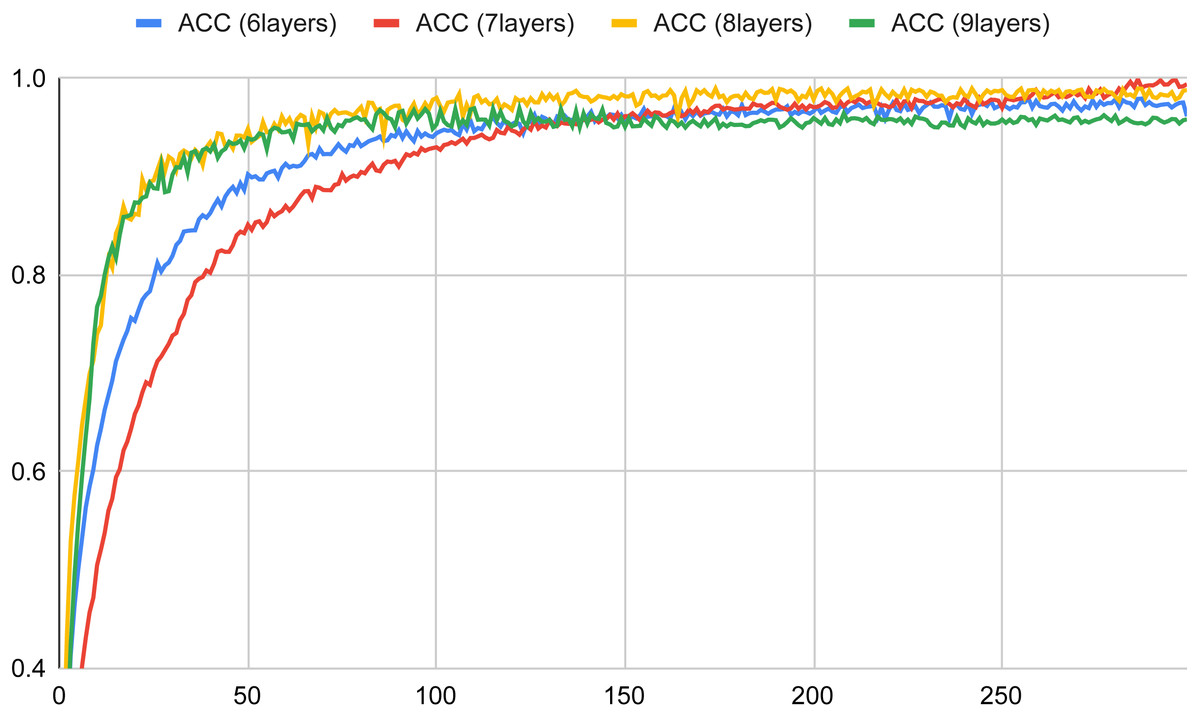
Figure 4: Accuracy versus the number of epochs with six, seven, eight and nine layers for the basic neural network (in a typical training session).
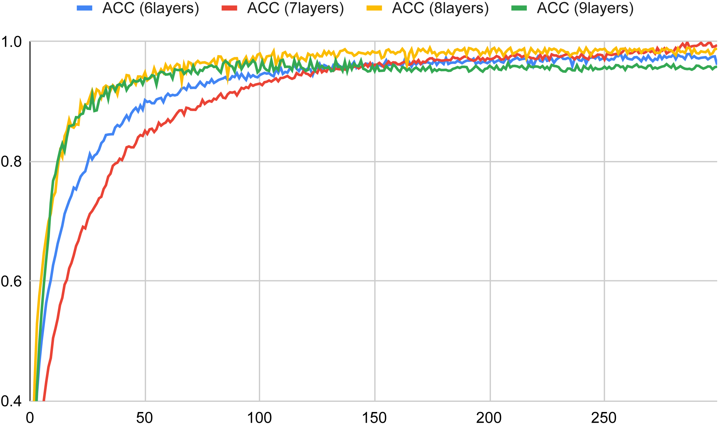
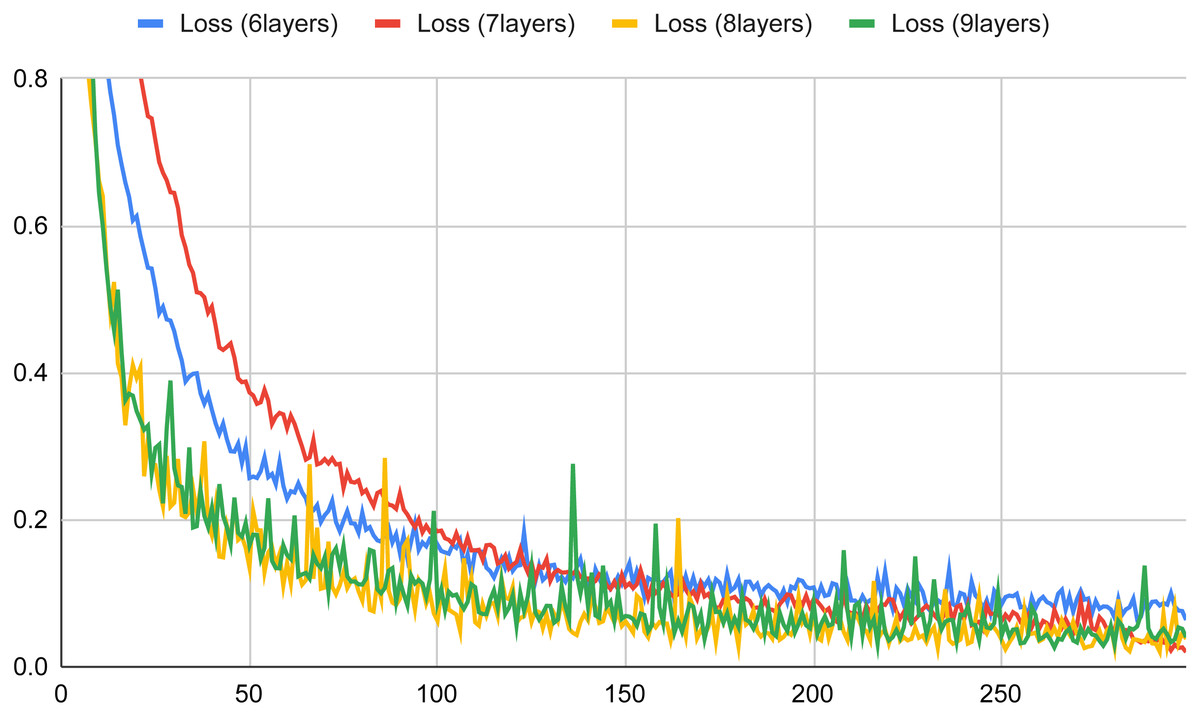
Figure 5: Loss versus the number of epochs with six, seven, eight and nine layers for the basic neural network classifier (in a typical training session).
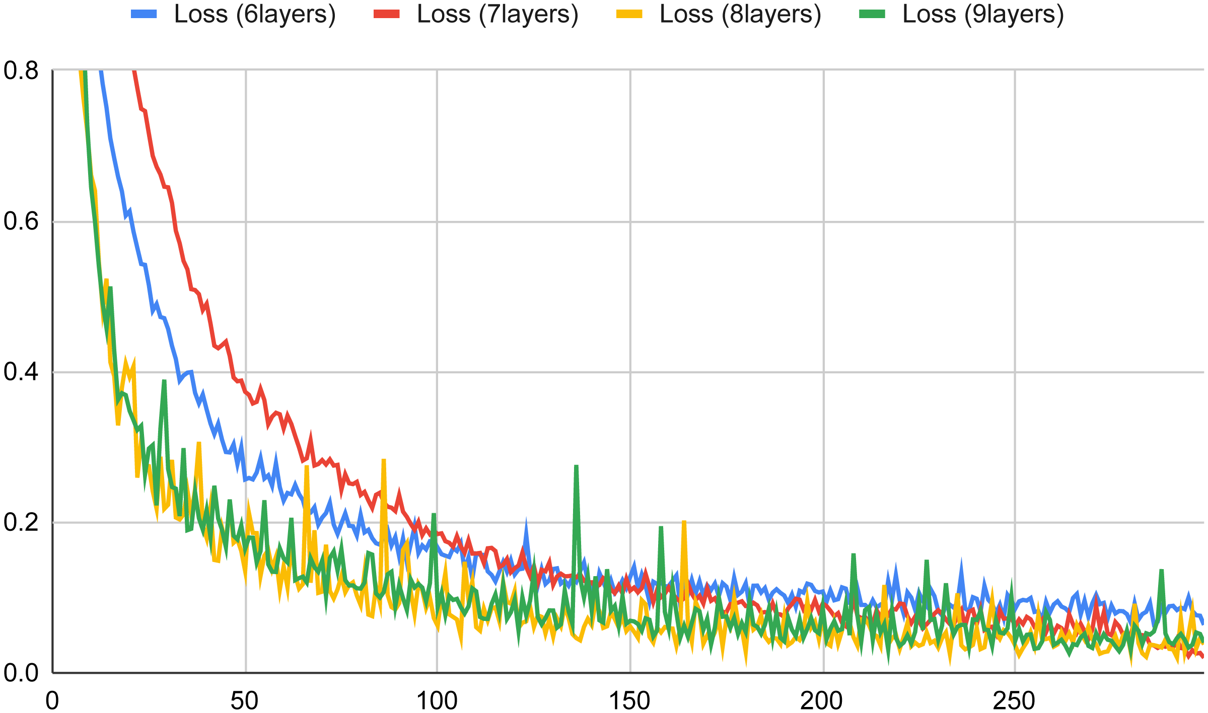
Similar, but symmetrical, considerations can be inferred from Fig. 5 regarding the loss values. In this case, for all the considered layers, we obtained loss values very close to zero, and the best results are obtained when the number of layers is 7 and the number of epochs is closer to 300.
Given the above considerations, we considered, in the following evaluation of the hierarchical multiple classifier, basic classifiers composed of neural networks endowed with 7 layers, since this configuration provides the best possible performance.
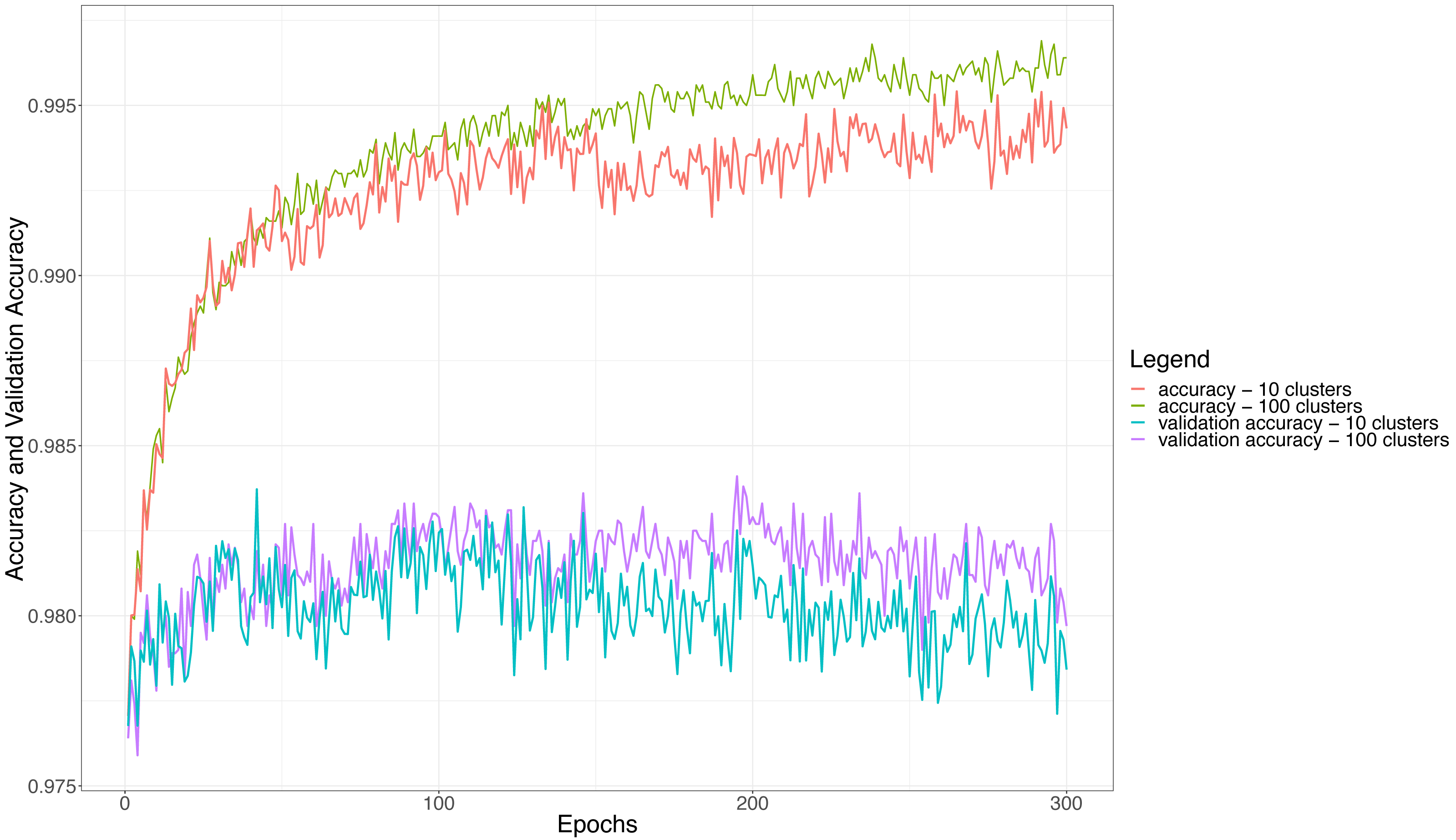
Concerning the hierarchical multiple classifier, some other considerations can be made about the number of adopted clusters, since the clustering strategy may affect both accuracy and loss during the training of the ensemble itself. Figure 6 shows the accuracy and validation accuracy obtained for the hierarchical multiple classifier when we set the number of clusters to 10 (100 users per classifier) and 100 (10 users per classifier), respectively. The figure shows that the best values of accuracy are obtained when the number of clusters is 100, this confirms the intuition that the fewer the users to be discriminated by each basic classifier (more clusters means fewer users per cluster), the higher the performance of the classifier itself and so the performance of the whole ensemble. The figure shows that the accuracy becomes almost constant when the number of epochs is more than 250: this means that after about 250 epochs the whole ensemble will not be learning anymore and the accuracy will not become higher. Similar observations can be made for the validation accuracy, i.e., the accuracy calculated for the validation dataset; however, in such a case, the threshold after which the accuracy tends to stabilize amounts to about 100 epochs. It is also worth noting that the validation accuracy curves are always lower than the corresponding accuracy curves, even if the difference, at most, is about 1.25%, dropping from about 99.5% to 98.25%. This indicates that the validation on a never-seen dataset is anyway high performing.
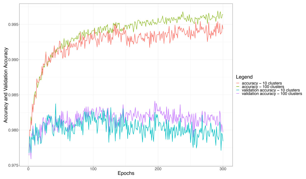
Figure 6: The accuracy and the validation accuracy for the whole ensemble classifier with 10 and 100 clusters (in a typical training session).
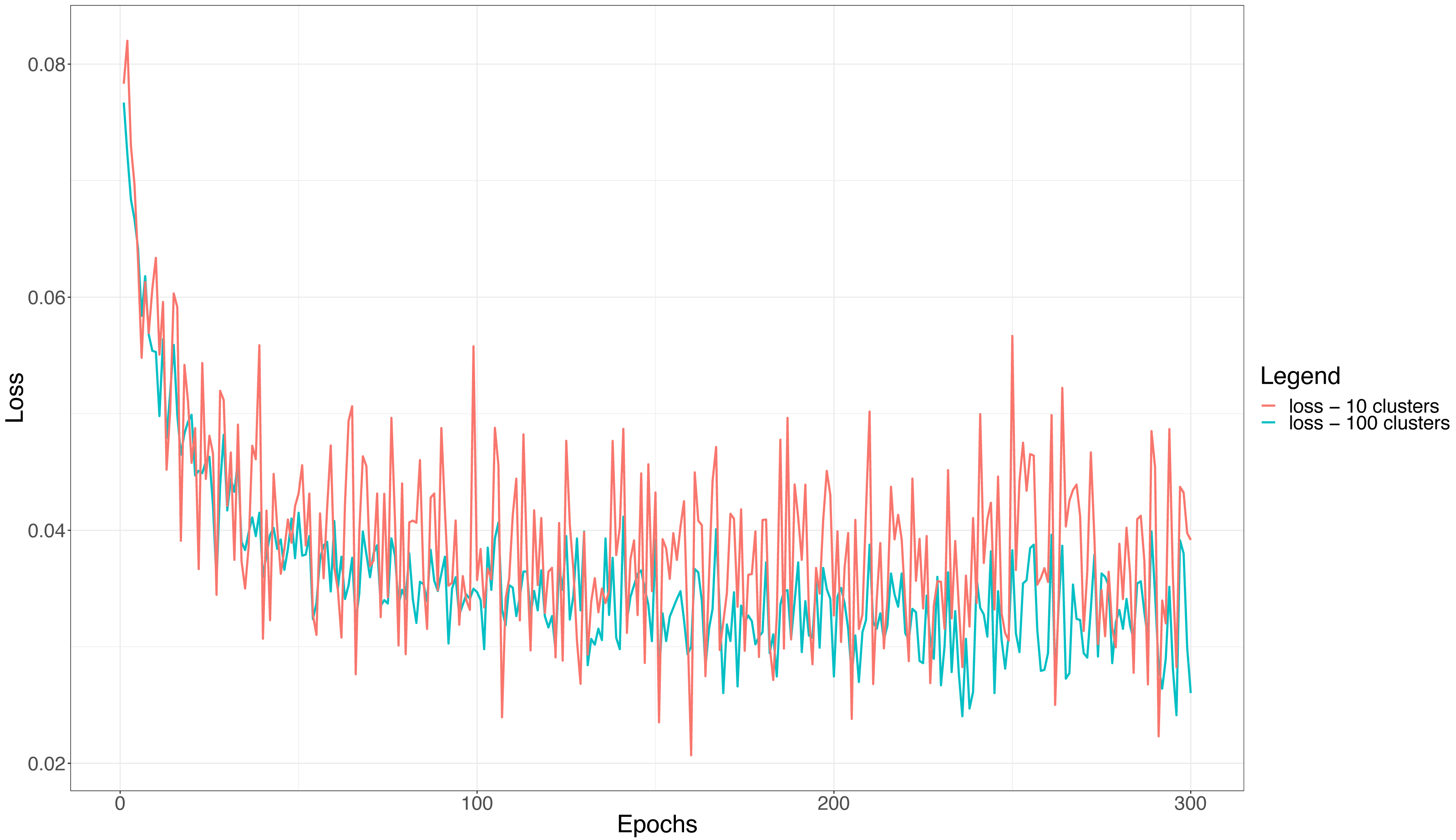
Similar, but symmetrical, trends are experienced by the loss curves reported in Fig. 7. The figure highlights that the curves are noisier whenever the number of clusters is 10, i.e., we need to discriminate 100 users per basic classifier. This corroborates further the above considerations, that is, a larger number of users per cluster (classifier) makes the overall classification of the ensemble more difficult and unstable. Finally, as it is the case with the accuracy, when the loss becomes constant the network does not learn anymore. This happens, in the case of the loss, after almost 150 epochs, thus a little earlier than when the accuracy curves reach saturation, but consistently with the validation accuracy curves.
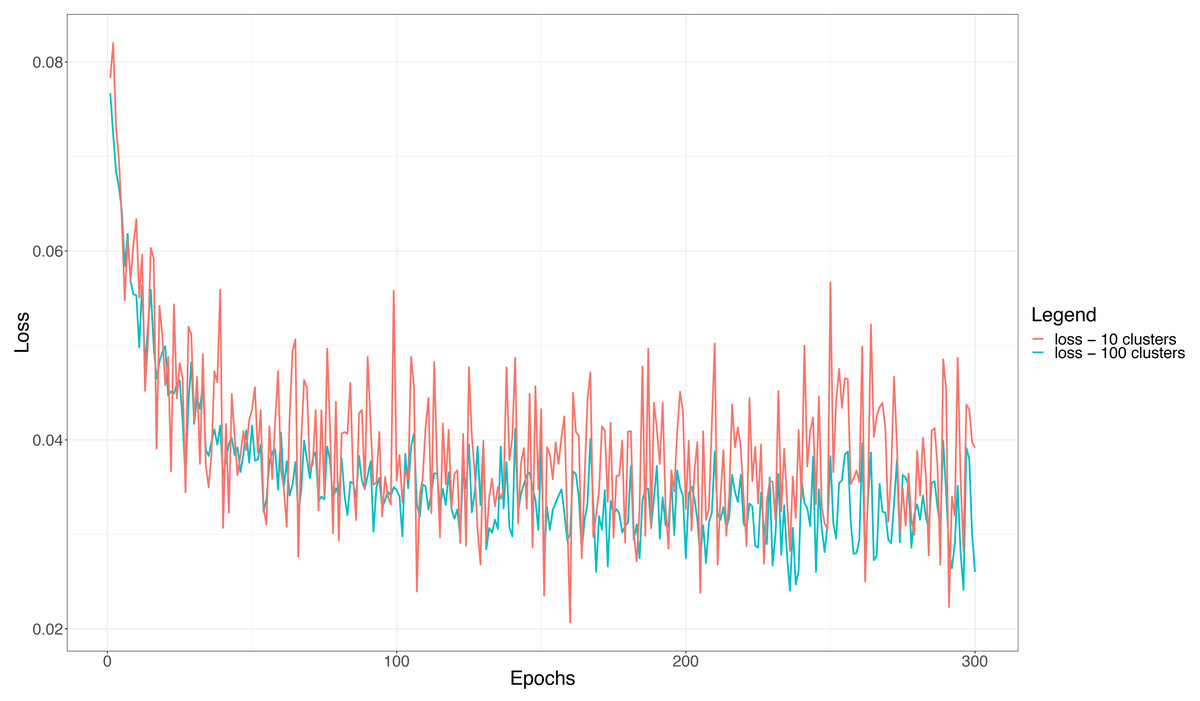
Figure 7: The training loss function for the ensemble classifier with 10 and 100 clusters in a typical training session.
Classification results
This subsection describes the results we achieved during the classification phase on the test set. Table 4 shows the accuracy obtained considering different combinations of (i) the number of clusters (first column), (ii) the number of users per cluster (second column) (iii) the allocation method of the users to the clusters (third column), (iv) the voting method of the ensemble super-classifier (fourth column), and (v) the number of epochs (fifth column). The numbers of clusters we considered are 100, 50, 20, and 10, respectively. The evaluation is performed by considering 1,000 users that are equally distributed on each cluster (for example, if the number of considered clusters is 100 the number of users per cluster is 10).
| Number of clusters | Users per cluster | Allocation method | Voting method | Epochs | Accuracy |
|---|---|---|---|---|---|
| 100 | 10 | Random | Majority | 100 | 0.972 |
| Majority | 200 | 0.988 | |||
| Majority | 300 | 0.994 | |||
| Bayesian | 100 | 0.980 | |||
| Bayesian | 200 | 0.984 | |||
| Bayesian | 300 | 0.995 | |||
| K-means | Majority | 100 | 0.971 | ||
| Majority | 200 | 0.985 | |||
| Majority | 300 | 0.991 | |||
| Bayesian | 100 | 0.984 | |||
| Bayesian | 200 | 0.988 | |||
| Bayesian | 300 | 0.997 | |||
| 50 | 20 | Random | Majority | 100 | 0.939 |
| Majority | 200 | 0.966 | |||
| Majority | 300 | 0.984 | |||
| Bayesian | 100 | 0.945 | |||
| Bayesian | 200 | 0.957 | |||
| Bayesian | 300 | 0.987 | |||
| K-means | Majority | 100 | 0.920 | ||
| Majority | 200 | 0.958 | |||
| Majority | 300 | 0.976 | |||
| Bayesian | 100 | 0.957 | |||
| Bayesian | 200 | 0.971 | |||
| Bayesian | 300 | 0.993 | |||
| 20 | 50 | Random | Majority | 100 | 0.953 |
| Majority | 200 | 0.974 | |||
| Majority | 300 | 0.978 | |||
| Bayesian | 100 | 0.964 | |||
| Bayesian | 200 | 0.964 | |||
| Bayesian | 300 | 0.990 | |||
| K-means | Majority | 100 | 0.934 | ||
| Majority | 200 | 0.969 | |||
| Majority | 300 | 0.984 | |||
| Bayesian | 100 | 0.973 | |||
| Bayesian | 200 | 0.978 | |||
| Bayesian | 300 | 0.994 | |||
| 10 | 100 | Random | Majority | 100 | 0.906 |
| Majority | 200 | 0.952 | |||
| Majority | 300 | 0.976 | |||
| Bayesian | 100 | 0.894 | |||
| Bayesian | 200 | 0.942 | |||
| Bayesian | 300 | 0.982 | |||
| K-means | Majority | 100 | 0.868 | ||
| Majority | 200 | 0.940 | |||
| Majority | 300 | 0.965 | |||
| Bayesian | 100 | 0.930 | |||
| Bayesian | 200 | 0.959 | |||
| Bayesian | 300 | 0.990 |
The allocation methods we evaluated are random or K-means, while the only considered voting methods are majority and Bayesian. Finally, three different numbers of epochs, namely 100, 200, and 300, were considered, in order to encompass the most significant values found out in the training process of both the single and the ensemble classifiers.
The table shows that for all the considered combinations the obtained accuracy values are always greater than 0.868 (this value is obtained when the number of clusters is set to 10, adopting the K-Means algorithm and the majority voting, and considering 100 epochs). However, the overall average value, across all the combinations, of the obtained accuracy is 0.965, which is a very good result on average. Furthermore, the best accuracy (0.997, in bold in the table) was obtained when the number of clusters is set to 100, the K-Means algorithm as well as the Bayesian voting system are adopted, and 300 epochs are considered. The results of the table confirm that smaller clusters permit a better overall performance and that applying either K-Means or random distribution methods leads to very similar outcomes (the average accuracy values are 0.966 and 0.965, respectively).
By the same token, the two different voting methods (majority or Bayesian) produce 0.960 and 0.970 as average accuracy values, indicating a light advantage of the Bayesian voting method.
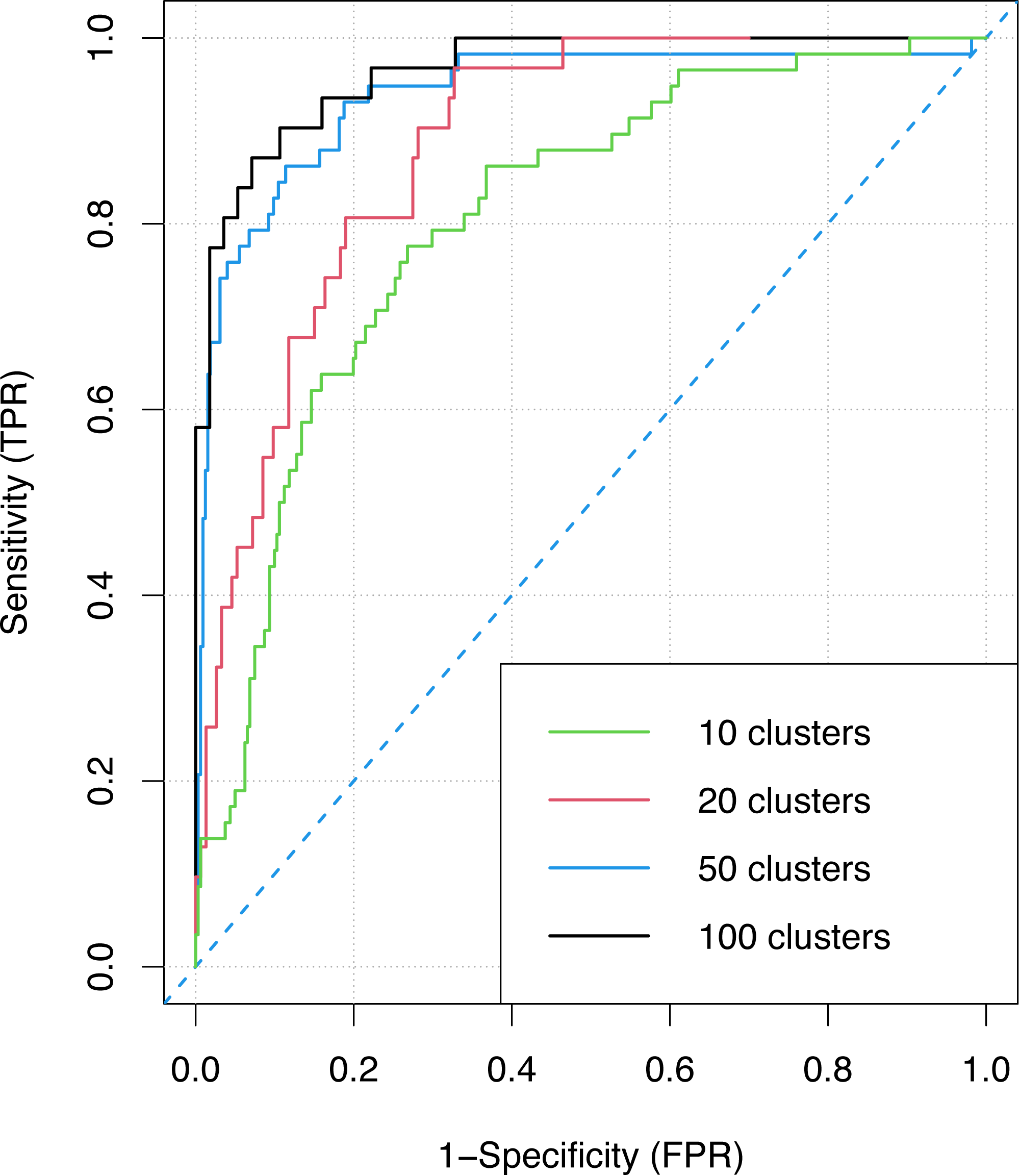
Finally, Fig. 8 shows the ROC curve of the ensemble classifier obtained with an increasing number of clusters (10, 20, 50, 100) when the best on average allocation and voting methods are employed, i.e., K-means clustering and Bayesian voting. The figure demonstrates that the ensemble super-classifier exploiting 100 clusters has the best measure of separability (AUC = 0.991 and F1 = 0.98) and the best accuracy, given that the higher the area under the curve, the higher the measure of accuracy. This confirms, even more, the considerations already drawn previously regarding the fact that choosing small clusters is the best performing choice. On the other hand, the worst values are obtained when the number of clusters is 10 (AUC = 0.957 and F1 = 0.97), i.e., when the basic classifiers have to deal with 100 users each. Notwithstanding, also in this worst case the results are good in the context of deep learning techniques.
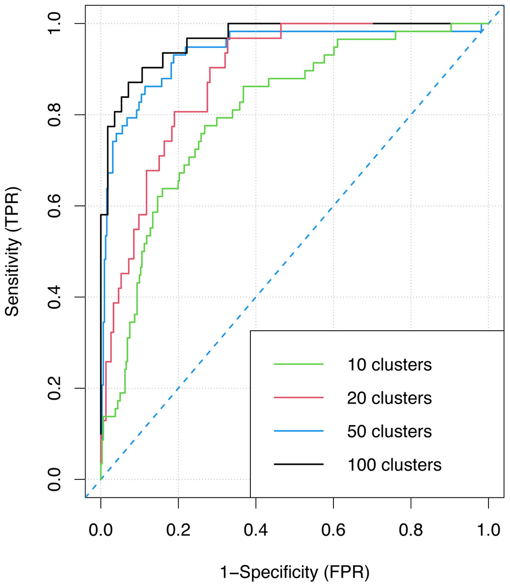
Figure 8: The ROC curve for the ensemble classifier with different numbers of clusters.
In order to provide an indication of the performance of the proposed approach in comparison with those proposed in recent years, we calculated also the value of the EER with and without ensemble and for different numbers of users involved. In Table 1, presented in the second section of the manuscript, for each comparable approach, the value of the best EER (last column) is reported. It is worth noting that the proposed approach for 100 users, without using dataset partitioning and ensemble, is still able to provide acceptable performance with respect to other SOTA methods. Above one hundred users and up to one thousand, our ensemble approach provides the same level of performance with small degradation. We cannot perform a comparison with other SOTA methods in terms of performance for more than one hundred users since this information, although interesting, is not available. Finally, since Table 1 shows that the only approach that provides better results than our solution, in terms of EER, is the one proposed in Porwik, Doroz & Wesolowski (2021), we can say that, differently from this work, this performs intrusion detection using binary classification and is not able to identify the typing user within a large dataset.
Threats to the Validity of the Study
This section discusses the main threats to the validity of our research.
Construct validity threats concern the relationship between theory and observation, i.e., whether there could be some oversights and omissions in the measurements. A possible discussion about the construct validity has been briefly discussed previously when the EC feature has been introduced. Specifically, this metric does not include all the possible correction events, but we only focused on the events that can be easily extracted from the available datasets. Moreover, we adopted a “blind” notion of error since the correct text the user is typing is not always known. In order to avoid such limitations in the applicability of the approach, we only considered the errors that required an explicit action by the user (i.e., explicit deletes with “cancel” and “backspace” keys). Considering it within these limits, the EC can still be considered as being significantly representative of the error frequency of the typing user and the obtained results confirm that it is highly discriminating.
A further possible construct validity may regard the computation of the typing speed in the form of words per minute. As a matter of fact, it may be tricky to estimate it in case no transcription tasks are performed by the users. In the considered data, two out of three datasets appear to be keyboard interactions recorded during transcription tasks, so the computation of timing-related features is simplified. In future developments, it could be devised a proper methodology to measure time-related features also in typing scenarios with many pauses.
Internal validity threats concern those factors being able to influence our observations. In this study, an internal validity threat is represented by the fact that we considered in our experiment some existing labeled datasets: if the typing is not correctly associated with the users or the datasets are not obtained with a rigorous process, we could have classification errors. This risk is strongly mitigated because the selected datasets are well documented and referenced.
Threats to external validity concern the generalization of our findings in real-world typing. We have assessed our approach on a 169,530-user dataset from three existing datasets having different sizes, characteristics, and previously adopted with different goals. This represents a novelty with respect to similar studies that are mainly based on ad-hoc built datasets.
However, as already stated, two out of three datasets appear to be keyboard interactions recorded during transcription tasks, while in other real-world typing scenarios people constantly pause during periods of typing, perhaps due to thinking about what to type next, switching back and forth between different programs, drifting attention because of everyday life distractions, etc.
Moreover, we have only considered data from the physical keyboard of an actual desktop computer, which could be quite different from those derived from “virtual” keyboards on mobile devices.
At any rate, in the future, it is possible to further integrate more datasets coming from more real-world typing scenarios, allocating different typing behaviors to different basic classifiers, to be optimized separately one from the other.
Finally, our evaluation is performed on clusters of a maximum of one thousand users from the complete dataset, assessing the ensemble performance only in this range. In order to generalize the performance on a larger number of users (more than one thousand), further experiments need to be performed.
Conclusion and Future Work
This paper proposes an innovative approach that aims at discriminating many users on the basis of their typing dynamics. The approach considers a group of 16 unique features used for training a hierarchical multiple classifier exploiting single basic deep neural networks. A large dataset was constructed in order to validate such an approach, through the integration of three real-world existing datasets. First, we have optimized a basic classifier implemented as a deep neural network, and then we have built a hierarchical multiple classifier with different strategies for allocating users and various strategies for the final voting procedure. We have achieved the best performance when K-Means is used for user allocation and Bayesian voting is employed for the final decision: this configuration leads to a very promising overall accuracy of 0.997.
This study has multiple future developments that can be addressed. The first is to verify the possibility of integrating new features into the existing dataset. This is a preliminary step that will provide us the possibility to evaluate how to extend our investigation and how to obtain an even larger dataset.
Moreover, we plan to test other allocation strategies and other voting techniques, such as stacking, comparing them to identify the best-performing ones. Finally, Process Mining techniques (Bernardi et al., 2014) will be considered to identify users even using a higher-level behavioral model.