
Topological insights and hybrid feature extraction for breast cancer detection: a persistent homology classification approach
- Published
- Accepted
- Received
- Academic Editor
- Davide Chicco
- Subject Areas
- Computer Vision, Data Mining and Machine Learning
- Keywords
- Breast cancer classification, Topological data analysis, Persistent homology, Computer vision
- Copyright
- © 2025 Jetomo et al.
- Licence
- This is an open access article distributed under the terms of the Creative Commons Attribution License, which permits unrestricted use, distribution, reproduction and adaptation in any medium and for any purpose provided that it is properly attributed. For attribution, the original author(s), title, publication source (PeerJ Computer Science) and either DOI or URL of the article must be cited.
- Cite this article
- 2025. Topological insights and hybrid feature extraction for breast cancer detection: a persistent homology classification approach. PeerJ Computer Science 11:e3374 https://doi.org/10.7717/peerj-cs.3374
Abstract
Early detection of breast cancer by mammography scans is crucial for improving treatment outcomes. However, low image resolutions, size, and location of lesions in dense breast tissue prove to be challenges in mammography, underscoring the importance of accurate and efficient computer-aided diagnostic systems. This article introduces a novel classification framework that utilizes histogram of oriented gradients (HOG) as a feature extractor and principal component analysis (PCA) for dimensionality reduction. Classification is implemented using the persistent homology classification algorithm (PHCA), which leverages persistent homology (PH) to capture topological properties of mammography images. The framework was evaluated on 7,632 images from the INbreast dataset with an extensive use of grid-search cross-validation to optimize preprocessing parameters. Two optimal combinations of HOG parameters and scaler were identified, with the best configuration (16 × 16 pixels per cell, 3 × 3 cells per block, and Minmax scaler) achieving strong performance. Validating on the test set, PHCA achieved an overall accuracy, precision, recall, F1-score, and specificity of 97.31%, 96.86%, 97.09%, 96.97%, and 96.86%, respectively. Clinically, the high precision (98.23%) and high recall (97.75%) for malignant cases highlight PHCA’s sensitivity in identifying malignancies, ensuring that very few malignant cases go undetected with highly trustworthy predictions. These results are shown to be competitive with existing state-of-the-art models, even exceeding in some cases, while requiring lower computational cost than deep learning-based approaches. Although the proposed method trails advanced deep models by 3–4% in some metrics, it offers a computationally efficient alternative and a potential for deployment in large-scale screening systems, demonstrating the promise of topological data analysis for breast cancer classification.
Introduction
Breast cancer remains one of the most widespread health problems in the world, with millions of new cases diagnosed every year. According to the American Cancer Society, over 310,720 women in the United States will be diagnosed with invasive breast cancer in 2024, and approximately 56,500 cases of ductal carcinoma in situ (DCIS) are predicted (American Cancer Society, 2024). It accounts for nearly 30% of all new cancer cases diagnosed in women each year. The incidence of breast cancer is highest in middle-aged and older women, with an average age at diagnosis of 62. While breast cancer is less common in younger women, a small percentage is diagnosed before the age of 45.
Early detection remains the cornerstone of effective breast cancer treatment. Numerous studies emphasize its importance in reducing mortality and improving survival rates (Wang, 2017). Early detection usually involves screening procedures such as mammography, which can detect breast cancer at a much earlier stage, before symptoms appear. If the disease is detected before it metastasises, the prognosis improves significantly (Wrubel, Natwick & Wright, 2020; Elmore et al., 2005).
Mammograms offer several advantages in detecting early signs of breast cancer, yet radiologists face challenges such as low image resolution, lesion size and location, and dense breast tissue (Ruza et al., 2023). These factors increase the risk of misdiagnosis, underscoring the need for accurate and efficient computer-aided diagnosis (CAD) systems. Persistent Homology (PH), a technique from Topological Data Analysis (TDA), has emerged as a promising tool for addressing these challenges.
PH has been increasingly recognized for its potential in capturing the intrinsic topological structures of complex datasets. By analyzing the shapes and structures of data points in high-dimensional spaces, PH provides unique insights into patterns within medical images. Applications span cardiovascular (Ren et al., 2023), musculoskeletal (Yadav, Nisha & Coskunuzer, 2023), neurology (Tan et al., 2023), ophthalmology (Chen et al., 2023), and oncology (Hahn et al., 2021; Malek et al., 2023).
Related works
Persistent Homology (PH), a core method in TDA, has gained increasing attention in medical imaging due to its ability to capture intrinsic structural features of complex data. By encoding both local and global topological properties, PH has been applied across diverse medical domains. For example, Ren et al. (2023) applied PH to ECG analysis, Yadav, Nisha & Coskunuzer (2023) to musculoskeletal imaging, Tan et al. (2023) to brain signals, and Chen et al. (2023) to retinal image analysis. In oncology, Hahn et al. (2021) studied DNA repair in breast cancer cells, while Malek et al. (2023) applied PH to mammography microcalcifications.
In breast cancer classification, Anjum et al. (2021) combined histogram of orientedgradients (HOG) and Canny edge detection with support vector machine (SVM) achieving 94% accuracy. Similarly, Mu’jizah & Novitasari (2021) integrated HOG, principal component analysis (PCA), and SVM, reporting 100% sensitivity and 97.5% specificity. These works demonstrate that hybrid methods leveraging gradient-based and topological features can enhance diagnostic performance.
Despite these advances, state-of-the-art approaches still rely heavily on convolutional neural network (CNN)-based deep learning models (El Houby & Yassin, 2021; Karthiga, Narasimhan & Amirtharajan, 2022; Jabeen et al., 2023; Yadav & Kumar, 2025), with some exploring ensemble-based learning (Shah et al., 2024; Haq et al., 2022; Batool & Byun, 2024) which, although effective, require extensive preprocessing and computational resources, limiting their scalability in real-world settings.
Research gap
To date, limited studies have systematically explored the integration of PH with hybrid feature extraction and dimensionality reduction methods for mammography classification. Existing works either focus exclusively on deep architectures (Jabeen et al., 2023; Yadav & Kumar, 2025) or apply PH in isolation without leveraging its synergy with descriptors like HOG. This leaves a gap for computationally efficient yet accurate frameworks that combine PH with conventional feature extraction to provide reliable alternatives to deep networks. Addressing this gap, our study introduces a persistent homology classification algorithm (PHCA)-based classification framework with HOG and PCA, aiming to deliver strong diagnostic performance while maintaining efficiency and scalability.
In summary, the combination of PH with hybrid feature extraction methods such as HOG and dimensionality reduction techniques such as PCA is a promising approach for breast cancer classification. These methods enable the extraction of rich topological features from high-dimensional image data, contributing to more accurate and efficient diagnostic tools. The major contribution of this study is the development of a novel breast cancer classification framework that integrates HOG for feature extraction, PCA for dimensionality reduction, and PHCA for classification. Unlike deep learning approaches, the proposed method provides competitive performance while being computationally efficient, making it suitable for large-scale screening applications. This work further demonstrates the potential of topological methods in medical image analysis, effectively bridging the gap between traditional feature-based and deep learning approaches.
Methodology
This section outlines the detailed procedure of this study, including the preparation of the dataset, feature extraction, dimensionality reduction, and the classification method used to identify breast cancer tumors in mammography scans.
Dataset
The dataset used in this article is extracted from the INbreast database, the summarized description of which is presented in Table 1. It consists of 7,632 mammogram images categorized into two classes: 2,520 benign and 5,112 malignant images from Huang & Lin (2020). The mammography images in the INbreast database were originally collected from the Centro Hospitalar de S. Joao (CHSJ) Breast Center in Porto. The database contains data collected from August 2008 to July 2010 and includes 115 cases with a total of 410 images (Moreira et al., 2012). Of these, 90 cases concern women with abnormalities in both breasts. Four different types of breast disease are recorded in the database: Mass, calcification, asymmetries and distortions. The mammograms are recorded from two standard perspectives: Craniocaudal (CC) and Mediolateral Oblique (MLO). In addition, breast density is classified into four categories based on the BI-RADS standards: Fully Fat (Density 1), Scattered Fibrous-Landular Density (Density 2), Heterogeneously Dense (Density 3) and Extremely Dense (Density 4). The images are stored in two resolutions: 3,328 4,084 pixels or 2,560 3,328 pixels, in DICOM format. A total of 106 mammograms depicting breast masses were selected from the INbreast database.
| Dataset | INbreast |
|---|---|
| Source | Centro Hospitalar de S. Joao (CHSJ) Breast Center |
| Nature | Mammography images |
| Case types | Benign, Malignant |
| # Images | 2,520 benign, 5,112 malignant |
| Dimension |
To enhance the dataset for model training, data augmentation techniques were applied. Image preprocessing method using contrast limited adaptive histogram equalization (CLAHE) was used to the 106 mammograph scans (Huang & Lin, 2020), making the lesions more detectable but may cause feature distortion. Then, multiple-angle rotation ( with increments) and image flipping were then implemented, imitating variations in breast orientation which helps the model to train on generalized acquisition angles. From these steps, the dataset is increased from 106 to 7,632 mammography images.
Each image is preprocessed to ensure a uniform size and format. In particular, all images are resized to 224 224 pixels to ensure uniformity across the dataset and converted to grayscale to reduce the computational complexity associated with multi-channel (RGB) data.
Grayscale conversion is particularly important in medical imaging. In this way, the intensity values of the images are preserved while the color information, which is not relevant for this classification task, is discarded. By focusing exclusively on the pixel intensity, the computational effort is significantly reduced without losing important information. In addition, data augmentation techniques, including image rotation, have been applied to increase the variability of the dataset. The expansion helps to prevent overfitting during model training by exposing the model to a wider range of image variations.
Feature extraction using histogram of oriented gradients
HOG is a feature descriptor used to define an image by the pixel intensity and intensities of gradients of pixels (Madhuri & Negi, 2023). It does so by computing for edges and shapes on a dense grid of uniformly spaced cells and improves its performance by using overlapping contrast normalization. Particularly, the method divides the image into a small spatial region called cell. The combination of magnitude and angle derived from each cell will be accumulated to develop the -dimensional histogram of gradients. Then, the contrast normalization is performed on the local histogram by accumulating the derived 1-dimensional histogram of gradients of each cell performed by relatively larger spatial regions called blocks. In total, three parameters are usually set for HOG, namely: dimension of a cell, dimension of a block, and number of orientations.
One of HOG’s main advantages is its robust nature in capturing local edge and shape information, effective for distinguishing structural patterns from subtle texture variations. This makes it useful specific to identifying tumors where boundary and margin details are crucial diagnostic features. However, despite HOG being easy to implement and more computationally efficient than deep learning approaches, its performance is sensitive to parameter selection. It also results with high-dimensional descriptors, requiring the need for dimensionality-reduction methods.
Algorithm of HOG
-
1.
Gradient computation
For each pixel of an image, HOG descriptor is applied. This is done by computing the horizontal and vertical gradients using the 1-dimensional kernel. Let be the ith-row and jth-column pixel of the image. For each pixel, the horizontal and vertical gradients are computed as (1) (2) From this, the magnitude G and direction of the gradient of each pixel are respectively computed as (3) (4)
-
2.
Orientation binning
After computing the gradient magnitude and direction for each pixel in the image, the image is divided over a local spatial region called cell. Suppose that the specified dimension of a cell is (note that a cell can also be a square). This means that each cell consists of rows and columns of pixels. For each cell, the gradient pixel gives a weighted vote by allocating its corresponding magnitude to bins that correspond to the direction. The vote are assigned to the center of each neighboring direction bins that are evenly spaced over to through bilinear interpolation. Increasing the direction bins provide significant increase in its performance until up to nine bins.
-
3.
Normalization and descriptor blocks
Cells will then be grouped into a larger spatial region called blocks. Local contrast normalization is implemented for each block to account for local variation in illumination and foreground-background contrast. Let be the non-normalized vector, be its -norm, and be a small constant. In this article, the L2-norm is used which implies that the normalized vector is computed as (5) The final descriptor of the image is then represented as the concatenated vector components corresponding to each normalized block. This is then used as the feature vector for each image.
Dimension reduction using principal component analysis
Principal component analysis (PCA) aims to take high-dimensional dataset to a lower-dimensional form while minimizing loss of information. It aims to find uncorrelated variables of features derived from the original dataset that successively maximize the variance. New variables or principal components are derived similar to the eigenvalue/eigenvector problem. Its theoretical root is elaborated by Jolliffe & Cadima (2016). Its essence lies in the fact that reducing the number of dimensions which provides the best separation between classes will improve the classification process. By retaining the principal components that capture most of the variance in the data, PCA ensures that the model remains both robust and accurate even with complex, high-dimensional inputs (Bakar et al., 2023).
In breast cancer recognition, PCA can help improve HOG-extracted descriptors by reducing it to lower-dimensional features. In this process, classification becomes less prone to overfitting while still preserving most of the explained variance of the original data. However, due to its process, PCA may remove clinically relevant low-variance descriptors which may affect classification performance, requiring a caution in the parameter (% of explained variance) used.
Feature scaling
Feature scaling is a technique under data normalization. Its relevance is already established and its impact have been validated to improve classification performance in various fields, such as medical data classification, multimodal biometrics systems, vehicle classification, faulty motor detection, predicting stock market, leaf classification, credit approval data classification, genomics, and some other application areas (Singh & Singh, 2020). In this article, the Standard, Minmax, and Robust scalers were compared as feature scaling methods.
The standard scaler follows from the standard normal distribution which makes the mean across instances of each feature to be 0 and scales the data to unit variance. That is, for each feature , the updated th feature values of all instances are calculated as
(6) where are the original feature values, and and are the mean and standard deviation of , respectively. Meanwhile, the minmax scaler translates each individual feature in such a way that the range of the translated values falls within 0 and 1. This is computed as
(7) where are the original feature values, and and are the minimum and maximum of , respectively. Finally, the robust scaler was used to scale the features using statistics that are robust to outliers. This does so by removing the median of each feature, scaling the features according to the quartile ranges, and centering independently on each feature.
Persistent homology classification algorithm
PHCA, a supervised classification algorithm that utilizes algebraic topology in analyzing the shape or topological properties of data, was used to classify the breast cancer tumor images to either benign or malignant. De Lara (2023) presented a comprehensive discussion of the theoretical basis behind PHCA. Detailed here is a brief breakdown of how the algorithm works.
-
a.
Input: Training data
-
•
The training data X consists of points in -dimensional space, where the first dimensions represent attributes and the -th dimension gives the class label.
-
•
The data is divided into -classes , with each class being a point cloud. For this study, there are only two classes or values for k, benign or malignant.
-
-
b.
Computing persistent homology
-
•
For each class , the persistent homology is computed which captures the topological features, particularly the connected components, of the point cloud at different resolutions.
-
•
The persistent homology of a point cloud is represented by a matrix where each row records a topological feature, including:
-
–
The dimension of the feature (0 for connected components, 1 for loops, 2 for voids, etc.).
-
–
The birth and death times, indicating when the feature appears and disappears during the filtration process.
-
-
-
c.
Filtration and parameter setting
-
•
A filtration is a process that analyzes the point cloud at various scales, where smaller scales capture finer details, and larger scales capture broader structure.
-
•
The maximum scale is chosen based on the data, often as half the maximum distance between any two points in the cloud.
-
-
d.
Classifying a new point
-
•
Given a new point that needs to be classified, the algorithm computes the persistent homology of the augmented point clouds for each class .
-
•
The algorithm then measures the change in topological features between and .
-
-
e.
Score function
-
•
For each class , a score is computed based on the difference in the lifespan of the topological features before and after introducing to the point cloud.
-
•
The score is calculated as (8) where is the map that sends a basis element with birth index of to its death index.
-
-
f.
Classification decision
-
•
The class that is least impacted by the addition of the new point (i.e., the class with the smallest change in lifespan of the topological features) is selected as the predicted class for .
-
•
Mathematically, is classified under class if for all .
-
In summary, PHCA uses persistent homology to analyze the topological structure of different classes in the training data. By evaluating how much the persistent homology changes when a new point is added to each class, the algorithm determines which class the point most likely belongs to. The class with the least topological disturbance due to the addition of the point is the predicted class for the new observation. Algorithm 1 shows the pseudocode for PHCA.
| Require: |
| Ensure: Class(p) |
| 1: procedure |
| 2: for do |
| 3: |
| 4: |
| 5: Compute |
| 6: end for |
| 7: |
| 8: end procedure |
Performance evaluation
To evaluate the performance of PHCA, five metrics are obtained. The values of these metrics rely on the confusion matrix corresponding to the predicted classes.
Confusion matrix
The confusion matrix is a square matrix representing the true and predicted labels or class of the validation or test set. For each element of the matrix, this represents the total number of instances that belongs to class and are predicted to be in class . From this matrix, the following terms are defined.
True positive (TP)—number of instances where the classifier predicts observation under class to belong to class .
True negative (TN)—number of instances where the classifier predicts observation not under class to not belong to class .
False positive (FP)—number of instances where the classifier predicts observation not under class to belong to class .
False negative (FN)—number of instances where the classifier predicts observation under class to not belong to class .
Classification metrics
From these values, we obtain the five metrics, namely, precision, recall, F1-score, specificity, and accuracy. The descriptions of which are provided in Table 2.
| Metric | Description | Formula |
|---|---|---|
| Precision | Describes exactness | |
| Recall | Describes completeness | |
| F1-score | Harmonic mean of Precision and Recall | |
| Specificity | Describes ability of the classifier to | |
| predict observations not belonging to a class | ||
| Accuracy | Describes correct predictions rate over all predictions made |
Overall framework
The framework of the implementation is presented in Fig. 1. All 7,632 grayscale images (Fig. 1A) are split into 80:20 training/validation and test sets (Fig. 1B). Using the training/validation set, the goal is to determine which combination of HOG parameters and scaler produces the best result (Fig. 1C). In this way, the experiment guarantees the best features extracted from the images. To do this, a grid search cross-validation with five folds is employed. This allows the comparison of different combinations of parameters and scaler shown in Table 3.
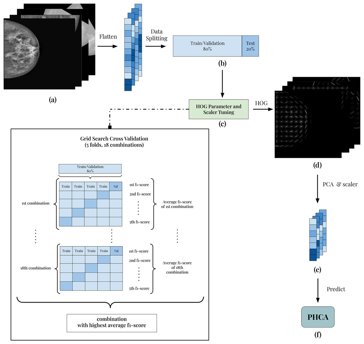
Figure 1: Illustration of the framework of the breast cancer classification scheme.
(A) Each image is grayscaled. (B) HOG is implemented to obtain its corresponding descriptors with 54,756 dimension. (C) The dataset is then prepared by first dividing into training and testing with 80:20 ratio. After which, the data are normalized using Standard Scaler. (D) Then, PCA is performed to reduce the dimensions of the features. (E) Reduced features are scaled using best scaler obtained in the tuning stage. (F) Finally, the scaled features are used to predict benign and malignant mammography scans using PHCA.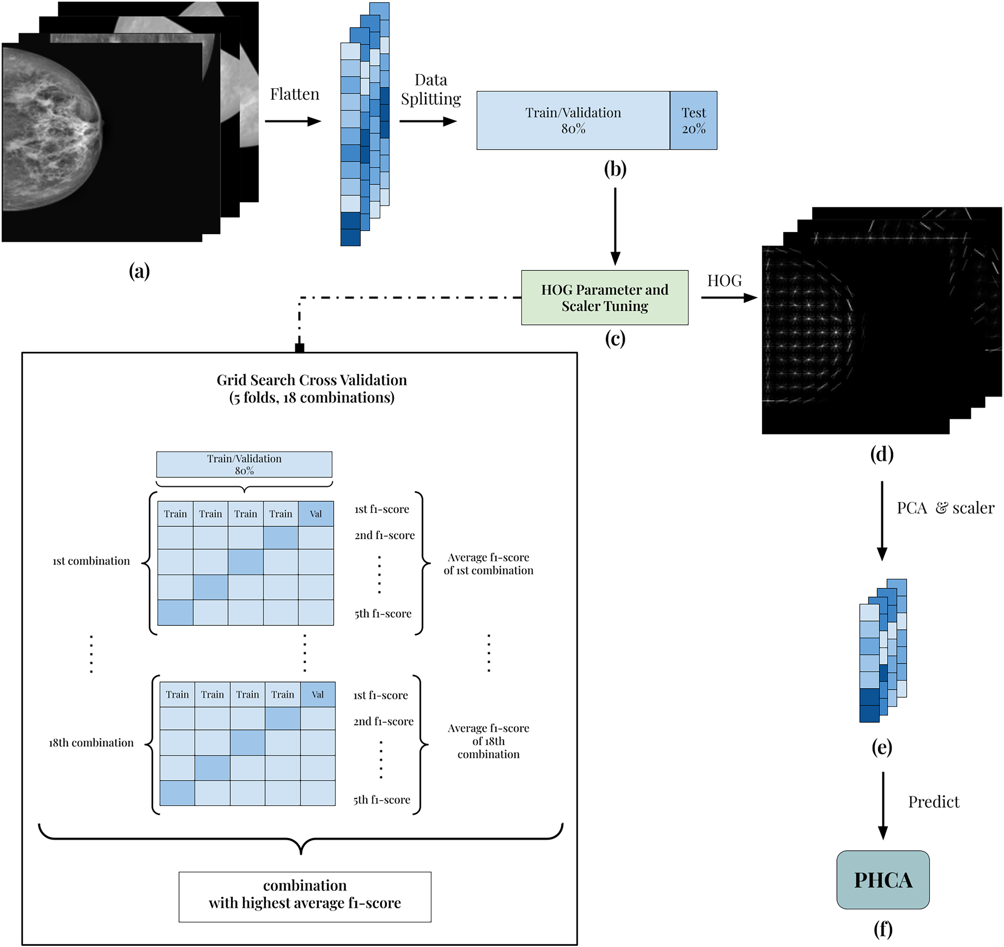
| HOG parameters | Scalers | |
|---|---|---|
| Pixels per cell | Cells per block | |
| 4 4, 8 8, 16 16 | 2 2, 3 3 | Standard, Minmax, Robust |
As an example, the first combination of parameters and scaler is 4 × 4 pixels per cell (PPC), 2 × 2 cells per block (CPB), and Standard scaler. Using 5-fold cross-validation, the training and validation folds undergoes feature extraction using HOG with 4 × 4 PPC, 2 × 2 CPB, and nine orientations. Then, the extracted HOG descriptors is reduced using PCA with a standard 95% parameter. Finally, the reduced features are scaled using Standard scaler and the output of which is used to train the PHCA model. For each fold, the F1-score is calculated and the average F1-score across the five folds is obtained. This serves as the “score” of the HOG parameter and scaler combination in the tuning process.
The parameter and scaler combination having the best average F1-score is then used to predict the 20% training set. The corresponding HOG parameters of this combination are used to extract the HOG descriptors (Fig. 1D). Then, using PCA with 95% parameter and the corresponding scaler in the best combination, the final features are obtained (Fig. 1E). Finally, classification is implemented using PHCA on these features (Fig. 1F). The output of PHCA is a vector of binary values (0 or 1) representing the predicted class of each test data. The performance of PHCA is then quantified using five evaluation metrics: precision, recall, F1-score, specificity, and overall accuracy.
The specified combinations in Table 3 are declared based on studies that used HOG for similar application. The PCA is used with a standard 95% parameter to preserve at least 95% of total variance of the dataset. This is set based on common practice on use of the algorithm. In this way, dimension reduction capability of PCA is maximized while minimizing the information loss. Similar strategy is set for the orientations parameter of HOG, using a standard of nine in the experiment.
The implementation in this article is done on a computer with the following configurations: 3,401 MHz AMD Ryzen 9 5950X 16-core processor, NVIDIA GeForce RTX 3080 graphics cards, 64 GB 3,200 MHz RAM, and a 1 TB solid-state drive. For reproducibility, the repository code is available at https://doi.org/10.5281/zenodo.14862036 (Jetomo, 2025).
Results and discussion
HOG parameter and scaler tuning
The 80% training/validation set is used to identify the best combination of HOG parameters (PPC and CPB) and scaler in terms of average F1-score. Table 4 shows the implementation result on this tuning stage. The table shows that the average F1-score ranges from 90.58% to 95.74% which indicates good overall performance of the data preprocessing algorithms used. On average, the combinations having PPC with variations in CPB and scaler resulted in the least average F1-scores (90.82%). Meanwhile, the combinations with and PPC obtained at least 95% average F1-scores, considering the margin of errors. For CPB, the parameter obtained a better overall average F1-score of 93.94% than having 93.64%. Additionally, the standard, minmax, and robust scalers obtained an average F1-score of 93.75%, 93.93%, and 93.70%, respectively, indicating no significant differences in their contribution to the result.
| Pixels per cell | Cells per block | Scaler | |
|---|---|---|---|
| 2 × 2 | 3 × 3 | ||
| 4 4 | 95.39 0.63 | 95.74 0.49 | Standard |
| 95.32 0.64 | 95.40 0.72 | Minmax | |
| 95.32 0.71 | 95.20 0.63 | Robust | |
| 8 8 | 90.58 0.87 | 90.69 0.93 | Standard |
| 91.09 1.08 | 91.10 1.18 | Minmax | |
| 90.68 0.96 | 90.75 0.88 | Robust | |
| 16 16 | 94.71 0.93 | 95.40 0.82 | Standard |
| 94.94 0.82 | 95.74 0.71 | Minmax | |
| 94.79 0.79 | 95.40 0.82 | Robust | |
Comparing all combinations altogether, both , , standard and , , minmax combinations obtained the highest average F1-score of 95.74%, with the former being more robust due to its smaller margin of error. Due to this result, we use both combinations in classifying the test set and compare their performance in terms of the various classification metrics and computational efficiency.
Classifying the test set
In the final classification stage, the PHCA model is trained using the 80% or 6,105 training images used for tuning the HOG and scaler. Then, the 20% or 1,527 test images were predicted using the trained PHCA model. In the test set, 504 images are benign while 1,023 images are malignant, capturing the distribution of the classes in the entire dataset. The results of this classification is shown in Table 5. The table highlights the final classification result of the two best HOG parameter and scaler combinations in the tuning stage: combination A represents the PPC and standard scaler and combination B represents the PPC and minmax scaler, both of which has CPB.
| Combination | Pre | Rec | F1 | Spec | Acc | ||||
|---|---|---|---|---|---|---|---|---|---|
| 0 | 1 | 0 | 1 | 0 | 1 | 0 | 1 | ||
| A | 97.03 | 95.64 | 90.87 | 98.63 | 93.85 | 97.11 | 95.64 | 97.03 | 96.07 |
| B | 95.48 | 98.23 | 96.43 | 97.75 | 95.95 | 97.99 | 98.23 | 95.48 | 97.31 |
For combination A, the number of HOG descriptors obtained are 236,196. Reducing this using PCA, the final feature vector size is 2,432. On the other hand for combination B, the HOG descriptors has dimension 11,664 while the final feature vector size is 739, significantly smaller than the first (see Table 6). Table 5 shows that the classification scores of the two combinations are consistently high, both for class 0 (benign) and class 1 (malignant) images.
| Dimensions | Combination | |
|---|---|---|
| A | B | |
| No. of HOG descriptors | 236,196 | 11,664 |
| Final feature vector size | 2,432 | 739 |
| Computation time | ||
|---|---|---|
| Segment | A | B |
| Data preparation | 1,078.0335 | 128.5180 |
| Training | 3.3858 | 3.4128 |
| Predicting | 4,837.6744 | 4,623.5121 |
| Total | 5,919.0937 | 4,755.4429 |
Initial analysis on the scores shows that combination A and B have variations in performance per metric. For precision, combination A obtained a higher value for class 0 (97.03%) than class 1 (95.64%) whereas combination B obtained higher for class 1 (98.23%) than class 0 (95.48%). Recall scores reflect a different observation. Here, both combinations A and B obtained higher values for class 1. However, the difference in recall score of combination A for benign and malignant images is whereas the same quantity for combination B is . This indicates robustness of combination B’s precision against data imbalance as noted that there are twice as much malignant than benign test images. The same observation is true for F1-score. Combination A still resulted with a higher difference in F1-scores for class 0 and 1 than combination B. This additionally indicates that robustness is more observed in combination B in terms of F1-score, a metric that incorporates both precision and recall.
Specificity tells a different story. For combination A, a higher specificity score is obtained for class 1 while combination B scored higher for class 0. However, in class 0, combination B still obtained higher specificity scores than combination A. The overall accuracy value further highlights how combination B outperforms combination A by scoring 97.31%, 1.24% better than the other. From these analyses, we’ll dig further our discussion on the result of combination B. The confusion matrix of which is provided in Fig. 2.
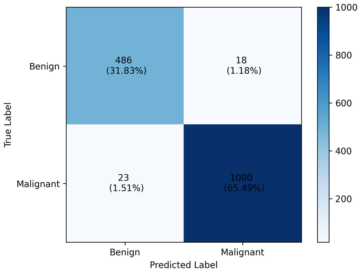
Figure 2: Classification report of the PHCA model.
The result shows that obtained precision, recall, F1-score, specificity per class and the overall accuracy of the PHCA model.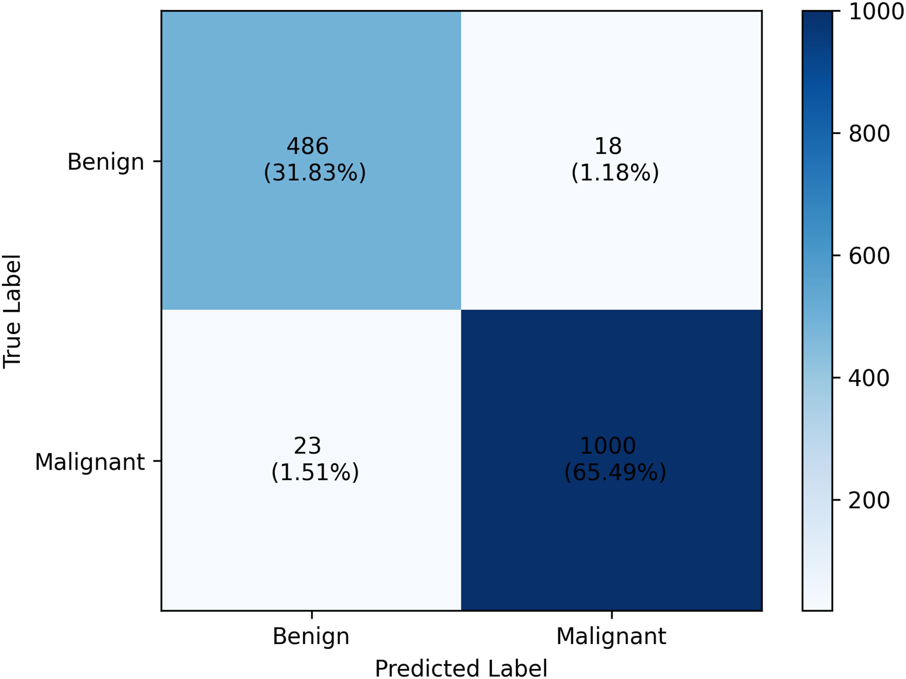
Deep dive on combination B results
The precision score obtained by PHCA for class 0 and class 1 are and , respectively. This means that approx. 95% of the images classified as benign were correctly identified as such, while approx. 98% of the images classified as malignant were correctly identified. High precision values for both classes imply that the model makes very few misclassifications of benign images as malignant images, or vice versa, which is crucial for minimizing unnecessary treatments or misdiagnosis. Furthermore, using combination B, the recall values of the two classes were 96.43% for benign and 97.75% for malignant cases. This means that 96.43% of benign and 97.75% of malignant tumors in the test group were correctly classified by the model. The slight discrepancy between the recall values for benign and malignant tumors could be a result of the great imbalance between the number of benign and malignant images in the test set.
The high precision and recall values of PHCA with combination B, especially for the malignant case, highlights the strong potential of the model as a medical decision-support tool. In practice, the high recall value for malignant tumors is important as it indicates that the model is very sensitive to the presence of malignancy and ensures that very few malignant cases go undetected. Also, the high precision value shows that the model makes highly trustworthy predictions since the malignancy diagnosis is said to be correct 98% of the time. Together, the model ensures that malignant tumors are detected while limiting false positive on the benign tumors. At the same time, the model guarantees that malignant tumor diagnosis are trustworthy, suggesting its effectiveness in detecting malignant tumors from the mammography scans. This could be of great benefit in a real-life medical screening context where false negative results (missed malignant tumors) are highly undesirable.
The F1-scores, 95.95% for benign and 97.99% for malignant, also confirm the strong performance of the model. These values show that the model strikes an excellent balance between precision and recall and provides comprehensive measure of its ability to correctly classify both tumor types. The higher F1-score for malignant cases shows that the model is particularly good at discriminating malignancies—a crucial ability to reduce the risk of misclassifications in a diagnostic setting.
Specificity, another important metric, measures the model’s ability to correctly identify images that do not belong to a particular class. Specificity scores of 98.23% for benign and 95.48% for malignant indicate that the model is good at classifying images that do not belong to a particular class. High specificity means that the model effectively avoid false positives, important in medical diagnosis to avoid unnecessary stress for patients or the need for further invasive tests or interventions when there is no malignancy. The highly balanced values for recall and specificity indicate also that the model is robust and well-calibrated, minimizing the risk of both false negative and false positive results.
The overall accuracy of the model was 97.31%, reflecting the proportion of correct predictions out of the total number of classifications made. This accuracy is significant and demonstrates that the proposed method, which combines persistent homology with PCA and HOG, provides a reliable framework for classifying mammography scans. An accuracy of at least 97% on a task as sensitive and complex as breast cancer diagnosis emphasizes the robustness of the model and its potential for real-world application in early detection systems.
Computational complexity analysis
The computational times of the PHCA model together with two HOG parameters and scaler combinations are monitored and summarized in Table 6. The corresponding feature dimensions for each stage of the data preprocessing are also provided. From the result, it is clear that the choice of data preprocessing technique, either of the two combinations, had a major impact on the overall computational cost.
Combination A required 1,078.03 s or approx. 18 min to extract the features while combination B did the same task in only 128.52 s or approx. 2.14 min. From these values, it shows that data preparation takes at least 8 times longer for combination A than B. This reflects the added computational complexity of a more granular PPC parameter of the HOG algorithm— for combination A compared to for B. Using smaller cell size implies that gradient orientations are computed at a finer spatial resolution, producing a larger number of descriptors—almost 240,000 for combination A while only 12,000 for combination B.
On the other hand, the training time of both combinations required only s or 0.05 min. This indicates that the preprocessing approach, at least between combinations A and B, does not significantly affect model training complexity even with the significant difference in size of the final feature vectors of the two combinations. This suggests that the information to distinguish between benign and malignant scans captured by the 2,432-dimensional feature vectors of combination A is also captured by the more memory-efficient 739-dimensional feature vectors of B.
Meanwhile, the predicting time of combination A took 4,837.67 s or 80.63 min to predict 1,527 test images while combination B took 4,623.51 s or 77.06 min for the same task, slightly faster than that of combination A. The s difference is also largely due to the size difference of the final feature vector of the two combinations. The PHCA model required fewer computations for a smaller-sized feature vector from combination B, resulting with a smaller prediction time per image. This suggests that the lighter data preprocessing of combination B may lead to marginally more efficient inference.
From the previous section, we highlighted how combination B outperformed combination A in terms of overall classification performance. Despite the more detailed representation of the images using combination A with the PPC, the added preprocessing time does not justify its results being similar or worse in some cases to that of combination B. For practical applications, a breast cancer diagnostic tool requires efficiency and trustworthy results. The faster overall classification runtime of combination B and its demonstrated robustness and strong performance with the PHCA model further justifies its reliability for the task.
Comparison with existing literature
In Table 7, we present the performance comparison of our proposed method with existing literature that used the same INbreast dataset. Papers cited here have implemented varying preparation techniques while some used the same 7,632 images as in this article. Majority of the existing literature utilized deep networks, specifically CNN-inspired models, to distinguish benign from malignant mammography scans.
| Reviewed works | Model | Results | ||||
|---|---|---|---|---|---|---|
| Pre | Rec | F1 | Spec | Acc | ||
| Proposed | PHCA | 96.86 | 97.09 | 96.97 | 96.86 | 97.31 |
| El Houby & Yassin (2021) | CNN | – | 96.55 | – | 96.49 | 96.52 |
| Karthiga, Narasimhan & Amirtharajan (2022) | CNN (RMS Prop) | – | – | – | – | 96.53 |
| Jabeen et al. (2023) | MGSVM | 99.60 | 99.55 | 99.57 | – | 99.60 |
| Cubic SVM | 99.40 | 99.40 | 99.40 | – | 99.40 | |
| Yadav & Kumar (2025) | Frac-CNN | – | 99.00 | – | 98.20 | 99.35 |
| ResNet50 | – | 98.30 | – | 97.00 | 96.86 | |
| DenseNet | – | 96.80 | – | 96.30 | 97.60 | |
| CNN-SVM | – | 95.80 | – | 95.20 | 96.50 | |
El Houby & Yassin (2021) used 387 out of the 410 raw images where the INbreast dataset originated. Noise removal, image enhancement using CLAHE, and region of interest (ROI) extraction has been used to obtain the features from the images. A fine-tuned CNN model was trained which resulted with a recall, specificity, and accuracy of 96.55%, 96.49%, and 96.52%, respectively. A similar approach is proposed by Karthiga, Narasimhan & Amirtharajan (2022) but using Polynomial Curve Fitting as their segmentation technique to partition the input image into multiple regions that are easy to isolate and analyze, and thus construct the ROI. Classifying their extracted features using CNN with RMS Prop optimizer, the authors were able to obtain an accuracy of 96.53%. The proposed work offers improvements to these results as reflected in the obtained metrics shown in Table 5. Additionally, the proposed work did not require any noise removal, ROI extraction, or a deep network like CNN to achieve a better result, highlighting the capability of the HOG descriptors and PH-based model for the task.
More recent literature offers a more complex approach to the problem. Jabeen et al. (2023) proposes a hybrid framework to extract features from the INbreast images. The authors used their haze-reduced local-global method for contrast enhancement, extracted deep features using a pre-trained EfficientNet-b0 model, and applied feature selection technique using their Equilibrium-Jaya controlled Regula Falsi. A feature fusion strategy is applied by the authors which resulted with an accuracy of 99.60% using the Medium Gaussian SVM (MGSVM) model. With the feature selection strategy, they obtained a slightly lower accuracy (99.40%) using Cubic SVM but with a significant reduction in computation time (2.20 s from 20.01 s of MGSVM). These results clearly outperformed PHCA but the marginal performance gap of 3–4% can be clinically accepted. Also, Jabeen et al. (2023) uses a 50:50 train-test ratio with a more balanced set of images (1,216 benign and 1,120 malignant) whereas our proposed work still performed strongly on a 80:20 train-test ratio with a significantly imbalanced dataset (2,520 benign and 5,112 malignant). The proposed feature selection strategy, however, clearly outperforms the proposed work since the PHCA model predicts an image for about 3.03 s whereas that of Jabeen et al. (2023) takes 0.018 s, indicating an area of improvement for PHCA.
In Yadav & Kumar (2025), the authors proposes an advanced image-filtering method through adaptive mean filtering which enhances the quality of the mammography scans. They used the Particle Swarm Optimization algorithm to optimize a Fractional CNN (Frac-CNN) and compared this with state-of-the-art models like ResNet50, DenseNet, and CNN-SVM using the same data preparation framework. With a 70:30 train-test on the INbreast dataset identical to this article, the authors achieved 99.00% recall, 98.20% specificity, and 99.35% accuracy using the fine-tuned Frac-CNN model, outperforming the state-of-the-art models and the proposed work. The authors highlighted that the training time of Frac-CNN is 7 h on 7,632 images (or approx. 3.30 s per image), about 5–10% increase compared to standard CNNs. Comparing this with the training time of our proposed work which is 3.41 s on 6,105 images (or approx. 0.0006 s per image), indicating less complexity of the PHCA model in terms of training capability. Moreover, from the result of Yadav & Kumar (2025) on the state-of-the-art models, we can also see how the proposed work performed at par, if not better, in some of the metrics. PHCA is shown to outperform DenseNet and CNN-SVM in recall and specificity which are priority metrics for breast cancer diagnosis. The model also exceeded ResNet50 in terms of accuracy, a good indicator for a model’s classification power. This further highlights how PHCA can offer strong results with fewer parameter configurations and less complexity than deep networks.
Conclusions
The proposed work introduces the use of PHCA to overcome the challenges in breast tumor misdiagnosis and delayed treatment. PH, a core technique in topological data analysis, was used to capture topological features from complex medical data. The advantage of PH lies in its ability to extract significant topological structures such as connected components, loops, and gaps, enabling medical images to be analyzed at multiple levels. This capability allows PH to distinguish between benign and malignant tumors with greater precision and provides a powerful solution to the limitations of conventional imaging techniques.
Several preprocessing steps were implemented, including the use of HOG for feature extraction and PCA for dimensionality reduction. With a fine-tuned HOG algorithm and scaler, the PHCA model achieved an impressive 97.31% accuracy. In addition, the precision and recall values of 96.86% and 97.09% were respectively obtained, demonstrating the effectiveness of the model in minimizing false positives and false negatives. The F1-score and specificity also confirmed the consistent performance of the model in both classes, indicating its robustness and reliability.
The proposed method shows significant potential for improving breast cancer screening programs. While it is not the best in the literature, it offers at par, sometimes better, performance than more computationally expensive state-of-the-art models even for highly imbalanced datasets. By identifying topological features that reflect crucial information about tumor structure, a more accurate differentiation between benign and malignant tumors can be achieved. In addition, the scalability of PH enables its application to larger data sets and more complex imaging tasks beyond breast cancer diagnosis, e.g., ultrasound, magnetic resonance imaging (MRI), or digital breast tomosynthesis (DBT). Integration of PH into existing computer-aided diagnosis systems could lead to significant improvements in early detection and diagnosis, ultimately contributing to better patient outcomes.
Limitations and future directions
It is noted that the proposed work is constrained in terms of the preprocessing algorithms used, limited comparison with state-of-the art models, and application to only one dataset. The following future steps could be done to address these limitations.
Further refinements of the approach can be done by exploring other parameters for the preprocessing techniques. A more exhaustive search algorithm can be implemented, e.g., random search cross validation, Bayesian optimization, or metaheuristic approaches like particle swarm optimization and Genetic Algorithm to identify best parameters. Other preprocessing algorithms can also be explored to identify which works best with the topology-based classifier.
While PHCA is compared with existing literature, benchmarking PHCA with baseline methods (e.g., SVM, ensemble-based models, neural networks, etc.) using the same preprocessing approach can be implemented to have a one-to-one comparison. This comparison may focus on classification performance, computation time, and resources consumption.
Use PHCA and the proposed approach to other datasets such as the CBIS-DDSM (Sawyer-Lee et al., 2016) and MIAS (Suckling et al., 2015) database. This can offer a more comprehensive performance evaluation and help identify which breast cancer data structures is more applicable for the model.
The authors also aim to coordinate with radiologists or medical institutions to deploy and evaluate the proposed approach in a clinical setting. This will provide additional insights on the model’s performance in real-world diagnostic systems.