
Assessing the risk of falling in community-dwelling older adults through cognitive domains and machine learning techniques
- Published
- Accepted
- Received
- Academic Editor
- Davide Chicco
- Subject Areas
- Algorithms and Analysis of Algorithms, Artificial Intelligence, Computer Vision, Data Mining and Machine Learning, Social Computing
- Keywords
- Artificial intelligence, Cognition, Cognitive function tests, Pattern recognition, Postural balance
- Copyright
- © 2025 Prieto et al.
- Licence
- This is an open access article distributed under the terms of the Creative Commons Attribution License, which permits unrestricted use, distribution, reproduction and adaptation in any medium and for any purpose provided that it is properly attributed. For attribution, the original author(s), title, publication source (PeerJ Computer Science) and either DOI or URL of the article must be cited.
- Cite this article
- 2025. Assessing the risk of falling in community-dwelling older adults through cognitive domains and machine learning techniques. PeerJ Computer Science 11:e3367 https://doi.org/10.7717/peerj-cs.3367
Abstract
Background
Older people’s falls are a global public health problem, leading to injuries, disability, and fatalities. Using screening tools to measure predictive factors is essential for assessing the risk of falls among older adults. The literature highlights executive function tests as a way to assess this risk. They are also economical and reliable tools. Therefore, a Machine Learning (ML) technique based on variables obtained from cognitive domains could classify an older adult as at high or low risk of falling.
Methodology
The study collected six variables from 50 community-dwelling older adults. The variables included age, educational level, and Trail Making Test (TMT) part B, Digital Span Backward, Stroop Color-Word Interference, and Mini Balance Evaluation Systems Test (Mini-BESTest) tests. These variables fed three ML models to predict if an older adult is at high or low risk of falling. Specifically, we considered Logistic Regression (LR), Decision Trees, and K-Nearest Neighbors. The proposed models were assessed using a bootstrapping sampling method and an aggregated confusion matrix, from which typical performance metrics were derived. The input variables in the best model were selected using a wrapper-based selection method.
Results
Of the three models, the LR classifiers were top-ranked based on accuracy, with a maximum value of 71.4%. The best classifiers included the educational level or the TMT part B as input variables. Thus, these variables were strong predictors of fall events in the population study. We tested the input variables to ensure they were significant for the best LR classifiers and assessed model performance, generalization, and stability given the dataset sample size.
Discussion
We weighed the performance metric results with a clinical perspective to select the best LR classifier. Thus, the more suitable model resulted in the classifier with TMT part B and educational level as input variables. Besides presenting competitive performance results, it enables us to consider a broader range of clinical information and draw more informed conclusions. Comparing our proposed model with four assessment tools, we observe it was second in Area Under the Receiver Operating Characteristic Curve (AUC) and third in accuracy.
Conclusions
In this work, we developed an LR classifier to identify older adults with high or low risk of falling, using the TMT Part B test and the educational level as features. In addition, we provided cut-off values to assess the risk of falling using only the TMT part B test or the educational level. We found that, individually, 8 years or more of schooling or a result of the TMT part B lower than 212 s are associated, on average, with a low risk of falls. The Chilean health system can broadly implement the best classifier since the input variables are easy to collect, and the classification rule can be calculated using simple arithmetic operations.
Introduction
Older people’s falls are a global public health problem (Arkkukangas et al., 2019). Approximately 30% of adults over the age of 65 experience a fall annually, and the occurrence increases with age (Montero-Odasso et al., 2022). Moreover, falls are the primary cause of injuries, disability, and fatalities within this population (Smith et al., 2014; Vieira, Palmer & Chaves, 2016). In particular, falls accounted for roughly 80% of the disabilities resulting from unintentional injuries (Smith et al., 2021).
Falls result from a mix of intrinsic, extrinsic, and behavioral factors (Jain, Schweighofer & Finley, 2024; Patel & Hoque, 2025). Some examples of intrinsic factors include mobility issues, a history of falls, cognitive problems, and balance difficulties (Sturnieks et al., 2025). In this sense, balance allows individuals to position their center of mass within their base of support and, in this way, achieve the necessary functionality to perform the tasks associated with the different stages of life.
This work aimed to identify when an community-dwelling older adult is at high or low risk of falling through a Machine Learning (ML) classifier based on the assessment of five input variables, which were obtained from a previous study (Martínez-Carrasco et al., 2025). The variables were age, educational level, and three executive function tests. As a measure of the risk of falling, we employed the results of the Mini Balance Evaluation Systems Test (Mini-BESTest), which we binarize to get a 0/1 variable, representing a high or low risk of falling.
Cognitive functions play a critical role in falls in older people (Guo et al., 2023; Smith et al., 2023). In particular, the educational level is among the cognitive protective factors for preventing falls in older adults. Having less than 6 years of schooling significantly increases the risk of future falls in community-dwelling older adults (Lee et al., 2021).
In relation to cognitive domains, executive function has a significant impact on postural balance (Martínez-Carrasco et al., 2025; Davis et al., 2017; Mirelman et al., 2012). A good executive function can compensate for age-related changes that increase the risk of falling (Muir-Hunter et al., 2014). Thus, this relationship can be used to determine fall risk in older adults through several widely known executive function tests.
Currently, several tests and screening tools are used to assess the risk of falls in community-dwelling older adults (Colón-Emeric et al., 2024; González-Castro et al., 2024; Montero-Odasso et al., 2022; Ong et al., 2023). These tools usually focus on assessing motor aspects related to falling, such as the Timed Up and Go (TUG) (Barry et al., 2014), Berg Balance Scale (Berg et al., 1992), Tinetti (Tinetti, Williams & Mayewski, 1996), and Unipodal Stance test (Mancilla, Valenzuela & Escobar, 2015). Even though we understand that these tests are commonly used to assess the risk of falling, there may be some contexts in which they are more complex to use, either because they require more time or space to be administered (Eichler et al., 2022; Fong et al., 2023; Khatib et al., 2025). Furthermore, some questionnaires or screening tools such as Activities-Specific Balance Confidence Scale (ABC-16) (Powell & Myers, 1995), Short FES-I (Kempen et al., 2007) or STEADI (Stevens & Phelan, 2013) may have “social desirability bias”, i.e., people may give answers to make themselves appear healthier than they really are (Lensvelt-Mulders & Boeije, 2007), and also some tests cannot be used in isolation as a screening tool to predict falls (Lima et al., 2018; Montero-Odasso et al., 2021).
Considering the above, executive function assessment tests are a good alternative to estimate the risk of falls (Mirelman et al., 2012; Newkirk et al., 2022; Smith et al., 2023). Executive function tests have the advantage of being generally performed with paper and pencil, requiring no major infrastructure or large physical space for their application. As they are low-cost tools, they can be used by various health professionals for screening purposes. For example, using an ML technique, Mateen et al. (2018) determined that the Trail Making Test (TMT) was a good predictor of falls during the in-patient stay.
The main contributions of this work are:
We developed an ML-based classifier that functions as a screening tool to identify when a community-dwelling older adult is at high or low risk of falling based on the educational level and the TMT part B results. The classifier employs the Logistic Regression (LR) model and achieves an accuracy of 69.7%.
We found that, when considering TMT part B (Mandonnet et al., 2020), Digital Span Backward (DSB) (Rosas, Tenorio & Pizarro, 2012), and Stroop Color-Word Interference (SCWI) (Scarpina & Tagini, 2017) executive function tests to assess the risk of falls, TMT results include information of the other variables. Adding the other executive function tests to the ML model did not improve accuracy. This result was consistent with our previous work (Martínez-Carrasco et al., 2025).
Besides the best model, we obtained two additional models that only consider the educational level or the TMT part B result as input. These models allow for determining cut-off values that separate individuals by their risk of falling. Considering these factors separately, on average, 8 years or more of schooling or a result of the TMT part B lower than 212 s are associated with a low risk of falls.
The rest of this work is organized as follows: in ‘Related Work’, we review related work. Then, in ‘Materials and Methods’, we present the study design and the methodology used to develop the ML classifier. In ‘Results’, we show the results obtained from the study. Next, in ‘Discussion’, we discuss our results, highlighting the main findings and their practical implementations. Finally, the conclusions of this work are presented in ‘Conclusions’.
Related work
ML techniques have been previously used for fall risk assessment with different objectives, such as predicting a person’s fall within a specific time frame (Allcock et al., 2009; Deschamps et al., 2016; Lockhart et al., 2021; Makino et al., 2021; Mishra et al., 2022; Oshiro et al., 2019; Ye et al., 2020), identifying patients with high fall risk (Ikeda et al., 2022; Mateen et al., 2018; Panyakaew, Pornputtapong & Bhidayasiri, 2021; Shumway-Cook, Brauer & Woollacott, 2000; Sun, Hsieh & Sosnoff, 2019; Zhou et al., 2024), and detecting a person’s fall (Al-qaness et al., 2024; Liu, Sun & Ge, 2025; Lupión et al., 2025). The techniques most frequently used are K-Nearest Neighbors (K-NN) (Mishra et al., 2022), Decision Trees (DT) (Deschamps et al., 2016; Makino et al., 2021; Mishra et al., 2022), eXtreme Gradient Boosting (XGBoost) (Ikeda et al., 2022; Panyakaew, Pornputtapong & Bhidayasiri, 2021; Ye et al., 2020), Random Forest (RF) (Ikeda et al., 2022; Lockhart et al., 2021; Mateen et al., 2018; Mishra et al., 2022; Sun, Hsieh & Sosnoff, 2019; Zhou et al., 2024), Convolutional Network (CN) (Al-qaness et al., 2024; Liu, Sun & Ge, 2025; Lupión et al., 2025), and LR (Mishra et al., 2022; Oshiro et al., 2019; Shumway-Cook, Brauer & Woollacott, 2000; Zhou et al., 2024).
Deschamps et al. (2016) devised an ML model to predict if an older adult will fall for the first time during the next year. At the beginning of this study, 73 input variables taken from medical, demographical and physical data, were obtained from adults that had never fallen. Falls were then recorded during the following year. The resulting DT classifier showed an accuracy of 89%.
Ye et al.’s (2020) work seeks to forecast patients’ fall risk. To that end, Electronic Health Records (EHR) from patients of more than 65 years of age were fed into a model. The resulting algorithm identifies patients with low, medium, or high risk of falls during the next year. Additionally, the model discovered that abnormalities of gait and balance, and fall history are among the strongest predictors of future fall events.
Song et al. (2024) examined fall risk screening in primary care. They compared traditional questionnaires with machine learning models trained on longitudinal EHR data records from primary care practices of community-dwelling older adults. The questionnaire-based method reached an Area Under the Curve (AUC) of 0.59, while the best ML models achieved up to 0.76. Key predictors identified included age, history of fall injuries, and issues related to gait or mobility.
A fall risk assessment tool for inpatients based on 6 years of hospital records is presented in the work of Jahangiri et al. (2024). Thirteen variables were considered in this method, which were divided into extrinsic (such as medication, hospital department, and work shift) and intrinsic (such as age and mobility) factors. They tested four machine learning algorithms. With an accuracy of 0.74 and an AUC of 0.72, the deep neural network demonstrated the best predictive performance. The authors additionally showed that distinct models for morning, afternoon, and night shifts improved the prediction of fall risk, taking into account variations in hospital schedules and care conditions.
In the work described in Oshiro et al. (2019), 10 years of EHR data were used to predict a fall within the following year. Individuals required 2 years with no record of falling to participate in the study. Although the risk of falling is multi-factorial, this study reported that comorbidities, walking issues, and poly-pharmacy were among the main factors.
Likewise, Mishra et al. (2022) proposed an ML-based model to predict a fall within the next 6 months, using geriatric assessments, gait variables, and fall history. Similarly, Makino et al. (2021) trained a DT classifier to predict falls within the next year by including the TUG test in the baseline survey, in addition to data from demographics, gait variables, medications, and fall history.
Mateen et al. (2018) studied if falls during the in-patient stay could be predicted using cognitive and motor function tests, and demographics. The TMT part B was the only test used to measure executive function, resulting in the best predictor of falls, and, surprisingly, adding other variables to the model did not improve predictions. This result suggests that TMT part B data collection alone may be sufficient for predicting falls. In our work, we combined three executive function tests, which include TMT, as inputs to the ML model. As a significant result, we obtained that, out of the three tests, only TMT part B remained as an input variable of the optimal classifier after a wrapper-based feature selection. In contrast to Mateen et al. (2018) in our case the population consisted of community-dwelling older adults. In addition, Mateen et al. (2018) used different ML methods, one of them being RF, which cannot provide simple cut-off scores for different fall risk categories. In our work, the top-ranked classifiers used LR models. We found cut-off values for TMT part B and educational level variables to predict the risk of falls. Besides, the LR model allows assessing the impact of the input variables improvement in the odds of the patient presenting a low risk of falling.
The TUG functional mobility test was studied by Shumway-Cook, Brauer & Woollacott (2000) as a way to identify individuals prone to falls. The authors assessed 15 older adults with a history of two or more falls in the previous 6 months and 15 with no history of falls. An LR model determined a TUG cut-off value of 14 s to classify an older adult in faller/non-faller, with 90% of accuracy. Similarly, Roshdibenam et al. (2021) used the TUG test plus non-intrusive wearable sensors to measure the gait kinematics of the participants. This study evaluated 100 older adults aged 65 years or older, and they determined a TUG cut-off value of 14 s to classify an older adult in faller/non-faller, with an accuracy of 71%. In our work, we determine cut-off values for the educational level and the TMT part B that separate older adults at high/low risk of falls, with accuracies of 71.4% and 64.7%, respectively. The normative values of TMT use an age distribution to assess the risk of falling in percentiles (Groth-Marnat, 2003). In our study, a sample of persons aged 61 to 86 was considered, so the cut-off score determined corresponds to this age group.
Lockhart et al. (2021) proposed an RF classifier to detect older adults at risk of falls, within the next 6 months. The classifier was trained using gait features, including variability, complexity, and smoothness, collected from a wearable sensor during a 10-m walk test. The trained model achieved an overall 81% accuracy.
Panyakaew, Pornputtapong & Bhidayasiri (2021) proposed a classifier to differentiate Parkinson’s disease patients into fallers or recurrent fallers. Input variables included clinical demographics, medications, and the ABC-16. Their analysis revealed that specific activities, including sweeping the floor, reaching on tiptoes, and walking in a crowded mall, were significant predictors in the classifications. The identification of high-risk activities enables physicians to implement effective fall prevention strategies, thereby reducing the likelihood of future falls.
These studies show that ML techniques can predict fall risk in older adults across various scenarios. We observed that different types of predictors are frequently used, such as demographics, EHR, gait variables, fall history, and motor and cognitive tests. However, the influence of cognitive tests is not widely studied, despite TMT resulting in a strongly correlated predictor in the work of Mateen et al. (2018). For example, considering the review of González-Castro et al. (2024), none of the studies in that review based their ML models on data from cognitive tests, such as the TMT, DSB, or SCWI executive function tests.
The works by Ikeda et al. (2022) and Zhou et al. (2024) considered the educational level as a candidate predictor. The former used ML techniques such as RF to select predictors and XGBoost for modeling, while the latter used techniques such as LR, RF, and naive Bayes for modeling. However, the final model did not consider the educational level, as other variables were selected as better predictors of falling. This finding contrasts with the work of Lathouwers et al. (2022): they identified 24 risk factors for falls in older adults in the community, using ML techniques, where one of the most relevant factors was the educational level.
Materials and Methods
Participants and criteria for data collection
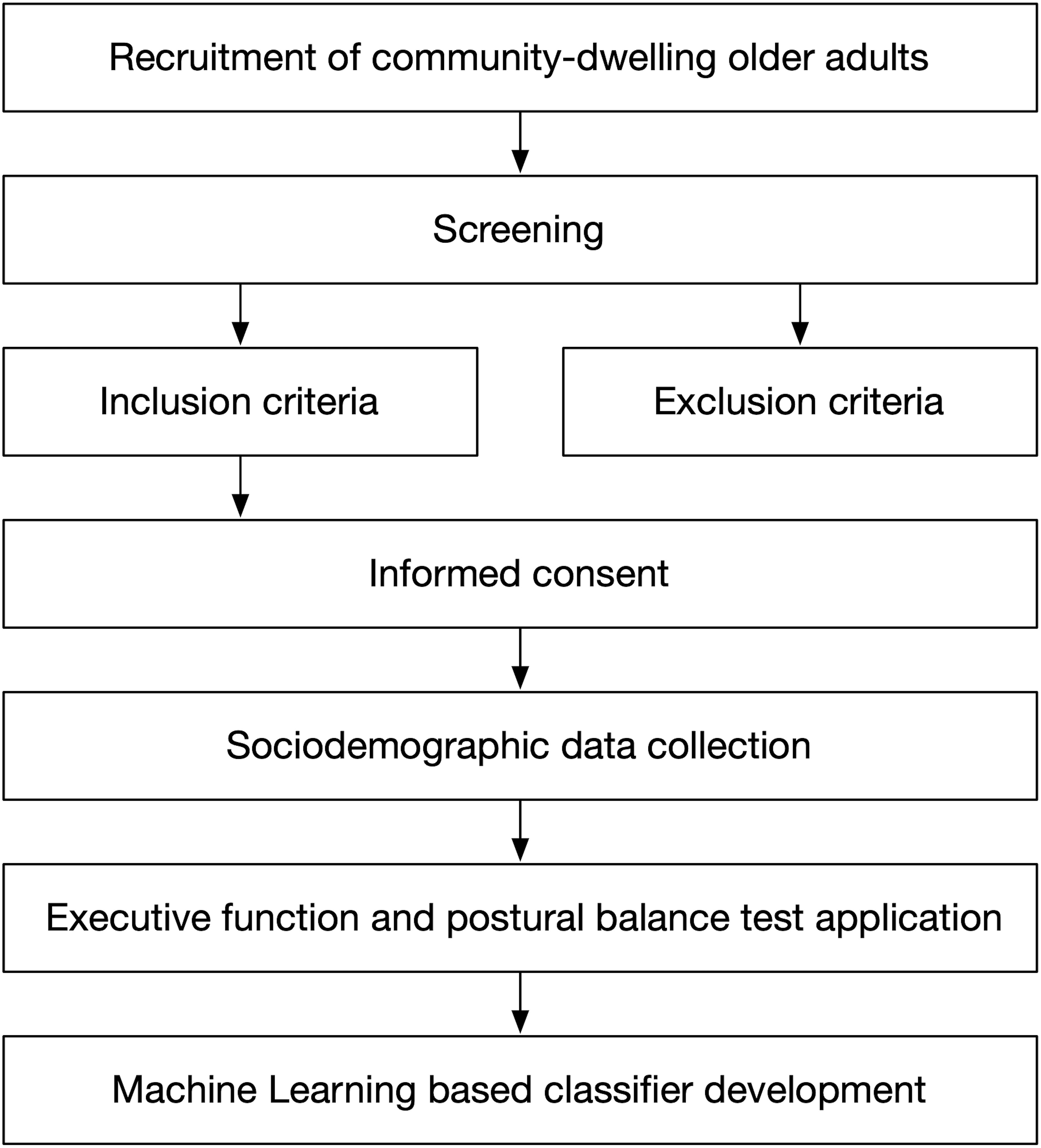
Figure 1 presents the seven stages carried out in this study. The first six stages are related to the participants’ description and data collection criteria. The last stage is related to the ML technique development.
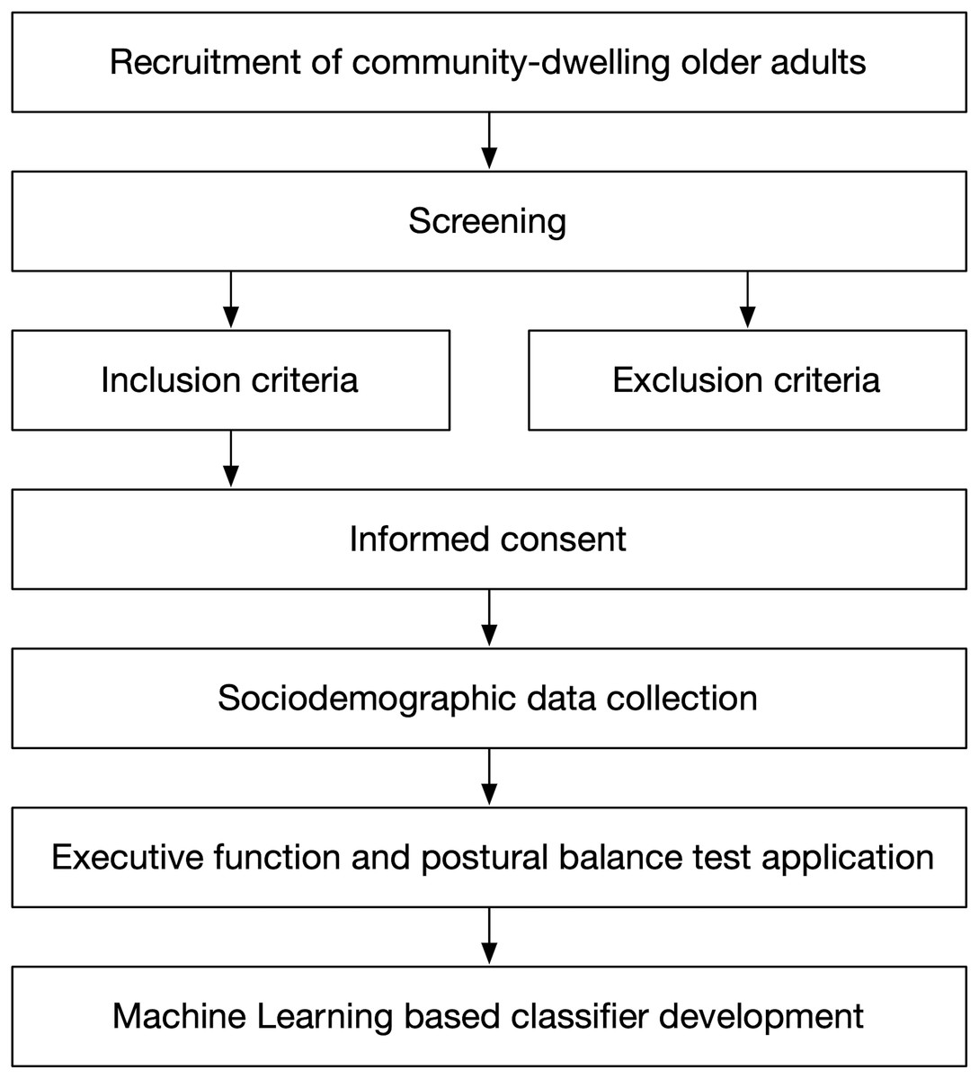
Figure 1: Study design overview.
The first stage at the top corresponds to population recruitment. They were older adults over 60 years of age who were participating in a community program aimed at promoting independence for older adults, as part of a Centro de Salud Familiar (CESFAM, in English, Family Health Center) initiative.
We conducted the second stage (screening), which consisted of determining who could participate in the study, by applying the inclusion and exclusion criteria (third stage), with those older adults who agreed to participate in the study.
The inclusion criteria were (1) age over 60 years, (2) with or without risk of loss of functionality according to the Chilean Evaluación Funcional del Adulto Mayor (EFAM, in English, Functional Assessment of Older Adults) (Thumala et al., 2017), (3) hemodynamically stable, and (4) ability to achieve independent gait (no human assistance) with or without technical aids. Meanwhile, the exclusion criteria were: (1) being illiterate or color-blind, (2) global cognitive impairment according to the Mini-Mental State Examination test (score 13 points), or (3) psychiatric pathology, vestibular disorders, Parkinson’s disease, Alzheimer’s disease, stroke, or severe sensory disturbances such as hearing or vision loss. The sample was non-probabilistic.
The study was approved by the Ethic Research Committee of the Talcahuano Health Service (Protocol No.: 77/2016), and complies with the ethical standards as laid down in the 1964 Declaration of Helsinki and its later amendments. Written informed consent was obtained from all participants at an informative meeting to explain the nature of the study (fourth stage).
We recorded the participants’ names, ages, previous relevant medical diagnoses, commonly used medications, and their fall history considering the number of falls during the previous year (fifth stage).
Two different test stations were established to administer the executive function and postural balance tests for each older adult. In the first station, the following tests were applied to assess executive function: the DSB test for evaluating updating, TMT part B for shifting, and the SCWI test for evaluating inhibition. In the second station, a physical therapist employed the Mini-BESTest (sixth stage) to assess the postural balance.
Methodology to obtain the optimal ML model
The development of the ML classifier (seventh stage) is composed of four steps:
Analyzing the study data, which is divided into two tasks. First, defining the binary fall-risk-level target variable to differentiate individuals with a high risk of falling from those with a low risk of falling. Next, discovering which features are more influential in predicting the risk of falling.
Validating classifier models for a small and imbalanced data set. In ML, models and data are hugely coupled due to the bias-variance tradeoff (Hastie, Tibshirani & Friedman, 2009; Kelleher, Mac Namee & D’arcy, 2020). Given a specific dataset, less complex models (linear, with a small number of parameters) may suffer from underfitting; meanwhile, more complex models (non-linear, with a large number of parameters) may end up presenting overfitting. In general, determining the optimal model for a dataset is carried out empirically. We proposed using classifiers with a low number of parameters, such as LR, DT, and K-NN, which we assessed using a bootstrapping sampling method and an aggregated confusion matrix (Kelleher, Mac Namee & D’arcy, 2020).
Selecting the optimal model based on: (i) the result of different performance metrics calculated from the aggregated confusion matrix, (ii) a clinical analysis of the best models.
Assessing dataset statistical implications on the optimal model performance, generalization, and stability. Datasets should be representative enough of the studies so that the trained models perform well and generalize outside datasets. Although there are a few rules of thumb to determine the minimal sample size (Rajput, Wang & Chen, 2023; Theodoridis & Koutroumbas, 2006), ensuring dataset sufficiency can be achieved by measuring model performance, generalization, and stability (Rajput, Wang & Chen, 2023). We conducted a numerical experiment to evaluate the impact of the sample size on model performance and generalization through a performance metric and the Cohen’s d estimator. Moreover, we evaluate model robustness and stability through the variation of the parameters as the sample size changes.
We performed experiments on a computer running Windows 11 on an Intel Core i7-10510U processor and 16 GB of memory. All scripts were implemented in Python 3 Release 3.12.
Results
The results of the proposed methodology are presented below. They are organized into four sections for a better understanding.
Data analysis
The data initially consisted of 50 samples, each containing five input variables and one output variable. All variables are numerical. The input variables are the educational level, the age, and results from the following cognitive tests: TMT part B, SCWI, and DSB. The output variable is the result of the Mini-BESTest. Three samples were eliminated from the initial collection because their values in the TMT part B test were almost twice the maximum of the Chilean normative values, which is 297.4 s (Arango-Lasprilla et al., 2015). As this work focuses on studying individuals who comply with the Chilean standard, the sample size was reduced to 47.
Output variable binarization
In this work, we employ the Mini-BESTest as a measure of an individual’s risk of falling (Caronni et al., 2023; Di Carlo et al., 2016). We do not use it directly as the target variable but as a means to get a binary variable that differentiates between individuals with a high risk of falling from those with a low risk of falling.
We understand that the extreme values of Mini-BESTest are a good description of the risk of falling. For example, an individual with a perfect balance, meaning Mini-BESTest = 28, presents a low risk of falling. On the other hand, if Mini-BESTest = 0, the individual presents a high risk of falling. Thus, we can divide the values of Mini-BESTest into two sets: those from 0 to a threshold represent a high risk of fall, and those from this threshold to 28 represent a low risk of fall.
This procedure generates an output binary variable, which replaces Mini-BESTest and describes an individual’s fall risk level. To obtain the binarization threshold, we reviewed the literature and determined a value of 22. This value was obtained by calculating the weighted average of the cut-off values by age range presented in the work of Errera (Magnani et al., 2020). We chose this study because the population is Latin American (Brazil) and is similar to the one we expect to find in Chile. Moreover, the age range coincides with the initial value that determines who is considered an older adult in Chile. To the best of our knowledge, and based on the existing literature, there is no consensus on a cut-off value for classifying older adults as fallers or non-fallers. This is because the cut-off value depends on the country of origin of the population, comorbidities, and other factors (Batistela, Rinaldi & Moraes, 2023; Di Carlo et al., 2016; Liao et al., 2022; O’Hoski et al., 2014).
This approach divides the data into seven patterns that present a high risk of falls and belong to class 0, and 40 patterns that present a low risk of falls and belong to class 1. This poses another challenge to the prediction models: an imbalanced data set. If not adequately addressed, the classifier trained with an imbalanced data set poorly detects the least represented class, which in our case is the most important: “individuals with a high risk of falling.” In our work, we employ a mechanism to mitigate the effects of class imbalance.
Data analysis and features predictive power
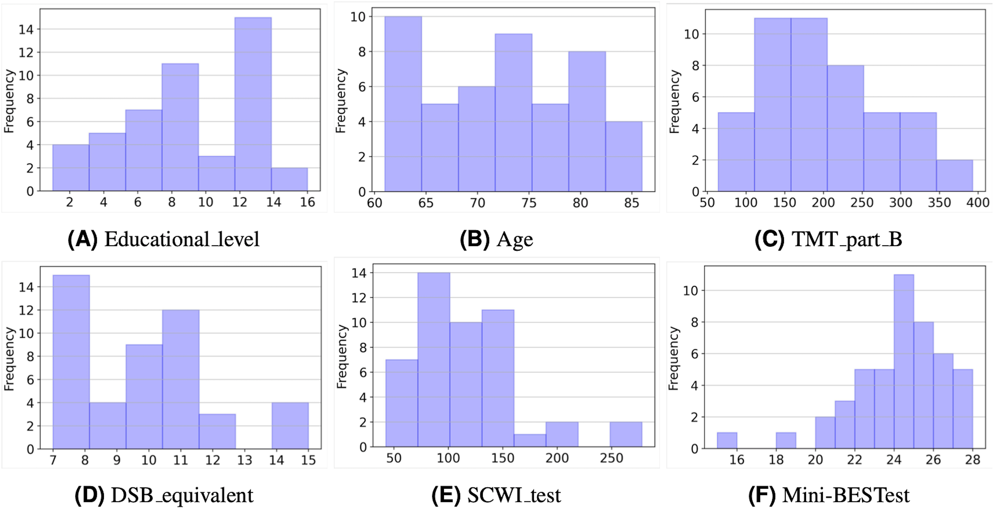
Figure 2 depicts the histograms of the six variables in the study. As can be seen, most values represent individuals with a healthy condition. For example, considering educational level (Fig. 2A), about one-third of the sample (36%) had 12 years of schooling or more, and only three subjects had more than 12 years of schooling. The average number of years of schooling was 8.6 years. With regard to the age of the selected sample (Fig. 2B), it ranges from 61 to 86 years, with an average of 72.5 years (SD:7.1).
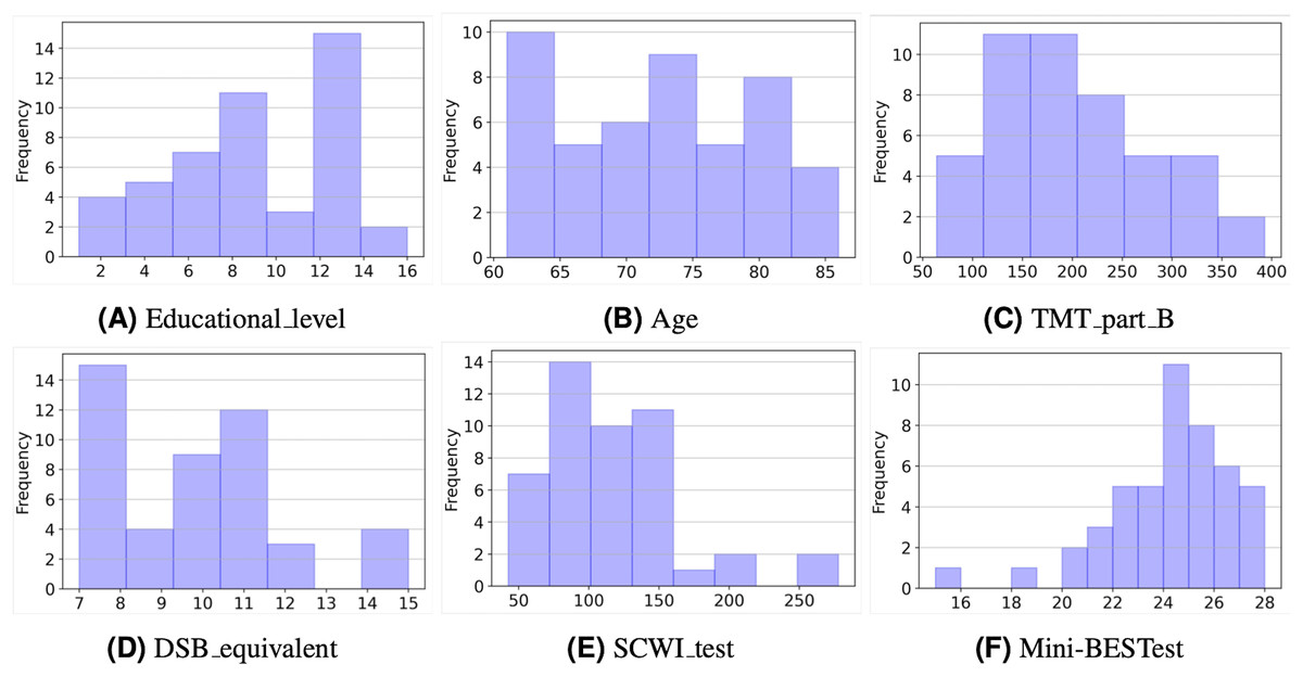
Figure 2: Histograms of the input and output variables.
As for the TMT part B values (Fig. 2C), it is interesting to note that a large part of the sample (85%) achieved times of less than 300 s. This is consistent with the normative values for this test (Arango-Lasprilla et al., 2015). In the case of the DSB (Fig. 2D), equivalent scores were considered, and 43 participants (91%) have values in the range of 7 to 13 points, which is considered average for this test (Rosas, Tenorio & Pizarro, 2012).
On the other hand, the SCWI test values (Fig. 2E) show that almost all samples (87%) achieved times of less than 150 s. According to the scale’s normative values, these are still low values considering that the times shown by the normative values are in a 50th percentile with 82 and 79 s for women and men who have a low level of schooling, respectively. Finally, Fig. 2F shows that the majority of people (74%) have values in the Mini-BESTtest above 22 points, that is, they are above the cut-off value.
Next, we carried out two additional analyses to assess the input variables’ discriminative power and the possible correlations among them. We calculated the Fisher discriminant ratio (FDR) for each input variable and the correlation matrix between them, respectively.
In Eq. (1), measures the discriminative power of the -th feature for deciding if a pattern belongs to a class or another. In this case, class 0 corresponds to a high risk of fall, and class 1 corresponds to a low risk of fall. and are the sample mean and variance of the values of the -th feature for the patterns that belong to class 0, correspondingly are and . The farther the means and the smaller the variances, the easier it is to discriminate between the classes, and FDR takes higher values. The results of FDR are depicted in Table 1. As can be seen, TMT_part_B and the Educational level are the best features for individually discriminating patterns into each class.
(1)
| Variable | FDR value |
|---|---|
| Educational_level | 0.537 |
| TMT_part_B | 0.213 |
| SCWI_test | 0.091 |
| DSB_equivalent | 0.079 |
| Age | 0.058 |
Table 2 depicts the correlation coefficients between the input variables. High values of absolute correlation imply that some variables include statistical information about others and might be redundant when predicting the output variable. We observe that three pairs of variables present an absolute correlation higher than 0,4. These pairs are TMT_part_B and SCWI_test, TMT_part_B and DSB_equivalent, and finally Educational_level and SCWI_test.
| Educational_level | Age | TMT_part_B | DSB_equivalent | SCWI_test | |
|---|---|---|---|---|---|
| Educational_level | 1 | −0.174 | −0.393 | 0.062 | −0.429 |
| Age | −0.174 | 1 | 0.199 | 0.217 | 0.148 |
| TMT_part_B | −0.393 | 0.199 | 1 | −0.480 | 0.576 |
| DSB_equivalent | 0.062 | 0.217 | −0.480 | 1 | −0.258 |
| SCWI_test | −0.429 | 0.148 | 0.576 | −0.258 | 1 |
As can be seen from Tables 1 and 2, some features are more important than others when predicting the risk of falling. At this point, we still do not discard any variables since they are few, but we use this insight to explore using different subsets of these features as input to the models. Thus, we perform a wrapper-based feature selection when assessing the classifier models.
Use of ML models with a small and imbalanced data set
Since the data set is small (47 samples), we propose using classifiers with a low number of parameters. We begin by assessing the simplest model: LR, and then we try more complex, nonlinear models like DT and K-NN. These three models are highly employed in the literature as presented in ‘Related Work’. Moving from LR to DT and K-NN did not improve models’ performance, thus we did not explore further into more complex models. We implemented the models using the scikit-learn libraries. These libraries allow setting key parameters for each classifier. The most relevant to this work is class weight, which is set for each classifier as balanced. Using balanced class weights penalizes more heavily misclassifications of the least represented class (class ). This mitigation mechanism establishes the decision surfaces of the classifier so that a small number of samples that belong to the least represented class are correctly classified, at the potential expense of a larger number of samples that belong to the most represented class being misclassified.
Additionally, other specific parameters to the models were set according to the best values that resulted from the classification metrics. For example, in the LR we set the inverse of regularization strength, C, to (we explored ); in the DT, we set the minimum number of samples to split an internal node to 15 (we explored 3, 10, and 15); and in the K-NN we set the number of neighbors to 1 (we explored 1, 2,…, 5).
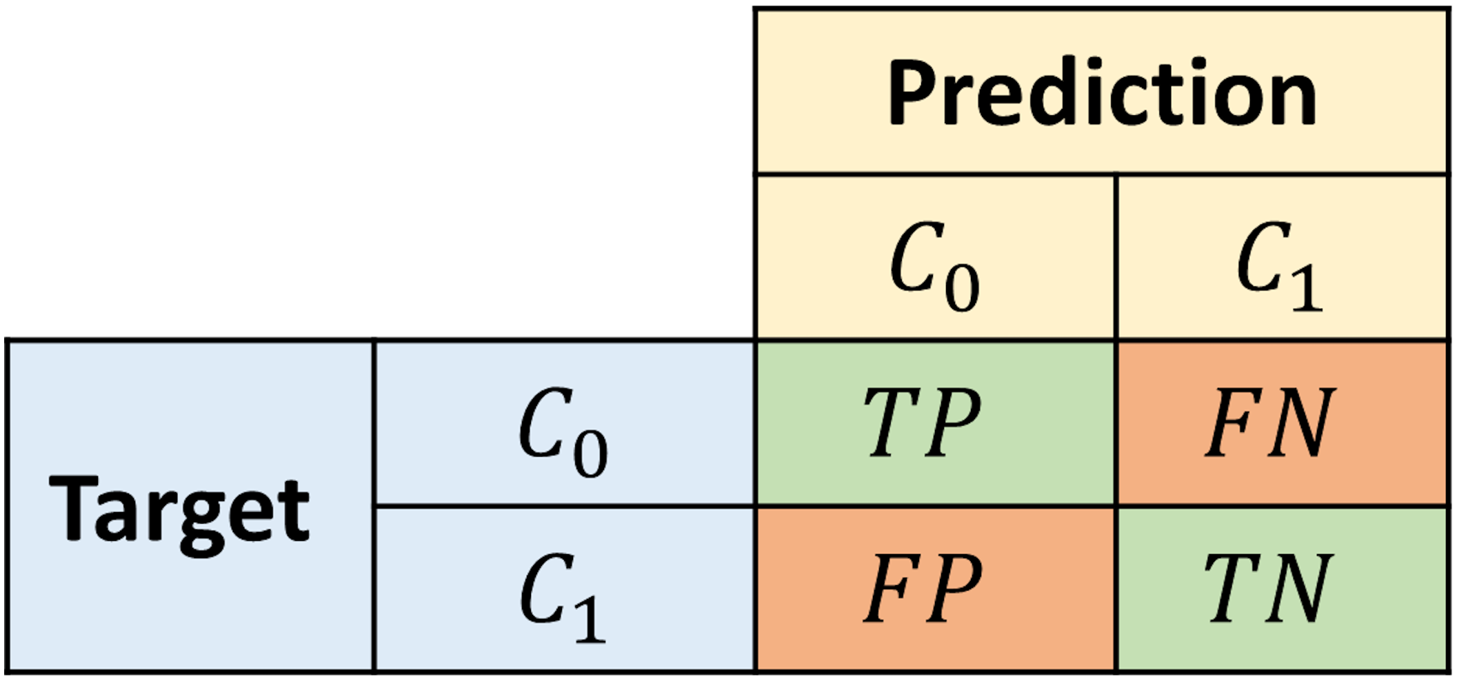
We assess the proposed models using a bootstrapping sampling method and an aggregated confusion matrix to ensure the best model performs well outside of the training data. We performed 100 evaluation experiments with different training and test sets each time. For each iteration, 70% of the samples are randomly taken as the training set and the rest is used as the test set. The latter set is employed to calculate a confusion matrix. The confusion matrices calculated in every iteration are accumulated in an aggregated matrix, representing the model’s overall performance. The structure of the confusion matrix is depicted in Fig. 3, where a sample is labeled as True positive (TP)/True negative (TN) if it belongs to the class and it is correctly classified as so. On the other hand, a sample is labeled as False negative (FN)/False positive (FP) if it belongs to the class and it is misclassified as .
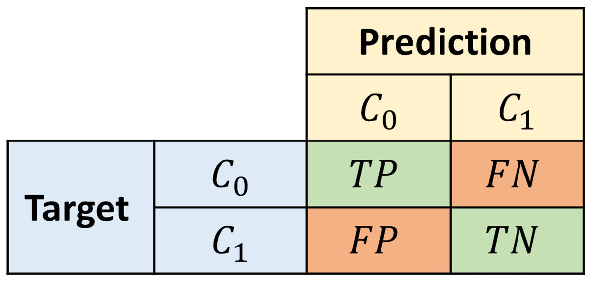
Figure 3: Structure of the confusion matrix.
To assess the proposed models, we calculate typical performance metrics (Kelleher, Mac Namee & D’arcy, 2020) on the aggregated confusion matrix. We use the accuracy and average class accuracy as overall metrics, and also four additional metrics that specify the behavior of the models predicting each class. In imbalanced data set scenarios, the average class accuracy metric is more informative than the pure accuracy since the latter might obscure the misclassifications of the least represented class. Recall- informs the percentage of all class instances correctly classified as . Meanwhile, Precision- informs the confidence that a sample classified as actually belongs to that class. Correspondingly, Recall- and Precision- convey the same information for .
Model selection
Table 3 depicts the best models obtained after assessing every combination of different sets of features as input for the proposed models. Each row contains the classifier name, the subset of features, the aggregated confusion matrix, and the metrics values. The three best models were selected via the following steps:
-
For each set of features select the model that performs the best.
-
Keep only the best-ranked models that perform similarly well.
| Model | Features | Agg. conf. matrix | Acc. | Ave. Acc. | Rec. | Rec. | Prec. | Prec. |
|---|---|---|---|---|---|---|---|---|
| LR | Educational_level | 0.714 | 0.727 | 0.745 | 0.709 | 0.305 | 0.942 | |
| LR | TMT_part_B | 0.647 | 0.606 | 0.548 | 0.664 | 0.218 | 0.896 | |
| LR | TMT_part_B, Educational_level | 0.697 | 0.676 | 0.646 | 0.706 | 0.295 | 0.913 |
Table 3 shows that the LR models have the best overall performance. The LR model with Educational_level as input achieved the best performance in every metric. A Recall- value of approximately 0.75 means that almost 75% of all individuals at risk of fall can be detected. Meanwhile, a Precision- value of approximately 0.30 indicates that when the model classifies an individual with high risk of falling, 70% of the times the individual is healthy. Therefore, the LR classifier captures the unhealthy individuals well but a follow-up might be necessary to eventually solve misclassifications. Additionally, the average class accuracy metric aggregates the ability of this classifier to detect both classes. The results of Table 3 confirm that Educational_level and TMT_part_B are the best features for discriminating individuals regarding the risk of falls, as shown by the FDR in Table 1. Next, we present a deeper analysis of the three classifiers to gain additional insight into the relationship between the input variables and the risk of falls.
LR classifier with Educational_level as input variable
First, we carried out a Wald test (Wasserman, 2013; Hastie, Tibshirani & Friedman, 2009), Eq. (2), to determine if an input variable can be dropped from the model. We tested if the mean value of the LR parameter is zero, assuming is Normal.
(2) where is the sample mean, is the estimated standard error, is the sample variance, and is the number of samples. If , where is the test size, we do not drop the parameter. A Z score greater than 1.96 in absolute value is significant at 5% level.
As seen from Table 4, in the average classifier, the Educational_level is significant. Among the 100 classifiers obtained in the experiments, we looked for the classifier that is closer to the average, obtaining Eq. (3):
(3)
| Educational_level | 0.28 | 0.13 | 0.013 | 21.5 |
| Intercept | −2.01 | 0.75 | 0.075 | 26.8 |
From this classifier, we can derive two conclusions. First, by increasing 1 year of education, the individual increases the odds of presenting a low risk of falls by 30% (exp(0.26) = 1.297). Next, when Eq. (3) is positive, the model classifies an individual as , otherwise as . Therefore, we can obtain a threshold value for the Educational_level that separates individuals with low risk of falls from those with a high risk of fall by solving , which results in a threshold value of approximately 7.5 years of education.
LR classifier with TMT_part_B as input variable
Using the Wald test for this classifier, we obtained the results depicted in Table 5. As seen in the average classifier, the TMT_part_B is significant.
| TMT_part_B | −0.01 | 0.01 | 0.001 | 10.0 |
| Intercept | 1.77 | 1.28 | 0.128 | 13.8 |
Among the 100 classifiers obtained in the experiments, we looked for the classifier that is closer to the average, obtaining Eq. (4):
(4)
From this classifier, we can derive two conclusions. First, a 1-s decrement from the TMT_part_B value increases the odds of presenting a low risk of falls by 1% (exp(0.01) = 1.010). Next, when Eq. (4) is positive, the model classifies an individual as , otherwise as . Therefore, we can obtain a threshold value of TMT_part_B that separates individuals with low risk of falls from those with a high risk of fall by solving , which results a threshold value of approximately 212 s.
LR classifier with educational_level and TMT_part_B as input variables
Using the Wald test for this classifier, we obtained the results shown in Table 6. As seen in the average classifier, both variables are significant.
| Educational_level | 0.26 | 0.15 | 0.015 | 17.3 |
| TMT_part_B | −0.01 | 0.01 | 0.001 | 10.0 |
| Intercept | −0.37 | 1.78 | 0.178 | 2.1 |
Among the 100 classifiers obtained in the experiments, we looked for the classifier that is closer to the average, obtaining Eq. (5):
(5)
From this classifier, we observe that, by holding TMT_part_B at a fixed value, the odds of presenting a low risk of falls increase by 25% (exp(0.221) = 1.247) if the years of education increase in 1 year. On the other hand, by holding the Educational_level at a fixed value, the odds of presenting a low risk of falls increases 0.6% (exp(0.006) = 1.006), if the TMT_part_B value decreases by 1 s. As the classifier presents two inputs, we cannot obtain a threshold value as in ‘LR Classifier with Educational Level as Input Variable’ and ‘LR Classifier with TMT Part B as Input Variable’. Nonetheless, in Fig. 4, we depict the classifier from Eq. (5) and its classification over all the study samples. Each point in Fig. 4 represents a sample from the study, where the coordinates are the collected values of TMT_part_B and Educational_level. The color of each point reflects its class: yellow points depict individuals with a low risk of falling (class 1), while purple points depict individuals with a high risk (class 0). The classifier separates the TMT_part_B, Educational_level plane into two half-planes. The purple half-plane is composed of points that the model classifies as class 0, and the yellow half-plane is composed of points that the model classifies as class 1. Therefore, when a sample and the half-plane it belongs to have the same color, that sample is correctly classified. Otherwise, it is misclassified.
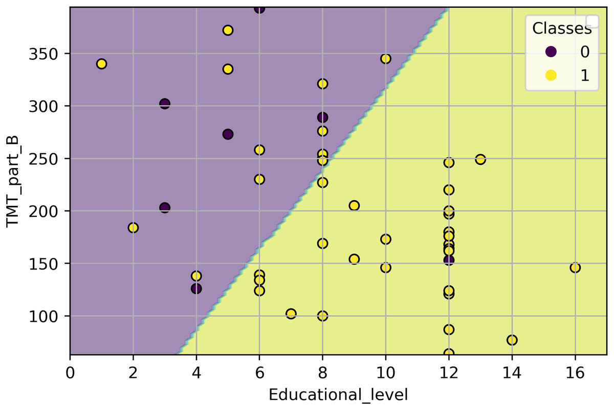
Figure 4: Classification of all study samples using the classifier from Eq. (5).
The samples are depicted using a scatter plot of the TMT_part_B and Educational_level variables.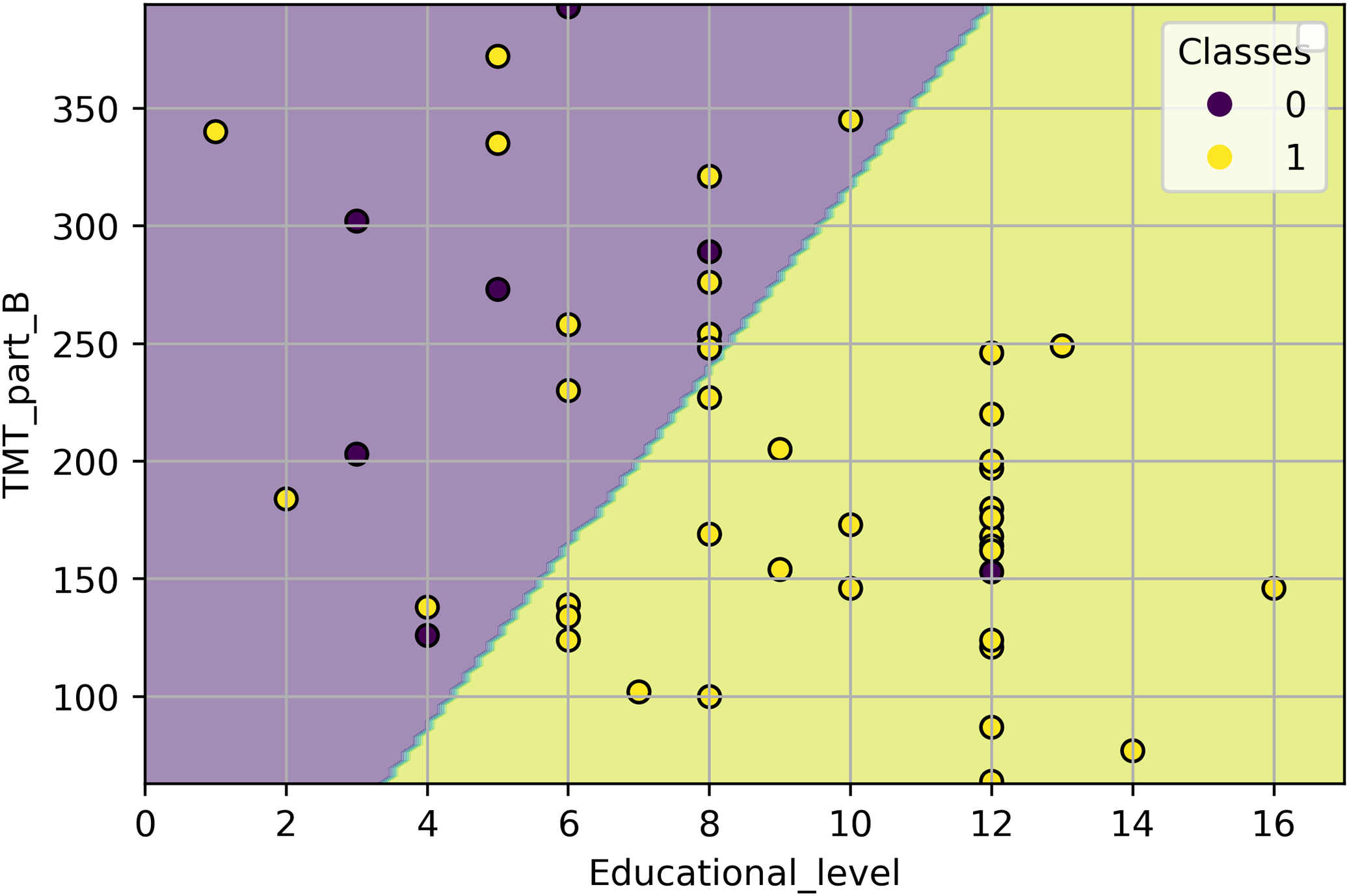
Assessing the statistical implications of the dataset sample size on the optimal model
To explore whether the couple “sample size/model complexity” of the proposed solution is good enough for the study, we have conducted a numerical experiment. From the original dataset, we extracted smaller datasets of 16, 24, 32, and 40 samples. Each dataset was produced 100 times using a bootstrapping sampling method. The 100 datasets of the same size were used to fit 100 LR models with TMT part B and Educational level as inputs, randomly selecting 70% of the samples for training and the remaining 30% for testing. We added the original dataset to this experiment (47 samples) by generating 100 different training and testing sets by bootstrapping.
We evaluate the impact of the sample size using three analyses. Firstly, we calculated the model’s average class accuracy and its 95% confidence interval on training and testing sets. We chose this performance metric because it measures the model’s ability to detect both classes and penalizes the result if one of the classes is highly misclassified. Secondly, we obtained the average effect size and its 95% confidence interval. The effect size was calculated using the values of the log odds from Eq. (5), which compares the and populations. We employed the Cohen’s d measure, which is based on the difference between means, normalized by a pooled standard deviation (Cohen, 2013). Finally, we checked the average value of the model parameters and their 95% confidence intervals.
Figure 5A depicts the average behavior of the average class accuracy for the LR model as the sample size increases from 16 to 47. The average class accuracy on the training set decreases from 0.84 to 0.77 as the number of samples increases. Meanwhile, the average class accuracy on the test set decreases when the number of samples increases from 16 to 24, and then increases from 24 to 47 samples, reaching a maximum of 0.65. In both sets, the length of the confidence intervals decreases as the sample size increases. The models trained with smaller datasets end up overfitted due to the reduced data they were exposed to and cannot generalize well. As more samples are included during the training stage, it becomes increasingly challenging to separate the classes; however, the model can better capture the underlying statistics of the data. Therefore, improving the model performance on the unseen data. Furthermore, it appears that the curves tend to values that lie between 0.77 and 0.65, which reduces possible improvements to the model to that gap, even with the addition of more data.
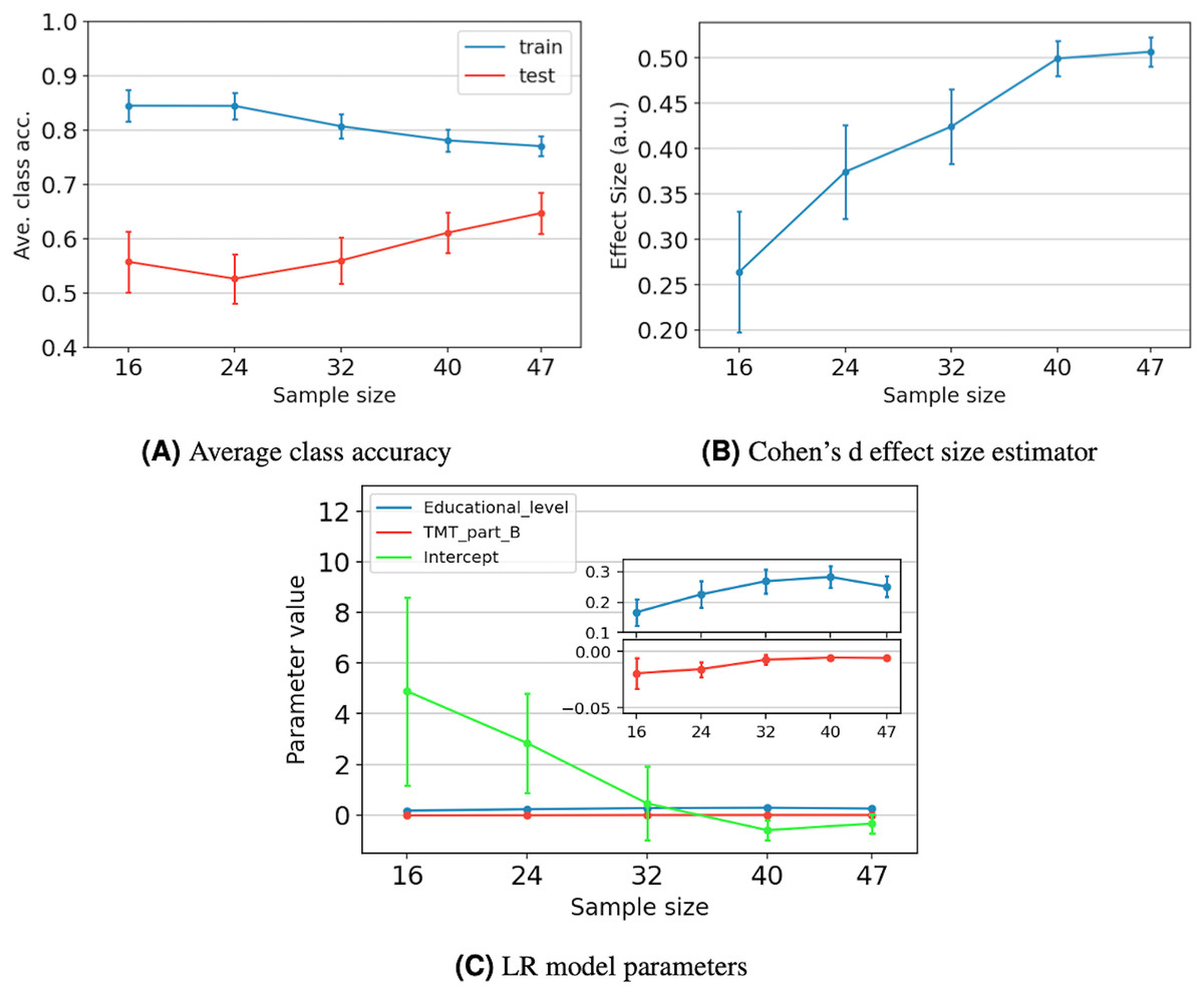
Figure 5: The impact of sample size on model performance, generalization, and stability for five different sample sizes.
For each data point, we present the average value and its 95% confidence interval. Performance and generalization are discussed through the average class accuracy (A) and Cohen’s d effect size estimator behavior (B). Meanwhile, model stability is discussed through the LR model parameters’ behavior (C). The coefficient values of the Educational_level and TMT_part_B variables are zoomed to ease their verification.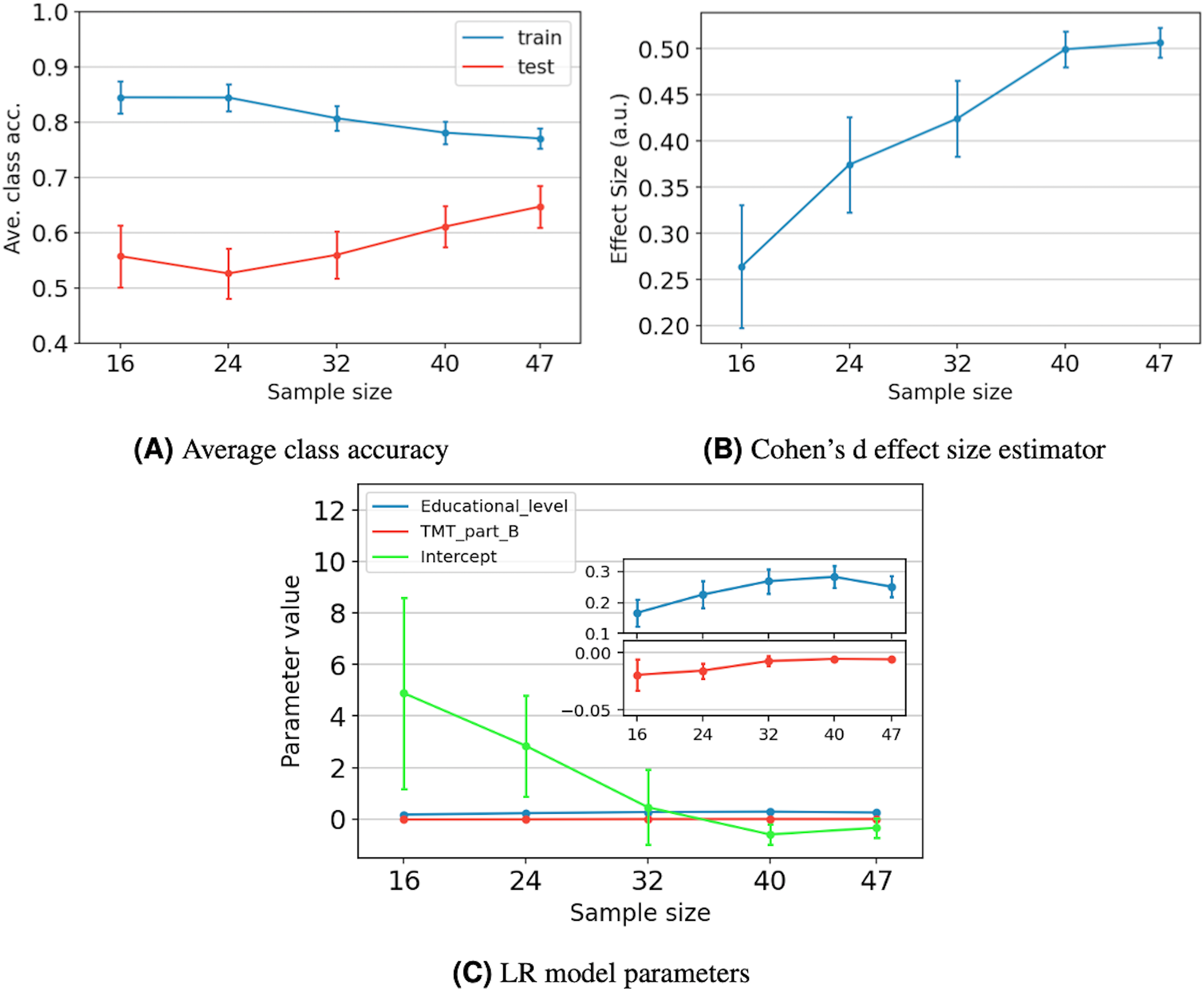
Figure 5B depicts the average effect size and its 95% confidence interval as the sample size increases. We observe that the effect size increases as the sample size increases, reaching a maximum value of 0.51. According to Cohen (2013), an effect size of 0.5 is considered moderate, indicating a medium resolving power between the two classes. Specifically, it indicates that the difference between classes means equals half a standard deviation. Additionally, we observe that increasing the sample size from 40 to 47 results in a gain of only 0.01 in the effect size.
Figure 5C shows the average value of the LR model parameters as the sample size increases. We observe that the average values present a tendency towards specific numbers, which appear to stabilize after 40 samples. Additionally, for the three parameters, the length of the confidence intervals decreases as the sample size increases. Just as in the average class accuracy analysis, including more samples during the training stage allows the model to better capture the underlying statistics of the data, resulting in more robust parameters.
Discussion
So far, our results show that TMT_part_B and Educational_level can be used to identify community-dwelling older adults at high risk of falls. Next, we discuss our results and point out the findings’ reach and limitations.
The first hint to identify the strongest predictors for the risk of falls was obtained by the data analysis carried out in ‘Output Variable Binarization’. Table 1 shows that, individually, TMT_part_B and Educational_level are the best features for discriminating individuals with high risk of falls. This result is supported by the top-ranked ML models presented in Table 3, which included one or both features as inputs. While other studies have recognized the potential of the TMT as a tool for detecting fall risk (Sturnieks et al., 2025), most of the evidence comes from traditional statistical analyses (Kang et al., 2017) and focuses mainly on motor or demographic predictors (Ikeda et al., 2022; Jehu et al., 2021).
Additionally, Table 2 depicts the correlation coefficients between the features. The high correlation between the variables associated with the cognitive tests indicates that some of them could be redundant for the ML model. In the literature, other authors have defined multiple subdomains (Laakso et al., 2019) and a series of tests to assess them (Goldstein & Naglieri, 2014). Miyake et al. (2000) have focused their studies on the assessment of three of them, i.e., shifting, inhibition, and updating, which can be fully assessed by the TMT part B, SCWI, and DSB tests, respectively. Nonetheless, we observed through the correlation analysis that the variable TMT_part_B includes much of the information that the DSB_equivalent and SCWI_test provide. This conclusion can also be verified by the results obtained when using these cognitive tests to identify the risk of falls through ML models in ‘Model Selection’.
In ‘Model Selection’, we present the best ML models to identify older adults with a high risk of falls. Table 3 depicts the top-ranked models obtained in our study and their performance. In our work, we employed balanced class weights to mitigate class imbalance. Such a mechanism affects some performance metrics positively, and others negatively. Its effect is larger the more mixed the classes are in the feature space (see Fig. 4). Using balanced class weights compared to not using them increases the number of TP samples a little, while TN samples decrease by a larger amount. The latter causes FN samples to decrease, and FP samples to increase. Therefore, Recall- , Precision- , and the average class accuracy metrics increase, while the accuracy, Recall- , and Precision- decrease. Furthermore, using balanced class weights might potentially increase the chances of overfitting, particularly given the number and distribution of samples of the least represented class in the feature space. If there are few samples and they are too spread out, the model during the training stage could establish decision surfaces based on a distribution of samples that would be too different from the unseen samples at the test stage.
According to the metrics in Table 3, the LR model with the educational level as input is the best classifier. Nonetheless, such a model is very coarse-grained. From a clinical perspective, it is incorrect to use the educational level as the sole factor in keeping a good balance in older people (Lathouwers et al., 2022; Lee et al., 2021). A more suitable model is the LR model, with TMT_part_B and Educational_level as inputs. The performance of this classifier is slightly lower, but it allows us to consider a broader range of clinical information and derive more conclusions than the first mentioned. For example, in Fig. 4, we can observe that for a specific Educational_level, lower values of the TMT_part_B test are associated with individuals who present a lower risk of falling. Meanwhile, high values of TMT_part_B indicate that an individual presents a higher risk of falling. On the other hand, for a specific value of the TMT part B test, more years of education are associated with a lower risk of falling. The above is consistent with the results of Voos, Custódio & Malaquias (2021), who describe an association between the occurrence of falls, years of education, and executive function.
The LR model described in Eq. (5) delivers additional insights into the relationship between the features and the risk of falls. If different treatments improve TMT_part_B or Educational_level differently and there is a way to quantify this improvement, then one of those treatments can be selected to maximize the value of Eq. (5), thus maximizing the odds of presenting a low risk of falls. Therefore, besides detecting the current medical condition of individuals, the model could be used to improve such conditions by selecting a more suitable treatment.
Regarding the sample size of the study, we acknowledge that it is small compared with typical ML scenarios. Nonetheless, the quality of a dataset should be assessed by its impact on model performance, generalization, and stability, rather than the number of samples it contains. According to Figs. 5A and 5B, the model stabilizes after 40 samples, and little improvement in effect size is observed by moving forward to 47 samples. In a similar study to ours, Rajput, Wang & Chen (2023) proposed two criteria for selecting a suitable sample size. Firstly, the average effect size should be equal to or more than 0.5, according to Cohen’s scale. Secondly, the change in the performance metric should be smaller than 10%, from the assessed sample size to the next. For 40 samples, the average effect size is 0.5, and the change in average class accuracy is 4%. For 47 samples, the average effect size is equal to 0.51. Supposing that, for a larger sample size, the average class accuracy on the test set would be around 0.71, which is in the middle of 0.77 and 0.65 (gap between training and testing, see ‘Assessing the Statistical Implications of the Dataset Sample Size on the Optimal Model’). Then, the change in average class accuracy would be 8%. Therefore, both sample sizes are statistically significant to build the LR model. Including more data might benefit the model, but only to a limited extent.
Table 7 compares, in terms of ML performance metrics, four assessment tools reported by Yingyongyudha et al. (2016), with the proposed model obtained in our work (LR described in ‘LR Classifier with Educational Level and TMT Part B as Input Variables’). Older adults were recruited in the aforementioned study from an urban community, similar to our study. As can be seen, our classifier is the second in AUC and Recall- , only behind Mini-BESTest. Meanwhile, it is the third in accuracy, and fourth in Recall- . In general, its performance is closer to BESTest.
| Assessment tool | AUC | Recall- (Sensitivity) | Recall- (Specificity) | Accuracy |
|---|---|---|---|---|
| Mini-BESTest | 0.84 | 0.85 | 0.75 | 0.85 |
| BESTest | 0.74 | 0.76 | 0.50 | 0.76 |
| Our work | 0.78 | 0.65 | 0.71 | 0.70 |
| BBS | 0.69 | 0.77 | 0.42 | 0.60 |
| TUG | 0.32 | 0.40 | 0.34 | 0.65 |
From a practical point of view, it is reported that BBS is known for having ceiling effects, and TUG only measures one sequential task of walking and turning, ruling out other factors involved in falls (Yingyongyudha et al., 2016). On the other hand, the primary disadvantage of BESTest is that it requires 20 to 30 min to administer (Horak, Wrisley & Frank, 2009), whereas Mini-BESTest requires about 15 min (Godi et al., 2013). Our model, which considers TMT part B together with educational level, can be a relevant tool for assessing the risk of falling in non-specialized contexts, given that it achieves adequate values in predictive performance indicators such as accuracy and AUC. Furthermore, TMT part B takes less than 6 min to complete (Waggestad et al., 2025) and only requires a pencil and paper, without needing additional physical space or specialized equipment.
Our study presents some limitations that will be covered in future work, and we mention them below. First, our results are focused on the community-dwelling older adult population. To generalize our results beyond this population, we need to recruit older adults from diverse socio-demographic characteristics, as these characteristics are strongly correlated with the risk of falls in this age group (Lathouwers et al., 2022). Second, the study had a small number of participants. We note that some works in the state-of-the-art also analyze small datasets (Roshdibenam et al., 2021; Shumway-Cook, Brauer & Woollacott, 2000). Nonetheless, we understand that a larger dataset would allow to train more complex ML models and employ more robust methodologies such as cross-validation. Third, the number of features considered in the study design was small: only five. In future work, we plan to add more cognitive tests to our model to search for additional relationships between cognitive functions and falling risk. Also, we plan to include variables related to sociodemographic characteristics, comorbidities, and different medical conditions to assess how much they improve model performance when combined with cognitive functionality.
Conclusions
In this work, we developed an LR classifier to identify older adults with high or low risk of falling, using TMT part B test and the educational level as features. The study followed a typical ML methodology, which included the following steps: First, data collection, cleaning, and analysis. Second, setting up ML models of different nature, such as LR, DT, and K-NN using a small and imbalanced data set. Finally, we trade off performance metrics and clinical analysis to select the best model.
The study initially considered five input variables: the educational level, age, TMT part B, DSB, and SCWI, which underwent a wrapper-based feature selection. Only TMT part B and the educational level remained in the best model. The correlation and FDR analyses foresaw this result. Thereby, out of the three executive function tests, TMT part B is enough to assess the risk of falls. We weigh the performance metrics results with a clinical perspective to determine the best model. Even though the LR with TMT_part_B and Educational_level as inputs presents slightly lower performance metrics than the top-ranked, it offers a broader range of clinical information and allows for more conclusions. Finally, we mention that the best LR classifier allows us to quantify how changes in the input variables improve the detection of adults with a risk of falls. Suppose a set of treatments exists, and we can measure how they improve the TMT_part_B and Educational_level variables. In that case, we can use the classifier to select the treatment that maximizes the odds of presenting a low risk of falls after applying the treatments. We analyzed two more classifiers that only consider one input variable. These models allow determining a cut-off value for the input variable to identify older adults at risk of falling. We found that, individually, 8 years or more of schooling or a result of the TMT part B lower than 212 s are associated, on average, with a low risk of falls.
The study expands the state-of-the-art in fall-risk assessment and confirms that education level and TMT part B are strong predictors of fall events. Furthermore, data-driven models can capture the relationship between cognitive domain factors and the risk of falls in older adults.
Future efforts to improve the proposed model include increasing the number of participants in our study and generalizing our results to populations beyond the community-dwelling older adult population. A larger dataset would allow to employ more robust methodologies such as cross-validation and more advanced models. We plan to include more variables in the study, such as socio-demographic characteristics, cognitive tests, physical well-being, and medical conditions.
Supplemental Information
Six variables dataset.
The values of six variables collected from 50 community-dwelling older adults. The variables included age, educational level, and TMT part B, Digital Span Backward, Stroop Color-Word Interference, and Mini-BESTest tests.
Python Code and data of the different algorithms implemented.
Executive Function and Postural Balance Tests - Spanish.
Empty copy (in Spanish) of the questionnaires we used in this study.
Executive Function and Postural Balance Tests - English.
Empty copy (in English) of the questionnaires we used in this study.