
Optimizing PROAFTN classifier with ant colony algorithm: enhanced diabetes detection benchmarking
- Published
- Accepted
- Received
- Academic Editor
- Bilal Alatas
- Subject Areas
- Algorithms and Analysis of Algorithms, Artificial Intelligence, Data Mining and Machine Learning, Optimization Theory and Computation, Neural Networks
- Keywords
- Fuzzy classification, Ant colony optimization, Multicriteria classification, Machine learning, Metaheuristics
- Copyright
- © 2025 Al-Obeidat
- Licence
- This is an open access article distributed under the terms of the Creative Commons Attribution License, which permits unrestricted use, distribution, reproduction and adaptation in any medium and for any purpose provided that it is properly attributed. For attribution, the original author(s), title, publication source (PeerJ Computer Science) and either DOI or URL of the article must be cited.
- Cite this article
- 2026. Optimizing PROAFTN classifier with ant colony algorithm: enhanced diabetes detection benchmarking. PeerJ Computer Science 12:e3363 https://doi.org/10.7717/peerj-cs.3363
Abstract
The increasing global prevalence of diabetes highlights the need for accurate diagnostic tools to improve early detection and effective treatment planning. Traditional classification models often struggle to achieve optimal performance due to limitations in parameter tuning and adaptability to complex datasets. To address these limitations, this article introduces PROAnt, an innovative learning approach designed to enhance the robustness and efficiency of the PROAFTN multicriteria classification method. PROAnt leverages the computational power of ant colony optimization (ACO) to dynamically fine-tune and optimize the key parameters, such as intervals and weights, at the core of the PROAFTN classification process. This learning methodology is crucial because PROAFTN depends on these parameters for classification. ACO, inspired by the foraging behavior of ants, achieves rapid and accurate convergence with minimal parameters, outperforming many traditional optimization techniques. This study demonstrates how ACO can inductively infer PROAFTN’s parameters from data, leading to high accuracy and precision. Evaluations were conducted on a publicly available diabetes dataset containing 100,000 samples, sourced from Kaggle’s 2023 machine learning competition. This dataset includes demographic and clinical features, providing a robust basis for model benchmarking. The model achieved a classification accuracy of 98.42%, along with a weighted precision of 83.73%, a weighted recall of 0.789, and a weighted kappa of 0.789 ± 0.008, outperforming other baseline classifiers such as a feedforward deep neural network (three hidden layers: 128, 64, 32), decision trees, k-Nearest Neighbors (k-NN) and logistic regression. These findings underscore the transformative potential of integrating ACO with PROAFTN, not only in advancing diabetes detection but also in the broader application of artificial intelligence.
Introduction
Classification is a fundamental aspect of machine learning (ML) and artificial intelligence (AI), focusing on building reliable models to uncover complex patterns in data. The ultimate goal is to accurately assign unseen instances to predefined categories, which makes classification a vital tool for automating the decision-making process and effectively managing data (Bishop, 2006; Friedman, Hastie & Tibshirani, 2001; Kotsiantis, Zaharakis & Pintelas, 2007). An example of a classification application includes image recognition, where algorithms can classify images into different categories, such as identifying objects or recognizing facial expressions. In natural language processing (NLP), text classification algorithms can categorize documents into various topics or sentiment categories, aiding in spam detection, sentiment analysis, and document organization. Various classification algorithms have been developed over the years, ranging from symbolic methods like decision trees (Quinlan, 1993) and rule-based systems (One-R) (Holte, 1993) to statistical models such as Naive Bayes (Mitchell, 1997) and logistic regression, as well as neural networks (Mitchell, 1997) and instance-based learning approaches like k-Nearest Neighbors (k-NN) (Mitchell, 1997). These models, while effective in many scenarios, often struggle when dealing with vague or uncertain common characteristics of real-world medical datasets (Friedman, Hastie & Tibshirani, 2001; Mitchell, 1997).
In addition, classification is crucial in medical diagnosis, fraud detection, and customer segmentation. In medical diagnosis, machine learning models can analyze patient data, such as symptoms, medical history, and test results, to classify individuals into specific disease categories. In fraud detection (du Preez et al., 2025), classification algorithms analyze patterns in financial transactions to identify potentially fraudulent activities. Customer segmentation involves classifying customers into distinct groups based on their behaviour, preferences, or demographics to tailor marketing strategies (Amin, Adnan & Anwar, 2023).
On the other hand, multiple-criterion decision analysis (MCDA) (Triantaphyllou, 2000) has gained popularity as an alternative approach to decision-making (Triantaphyllou, 2000) and classification tasks. Initially conceived in operations research, social psychology, and business management, MCDA techniques are gaining momentum in healthcare, data mining, and business (Belton & Stewart, 2002). The classification problem within the MCDA framework involves using prototypes to assign objects to classes, with each prototype representing a distinct class based on a set of attributes (Belacel, Wang & Richard, 2005; Hwang & Yoon, 1995). On the other hand, PROAFTN was introduced and developed in original form by Belacel (1999, 2000), as a multicriteria assignment/classification method with fuzzy interval prototypes; later works extended learning procedures and applied PROAFTN in diverse domains such as education (Al-Obeidat et al., 2018), and e-health (Belacel, Wang & Richard, 2005). It utilizes the MCDA paradigm to enhance understanding of the problem domain and provides direct techniques that enable a decision maker (DM) to adjust its parameters. As a transparent classification method, the fuzzy approach of PROAFTN allows for detailed insights into the classification decision (Al-Obeidat & El-Alfy, 2019). However, PROAFTN requires the prior determination of multiple parameters, such as interval boundaries, weights, and preference thresholds. The decision problem is formulated using prototypes, each representing a distinct class, to categorize each object into its appropriate category. In an MCDA framework, these parameters largely depend on the DM’s judgment, which sets the ’boundaries’ of the attributes and the weights based on their evaluation. Moreover, the manual adjustment of the PROAFTN parameters limits its adaptability and scalability, especially in complex datasets such as those used for diabetes detection. Although several previous studies (Al-Obeidat et al., 2009, 2010, 2011) have investigated the use of metaheuristic algorithms such as Genetic Algorithm (GA), Differential Evolution (DE), and Particle Swarm Optimization (PSO) to optimize PROAFTN, comparatively limited attention has been devoted to ant colony optimization (ACO) (Dorigo, Maniezzo & Colorni, 1996)—a powerful bio-inspired technique renowned for its ability to efficiently explore large search spaces and avoid premature convergence to local minima. To my knowledge, this is the first fuzzy classification framework based on ACO that dynamically learns the PROAFTN parameters for medical diagnosis (Dorigo & Blum, 2006; Dorigo & Stützle, 2004). ACO has found significant applications in the training of neural networks (NN) (Kaya et al., 2023; Blum & Li, 2008). Traditional NN training techniques, such as gradient descent, often suffer from local minima problems. ACO offers an alternative, effective means to traverse the solution space and escape local minima, resulting in potentially better network parameters and improved performance. ACO has also been applied in decision-making and game-playing scenarios. For example, ACO is used in reinforcement learning environments for strategies in game playing (Sharma, Kobti & Goodwin, 2008; Liao, Wang & He, 2018).
Several notable studies have explored classification through interval learning and feature representation. Dayanik (2010) proposed algorithms based on feature interval learning that provide robust classification by handling uncertainty in input features. De Chazal, O’Dwyer & Reilly (2004) used interval features in electrocardiogram (ECG) morphology for heartbeat classification, demonstrating strong performance in medical diagnostics. Demiröz & Güvenir (1997) introduced a voting mechanism over feature intervals, which inspired more interpretable classifiers. In a related medical application, Güvenir & Emeksiz (2000) built an expert system based on feature intervals for disease diagnosis. Recently, Belacel (2025) proposed a Closest Similarity Classifier using classification and interval learning, showing improved performance in classification tasks. These prior studies reinforce the value of interval-based learning, which our proposed PROAnt model builds upon by using fuzzy intervals and metaheuristic optimization through ACO.
Recent studies have explored the use of bio-inspired algorithms for medical classification problems. Recent advancements in intelligent classification systems have explored the integration of deep learning with metaheuristic optimization to enhance performance. Abgeena & Garg (2023) proposed a hybrid S-LSTM-ATT model combined with Firefly Optimization for emotion recognition from EEG signals, achieving high classification accuracy on complex biomedical data. Their work highlights the potential of combining deep temporal models with optimized feature selection to address nonlinear and noisy datasets in health informatics. In contrast, our study focuses on a transparent, interpretable fuzzy multicriteria classification framework enhanced by ACO, offering an alternative approach for accurate and explainable medical diagnosis, particularly for diabetes detection.
To bridge this gap, we propose PROAnt, a novel classification framework that integrates ACO with the PROAFTN classifier. In PROAnt, ACO serves as an inductive learning mechanism that automatically infers the key fuzzy parameters—intervals and weights—from data. This eliminates the need for manual configuration and significantly enhances the model’s robustness, adaptability, and performance. Unlike conventional optimization strategies, ACO simulates the pheromone-guided behavior of ants to explore the solution space efficiently, allowing the model to discover high-quality classification rules through an iterative learning process. The learned prototypes and associated rules are then used to classify unseen instances with greater precision and interpretability.
The propose PROAnt, a novel methodology that uses ACO as an inductive learning mechanism to optimize PROAFTN parameters directly from data. PROAnt, leverages ACO’s capabilities to train and enhance the PROAFTN classifier. This approach uses ACO as an inductive learning mechanism to extrapolate the optimal PROAFTN parameters from the training dataset. These derived parameters are subsequently used to form the classification model prototypes. We propose PROAnt, a novel methodology that uses ACO as an inductive learning mechanism to optimize PROAFTN parameters directly from data. These derived parameters are subsequently used to form the classification model prototypes. The novel objectives of this study are: (i) introducing ACO as an inductive mechanism for optimizing PROAFTN parameters, (ii) evaluating PROAnt on a large-scale diabetes dataset, and (iii) benchmarking against multiple classifiers to validate improvements in accuracy and interpretability. Despite the use of metaheuristics such as GAs and PSO to enhance PROAFTN, no prior study has integrated ACO to dynamically learn fuzzy intervals and attribute weights for medical diagnosis. Furthermore, limited attention has been paid to balancing interpretability and accuracy in PROAFTN-based classifiers. These gaps motivate this proposed PROAnt framework.
The structure of the remainder of this article is as follows: ‘PROAFTN Method’ provides a brief overview of the PROAFTN method and the ACO algorithm. ‘Meta-Heuristic Algorithms Developed for Enhancing Proaftn Learning’ introduces the proposed PROAnt approach for learning PROAFTN-based ACO. ‘Application and a Comparative Study’ describes the data sets, the experimental results, and the comparative numerical studies. Finally, ‘Conclusions and Future Work’ discusses the conclusions drawn and proposes directions for future research.
PROAFTN method
This section details the PROAFTN classification method, which is grounded in the principles of supervised learning algorithms and is notably distinguished by its reliance on fuzzy approaches to address classification tasks. PROAFTN operates by establishing fuzzy relations between classified objects and prototype classes to determine a degree of membership linking these objects to the problem classes (Belacel, 2000).
PROAFTN’s fuzzy-based methodology augments its classification precision and fosters a deeper understanding of the problem domain, crucial in numerous real-world applications. Among these, it has been used to solve complex problems in various fields such as medical diagnostics (Belacel & Boulassel, 2001), asthma treatment (Sobrado et al., 2004), cervical tumor segmentation (Resende Monteiro et al., 2014), Alzheimer’s diagnosis (Brasil Filho et al., 2009), e-Health (Belacel, Wang & Richard, 2005), and even in the intricate domain of optical fiber design (Sassi, Belacel & Bouslimani, 2011).
Furthermore, PROAFTN has been adopted in cybersecurity, effectively used for intrusion detection and analysis of cyberattacks (El-Alfy & Al-Obeidat, 2015, 2014). In particular, the work of Singh & Arora (2015) stands out, where PROAFTN was applied to detect network intrusion. Their results attest to the superior performance of PROAFTN compared to the well-established SVM classifier (Singh & Arora, 2015).
Recently, Al-Obeidat et al. (2015) successfully used PROAFTN in image processing and classification. This underscores PROAFTN’s versatility and robustness, cementing its position as an effective solution to various classification problems that demand high accuracy and interpretability. This article elucidates the parameters required for the PROAFTN classification methodology and delineates the process and procedure that PROAFTN adopts for its classification tasks.
PROAFTN notations
Table 1 summarizes the PROAFTN notations used in this study, clearly understanding the mathematical symbols and variables integral to the PROAFTN method.
| A | Set of objects for classification |
| Set of attributes: | |
| Set of classes: | |
| Prototype set for category: | |
| B | Set of all prototypes: |
| , | Interval of for in , |
| , | Preference thresholds for for in |
| Weight for in |
In the context of the PROAFTN method, these notations quantitatively represent the objects to be classified, the defining attributes, the prototypes for each class, and the preference thresholds and attribute weights within each category. Together, these elements form the mathematical framework that underpins the PROAFTN classifier and allows its effective operation.
Fuzzy intervals
Fuzzy intervals are crucial in data mining, particularly in the rule-induction process. Standard data mining systems, such as those for rule induction and decision tree construction, discretize numerical domains into intervals when dealing with both numerical and nominal attributes. The resultant discretized intervals are then processed like nominal values during the rule induction phase. This document introduces a type of fuzzy interval used in the HCV version 2.0 rule-induction software, which helps interpret rule-induction outcomes when rules with sharply defined intervals cannot provide a precise application path for a given test example. The utility of these fuzzy intervals is underscored by a series of experimental results obtained through the application of HCV.
Assuming a set of objects, denoted as a training set, we consider an object that is yet to be classified. This object is characterized by a set of attributes , and is to be classified into one of classes . The procedure is broken down into the following steps:
For each class , a set of prototypes is identified. For every prototype and each attribute , an interval , is specified such that . The introduction of two thresholds, and , allows us to define the fuzzy intervals: the pessimistic interval and the optimistic interval . Optimistic assessments reduce the strictness of the interval boundaries, thereby narrowing the gap between the borderline and typical cases. For example, a slightly elevated glucose level can still contribute to positive membership in the diabetic class under the optimistic view, improving sensitivity.
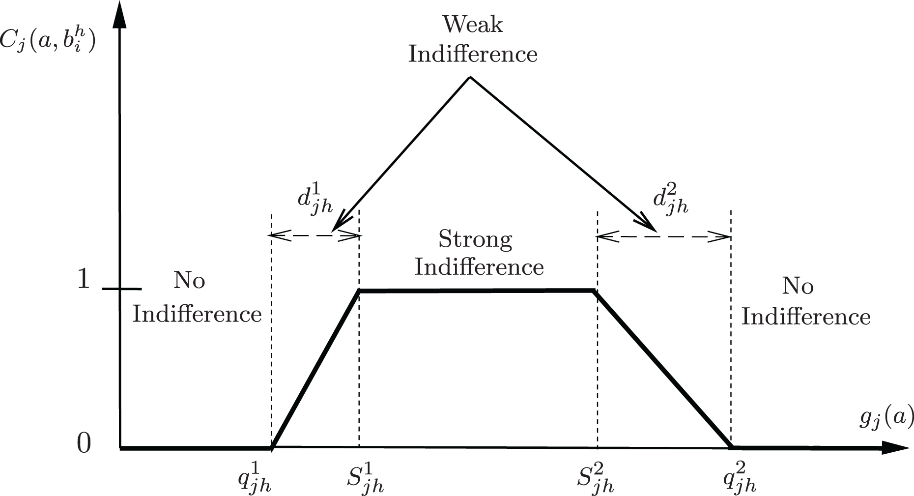
Figure 1 visually presents the interval representation within PROAFTN. For the implementation of PROAFTN, both the pessimistic interval and the optimistic interval (Belacel, Raval & Punnen, 2007) for each attribute in each class. Figure 1 also underscores the importance of avoiding extreme cases in evaluating specific measures or quantities with a crisp interval, namely, overestimating or underestimating the interval. Using crisp intervals risks excluding borderline patients or overfitting to outliers. By avoiding extreme cases and employing fuzzy intervals, PROAFTN ensures a balance between conservative and optimistic assessments, enabling more robust medical predictions.
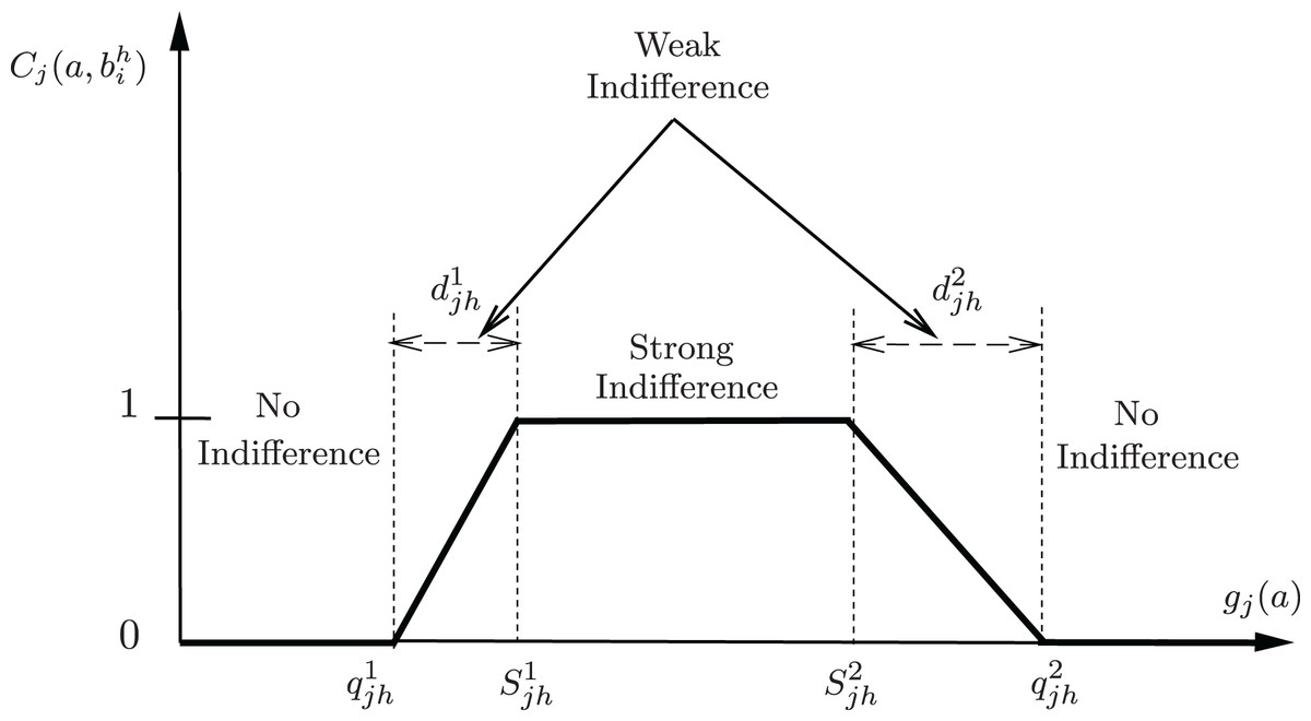
Figure 1: Graphical representation of the partial indifference concordance index between object a and the prototype b represented by intervals.
In contrast, a pessimistic evaluation can widen the interval, leading to a conservative estimate that might overlook some potentially significant observations. However, an overly optimistic assessment can narrow the gap, potentially managing outliers and leading to excessively narrow generalizations.
Therefore, PROAFTN employs fuzzy intervals to balance pessimistic and optimistic extremes. This allows for a more nuanced evaluation that can effectively handle the uncertainty and vagueness present in the data. The adoption of fuzzy intervals in PROAFTN accommodates a broader range of values, enhancing its applicability and flexibility in different contexts. In addition, these intervals are determined based on expert knowledge or data-driven methods, strengthening the interpretability and robustness of the model.
In the context of the implementation of PROAFTN, the fuzzy intervals provide a more dynamic representation that accommodates the inherent uncertainties and variations within the data, thus creating an adaptable and resilient model. This nuanced approach further bolsters PROAFTN’s ability to handle complex classification tasks and yield insightful results effectively.
(1a)
(1b) applied to:
(2a)
(2b)
Hence, = , = , = , = , = , and = . The following subsections explain the stages required to classify object to class using PROAFTN. Here, denote lower and upper fuzzy bounds for attribute j in class h; and are expansion thresholds; wjh represents attribute weights. Together, these parameters define class prototypes and guide membership calculation.
In this way, the performance matrix captures the comparative relationship between each attribute of the object and the corresponding attribute in each prototype from each class . This comparison based on individual attributes facilitates a detailed and comprehensive evaluation of the object’s relationship with the prototypes, further aiding the subsequent classification process.
As a note, the degree of partial fuzzy indifference is a number that falls within the range [0, 1], where 0 indicates no similarity between the attribute value of the object and the prototype, and 1 indicates complete similarity or ‘indifference’ A value between 0 and 1 indicates partial similarity or ‘weak indifference.’
To illustrate this process, let us consider a hypothetical case where we have a set of attributes and two prototypes and , from the same class. If we denote the attribute values for object by , the calculation of the degree of partial fuzzy indifference between object and each prototype would be carried out as follows:
For prototype , we calculate , , and based on attribute values , , and respectively. Similarly, for prototype , we calculate , , and .
This process is repeated for all prototypes across all classes, resulting in a comprehensive performance matrix that contains the degree of partial fuzzy indifference for each prototype against each attribute of the object .
Once the performance matrix is calculated, the next step in the classification process involves calculating the total fuzzy indifference relation for each prototype, which involves a weighted summation of the individual attribute-based fuzzy indifference degrees as given by Eq. (5).
Applying the fuzzy indifference concept within the framework of the PROAFTN algorithm allows effective handling of uncertainty, making it a potent tool for tackling complex classification tasks in areas such as data mining and machine learning.
Calculation of the fuzzy indifference relation:
The classification procedure begins with the computation of the fuzzy indifference relation, . This is a concept derived from the principles of concordance and non-discordance, serving to quantify the relationship, or the degree of membership, between an object to be assigned and a prototype (Belacel, 1999; Belacel, Raval & Punnen, 2007). The fuzzy indifference relation is formulated as follows:
(3)
Here, is the weight that signifies the relevance of an attribute for a specific class and is constrained as follows:
The term denotes the degree to which the object is close to the prototype based on the attribute and is computed as:
(4) where
and
The discordance index, , measures the dissimilarity between the object and the prototype based on the attribute . This index employs two veto thresholds and (Belacel, 2000). The object is considered perfectly distinct from the prototype if the attribute reaches these veto thresholds. However, as defining veto thresholds via inductive learning can be risky and requires expert input, this study focuses on an automatic approach, thus setting the veto thresholds to infinity, effectively eliminating their impact. As a result, the computation simplifies to relying solely on the concordance principle, which can be expressed as:
(5)
Three comparative scenarios between object and prototype based on attribute can be outlined (Fig. 1):
-
Strong Indifference:
; (i.e., )
-
No Indifference:
, or
-
Weak Indifference:
The value of is derived from Eq. (4). (i.e., or )
The study and application of such functions are well documented in Marchant (2007) and Ban & Coroianu (2015).
By encapsulating the concept of fuzzy indifference, the PROAFTN classification algorithm adeptly manages the inherent uncertainty in data, providing a robust solution to complex classification tasks in fields such as data mining and machine learning.
Estimation of membership degree:
To determine the degree of membership, , between an object and a class , the PROAFTN classification algorithm takes advantage of the degrees of difference between and its closest prototype within the class . This approach helps to quantify the degree to which the object aligns with a specific class based on its similarity to its representative prototypes.
The determination of the nearest prototype is achieved through an exhaustive comparison of the indifference degrees of with all prototypes within . Thus, the maximum indifference degree acquired will denote the most similar or ‘nearest’ prototype. This can be mathematically represented as:
(6)
The resultant measures the object’s affinity to class , a higher value indicating a stronger association.
Classification of an object: assignment to the appropriate class
Upon computing the membership degrees between the object and all classes, the final step is to assign to the class that maximizes this degree. This step effectively assigns the object to the class with the highest similarity based on the calculated indifference degrees.
The assignment is executed via the following decision rule:
(7)
This rule asserts that an object belongs to a class if and only if the membership degree is the highest among all the membership degrees calculated in the set of all classes .
Through this comprehensive process, PROAFTN ensures robust and reliable object classification, considering the inherent uncertainty and ambiguity present in the data. As such, the algorithm’s results provide valuable insight for various applications in fields such as data mining, machine learning, and decision analysis.
The classification process in PROAnt begins by estimating the degree to which each input attribute value belongs to class-specific fuzzy intervals. These intervals are represented using triangular membership functions defined by three parameters: the lower bound ( ), modal point ( ), and upper bound ( ). Each input instance is evaluated against each class prototype composed of attribute-specific intervals .
For a given attribute and class , the membership degree is calculated using Eq. (8), which applies a piecewise linear function to assess the closeness of to the modal point of the fuzzy interval. The resulting degree, in the range [0, 1], represents how well the attribute value aligns with the prototype.
To reach a classification decision, PROAnt aggregates the membership degrees across all attributes using a weighted summation:
(8)
Here, represents the relative importance of attribute , also learned using the ACO process. The target class label is determined by selecting the prototype with the highest aggregated score . This method allows for a transparent and interpretable decision-making process, where each classification is the result of systematically comparing attribute values to fuzzy interval definitions tailored for each class.
The characteristics considered in this classification process include: the fuzzy boundaries of each attribute per class (capturing uncertainty); attribute importance (weights); the overall similarity score (preference score) between the object and each class prototype.
These elements collectively enable the model to map input features to class labels (e.g., diabetes-positive or diabetes-negative) with high precision and interpretability.
Meta-Heuristic algorithms developed for enhancing PROAFTN learning
This section provides an overview of the core classification procedure utilized by PROAFTN to assign objects or actions to their most suited classes. The procedure is encapsulated within Algorithm 1 and serves as the foundational approach that is used throughout the subsequent section.
| Step 1: Calculation of the indifference relation between object a and prototype : |
| (9) |
| (10) |
| where |
| Step 2: Evaluation of the membership degree: |
| (11) |
| Step 3: Object assignment to the most suited class: |
| (12) |
The fundamental motives of this research lie in developing innovative methodologies and amalgamating machine learning principles and metaheuristic techniques to improve the learning capacity of the MCDA PROAFTN classification method from data. The primary objective is to extract the PROAFTN parameters and prototypes from the training data that yield the highest classification accuracy.
The integration of a metaheuristic like ACO serves a fundamental role in PROAnt by automating the selection of critical model parameters—particularly fuzzy interval limits and attribute importance weights. Rather than relying on manual tuning or static heuristics, ACO provides a flexible search mechanism to inductively derive these parameters from the training data, thereby enhancing the model’s learning ability and enabling its application across different problem domains with minimal human bias. This study proposes several learning methodologies to achieve this goal. These methodologies, which aim to improve the accuracy and effectiveness of the PROAFTN classifier, are detailed in the following subsections.
Augmenting PROAFTN learning with ant colony optimization
As discussed previously, ACO is inspired by the food search behavior of ants and is a probabilistic method designed to solve computational problems by identifying the optimal path in the search space. The algorithm is based on how ants communicate through pheromones, depositing them along their paths. Over time and after several iterations, the hottest route accumulates the most pheromones, as ants travelling this path return more quickly to reinforce it. This natural process is a powerful optimization approach that allows ACO to effectively identify practical solutions to complex problems.
Let us outline a high-level presentation of an ACO algorithm as represented in Fig. 2:
Start: Begin.
Initialize parameters: parameters initialization including number of ants, pheromone evaporation rate, etc.
Create ants: Generate ants to start the search process. Each ant will be part of the problem space and construct a potential solution.
Perform ant movements: Each ant navigates the problem space by combining pheromone trail information with a heuristic search until the tour is complete.
Update pheromone trails: Once all ants finish their tours, pheromone trails are updated with stronger trails assigned to better solutions
Termination condition: Check if the termination condition is met, such as the number of iterations or the target improvement.
Yes: The algorithm ends if the termination condition is met and the best solution is returned as the output.
No: If the termination condition is not met, repeat the movements of the ants and continue the process.
Output best solution: Output the best solutions identified by the ants after the algorithm is over.
End: The algorithm ends.
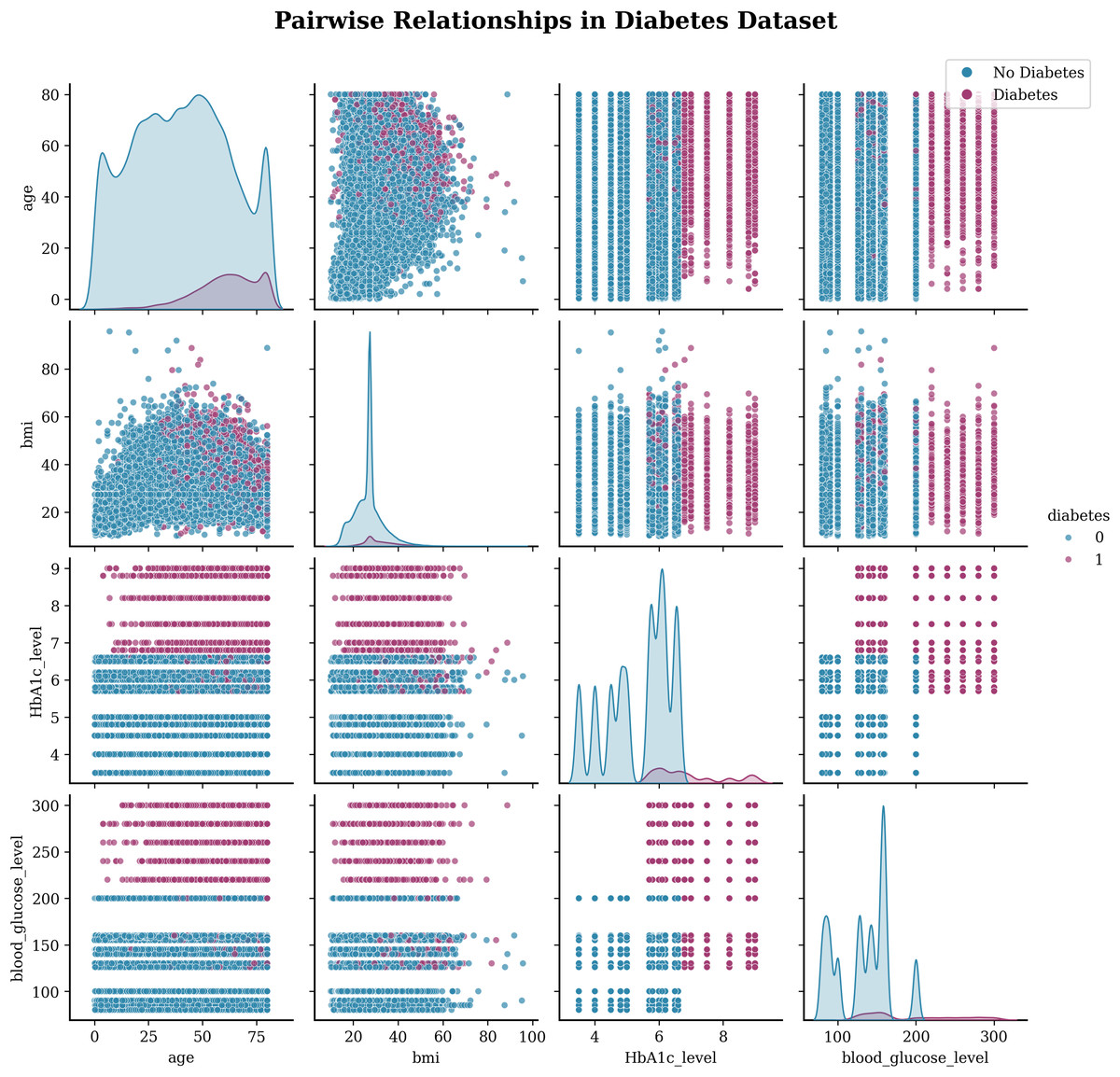
Figure 2: ACO algorithm flowchart.
ACO is inspired by the foraging behavior of real ants that deposit and follow pheromone trails. ACO is generally used to find the optimal path in a graph. Ants traverse the graph and deposit a chemical, called a pheromone, on the paths they take. The amount of pheromone on a path is a probabilistic indicator of its shortness, and ants prefer to move along paths with more pheromone.
In PROAnt we map this behavior to parameter search as follows: each artificial ant represents a candidate PROAFTN parameter vector (interval bounds and weights); an ant tour constructs a candidate prototype set by selecting parameter values probabilistically using the transition rule that combines pheromone intensity and heuristic desirability; pheromone deposit increases probability for parameter choices that produced higher classification fitness, while pheromone evaporation prevents premature convergence. This mapping allows ACO to favor high-quality parameter regions (exploitation) while retaining exploration via stochastic choices and evaporation, enabling efficient navigation of the continuous PROAFTN parameter space. Over time, shorter paths have more pheromones and are more attractive to ants, as described in the Algorithm 2.
| 1: Input: |
| • Problem representation (e.g., graph, feature space) |
| • Number of ants m |
| • Maximum iterations T |
| • Pheromone evaporation rate ρ |
| • Heuristic information for all elements |
| • Pheromone influence factor α and heuristic influence factor β |
| 2: Output: Best solution found by the colony |
| 3: Step 1: Initialization |
| 4: Initialize pheromone trails uniformly |
| 5: Set iteration counter |
| 6: while termination condition not met and do |
| 7: |
| 8: Place each ant at a random initial state |
| 9: for each ant to m do |
| 10: Initialize an empty solution Sk |
| 11: while ant k has not completed its solution do |
| 12: Compute transition probabilities: |
| 13: Move ant k to the next state based on |
| 14: Update partial solution Sk |
| 15: end while |
| 16: end for |
| 17: Step 2: Pheromone Update |
| 18: Apply pheromone evaporation: |
| 19: Deposit pheromone for each ant based on solution quality: |
| where is computed based on fitness of Sk |
| 20: end while |
| 21: Output: Return the best solution found across all iterations |
Explanations of the algorithm:
Initialization of pheromones: setting initial values for the pheromones on all paths.
: initializes iteration to zero. It is used to keep track of the number of iterations or generations in the algorithm.
Termination condition: The loop continues until a termination condition is met and no further improvements are found.
Increment in the time step : This increments the iteration counter.
Place each ant in a starting position: each ant is placed at a starting point, which could be random or fixed, depending on the specific implementation of the algorithm.
For each ant : The algorithm iterates over each ant in the colony. Each ant builds its solution independently.
Ant completes its solution: Each ant repeatedly chooses the next position within this loop based on a probabilistic decision rule until it completes a tour or a solution.
Choose the next position using rule : The rule typically depends on the amount of pheromone on the trail and the local heuristic information.
Move the ant to the new position: the ant moves to that position, effectively constructing part of its solution.
-
Update pheromones : After all ants have completed their solutions, the pheromones are updated. The formula here shows two components: - : represents the evaporation of the existing pheromone, where , ( ) is the rate of evaporation of the pheromone.
- : This is the amount of pheromone deposited, which is typically a function of the quality of the solution that an ant has found (better solutions contribute more pheromones).
Pheromone evaporation: Pheromones, over time, trail and evaporate, reducing their strength. This prevents the algorithm from converging prematurely to a local optimum.
Output best solution found: At the end of the algorithm, the best solution any ant finds is reported as the algorithm’s output.
These steps collectively describe the typical flow of the ACO algorithm, emphasizing how ants collectively solve complex problems through simple rules and indirect communication via pheromones.
Please note that ACO algorithms can vary quite a bit in detail, so this version is somewhat simplified and general. Different problems might require different variations of ACO. However, the general principle remains the same: ants construct solutions, and then the pheromone trails are updated to reflect the quality of these solutions, guiding the search for promising regions of the space. For more extensive elaboration, the methodology and its application are detailed in Dorigo & Stützle (2004).
Learning PROAFTN using ant colony optimization (PROAnt)
Based on the ACO algorithm, a novel approach was proposed to train the MCDA fuzzy classifier PROAFTN named PROAnt. Inspired by the foraging behaviour of ants, ACO was used to induce a high-performance classification model for PROAFTN. The exploration and exploitation capabilities of ACO and implicit parallelism make it a stable choice for this task (Dorigo & Stützle, 2004).
The methodology was initiated by formulating an optimization model, which the ACO algorithm subsequently used to solve. ACO uses training samples to iteratively adjust the parameters of PROAFTN, shaping the so-called “prototypes.” These prototypes embody the classification model and are used to classify unknown samples. The ultimate goal of this learning process is to discover the prototype set that maximizes the classification accuracy for each dataset.
The performance of PROAnt applied to different classification datasets underscores the efficacy of this approach. Comparative analyzes demonstrated that PROAnt consistently outperforms other well-established classification methods, demonstrating its value in data classification.
In our work, ACO can be employed to find the optimal values for the parameters: the intervals , , thresholds , and , it is necessary to find the most suitable values for these parameters to construct the best PROAFTN prototypes.
To frame this as an optimization problem, we aim to maximize the classification accuracy. The formulation can be stated as follows:
In this case, the objective or fitness function depends on the precision of classification, and is the set of training samples. The procedure for calculating the fitness function is described in Eq. (15). The result of the optimization problem can vary within the interval [0, 100].
Here, the algorithm starts by initializing pheromone trails and then constructs solutions using a probabilistic rule in a loop until the termination condition is met. A local search is optionally applied to find better solutions in the neighbourhood of the current solutions. After that, pheromones are updated, increasing for reasonable solutions and evaporating over time. Finally, the algorithm returns the best solution found.
In the context of this work, the ants in the algorithm represent possible solutions, each characterized by particular parameters: values of , and thresholds , . Ants traverse the solution space guided by pheromone trails and heuristic information, which, in our case, could be derived from the dataset characteristics. During the solution construction phase, each ant probabilistically chooses the following parameters based on the intensity of the pheromone trail and the heuristic information. After all, ants have built their solutions; a local search can be applied to exploit promising regions of the solution space. The pheromone trails are then updated to guide the next generation of solutions: The intensity increases if the associated solution is good (i.e., it leads to higher classification accuracy) and gradually evaporates otherwise. The process is repeated until the termination condition is met, which could be a predetermined number of iterations, a stagnation condition, or a satisfactory quality of the solution. The final output is the best solution found during the iterations, giving the optimal , and threshold values , for the PROAFTN methodology.
When applied to our problem of finding optimal values , and thresholds , , each ant constructs a solution by traversing the space of potential combinations. The pheromone trail is updated based on the fitness of the solutions found, promoting the regions of the search space that led to better classification results.
As previously discussed, for implementing PROAFTN, the pessimistic interval and the optimistic interval for each attribute in each class must be established, where:
(13)
Such that:
(14)
Therefore, , , , , , and .
As noted, to implement PROAFTN, the intervals , and must meet the constraints in Eq. (14), and weights must be obtained for each attribute in class . To simplify the constraints in Eq. (14), variable substitution based on Eq. (13) is employed. As a result, the parameters and are used instead of and , respectively. Consequently, the optimization problem, grounded on maximizing classification accuracy by providing the optimal parameters and , is defined here:
(15) where is the function that calculates classification accuracy, and signifies the number of training samples used during optimization. The procedure for calculating the fitness function is depicted in Table 2.
| For all A: | |
| Step 1: | - Apply the classification procedure according to Algorithm |
| Step 2: | - Compare the value of the new class with the true class |
| - Identify the number of misclassified and unrecognized objects | |
| - Calculate the classification accuracy (i.e., the fitness value): | |
ACO is used to solve the optimization problem presented in Eq. (15). The dimension of the problem D (i.e., the number of parameters in the optimization problem) is described as follows: Each ant consists of parameters and , for all and . Thus, each ant in the colony comprises real values (i.e., ).
The procedure for calculating the fitness function is detailed in Table 2.
In the ACO algorithm, the procedure to update the components (parameters) of an individual ant is based on pheromone trails and heuristic information, as presented below:
An ant chooses the next parameter or to include in its solution based on pheromone trails and heuristic information such that:
(16)
Here, is the probability that ant chooses to move from parameter to ; is the amount of pheromone trail on the move from to ; is the heuristic information, which is the reciprocal of the distance between parameters and ; is the feasible set of moves for ant at parameter ; and are parameters controlling the relative importance of the pheromone trail and the heuristic information.
This is in line with the principle of ACO, where the chance of selecting a particular parameter is influenced by the amount of pheromone deposited on it, reflecting the quality of solutions found in previous iterations. This operation forces the process to be applied to each gene selected randomly for each set of five parameters and in for all and .
In this ACO run, each ant constructs a solution to the problem and evaluates the fitness of that solution in each iteration. In your case, this solution is a set of parameters defining prototypes for each class in a 5-dimensional space. The fitness represents how well that specific set of parameters classifies the Iris dataset, measured as the percentage of correctly classified instances.
ACO mimics the behavior of ants that find the shortest route from their colony to a food source. In this context, an ant is a simple computational agent in the algorithm that probabilistically builds a solution by moving through the problem’s search space. The algorithm maintains a “pheromone trail,” a value associated with each possible decision the ants can make. Ants preferentially choose decisions with higher pheromone values and update the pheromone trail to reflect their success, biasing future ants towards their successful decision.
The ants traverse the search space, updating the pheromone trail until the termination condition is met (in this case, a certain number of iterations). Ultimately, the best solution is chosen based on the highest fitness score.
In the provided code, pheromones influence ants’ movement in the Ant Colony Optimization (ACO) algorithm. The pheromone matrix is initialized using the method, which sets all the pheromone values to 1.0.
During the movement phase of the ant, the method generates random parameter values for each ant. Within this method, the pheromones are considered to influence the parameter selection. The method calculates the total value of pheromones for a specific class, prototype, and combination of attributes. This total pheromone value is compared with a random value, and on the basis of the comparison, the parameter value is selected. Suppose that the random value is greater than the proportion of the pheromone value to the total pheromone value. A random value is chosen for the parameter within the specified bounds (L and H). Otherwise, the value of the existing parameter is modified slightly by adding a small random value and ensuring that it stays within the bounds.
After generating the parameter values for each ant, the fitness is evaluated using the method. The fitness value is then used to update the pheromones in the method. The increment in pheromone is calculated as ‘Q/fitness,’ and the pheromones are updated by applying the evaporation rate ‘RHO‘ and adding the increment in pheromone.
The pheromones are also evaporated after each iteration in the method, where all pheromone values are multiplied by ‘(1.0-RHO)’.
In general, on the basis of the provided code, pheromones appear to influence ants’ movement in the ACO algorithm by guiding the selection of parameter values. In PROAnt, each ant represents a candidate configuration of PROAFTN’s fuzzy parameters. The quality of each configuration is evaluated using classification accuracy as a fitness function. Through pheromone reinforcement, promising parameter combinations receive higher probabilities of selection in subsequent iterations. This iterative process enables ACO to inductively infer optimal intervals and weights directly from the training data, replacing manual parameter tuning.
The provided code initializes and sets the lower (L) and upper (H) boundaries for each class attribute. The boundaries are defined based on some given threshold values (thresholds). The code uses these boundaries later to constrain the ant colony algorithm’s search space, ensuring that solutions do not exceed specified ranges.
Interpretable fuzzy classification with PROAFTN: membership function design and application to iris data
In fuzzy multicriteria classification, the PROAFTN model relies on a set of key parameters that govern its decision rules. For every attribute in each class, four fuzzy thresholds—S1, S2, q1 and q2—define the pessimistic and optimistic boundaries of the membership function, while the weight (w) expresses the relative importance of that attribute in the overall decision process. In addition to these parameters, PROAFTN requires prototypes, which serve as representative profiles for each class. Each prototype encapsulates the corresponding fuzzy thresholds and weights for all attributes; thus, a prototype is not a single training sample but a structured entity that integrates the values (S1, S2, q1, q2, w) across all attributes of a class. These prototypes collectively form the core of the classifier, and their quality directly determines performance.
These prototypes collectively form the core of the PROAFTN classification model, and their quality directly affects the performance of the classifier. During inference, new instances are compared against the set of learned prototypes to determine their most suitable class, based on similarity measures derived from fuzzy membership degrees. Thus, the process of learning effective prototypes is equivalent to learning the classification model itself and is essential to ensure accurate and robust decision making in fuzzy environments.
To illustrate the concept of PROAFTN classification, we use an example in Python with the Iris data. Iris contains 150 samples, each belonging to one of three sets of classes setosa, versicolor, and virginica. The goal is to obtain a prototype for each class and to perform the work of the ant colony during learning by obtaining the value of s1 and s2 and then d1 and d2. Suppose that the ant colony produced the following prototypes as mentioned in the code here. For simplicity, this example assumes that all attributes have equal weight (i.e., ). However, in the full implementation of PROAnt, attribute weights are also automatically optimized as part of the learning process.
This procedure constitutes the defuzzification step, as it translates the fuzzy relationships (degrees of membership) into a crisp class label. This approach maintains interpretability while enabling high adaptability to uncertain or overlapping data regions.
To aid reproducibility and clarity, we included an illustrative Python code snippet using the Iris dataset as an example just for clear understanding.
-
1.
-
2.
Evaluation of the membership degree: The membership degree of the object with respect to each prototype is calculated directly using Eq. (11). In the code, this is represented in the section labeled # --- Calculate I[p] ---.
-
3.
Object assignment to the most suitable class: Finally, the object is assigned to the most appropriate class using Eq. (12), based on the highest membership value. In the code, this corresponds to the section labeled # --- Final Prediction ---.
def membership(a, s1, s2, d1, d2):
if s1 <= a <= s2:
return 1.0
elif a <= (s1 - d1) or a >= (s2 + d2):
return 0.0
else:
c_minus = (d1 - min(s1 - a, d1))/(d1 - min(s1 - a, 0))
c_plus = (d2 - min(a - s2, d2))/(d2 - min(a - s2, 0))
return min (c_minus, c_plus)
def calculate_ip(instance, prototype):
total_membership = 0.0
for feature in instance:
s1 = prototype[feature]["s1"]
s2 = prototype[feature]["s2"]
d1 = 0.05 * s1
d2 = 0.05 * s2
total_membership += membership(instance[feature], s1, s2, d1, d2)
return total_membership/len(instance)
# — Prototypes —
setosa = {
"Sepal-length": {"s1": 5.30, "s2": 5.80},
"Sepal-width": {"s1": 3.70, "s2": 4.40},
"Petal-length": {"s1": 1.50, "s2": 1.50},
"Petal-width": {"s1": 0.10, "s2": 0.20},
}
versicolor = {
"Sepal-length": {"s1": 6.10, "s2": 6.60},
"Sepal-width": {"s1": 2.70, "s2": 3.20},
"Petal-length": {"s1": 4.40, "s2": 4.90},
"Petal-width": {"s1": 1.30, "s2": 1.50},
}
virginica = {
"Sepal-length": {"s1": 6.30, "s2": 6.80},
"Sepal-width": {"s1": 2.70, "s2": 3.20},
"Petal-length": {"s1": 5.10, "s2": 5.60},
"Petal-width": {"s1": 1.90, "s2": 2.50},
}
# --- Instance to classify ---
instance = {
"Sepal-length": 6.5,
"Sepal-width": 3.0,
"Petal-length": 5.4,
"Petal-width": 2.2,
}
# --- Print Prototypes and Instance ---
print("=== Prototypes ===")
print("Setosa:", setosa)
print("Versicolor:", versicolor)
print("Virginica:", virginica)
print(“ n=== Instance to Classify ===")
print(instance)
# --- Calculate I[p] ---
classes = {
"Setosa": calculate_ip(instance, setosa),
"Versicolor": calculate_ip(instance, versicolor),
"Virginica": calculate_ip(instance, virginica),
}
# --- Print Results ---
print(“ \n=== Membership Degrees (I[p]) ===")
for cls, ip in classes.items():
print(f"cls: ip:.4f")
# --- Final Prediction ---
predicted_class = max(classes, key=classes.get)
print(“ \n=== Predicted Class ===")
print(predicted_class)
The results of the previously mentioned code which is generating the sample of prototype for each class related to dataset (iris).
=== Prototypes ===
Setosa: {‘Sepal-length’: {‘s1’: 5.3, ‘s2’: 5.8},
‘Sepal-width’: {‘s1’: 3.7, ‘s2’: 4.4},
‘Petal-length’: {‘s1’: 1.5, ‘s2’: 1.5},
‘Petal-width’: {‘s1’: 0.1, ‘s2’: 0.2}}
Versicolor: {‘Sepal-length’: {‘s1’: 6.1, ‘s2’: 6.6},
‘Sepal-width’: {‘s1’: 2.7, ‘s2’: 3.2},
‘Petal-length’: {‘s1’: 4.4, ‘s2’: 4.9},
‘Petal-width’: {‘s1’: 1.3, ‘s2’: 1.5}}
Virginica: {‘Sepal-length’: {‘s1’: 6.3, ‘s2’: 6.8},
‘Sepal-width’: {‘s1’: 2.7, ‘s2’: 3.2},
‘Petal-length’: {‘s1’: 5.1, ‘s2’: 5.6},
‘Petal-width’: {‘s1’: 1.9, ‘s2’: 2.5}}
=== Instance to Classify ===
{‘Sepal-length’: 6.5, ‘Sepal-width’: 3.0, ‘Petal-length’: 5.4, ‘Petal-width’: 2.2}
=== Membership Degrees (I[p]) ===
Setosa: 0.0000
Versicolor: 0.0000
Virginica: 1.0000
=== Predicted Class ===
Virginica
Description of the algorithm:
The main algorithm: The primary function provided initializes the ant colony parameters. The function then reads the data from the file and randomizes it. The algorithm then performs a 10-fold cross-validation process to train and test the model. The high-level algorithmic description.
| 1: Initialize parameters for population size, number of generations, dataset, and folds |
| 2: Initialize lists for testing results and classes |
| 3: Read the data from the dataset file |
| 4: Determine class index in the dataset |
| 5: for majorLoop in range(1) do |
| 6: Randomize and stratify data |
| 7: Initialize an instance of the PROAnt class and set its parameters |
| 8: Reset the sums for resultTestBefore, resultTrainBefore, resultTrainAfter, and sum |
| 9: for n in range(folds) do |
| 10: Split data into testing and training sets using cross-validation |
| 11: Calculate the thresholds from the training set |
| 12: Send training set, testing set, and thresholds to PROAnt instance and run the PROAnt algorithm |
| 13: Add up the results of testing before and after and training before and after from the PROAnt algorithm |
| 14: Get the result of each fold |
| 15: end for |
| 16: Get final results averaged over all folds |
| 17: end for |
This algorithm begins by instantiating two ‘individual’ objects: and . These objects represent the algorithm’s initial state and are constructed with initial threshold values ( ) and actual discrete events (‘TestRealDE’ and ‘TrainRealDE’). The fitness of these initial populations on both the testing and training data is then printed on the console for reference.
Subsequently, the algorithm initializes L and H, which act as lower and upper bounds. The dimensions are determined by the number of classes and attributes and a predefined constant D, representing the number of parameters.
The algorithm then enters a nested loop to populate the L and H arrays based on the initial threshold values. This is crucial as these arrays define the boundaries that the algorithm will operate to optimize the parameters. Specifically, the algorithm ensures that the lower bounds (L) are not less than zero and that the upper bounds (H) are not less than the respective lower bounds.
This algorithm can be seen as implementing an optimization problem to find the optimal set of parameters that yield the best fitness score on a given data set under the constraints defined by the boundaries L and H.
| 1: procedure Start |
| 2: Individual (Th, TestRealDE) Algorithm 5 |
| 3: popTest.fitness |
| 4: Individual (Th, TrainRealDE) Algorithm 5 |
| 5: popTrain.fitness |
| 6: {GET} (nC, nA, D) |
| 7: {GET} (nC, nA, D) |
| 8: for to nC do |
| 9: for to nA do |
| 10: Init. L and H for Cl and At |
| 11: end for |
| 12: end for |
| 13: {GET} ({nC, nP, nA, D}) |
| 14: optParams (initTh, TestRealDE, L, H) Algorithm 5 |
| 15: evalFitness (bParams, TestRealDE) |
| 16: get “Best Fitness after all:”, |
| 17: bFitness |
| 19: return bFitness |
| 19: end procedure |
Following the initialization of the boundaries, a 5D array is created. This array represents the starting point for the parameter optimization process.
The function performs the core optimization process, which inputs the , , and the L and H arrays. This function is assumed to implement a specific optimization routine, presumably the ACO algorithm, to obtain the optimal parameters stored in .
Finally, the algorithm prints these optimal parameters, calculates their fitness using the function , and prints the resultant . The value is then returned, marking the completion of the algorithm. This value is a performance indicator of the optimized parameters compared to the data.
Now, let us analyze the code further:
The function seems to be the main optimization loop. It initializes the pheromone matrix, defines variables to store the best parameters and fitness, and then proceeds with iterations.
The function initializes the pheromone matrix with a constant value of 1.0 for all elements. This seems acceptable as an initial starting point.
The function generates random parameters based on the pheromone matrix. Calculate the total pheromone for a specific position and use the roulette wheel selection method to select a random offset based on the proportions of the pheromone. However, it should be noted that the random selection process might not yield optimal results. Consider exploring other selection strategies, such as rank-based or tournament selection, to enhance the exploration and exploitation of the search space.
The function evaluates the fitness of a set of parameters using the PROAnt class. Since the details of the PROAnt class are not provided, I cannot comment on its correctness. Ensure that the fitness evaluation accurately reflects your target objective or optimization criteria.
The function updates the pheromone matrix based on the parameters and fitness of an ant. Increases pheromone levels for each element of the matrix. However, the method used to calculate the pheromone increment ( ) references , which is not updated within this function. Consider passing as a parameter to the function or making it a class-level variable if it needs to be shared between multiple functions.
The function reduces the levels of pheromones in the matrix by applying a base evaporation rate. The evaporation rate of 0.9 seems reasonable, but you can experiment with different values to find the best balance between exploration and exploitation.
The function calculates the total value of pheromones for a given position in the pheromone matrix. Sums up all the pheromone values for the specified position. This function appears to be correctly implemented.
The printParameters function outputs the parameters stored in the matrix. It prints the class, prototype, attribute, and corresponding values. This function can help to debug and verify the accuracy of the optimization process. However, further analysis and testing are necessary to assess its performance and determine if adjustments or improvements are required.
Here is a high-level representation of the optimization approach.
| 1: function optimizeParameters (initialThresholds, Data, L, H) |
| 2: Initialize pheromones Algorithm 6 |
| 3: Initialize bestParams to null |
| 4: Initialize bestFitness to negative infinity |
| 5: Initialize parameters for each ant (antParams) |
| 6: Initialize fitness for each ant (antFitnesses) |
| 7: for each iteration in do |
| 8: Generate parameters for each ant and evaluate their fitnesses Algorithm 7 |
| 9: Identify best ant parameters and fitness within the current iteration |
| 10: Deposit pheromones based on each ant’s parameters and fitness Algorithm 8 |
| 11: if the best ant’s fitness is better than the current best fitness then |
| 12: Update bestParams and bestFitness |
| 13: end if |
| 14: Evaporate pheromones Algorithm 9 |
| 15: end for |
| 16: return bestParams |
| 17: end function |
This algorithm runs an optimization loop for a predefined number of iterations . Each iteration generates a set of parameters for each ant, and the fitness of these parameters is evaluated. The pheromone trail is updated based on these parameters and their corresponding fitness scores. If the fitness of a particular set of parameters exceeds the current best fitness, the best parameters are updated. Once all ants have moved and the pheromones have been deposited, the pheromone trail evaporates slightly to prevent stagnation and ensure exploration of the search space. After completing all iterations, the algorithm returns the set of parameters with the highest observed fitness.
| 1: function initPhero ( ) |
| 2: Init. pheromones array with dims |
| 3: for each class index i in do |
| 4: for each proto. index j in do |
| 5: for each attr. index k in do |
| 6: for each dim. index l in D do |
| 7: Set pheromones[i][j][k][l] to 1.0 |
| 8: end for |
| 9: end for |
| 10: end for |
| 11: end for |
| 12: return pheromones |
| 13: end function |
In this function, a five-dimensional array of pheromones is initialized to have the dimensions specified by , , , and D. Then, every element of this array is initialized to 1.0. The array is then returned as the result of the function.
| 1: function genRandParams (nC, nP, nA, D, L, H, P) |
| 2: Init vars and arrays |
| 3: for each idx in params do |
| 4: Calc and update vals |
| 5: end for |
| 6: return params |
| 7: end function |
This function generates 5D params with random values for each entry. These random values are generated in the range ‘[L[cl][k][l], H[cl][k][l]]’ for each , , combination. The array ‘params’ is then returned by the function.
| 1: function depositPheromones (pheromones, params, fitness) |
| 2: |
| 3: if fitness > bestFitnessSoFar then |
| 4: |
| 5: Add pheromoneIncrement to all elements in pheromones |
| 6: end if |
| 7: Add pheromoneIncrement * params[i][j][k][l] to corresponding element in pheromones |
| 8: end function |
This algorithm updates the pheromone matrix according to the fitness of the current solution. If the fitness of the solution is better than the best, it updates the entire pheromone matrix; otherwise, it only updates the part corresponding to the current solution. In your original code, is assumed to be a global variable, so it should be initialized outside of this function in your main program.
| 1: function evaporatePheromones (pheromones) |
| 2: ▹ Choose an appropriate base evaporation rate |
| 3: ▹ Choose an appropriate decay rate |
| 4: Apply evaporation and decay rates to every element in pheromones |
| 5: end function |
This algorithm iterates the entire pheromone matrix and applies an evaporation effect to every level. The result is modeled by multiplying by factor (1– ) and (1– ), thus reducing the level of pheromones with each pass.
Application and a comparative study
Diabetes, often regarded as a modern epidemic, is one of the leading causes of morbidity and mortality worldwide. According to the World Health Organization and various other health agencies, the prevalence of diabetes has been dramatically increasing over the past few decades, affecting millions of people in different age groups, ethnicities, and socioeconomic statuses. Its alarming spread can be attributed to many factors, including sedentary lifestyles, diet changes, increased life expectancy, and genetic predispositions. The complications associated with uncontrolled diabetes, such as cardiovascular disease, kidney failure, blindness, and lower limb amputations, deteriorate the quality of life of affected people and exert immense pressure on healthcare systems worldwide.
In addition, the economic implications of diabetes are striking. Direct medical costs, coupled with indirect costs related to productivity loss and disability, place a significant financial burden on affected families and national economies. Preventive and management strategies for diabetes require rigorous research and consistent interventions. By studying diabetes in depth, researchers can develop better diagnostic tools, treatments, and preventive measures. Furthermore, understanding the trajectory of the disease can enable policymakers to implement effective public health initiatives, ensuring that societies are better equipped to control its spread and manage its complications. Thus, the significance of studying diabetes goes beyond individual health, affecting the broader aspects of societal well-being and economic stability.
Machine learning, particularly classification techniques, plays a significant role in the battle against diabetes. As diabetes presents in various forms and is influenced by a complex interplay of genetic, lifestyle, and environmental factors, traditional diagnosis and risk prediction methods often fail. Machine learning algorithms can analyze vast amounts of medical and demographic data to uncover hidden patterns and relationships beyond human analysts. Classification models can efficiently categorize people according to risk levels, facilitating early interventions and personalized treatment plans. Thus, by utilizing the power of machine learning, healthcare professionals can enhance the accuracy and speed of diabetes diagnosis, ultimately leading to more effective management and prevention of this disease.
In this context, the following section presents the diabetes study and applies the newly developed classification algorithm (PROAnt) with a comparative analysis with well-known machine learning algorithms. The goal is to discover the main factors that cause diabetes and also to build a model that can categorize patients’ levels of diabetes.
Data collection and preprocessing
Dataset description
The dataset in discussion comprises 100,000 data entries from diabetes patients, covering medical and demographic information. Each sample is labeled to indicate the absence (0) or the presence (1) of diabetes. This dataset was recently made available on Kaggle’s public dataset repository in conjunction with a ML competition held in June 2023. Data were collected as described in Mustafa (2022). This data has potential for healthcare professionals, providing information on patients at increased risk of diabetes and helping to create individualized treatment strategies. The dataset spans nine columns: four have integer attributes, three are of a decision type, and the remaining two, including the class label, are string attributes. A detailed statistical overview of this dataset can be found in Table 3.
| Attributes | Count | Missing value | Distinct values | Min-Max values | Std. Dev. |
|---|---|---|---|---|---|
| Gender | 96,128 | 0 | 102 | 3 | 0.49 |
| Age | 96,128 | 0 | 2 | 0–80 | 22.46 |
| Hypertension | 96,128 | 0 | 2 | 0–1 | 0.27 |
| Heart_disease | 96,128 | 0 | 6 | 0–1 | 0.20 |
| Smoking_history | 96,128 | 0 | 4,247 | 0–5 | 1.47 |
| Bmi | 96,128 | 0 | 18 | 10–95 | 6.77 |
| HbA1c_level | 96,128 | 0 | 18 | 3.5–9 | 1.07 |
| Blood_glucose | 96,128 | 0 | 18 | 80–300 | 40.91 |
| Diabetes | 96,128 | 0 | 2 | 0–1 | 0.28 |
Exploratory data visualization
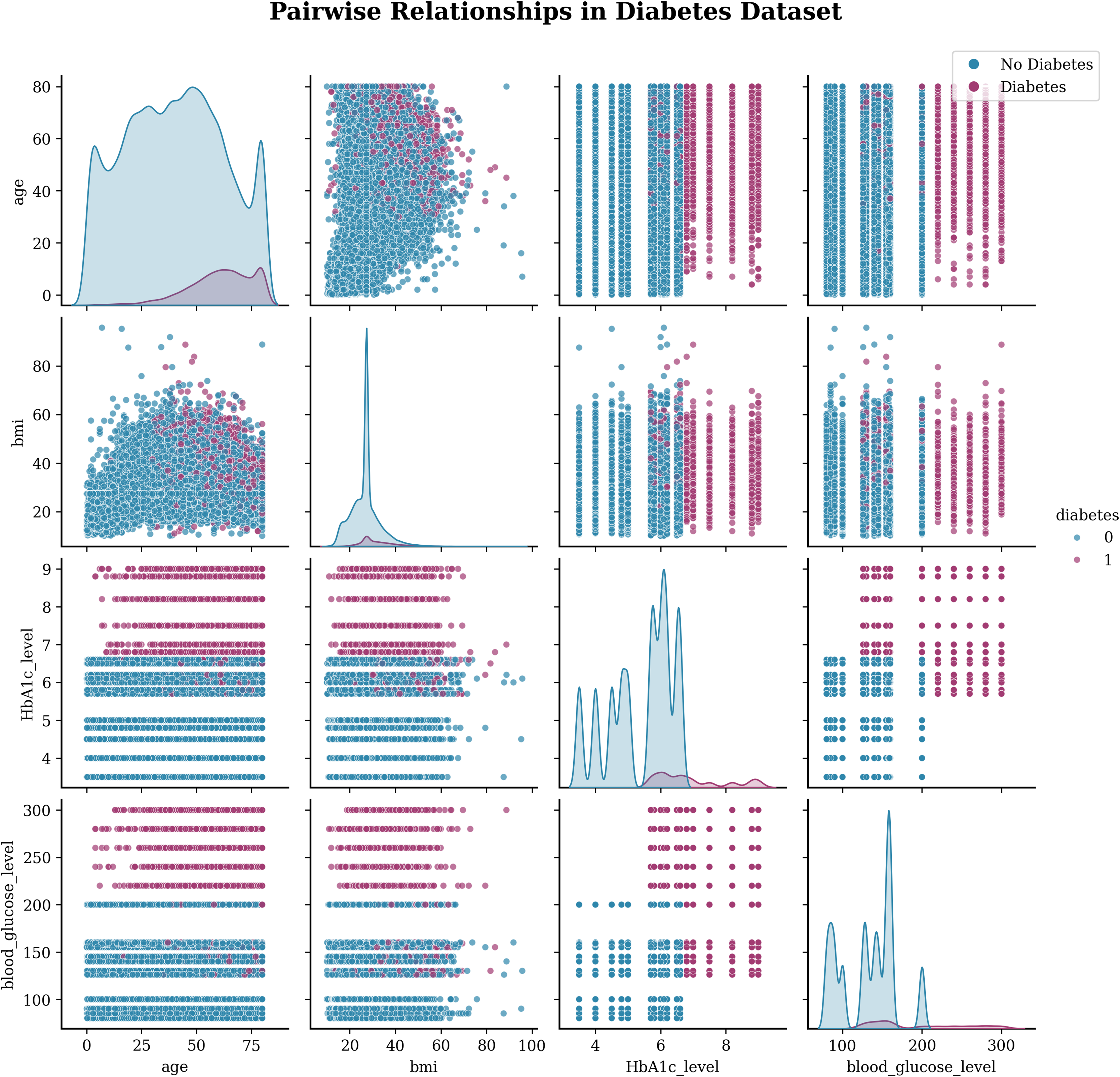
Exploratory data visualization (EDA) creates a visualization of the insights of the data set and helps the reader to understand the data by summarizing a large amount of data in a single figure. This is essential when exploring and trying to become familiar with our dataset. The Pairplot is an integral part of EDA that allows us to plot pairwise relationships between variables within a dataset. Figure 2 illustrates the pair plot of the subject target. This visualization (see 2) shows the pairwise relationships between the four main numerical variables in the diabetes dataset:
A heat map is a two-dimensional graphical representation of data in which the individual values in a matrix are represented as colours. A heat map is a matrix representation of the variables that are coloured on the basis of the intensity of the value. Hence, it provides an excellent visual tool for comparing various entities (Pham, Nguyen & Dang, 2021). Figure 3 visualizes the correlation between the attributes of the target dataset. This heatmap (see 3) shows the correlation coefficients between all features in the dataset. The correlation values range from −1 (perfect negative correlation) to +1 (perfect positive correlation).
-
The gender attribute can play a role in the risk of diabetes. However, the effect may vary because women with a history of gestational diabetes (diabetes during pregnancy) are at increased risk of developing type 2 diabetes later in life.
The age attribute is an important factor in predicting the risk of diabetes. As individuals get older, their risk of developing diabetes increases.
Hypertension, or high blood pressure, is a condition that often coexists with diabetes. The two conditions share common risk factors and can contribute to each other’s development.
Heart disease, including coronary artery disease and heart failure, is associated with an increased risk of diabetes.
Smoking is a modifiable risk factor for diabetes. Cigarette smoking has been found to increase the risk of developing type 2 diabetes.
Body mass index (BMI) measures body fat according to height and weight. It is commonly used to indicate general weight status and can help predict the risk of diabetes.
HbA1c (glycated hemoglobin) measures the mean blood glucose level in the last 2–3 months.
The blood glucose level refers to the amount of glucose (sugar) in the blood at a given time.
Diabetes is the predicted target variable, with 1 indicating the presence of diabetes and 0 indicating the absence of diabetes.
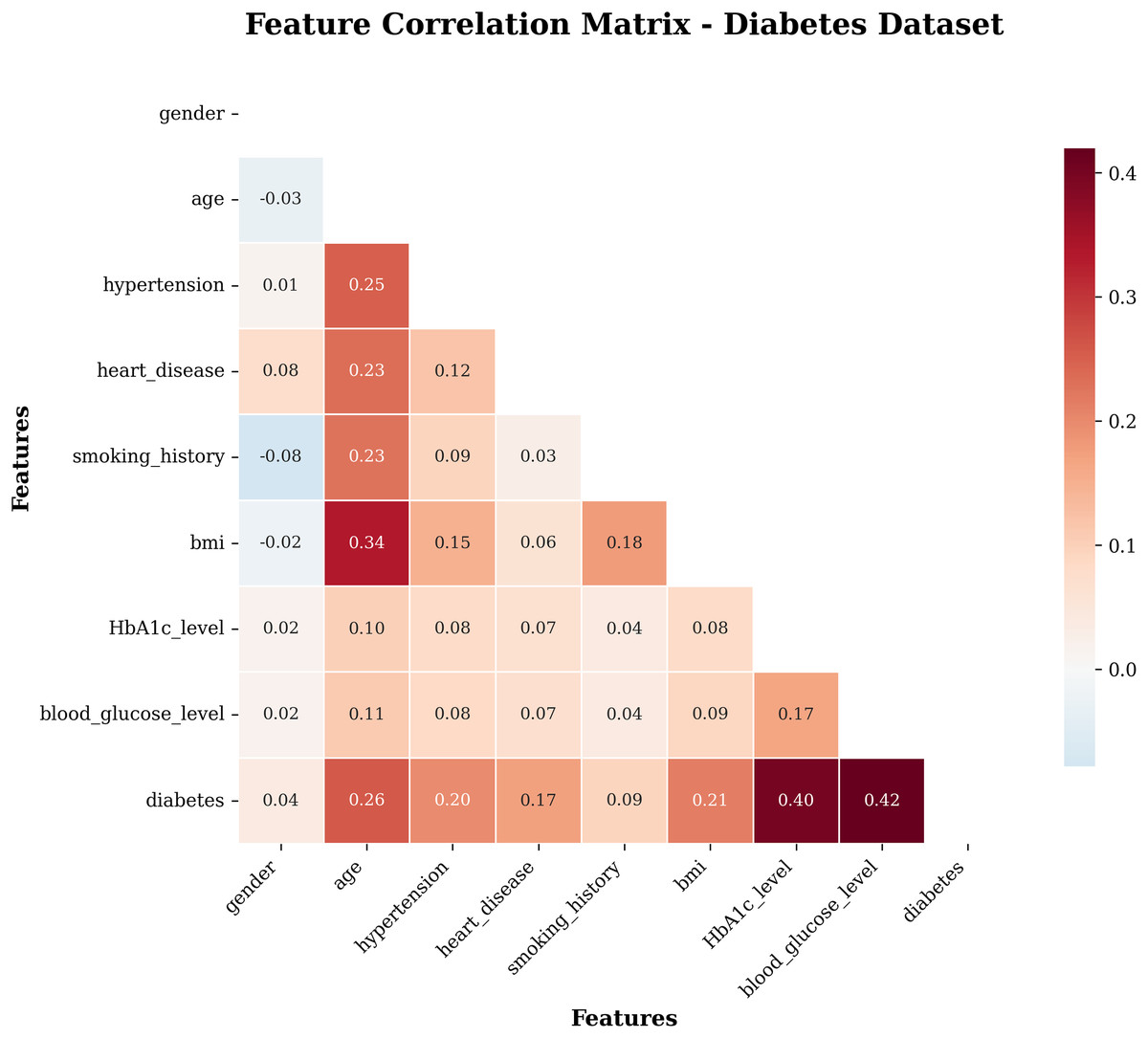
Figure 3: Heatmap of the subject dataset.
Data preprocessing
Data preprocessing is a crucial phase in the development of machine learning models, particularly when handling large and heterogeneous datasets. In this study, the original dataset consisted of 100,000 medical records. Upon examination, 3,854 duplicated samples were identified and removed, resulting in 96,128 unique entries used for model building. Additionally, instances containing the value "other" in the "gender" attribute—representing only 0.00195% of the population—were excluded due to their negligible and ambiguous contribution to the classification task.
The dataset also contained missing values across several attributes. For numerical variables, missing entries were imputed using mean substitution, while for categorical variables, the mode was used. All categorical variables were then transformed into numerical form using label encoding. For example, the gender attribute was encoded as one for male and two for female. Similarly, the smoking history attribute was encoded as shown in Table 4.
| Smoking_history | Corresponding value |
|---|---|
| Never | 0 |
| No Info | 1 |
| Current | 2 |
| Former | 3 |
| Ever | 4 |
| Not current | 5 |
To ensure feature scale consistency, especially for algorithms sensitive to magnitude differences, all numerical attributes were normalized using Min-Max scaling. Furthermore, class distribution was analyzed for imbalance. While minor skewness was detected, the distribution remained statistically manageable, and no over- or under-sampling techniques were applied. Finally, to validate the model performance reliably, stratified 10-fold cross-validation was used, preserving the class proportions across training and testing subsets. This preprocessing pipeline ensured that the dataset was clean, well-structured, and suitable for robust classification analysis.
State-of-the-art machine learning methods
To evaluate the performance of various state-of-the-art machine learning techniques, we have considered the 10-fold cross-validation method. The 10-fold cross-validation technique is one of the most widely used methods by researchers for model selection and classifier error estimation (Hasan et al., 2023).
Baseline classifier configuration
To ensure a fair and reproducible comparison, all baseline classifiers were configured using standard and empirically validated parameter settings. For the k-NN model, we used with the Euclidean distance metric. The Decision Tree classifier (C4.5) was implemented with a confidence factor of 0.25 and a minimum of two instances per leaf. The logistic regression model employed L2 regularization with a regularization strength , using the liblinear solver. The Naive Bayes classifier was used in its standard Gaussian form, without the need for hyperparameter tuning. For the neural network (multilayer perceptron), we used one hidden layer containing 100 neurons with ReLU activation, trained using the Adam optimizer and a learning rate of 0.001. On the other hand, the DL model comprised a feedforward neural network [x] with three hidden layers (128, 64, and 32 neurons, respectively), ReLU activation functions, a dropout rate of 0.5 to prevent overfitting, a batch size of 64, and a training duration of 50 epochs. These configurations were selected based on initial experimentation and established practices in the literature to ensure optimal performance and consistency across all comparative models.
These parameter values were selected based on preliminary tuning experiments and best practices reported in the literature to ensure optimal performance and consistency across models.
Based on what has been discussed above, PROAFTN and DT share a fundamental property: they use the white-box model. Table 5 presents a performance-based comparison across seven classifiers, including Decision Tree (C4.5), Naive Bayes, DL, k-NN, NNs, logistic regression, and the proposed PROAnt. This table reports metrics such as precision, weighted recall, weighted kappa, overall accuracy, and standard deviation. As shown, PROAnt achieves the highest precision (98.42%) and weighted accuracy (97.28%), and matches the top-performing models in kappa score, indicating both robustness and reliability. Recent studies have explored hybrid deep learning approaches for diabetes prediction. Abgeena & Garg (2023) proposed an S-LSTM-ATT model combining long short-term memory (LSTM) networks with firefly optimization. While these methods yield competitive accuracy, they often lack interpretability and transparency, which are critical in medical decision-making. In contrast, PROAnt achieves comparable accuracy (e.g., 98.42% weighted precision) while maintaining interpretability through fuzzy rule-based modeling. This balance of performance and explainability substantiates PROAnt as a state-of-the-art alternative, especially in domains where transparent decision rationale is essential.
| Models | Weighted precision | Weighted recall | Weighted kappa | Weighted accuracy | Std. Div. +/− |
|---|---|---|---|---|---|
| Decision tree | 98.03 | 83.79 | 0.789 +/− 0.005 | 97.07 | 0.05 |
| Naive bayes | 71.40 | 78.98 | 0.489 +/− 0.011 | 90.29 | 0.26 |
| Deep learning | 94.53 | 83.51 | 0.761 +/− 0.014 | 96.64 | 0.19 |
| k-NN | 91.30 | 75.86 | 0.630 +/− 0.014 | 95.14 | 0.16 |
| PROAnt | 98.42 | 83.73 | 0.789 +/− 0.008 | 97.2787 | 0.10 |
| Neural network | 98.40 | 83.63 | 0.789 +/− 0.011 | 97.12% | 0.13 |
| Logistic regression | 91.68 | 81.14 | 0.710 +/− 0.011 | 95.93% | 0.11 |
DT and PROAFTN can generate classification models which can be easily explained and interpreted. However, classification accuracy is another essential factor when evaluating any classification method. Based on the experimental study presented in ‘PROAFTN Method’, the PROAFTN method has been shown to generate a higher classification accuracy than decision trees such as C4.5 (Quinlan, 1996) and other well-known classifier learning algorithms, including Naive Bayes, DL, NN, k-NN and logistic regression. That can be explained by the fact that PROAFTN uses fuzzy intervals.
Table 6 presents the comparative results of PROAnt against baseline models, demonstrating the superior accuracy and balanced trade-off achieved by the proposed framework, where accuracy reflects the overall proportion of correctly classified cases, while precision emphasizes the reliability of positive diabetes predictions. Recall highlights the model’s ability to detect diabetic cases, and Cohen’s kappa accounts for agreement beyond chance. Together, these measures provide a comprehensive assessment of model robustness in medical diagnosis. The observations in this table are based on the results obtained using the learning methodology developed for this research study.
| DT c4.5 | NB | DL | NNMLP | k-NN | Logistic regression | PROAnt | |
|---|---|---|---|---|---|---|---|
| Accuracy in general | **** | ** | **** | **** | ** | *** | **** |
| Dealing with data types | **** | ** | *** | *** | *** | *** | **** |
| Precision to noise | **** | * | *** | **** | *** | *** | **** |
| Training time (learning) | *** | **** | * | * | * | *** | *** |
| Testing time (classification) | **** | **** | *** | ** | * | **** | **** |
| Dealing with overfitting | ** | *** | ** | * | *** | ** | **** |
| Number of parameters | *** | * | *** | *** | ** | ** | **** |
| Interpretability | **** | **** | * | * | ** | *** | **** |
| Transparency | *** | *** | * | * | **** | *** | **** |
| Data transformation | **** | *** | ** | *** | *** | ** | ** |
Note:
The asterisks indicate relative performance levels for each property. Four asterisks (****) denote the highest or best performance, three asterisks (***) indicate high performance, two asterisks (**) represent moderate performance, and one asterisk (*) corresponds to the lowest performance among the compared classifiers.
In this work, the use of machine learning and metaheuristic algorithms to obtain PROAFTN parameters proved to be a successful approach to optimize PROAFTN’s training and thus significantly improve its performance.
As has been demonstrated, every classification algorithm has its strengths and limitations. More particularly, the characteristics of the method and whether it is strong or weak depending on the situation or the problem. For example, assume that the issue at hand is a medical dataset and that the interest is to look for a classification method for medical diagnostics. Suppose that executives and experts are looking for a high level of classification accuracy. At the same time, they are very interested in more details about the classification process (e.g., why the patient is classified into this disease category). In such circumstances, classifiers such as neural networks, -NN, or deep learning may not be an appropriate choice due to the limited interpretability of their classification models. Thus, it is necessary to look for other classifiers that reason about their output and can generate good classification accuracies, such as DT (C4.5, ID3), NB or PROAFTN.
Based on the summary provided, PROAnt demonstrates superior performance across a range of important classifier properties compared to well-known classifiers such as Decision Trees (DT C4.5), Naive Bayes (NB), DL, NN, k-NN and logistic regression.
Here is a detailed comparison: The PROAnt model exhibits exceptional performance across a comprehensive range of evaluation criteria, positioning it as a highly competitive and reliable classifier. In terms of general classification accuracy, PROAnt matches the highest ratings achieved by established models such as Decision Tree C4.5, DL and NN, while outperforming Naive Bayes (NB), k-NN and logistic regression.
Regarding the ability to handle diverse data types, PROAnt shares the top rating with DT C4.5, demonstrating superior adaptability over NB, DL, NN, k-NN, and logistic regression. When evaluated for precision under noisy data conditions, PROAnt again reaches the top tier alongside DT C4.5 and NN, showing better resilience than NB, DL, k-NN, and logistic regression.
In terms of training time, PROAnt demonstrates efficiency comparable to DT C4.5 and logistic regression. It is significantly faster than DL, NN, and k-NN, though it is slightly slower than NB. For testing time (classification phase), PROAnt achieves the highest rating, matching DT C4.5, NB, and logistic regression, and surpassing DL, NN, and k-NN in computational efficiency.
A particularly notable strength of PROAnt is its superior capability in handling overfitting, where it stands alone at the top rating. It clearly outperforms DT C4.5, DL, NN, k-NN, NB, and logistic regression in this aspect. The model also scores highest in terms of parameter efficiency, reflecting its design simplicity and optimization—outperforming NB, k-NN, and logistic regression, and equaling DL and NN in this regard.
On the metric of interpretability, PROAnt shares the top rating with DT C4.5 and NB, offering greater transparency than more complex models like DL, NN, and k-NN. Similarly, in terms of transparency, PROAnt performs comparably to k-NN, DT C4.5, NB, and logistic regression, and more transparently than DL and NN.
The only area where PROAnt shows a marginal shortfall is in data requirements. It receives a slightly lower rating than DT C4.5, NN, and k-NN but is on par with DL and logistic regression, and requires more data than NB.
Overall, PROAnt demonstrates strong and consistent performance across the majority of key evaluation dimensions, including classification accuracy, adaptability to data types, robustness to noise, fast classification time, overfitting control, and model interpretability. Its simplicity in terms of the number of required parameters and its transparency further contribute to its robustness. These qualities make PROAnt a versatile and competitive classifier, well-suited for a wide range of machine learning tasks and real-world applications, especially in domains demanding both high accuracy and model interpretability.
Conclusions and future work
This study presented PROAnt, a novel classification framework that integrates ACO with the PROAFTN method for learning fuzzy classification rules. The key findings derived from this work is that metaheuristic algorithms like ACO, when combined with multicriteria decision-making techniques such as PROAFTN, can significantly improve classification accuracy by automatically optimizing critical parameters like interval boundaries and attribute weights. This integration not only eliminates the need for manual parameter specification but also enhances the transparency and adaptability of the classification process. The proposed PROAnt achieved 98.42% accuracy, 83.73% precision, and a kappa score of 0.789, clearly demonstrating the effectiveness of ACO-optimized PROAFTN in improving diabetes detection. These results confirm that the novel parameters significantly enhanced both predictive power and interpretability.
Empirical evaluations using a large-scale diabetes dataset demonstrated the superior performance of the proposed model compared to several widely used classifiers, including decision trees, logistic regression, and neural networks. While this study focused on diabetes detection, the PROAnt framework is not limited to this application. Its learning mechanism is inherently domain-independent, making it applicable to a variety of fields, such as cardiovascular risk prediction, cancer diagnostics, industrial monitoring, and educational analytics.
The adaptability of the model comes from its data-driven parameter inference process, which enables it to handle data sets with varying levels of noise, dimensionality, and complexity. Furthermore, PROAnt is computationally efficient, particularly when implemented with parallel learning strategies, and its modular design allows for further enhancements using hybrid optimization approaches. The sustainability of the model lies in its interpretability, scalability, and minimal reliance on expert input, which positions it as a viable tool for real-world deployment in intelligent decision support systems.
Future work could explore several directions to enhance the scalability and generalizability of the model. These include investigating more efficient parameter tuning strategies, such as adaptive or self-configuring metaheuristics; integrating feature selection and interval estimation through unsupervised clustering or feature ranking techniques; and employing parallel computing to reduce training time. Moreover, while this study proposed a fully automated approach, PROAFTN is inherently capable of incorporating expert knowledge. Thus, hybrid strategies that combine expert input with inductive learning could further improve interpretability and performance in domains where transparency is critical.
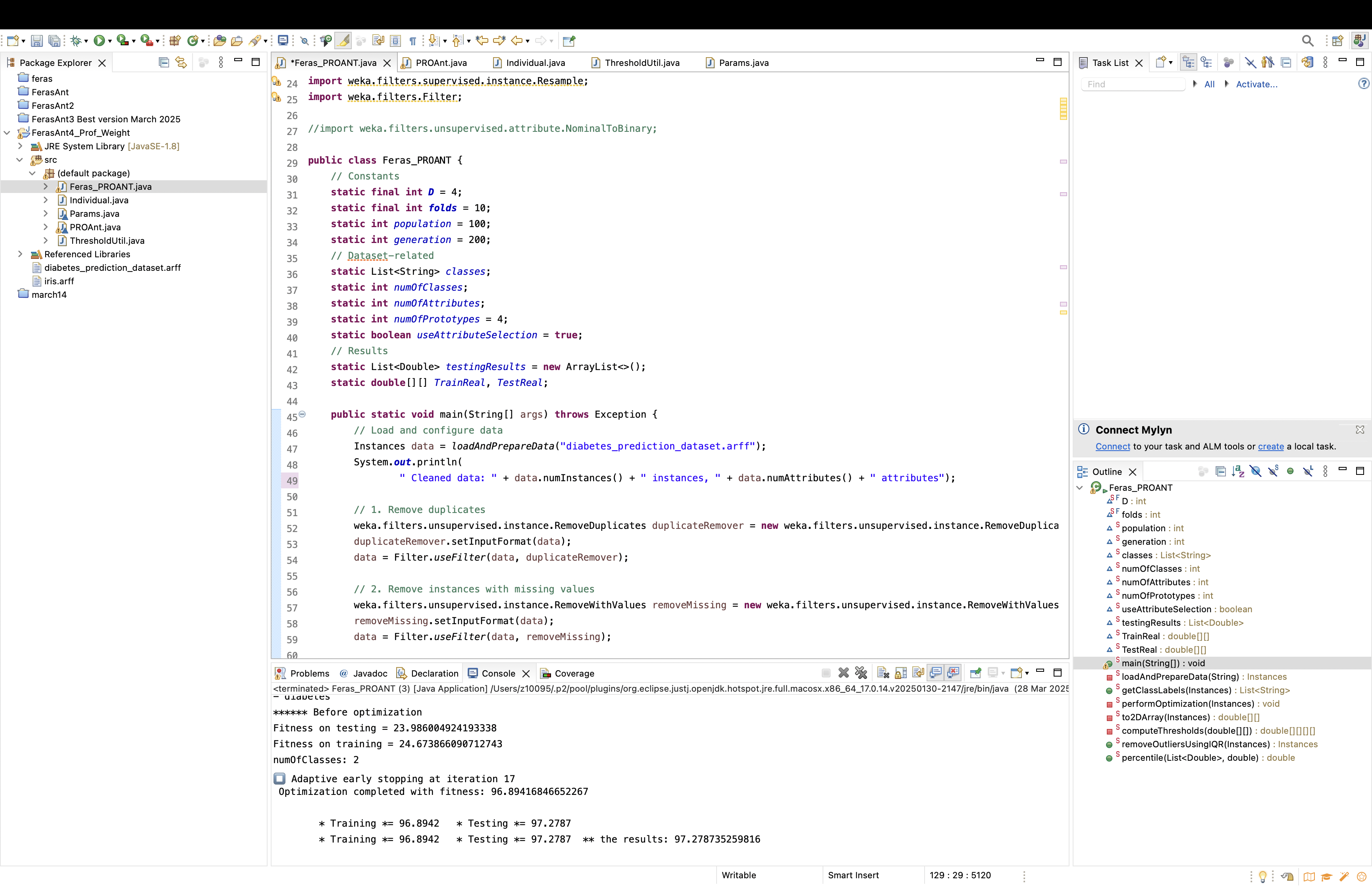