
Cursive character prediction using a deep learning model
- Published
- Accepted
- Received
- Academic Editor
- Davide Chicco
- Subject Areas
- Algorithms and Analysis of Algorithms, Artificial Intelligence, Computer Vision, Mobile and Ubiquitous Computing, Natural Language and Speech
- Keywords
- Convolutional neural network, Cursive character, Deep learning, Image preprocessing
- Copyright
- © 2025 Lee et al.
- Licence
- This is an open access article distributed under the terms of the Creative Commons Attribution License, which permits unrestricted use, distribution, reproduction and adaptation in any medium and for any purpose provided that it is properly attributed. For attribution, the original author(s), title, publication source (PeerJ Computer Science) and either DOI or URL of the article must be cited.
- Cite this article
- 2025. Cursive character prediction using a deep learning model. PeerJ Computer Science 11:e3332 https://doi.org/10.7717/peerj-cs.3332
Abstract
Cursive character (CC) recognition faces challenges owing to multifarious CC writing styles and complex character structures. Therefore, a universal CC identification system is essential. This study focuses on Chinese cursive characters and proposes a novel deep learning-based CC prediction model, along with a corresponding mobile application for real-time character recognition. The proposed model comprises three primary steps: data collection (from historical manuscripts, cleaned to remove noise); image preprocessing (including normalization, resizing, and augmentation); and prediction (involving hyperparameter optimization, regularization, and prediction using deep learning models). Transfer learning from convolutional neural networks such as Residual neural network (ResNet), Densely Connected Convolutional Networks (DenseNet), very deep convolutional network (Visual Geometry Group, VGG), and EfficientNet is employed. The model was trained and evaluated on a curated dataset of 99,296 images across 331 character classes, derived from Wang Xizhi’s ‘Grass Jue Song and Cursive Thousand Characters’. Using DenseNet-201, the proposed model achieved superior performance, with accuracy, precision, recall, and F1-score of 0.92, 0.92, 0.93, and 0.92, respectively. In contrast to existing work, which often focuses on smaller datasets or different scripts, this study introduces a large-scale recognition framework tailored for complex and visually similar Chinese cursive characters and demonstrates its practical deployment through a mobile application.
Introduction
Cursive penmanship is a form of writing in which the characters, called cursive characters (CCs), are written in a joined and flowing manner, which generally makes writing faster than with block characters. Many types of CCs exist, such as English, kanji, Japanese, Korean, and Urdu. In the case of Korean CCs, historical documents give us a glimpse into the past and provide valuable resources for exploring the culture, traditions, and general lifestyles of the Korean dynasty (Jalali, Kavuri & Lee, 2021). As a result, studies conducted in this area have provided information about cultural heritage and historical and linguistic backgrounds and helped interpret the historical writing of the manuscript (Jalali & Lee, 2020). However, these studies have faced challenges due to a lack of uniformity in writing styles and complex CC structures. Consequently, identifying CCs has become challenging for people who are unfamiliar with the format and a dearth of datasets to perform experiments. In addition, CCs are simple, many are very similar, and each person has intrinsic handwriting. Therefore, extensive reading experience is typically required to be able to decipher CC.
Considering the complexity of the task at hand and the limited number of prior studies, existing CC recognition models often focus on specific scripts or small datasets and rarely support real-time deployment. Moreover, generalization across cursive styles remains a major challenge, particularly for complex scripts such as Chinese cursive. To address these issues, we propose a deep learning-based system capable of recognizing Chinese cursive characters and delivering predictions via a real-time mobile application.
The model underlying our system is based on convolutional neural networks (CNNs), which have recently regained attention due to their ability to extract high-level features directly from raw input data (Zhao et al., 2024; Azimi et al., 2018). Over the past decade, CNNs have demonstrated excellent performance in various image-related domain, including classification, segmentation, and medical imaging (Zhang, Cui & Zhu, 2020; Kamilaris & Prenafeta-Boldú, 2018; Chen et al., 2021; Basu et al., 2022). These architectures provide high learning capacity, enhanced performance, and improved generalization (Kamilaris & Prenafeta-Boldú, 2018), especially with advances in computational hardware (Chen et al., 2021). CNNs are therefore well-suited to capture the subtle structural variations in cursive characters, particularly in historical scripts.
This study was conducted to develop a mobile-based system that predicts Chinese CCs with high accuracy. The user provides a CC image, which is pre-processed on the server, and the prediction result is returned to the application. The dataset used for training included 99,296 images across 331 character classes, derived from historical texts. To address data imbalance and improve model generalization, image augmentation techniques were applied during preprocessing (Goswami & Singh, 2024). The proposed model was evaluated against conventional CNN architectures using standard metrics such as accuracy, precision, F1-score, and recall. Experimental results confirm that our model outperforms other approaches.
The present study makes the following contributions:
Proposes a deep learning-based model for Chinese cursive character (CC) prediction, leveraging transfer learning from CNN-based architectures.
Demonstrates strong predictive performance of the proposed model, achieving 92% accuracy, 92% precision, 93% recall, and 92% F1-score.
Implements a real-time mobile application for CC recognition, integrating server-side preprocessing and prediction to support user-friendly interaction via smartphone input.
Constructs and publicly releases a large-scale dataset of 99,296 cleaned and preprocessed Chinese cursive character images derived from Wang Xizhi’s ‘Grass Jue Song and Cursive Thousand Characters’ to support transparency, reproducibility, and further research.
Related works
Table 1 summarizes related character recognition studies by author, approach, network, dataset, and dataset description. Chandio, Asikuzzaman & Pickering (2020) presented a convolutional feature fusion method with multiscale feature aggregation and multilevel feature fusion networks for Urdu character recognition in natural scenes. The multiscale feature aggregation network integrates the low- and mid-level convolutional features of different layers through up-sampling (Kopf et al., 2007) and element-by-element addition operations. Aggregation features are provided in a multilevel feature convergence network to be combined with high-level features. Finally, the aggregation and multilevel features are fused and passed to a SoftMax classifier to generate predictions. The network performance of Basu et al. (2022) was evaluated on three datasets: Chars74K, ICDAR03 (Antonacopoulos, Gatos & Karatzas, 2003), and a custom-developed Urdu character image dataset consisting of 18,500 manually segmented character images. Stochastic gradient descent (SGD) (Loshchilov & Hutter, 2017) optimization and sparse categorical cross-entropy loss function were used. The learning rate was optimized at 0.005, and the number of epochs for training was set to 80.
| Author | Network | Dataset | Dataset description |
|---|---|---|---|
| Chandio, Asikuzzaman & Pickering (2020) | Baseline + MSFA + MLFF Network | Chars74K, ICDAR03 | Urdu and English characters. |
| Clanuwat et al. (2018) | U-net | Kuzushiji | Contains Japanese characters. |
| Shi, Bai & Belongie (2017) | VGG-16 | SynthText, ICDAR2015, MSRA-TD500, ICDAR2013 | Consists of Chinese cursive characters. |
| Qin et al. (2020) | VGG-16 | ICDAR2015 | Includes Chinese cursive characters. |
| Hong & Kim (2020) | DenseNet-201 | Caoshu | Contains Chinese cursive characters. |
Clanuwat, Lamb & Kitamoto (2019) proposed KuroNet, a pre-modern Japanese text recognition model, and verified it experimentally. KuroNet rescales the given image to a standardized size of 640 × 640 pixels and uses the residual FusionNet of the U-Net architecture (Ronneberger, Fischer & Brox, 2015). The Japanese dataset used to train and evaluate KuroNet was created by the National Institute of Japan Literature (NIJL) (Clanuwat et al., 2018) and released in 2016. It consists of bounding boxes for all character positions in the text in pixel coordinates. Clanuwat et al. (2018) trained the model for 80 epochs and used the adaptive moment estimation (Adam) optimizer (Soydaner, 2020) with a learning rate of 0.0001, β1 of 0.9, and β2 of 0.999.
Shi, Bai & Belongie (2017) presented Segment Linking (SegLink) as a novel text detection method implemented as a simple and efficient CNN model. SegLink uses a pretrained VGG-16 network as its backbone. Six convolution layers detect segments and links, thereby providing high-quality deep features with granularity. SegLink was evaluated using augmentation with each standard evaluation protocol on three open datasets: ICDAR 2013 (Karatzas et al., 2013) Incidental Text, MSRA-TD500, and ICDAR 2015 (Karatzas et al., 2015). SegLink was optimized using the SGD algorithm with a momentum of 0.9. In 5–10 K iterations, the decay was fixed at 1e−3 and separately selected from other datasets through grid search in the holdout validation set.
Qin et al. (2020) presented a Chinese cursive dataset and combined ancient Chinese culture and artificial intelligence technology to improve the performance of the SegLink method. The process improved the feature extraction ability from image text by using squeeze and excitation operations. The importance of each feature channel is automatically acquired through learning. According to the importance of the feature channel, which achieves adaptive correction of the feature channel and improves the feature extraction ability of the backbone, valuable features are enhanced, and useless features are suppressed. All the proposed cursive datasets were written by Chinese cursive writers, and the images were annotated. The training and test set ratio was set to 4:1. The learning rate was set to 1e−3, the initial number of iterations was 60 k, which was followed by 30 k iterations.
Hong & Kim (2020) proposed an optimized DenseNet-201-based Caoshu character recognition model. Image resizing, binarization, and augmentation were performed as performance optimization techniques. The cross-entropy loss function was used to optimize the model, and SGD was set to a learning rate of 0.1 and a momentum of 0.9. The learning rate was set to drop by 0.1 every 30 steps. The Caoshu dataset used consisted of 527 classes from a possible 38,878 classes, and the original size of each image was adjusted to 224 × 224.
Materials and Methods
In this study, we propose a novel CC prediction model that contributes significantly to CC prediction by solving the data imbalance issue and enhancing the prediction accuracy. The proposed CC prediction model is illustrated in Fig. 1. It consists of three primary steps: data collection, image preprocessing, and prediction. In the data collection step, data collection and cleaning are carried out. Preprocessing is vital because it converts raw data into a well-organized form by processes such as noise reduction and quality enhancement to make the data suitable for prediction model algorithms. Finally, the prediction model uses CNN algorithms to learn from the training data and successfully predict the given input CC.
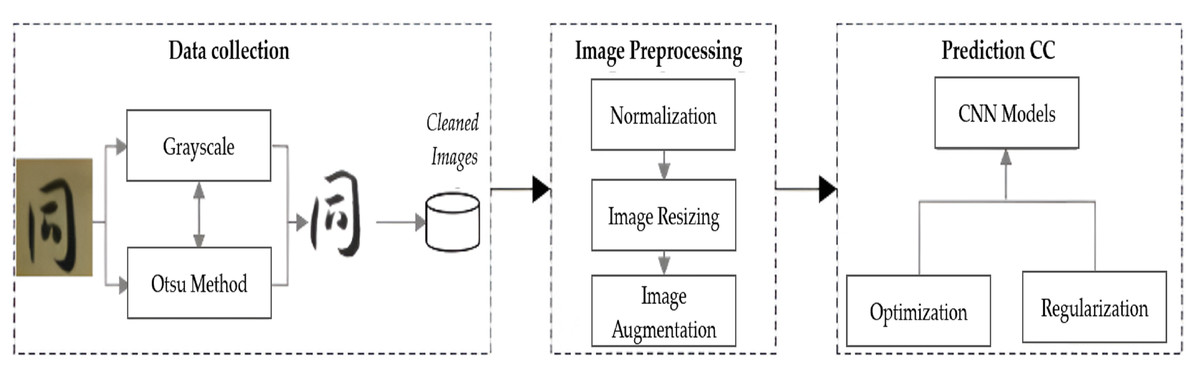
Figure 1: Flow of the proposed cursive characters prediction method.
Data collection
The dataset used in this study was created using images from Wang Xizhi’s ‘Grass Jue Song and Cursive Thousand Characters’. These two documents are used as baseline documents for CC learners. They contain a total of 1,549 characters (549 and 1,000 characters, respectively), but only 527 of the 1,549 available characters were used in this study. Each CC was converted into an image to construct our dataset.
The performance of most models is considerably affected by class imbalance. Therefore, we removed character classes with fewer than five available images, as such small sample sizes were found to contribute to unstable learning and poor generalization. After this filtering step, the final dataset contained 331 characters.
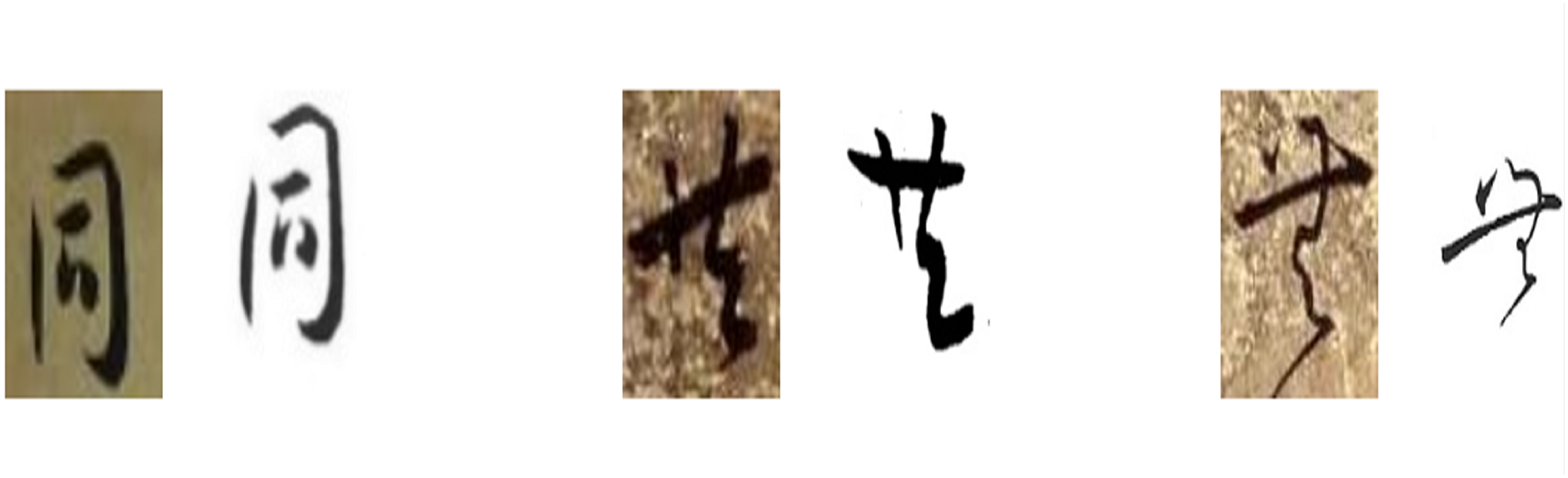
Each CC was obtained at a spatial resolution of 224 × 224 pixels and stored in the JPG file format, resulting in a dataset comprising 99,296 images. The CCs contained impurities that had to be cleaned for further processing; thus, image cleaning is a crucial task during preprocessing. The cleaning process reduces the number of noise signals in image pixels to a minimum by determining and removing a maximal amount of noise from the pixel with the signal from a shower and generating accurate information from the original data discarded of impurity for further processing (Shayduk, 2013). During the image cleaning process, red, blue, green (RGB) to grayscale conversion was performed on the CCs (Ojala, Pietikainen & Maenpaa, 2002). A grayscale image has only one dimension, whereas an RGB image is composed of three dimensions. This difference in dimensionality implies reduced computational requirements and simplification of preprocessing and prediction algorithms given the large amount of data that the RGB format may contain that is not required by the CC prediction model. After conversion to grayscale, Otsu’s method (Liu & Yu, 2009) was applied to remove the background other than the CC. Using thresholding, Otsu’s method divides the image values into two classes: panorama and background. Figure 2 shows samples of the cleaned CC images used, which are completely different from the original data, as can be seen.
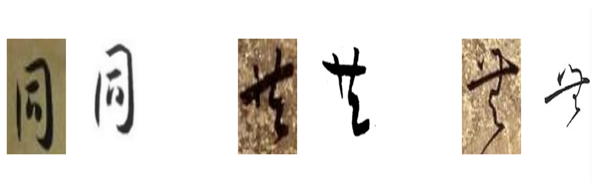
Figure 2: Sample original cursive characters (CCs) and their cleaned versions.
Image preprocessing
The prediction model step requires well-processed and organized data for further processing. Therefore, image preprocessing is crucial in our proposed model. Using the cleaned version of the original image data, the preprocessing step comprises normalization, image resizing, and image augmentation (Shorten & Khoshgoftaar, 2019). Normalization involves converting the normal numeric column value in the dataset to a standard scale [0–1], usually [0–255]. The normalization formula is defined in Eq. (1):
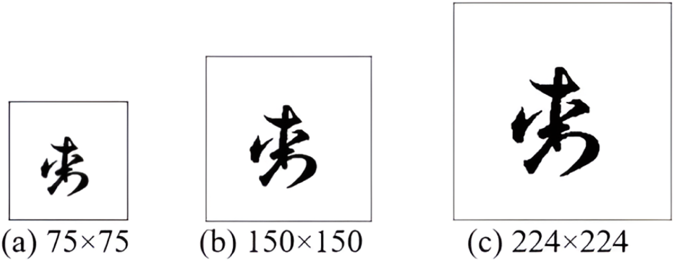
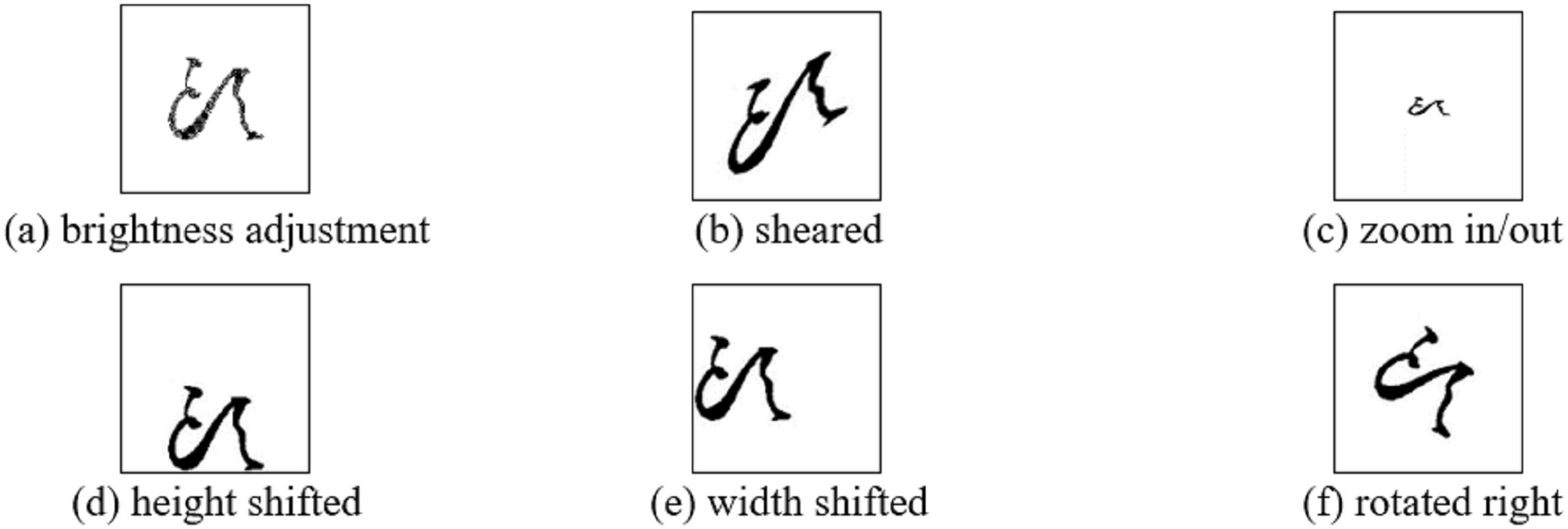
(1) where and represent the maximum and minimum values found in the images, respectively. Subsequently, image resizing is used to appropriately adjust the size of the images. Owing to the performance instability related to the difference in image sizes observed, for stable performance, the image is resized to a standard size and the 224 × 224 format was selected, as shown in Fig. 3. Finally, image augmentation is performed owing to the limited training datasets required for the CNN operations. Figure 4 presents six geometric transformation image techniques: brightness, shear, zoom, height shift, width shift, and rotation. These augmentation techniques were applied at factors of 0.01, 0.1, 0.2, 0.1, 0.1, and 10, respectively.
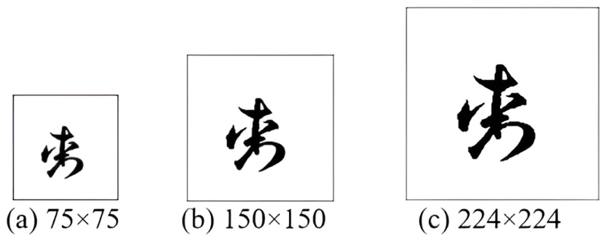
Figure 3: (A–C) Resizing an actual image.
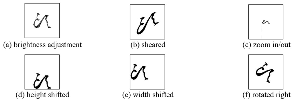
Figure 4: (A–F) Result of six data augmentation techniques applied to an original CC image.
Prediction model
The proposed prediction model takes an input image containing a CC and interprets the picture to predict the CC class in the given image. After proper cleaning and preprocessing, a sufficient number of images were noise-free for training, validation, and testing purposes. We conducted experiments using the proposed model with the transfer learning approach from various CNN algorithms, including the very deep convolutional network (Visual Geometry Group, VGG) (Simonyan, 2015), residual neural network (ResNet) (He et al., 2016), dense convolutional network (DenseNet) (Huang et al., 2017), and EfficientNet (Tan & Le, 2019). Our dataset was divided into three sets: training, validation, and test. The training set was used to train our model, validation set was used for hyperparameter tuning and monitoring overfitting, and performance evaluations were performed on these CNN algorithms for CC prediction using the test set. The test set comprised previously unseen instances drawn from the same set of 331 character classes used during training. Although the test set did not include entirely new classes, it contains visually similar character forms not present in the training or validation sets, enabling evaluation of the model’s ability to generalize across intraclass variability.
Table 2 presents the details of the architecture of the various CNN models. VGG-16 consists of 13 convolutional layers, max-pooling layers, fully connected layers, and SoftMax. ResNet-50 consists of 49 convolutional layers, average pooling, fully connected layers, and SoftMax. The residual learning network extracts residuals, instead of features. ResNet-101 consists of 100 convolutional layers, average pooling, fully connected layers, and SoftMax. ResNet-152 consists of 151 convolutional layers, average pooling, fully connected layers, and SoftMax. DenseNet-121 incorporates 120 convolutional layers, global pooling, fully connected layers, and SoftMax. This type of network contains four dense blocks and four transition layers. DenseNet-169 incorporates 168 convolutional layers, global pooling, fully connected layers, and SoftMax. DenseNet-201 incorporates 200 convolutional layers, global pooling, fully connected layers, and SoftMax. The EfficientNet-B3 architecture includes 18 convolutional layers, global pooling, fully connected layers, and SoftMax. The details of the different CNN algorithms used in our experiments are presented below.
| VGG-16 | ResNet | DenseNet | EfficientNet | ||||
|---|---|---|---|---|---|---|---|
| 16-layers | 50-layers | 101-layers | 152-layers | 121-layers | 169-layers | 201-layers | B3 |
| conv-64 conv-64 |
7 7 conv, 64, stride 2 | 7 7 conv, 64, stride 2 | 3 3 conv | ||||
| conv-128 conv-128 | 3 3 max pool, stride 2 | 3 3 max pool, stride 2 | 3 3, MBConv1 | ||||
| conv-256 conv-256 conv-256 |
, 1
1 conv, 2
2 average pool, stride 2 |
3 3, MBConv6 5 5, MBConv6 | |||||
| conv-512 conv-512 conv-512 | , 1 1 conv, 2 2 average pool, stride 2 | 3 3, MBConv6 5 5, MBConv6 | |||||
| conv-512 conv-512 conv-512 | 1 1 conv, 2 2 average pool, stride 2 | 5 5, MBConv6 3 3, MBConv6 | |||||
| 1 1 conv | |||||||
| max pool, FC-4,096, FC-4,096, FC-331, SoftMax | 2 2 global average pool, 331-d FC, SoftMax | 2 2 global average pool, 331-d FC, SoftMax | 2 2 global average pool, 331-d FC, SoftMax | ||||
Very deep convolutional network (VGG)
VGG-16 was used in the evaluation because of the extraordinary performance it displayed at the Large-Scale Visual Recognition Challenge 2014. VGG16 was trained successfully using a subset of ImageNet, a large and inclusive dataset of over 14 million labelled high-resolution images belonging to roughly 22,000 categories (Deng et al., 2009). VGG-16 consists of 13 convolutional layers, some of which are followed by max-pooling layers. It has two fully connected layers with 4,096 neurons and finishes with a 1,000-way SoftMax classifier. The convolutional layers in VGG-16 use 3 × 3 filters with a stride of one. A 3 × 3 kernel size was chosen for the convolutional filtering. The max-pooling layers employ 2 × 2 filters of stride two to enhance the network robustness to feature position changes, reduce the size of the parameters, lower the computational cost, and constrain the overfitting issue. VGG-16 comprises 16 layers with approximately 138 million trainable parameters.
Residual neural network (ResNet)
Driven by the significance of depth, neural networks (NN) are being impacted by several issues. As the NN gets deeper, it starts converging, faces rapid degradation, and its accuracy becomes saturated. The deep residual learning framework addresses these degradation issues. ResNet solves this degradation problem. In ResNet, layers directly fit the residual mapping instead of stacked layers fitting a specific underlying mapping. The selected underlying mapping is denoted by , and the mapping fitted by stacked nonlinear layers is represented by . By recasting the original mapping into , we hypothesize that the optimization of the original mapping is more complex than residual mapping. A feedforward neural network can be used with a “shortcut connection” to implement the original mapping . Shortcut connections with the characteristics of skipping layers perform identity mapping. ResNet is based on the repeated use of a module called a building block. The depth of ResNet is defined by the number of building blocks used. It has increasing accuracy proportional to the increase in network depth. In this study, experiments were performed using ResNet-50, ResNet-101, and ResNet-152.
Densely connected convolutional networks (DenseNet)
DenseNet is a model that distils insights into a simple connective pattern. The layers are directly connected to each other to ensure maximum information flow. The feedforward nature of the network is preserved by this dense connection and feature mapping between all subsequent layers. Unlike ResNet, DenseNet never combines features through summation before passing them into a layer. Instead, it combines features by concatenating the functions. Each layer receives additional input from the previous convolutional block and passes its feature maps to the subsequent layers, thereby preserving the feedforward aspect of the network. DenseNet acquired its name owing to its dense connectivity pattern; the counter-intuitive effect of this dense connectivity is that fewer parameters are required than in a traditional CNN, given that redundant feature maps do not need to be retrained. Consequently, DenseNet has improved the flow of information and gradients throughout the network, making it easier to train. This study analyzed DenseNet-121, DenseNet-161, and DensNet-201, with 121, 161, and 201 layers, respectively.
EfficientNet
Scaling up a CNN is widely used to achieve better accuracy. However, the process of scaling up a CNN is complex. There are many ways to scale CNN dimensions. The most common methods involve modifying the depth, which defines how deep the network will be (in other words, the number of layers of the network) (Huang et al., 2016); width, which specifies how wide the network will become after scaling (Zerhouni et al., 2017); and resolution, which involves obtaining the appropriate image resolution for better object detection (Huang et al., 2019). MBConv is a major building block of the EfficientNet model. It involves a shortcut connection that is formed between the start and end of the convolution block. The output feature map channels are curtailed by performing 3 × 3 depth-wise and pointwise convolutions. The narrow layers are connected using shortcut connections, whereas the wider layers are maintained between the skip connections. The size of the model and the number of operations in the structure are reduced. Unlike convolutional practices, which arbitrarily scale these factors, EfficientNet utilizes a simple yet effective compound scaling method. It uniformly scales the network width, depth, and resolution with a set of fixed scaling coefficients. Intuitively, the compound scaling method is logical because the more significant the input image, the larger the number of layers needed to increase the receptive field and more channels to capture more fine-grained patterns on the larger image.
Experimental framework
Dataset
As stated above, the dataset used in this study was created using images from Wang Xizhi’s ‘Grass Jue Song and Cursive Thousand Character’. The dataset consists of 99,296 image sample groups in 331 classes. The CC images were cleaned and pre-processed to obtain accurate data for the prediction model. The dataset contained images with noticeable differences in sizes; hence, they were resized to 224 × 224 pixels for uniformity and clarity of CC detection on the image. The CC samples were split into training, validation, and test sets containing 59,580, 29,786, and 9,930 data samples, respectively.
Experimental setup
Deep neural networks such as CNNs require platforms that can provide high computational performance. The details of the experimental setup used in the experiments are presented in Table 3. The model was implemented using TensorFlow, which is an open-source machine learning framework. All experiments were executed on a personal computer with an Intel Core [email protected] GHz CPU, 62.7 GB RAM, an NVIDIA 1080 Ti GTX GPU, and running 64-bit Ubuntu 18.04 as the operating system. Python version 3.8.0 was used to implement the proposed approach and the TensorFlow 2.5.0 library and CUDA-Toolkit 11.0 were used on the GPU.
| Name | Description |
|---|---|
| RAM | 62.7 GB |
| CPU | Intel Core i9-9900k (3.60 Hz) |
| GPU | NVIDIA RTX 3080 Ti × 4 |
| OS | Ubuntu 18.04 64 bit |
| Python version | 3.8.0 |
| TensorFlow | 2.5.0 |
| CUDA version | 11.2.0 |
Optimization
This study optimized the hyperparameters of various prediction techniques through grid search. A grid search is a set indexed by configuration variables and requires a set of values for each variable. In addition, the number of experiments in the grid search is a factor, as a grid search creates a set of experiments by making a sequence of all possible values. Therefore, a grid search is easy to implement and parallelize. The grid search technique exhaustively searches for each given parameter set and finds the best parameter setting for each dataset.
To find the parameters that best fit our predictions and the actual outputs, the proposed model uses the SGD and Adam optimization algorithms. Unlike gradient descent, SGD estimates each training sample derivative and immediately calculates the update (Vrbančič & Podgorelec, 2022) at every iteration. Equation (2) defines the operation of SGD:
(2) where denotes the learning rate, which determines the size of the steps taken to reach a (local) minimum represents the update weight, denotes the current weight, and is the slope of the loss function concerning .
Adam can be used as another method to calculate the adaptive learning rate for each parameter. The step size of Adam is not affected by gradient rescaling. Although the gradient increases, the step size is bounded, and it is possible to stably descend for optimization using any objective function. Equation (3) defines the operation of Adam.
(3)
and are the names of the methods because they are estimates of the first and second moments of the gradient, respectively. Because and are initialized as vectors of zero, the creators of Adam observed that they are biased towards zero, especially during the initial time steps, particularly when the decay rate is low.
The CC image prediction model was regularized via early stopping (ES) (Dodge et al., 2020) with an iterative method, in our case SGD, thus avoiding overfitting. Tables 4 and 5 present our model performance evaluation results when tuning the hyperparameters. Setting up the learning rate is an essential task because training is time-consuming, may get stuck in a suboptimal solution, and may never converge when the learning rate is too low. Meanwhile, the model tends to converge too quickly to a suboptimal solution when this value is too large.
| Optimizer | Momentum | Learning rate | Weight decay | Accuracy |
|---|---|---|---|---|
| SGD | 0.9 | 0.1 | 1e−2 | 0.79 |
| 1e−4 | 0.89 | |||
| 1e−6 | 0.90 | |||
| 1e−8 | 0.89 | |||
| 0.01 | 1e−2 | 0.61 | ||
| 1e−4 | 0.90 | |||
| 1e−6 | 0.91 | |||
| 1e−8 | 0.92 |
| Optimizer | Momentum | Learning rate | Weight decay | Accuracy |
|---|---|---|---|---|
| Adam | 0.9 | 0.1 | 1e−2 | 0.80 |
| 1e−4 | 0.38 | |||
| 1e−6 | 0.18 | |||
| 1e−8 | 0.04 | |||
| 0.01 | 1e−2 | 0.76 | ||
| 1e−4 | 0.87 | |||
| 1e−6 | 0.87 | |||
| 1e−8 | 0.82 |
Furthermore, different values for the learning decay and a momentum factor of 0.9, were tested to obtain optimal solutions. After finetuning our hyperparameters (learning rate = 1e−2, decay = 1e−8), the prediction accuracy of the DenseNet-201 algorithm on the test set was at its highest value of 0.92. Table 6 lists the values of the parameters that can be optimized for various CNN models.
| Models | Momentum | Learning rate | Weight decay | Epoch |
|---|---|---|---|---|
| VGG-16, ResNetV2-50, ResNetV2-101, ResNetV2-152, DenseNet-121, DenseNet-169, DenseNet-201, EfficientNet-B3 | 0.9 | 0.01 | 1e−8 | 80 |
Evaluation metrics
We evaluated the performance of our proposed cursive character (CC) recognition model using four commonly used metrics: accuracy, precision, recall, and F1-score Eqs. (4)–(7). These metrics are essential for assessing the model’s performance across various classes of CCs, capturing different aspects of predictive accuracy.
-
•
Precision measures the model’s ability to avoid false positives: (4)
-
•
Recall quantifies the model’s ability to identify all true positives: (5)
-
•
F1-score is the harmonic mean of precision and recall: (6)
-
•
Accuracy measures the proportion of correct predictions across all classes. (7)
Here, TP (true positives) refers to correctly predicted instances, FP (false positives) denotes instances incorrectly flagged as positive, FN (false negatives) indicates missed positive instances, and TN (true negatives) represents correctly predicted negative outcome.
Results and discussion
Experimental results
Experiments were conducted on CC image data using the various CNN models. The performances of the various CNN models were compared. To improve the CNN model’s performance, each image size was compared, as well as RGB and grayscale images. Accuracy, precision, recall, and F1-score indicators were used to evaluate the results.
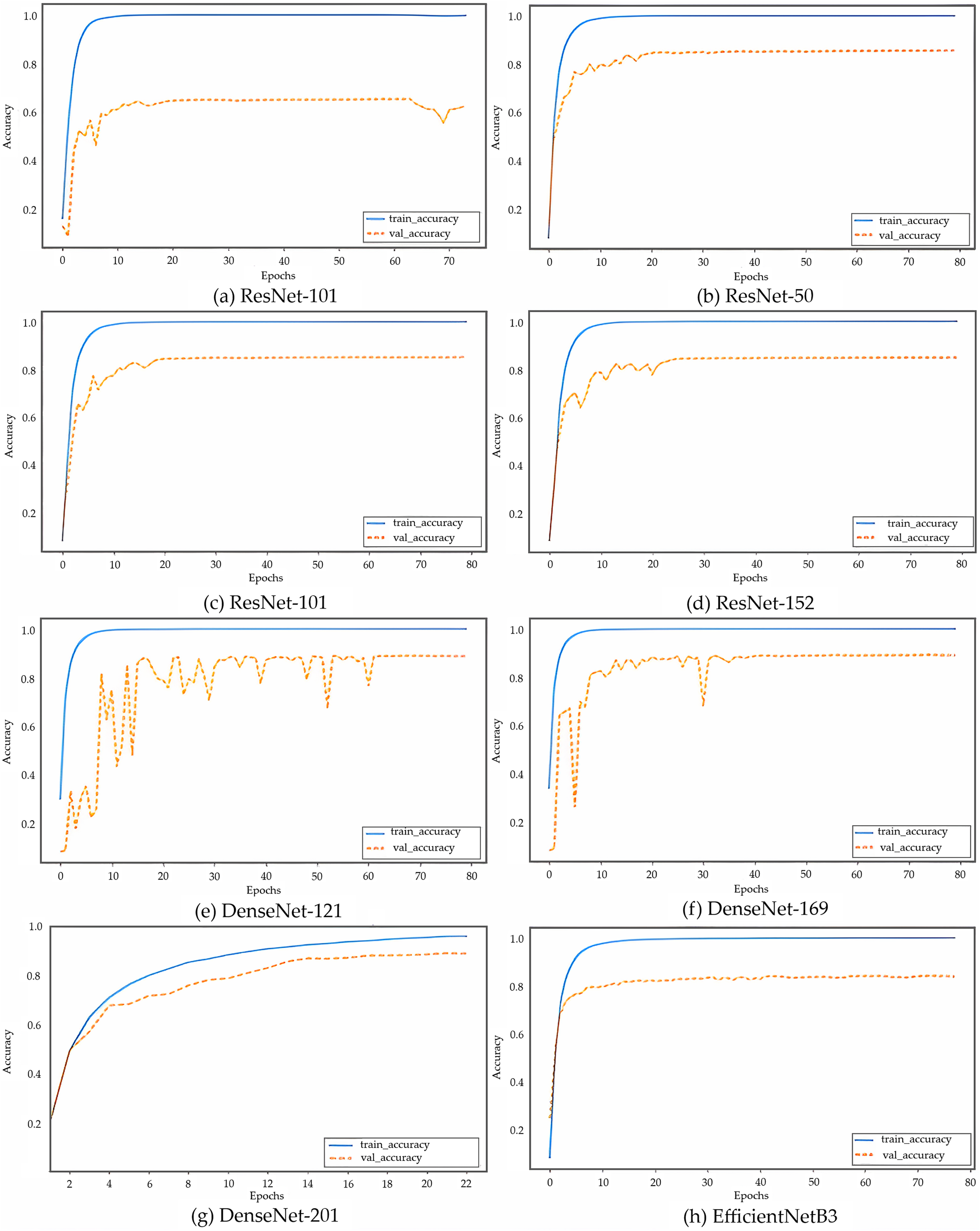
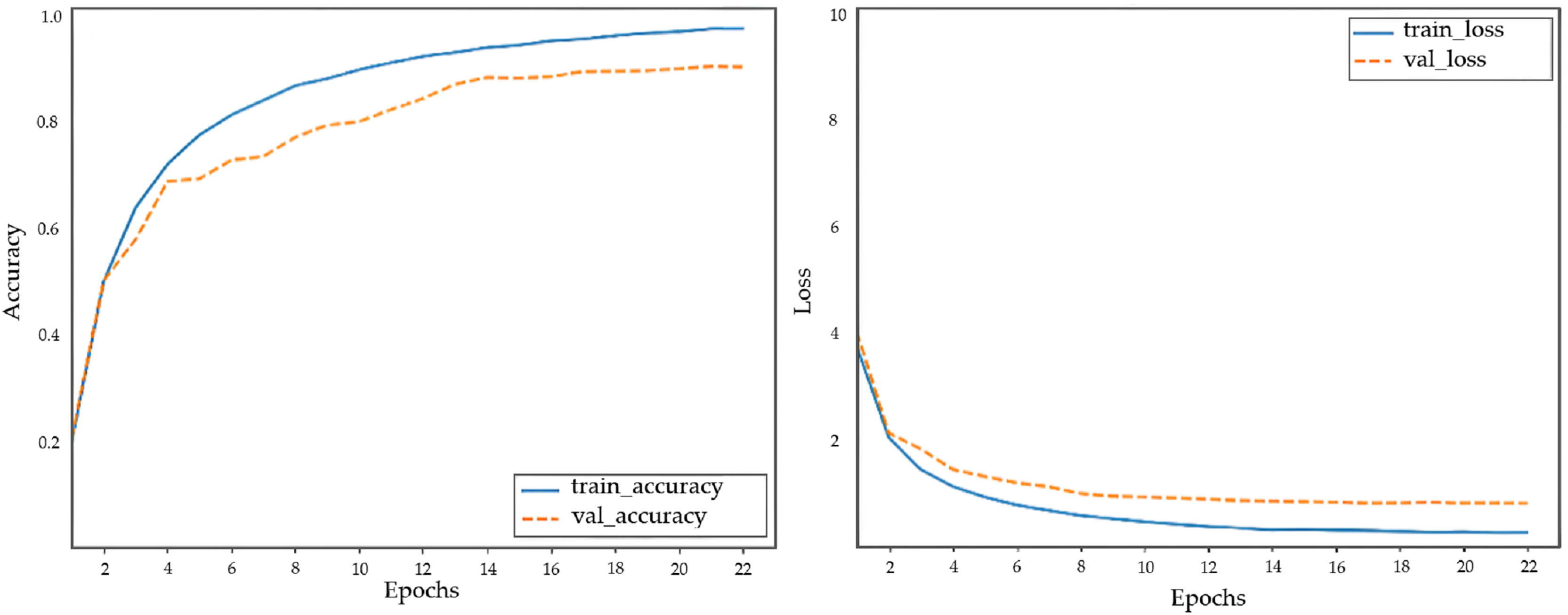
The results of the CNN models are shown in Fig. 5, where DenseNet-201 (Fig. 5G, also shown separately in Fig. 6) is clearly observed as the model with the highest performance, followed by DenseNet-169, DenseNet-121, ReseNet-50, ReseNet-101, ResNet-152, EfficientNetB3, and VGG-16, with accuracies of 0.92, 0.91, 0.91, 0.89, 0.88, 0.88, 0.87, and 0.70, respectively. The proposed model applies eight different algorithms, VGG-16, ResNet-50, ResNet-101, ResNet-152, DenseNet-121, DenseNet-169, DenseNet-201, and EfficientNetB3 to the validation set of the CC samples.
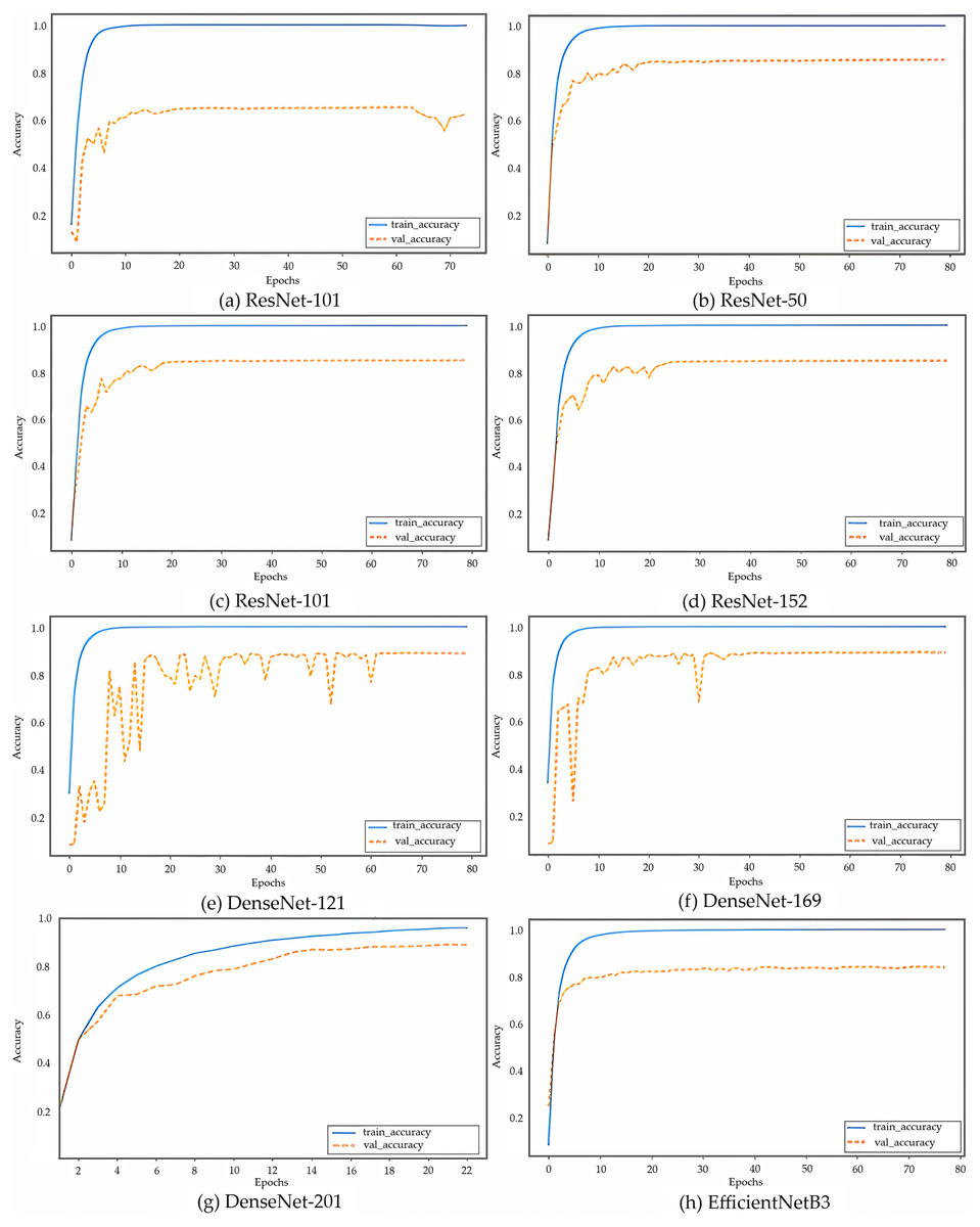
Figure 5: (A–H) Accuracy curves of the eight CNN models on CC images, with solid lines for training and dashed lines for validation.
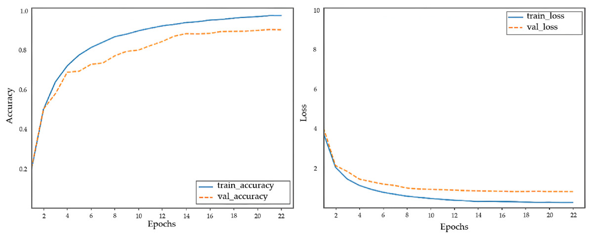
Figure 6: Accuracy and loss curves of the proposed model when using DenseNet-201.
During our experiments, the CC pixel size was an essential factor to consider. Therefore, pixel resizing while keeping the internal structures of the images intact was performed on the image data, and a suitable size was selected for further preprocessing and then passed to the CNN pipeline. Table 7 lists the impact of the resizing process on the performance of the model. From the observed results, it can be clearly observed that the size of 224 × 224 × 1 considered in our final model implementation helps to produce the highest performance compared to the other pixel resolutions.
| Scaling | Accuracy | Precision | Recall | F1-score |
|---|---|---|---|---|
| 75 × 75 × 1 | 0.86 | 0.86 | 0.86 | 0.86 |
| 150 × 150 × 1 | 0.90 | 0.90 | 0.90 | 0.90 |
| 224 × 224 × 1 | 0.92 | 0.92 | 0.93 | 0.92 |
| 75 × 75 × 3 | 0.85 | 0.85 | 0.86 | 0.85 |
| 150 × 150 × 3 | 0.90 | 0.90 | 0.90 | 0.89 |
| 224 × 224 × 3 | 0.92 | 0.92 | 0.92 | 0.91 |
The most commonly used machine learning evaluation metrics were considered to evaluate the performance of the different models. As shown in Table 8, these models exhibited various performances, with the DenseNet-201 method exhibiting the highest performance and VGG-16 exhibiting the lowest. DenseNet-201, which is used in our proposed model, had an accuracy of 0.92, precision of 0.92, recall of 0.93, and F1-score of 0.92.
| Models | Accuracy | Precision | Recall | F1-score |
|---|---|---|---|---|
| VGG-16 | 0.70 | 0.70 | 0.70 | 0.69 |
| ResNet-50 | 0.89 | 0.89 | 0.89 | 0.88 |
| ResNet-101 | 0.88 | 0.88 | 0.89 | 0.88 |
| ResNet-152 | 0.88 | 0.88 | 0.89 | 0.88 |
| DenseNet-121 | 0.91 | 0.91 | 0.92 | 0.91 |
| DenseNet-169 | 0.91 | 0.91 | 0.92 | 0.91 |
| DenseNet-201 | 0.92 | 0.92 | 0.93 | 0.92 |
| EfficientNetB3 | 0.87 | 0.87 | 0.88 | 0.87 |
Implementation of mobile application
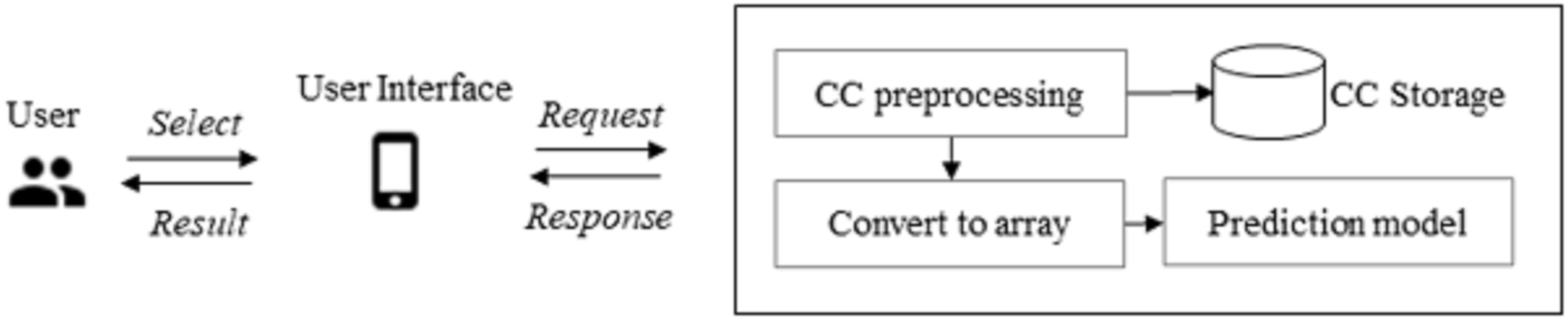
This section describes the actual implementation of the model in a mobile application and the test results obtained. The CC image prediction system consists of image preprocessing and prediction. The CC preprocessing phase comprises two steps: CC preprocessing and conversion to an array. Image preprocessing includes techniques for cleaning the CC images. The prediction phase accurately predicts the CC images. A wireless local area network was configured during the implementation to allow wireless communication between the mobile client and the server. In this study, one PC was used as a server and another as the client-side (mobile interface). The mobile device was running on a virtual device with Android version 9 and the model’s name Nexus 5X, API 28. The server was built using the Flask web framework provided in Python. The application’s SDK was 30, and the minimum version was 16, implemented in Android Studio.
Figure 7 gives an overview of the proposed implementation. Image preprocessing produces image features in the form of an array from an input CC image. First, the user inputs the CC image onto the user interface of the application. Then, the image undergoes preprocessing carried out by five modules: conversion of RGB to grayscale, Otsu’s method application, image normalization, image resizing, and conversion to an array. Converting an RGB image to grayscale transforms the image into one dimension. The one-dimensionally transformed image has the non-CC background removed, dividing the image values into two classes: CC and background. The image on which Otsu’s method is performed is converted to values between zero and one by image normalization. The normalized image is then resized to 224 × 224 pixels, saved, and converted to an array representation.
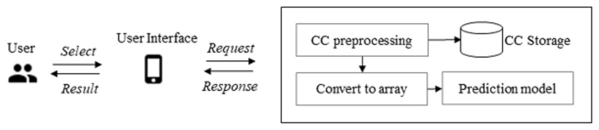
Figure 7: CC prediction implementation overview.
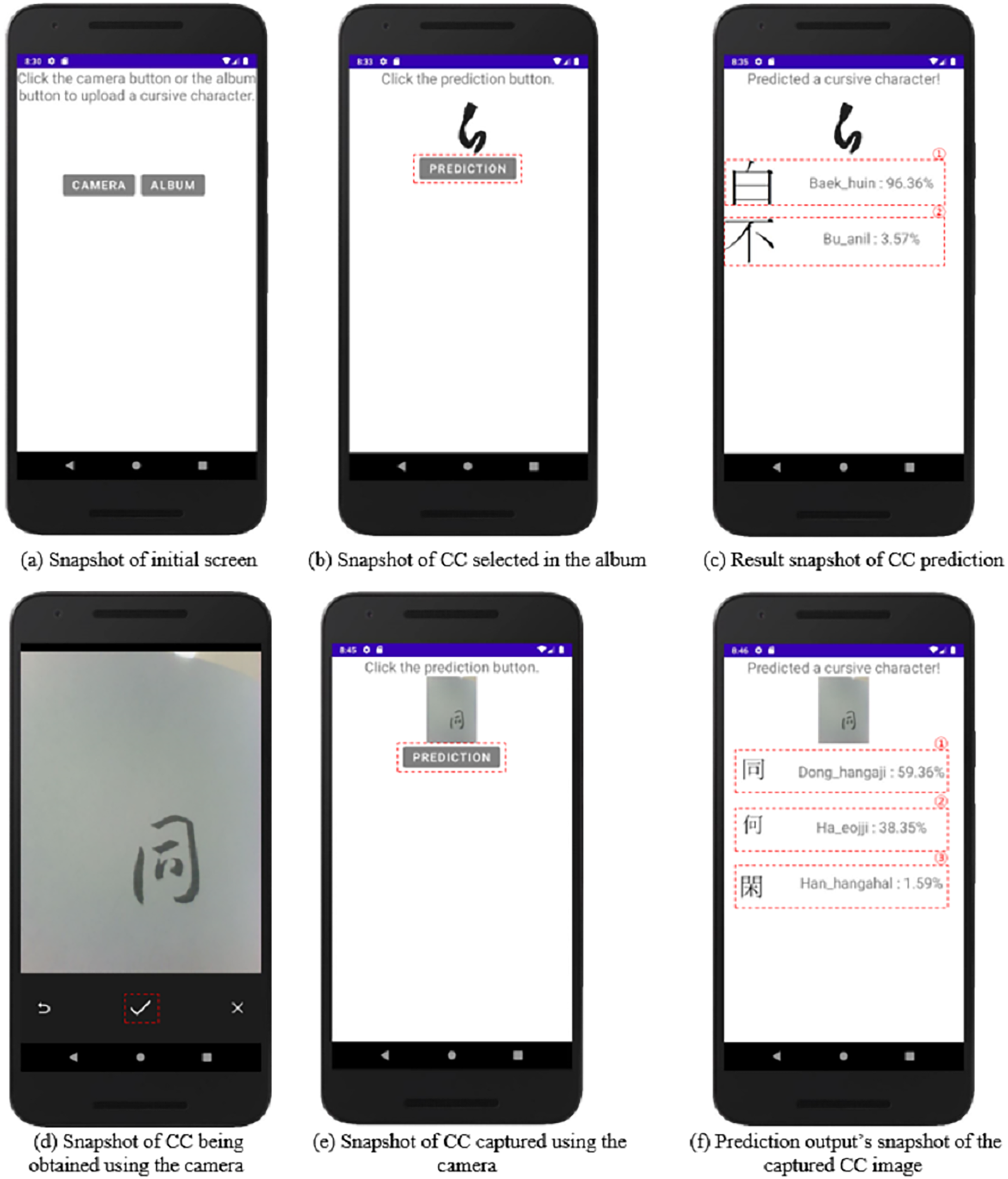
Figure 8 depicts the CC image prediction application as a snapshot of an Android smartphone. Figure 8A shows the initial screen, which has a camera button, an album button, and text instructions. Figure 8B depicts the CC chosen after clicking the album button. When the prediction button in Fig. 8B is clicked, the prediction result for the CC selected by the user is obtained, as shown in Fig. 8C. When the application loads the image and the predicted button is clicked, a request for the image is sent to the server. The predicted value of Fig. 8C-① yields a baek-huin class result of 96%, and the predicted value of Fig. 8C-② yields a bu-anil class result of 3%.
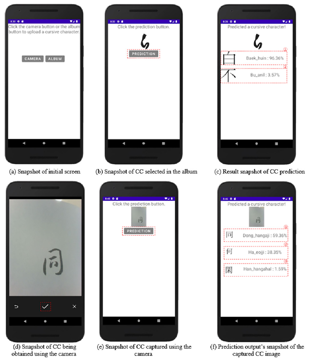
Figure 8: (A–F) Snapshots of CC prediction implementation.
Figure 8D shows what happens if the user clicks the camera button to capture a picture of a CC. Figure 8E shows the captured image on the screen; then, the prediction button is clicked to obtain the result shown in Fig. 8F. The prediction value of Fig. 8F-① yields the dong-hangaji class result of 59%, the prediction value of Fig. 8F-② yields the ha-eojji class result of 38%, and the prediction value of Fig. 8F-③ yields the han-gahalhan class result of 1%. As the resulting values are similar, the user can select the desired result. The resulting values are sorted by class in descending order from the first to the fifth, and if the value is less than one, no output is generated. The resulting image contains the output for each CC, allowing the desired CC result to be obtained. The result value responds to Android and displays the result to the user.
Discussion
The study focused on CC data and the application of different CNN models to select the algorithm with the highest prediction accuracy. Image preprocessing was performed on the CC image samples to obtain appropriate training samples. To predict CC, eight CNN models were compared, optimization was performed to improve the performance of the model, and it was implemented on a virtual Android emulator.
In this study, we used augmentation in our dataset. However, we performed augmentation except for classes with small sample size. This is because classes with insufficient data were removed to improve the accuracy. As a result, only 331 of 527 classes were used in the experiment. Therefore, our implementation could predict only 331 CC classes. In addition, our study has a limitation in predicting only one CC at a time. To address this issue, we plan to perform predictions even when inputting multiple CCs. We intend to recognize multiple CCs by predicting individual CCs separately. However, this study did not implement a model that predicts multiple CCs because the goal was to predict only one CC.
We also quantitatively and qualitatively compared our results with those of previous studies. The previous studies by Chandio, Asikuzzaman & Pickering (2020), Clanuwat et al. (2018), Shi, Bai & Belongie (2017), Qin et al. (2020), and Hong & Kim (2020) were included for comparison. Table 9 compares the quantitative and qualitative results of this study with those of other studies. We begin with a quantitative comparison of the performance of the proposed model with those of five studies. The precision, recall, and F1-score evaluation metrics were used to evaluate the performance of the models. Using 104 classes, the highest precision, recall, and F1-score across the six studies were 0.90, 0.91, and 0.91, respectively. However, using 331 classes, our proposed model received scores of 0.92, 0.93, and 0.92 for precision, recall, and F1-score, respectively. Despite a large number of classes, from the evaluation results obtained, it can be seen that our proposed model was superior to the other models.
| Research | Network | Dataset | Classes | Accuracy | Precision | Recall | F1-score |
|---|---|---|---|---|---|---|---|
| Chandio, Asikuzzaman & Pickering (2020) | Baseline + MSFA + MLFF Network | Urdu natural scene text dataset, Chars74k, ICDAR03 | 104 | – | 0.90 | 0.91 | 0.91 |
| Clanuwat et al. (2018) | U-net | Kuzushiji | 4,645 | – | 0.86 | 0.84 | 0.85 |
| Shi, Bai & Belongie (2017) | VGG-16 | SynthText, ICDAR2015, MSRA-TD500, ICDAR2013 | – | – | 0.86 | 0.70 | 0.77 |
| Qin et al. (2020) | VGG-16 | ICDAR2015 | – | – | 0.90 | 0.75 | 0.81 |
| Hong & Kim (2020) | DenseNet-201 | Caoshu | 527 | 0.88 | 0.81 | 0.84 | 0.83 |
| Our approach | DenseNet-201 | CC dataset | 331 | 0.92 | 0.92 | 0.93 | 0.92 |
The following sections provide qualitative comparisons of the datasets used in each study. The Urdu natural scene text dataset is a collection of 18,500 images containing Urdu text. Char74k is composed of synthetically generated single-character images and natural scene images of Kannada characters. ICDAR contains text images of incidental scenes shot with Google Glasses without regard to location, quality of the site, or viewpoint. SynthText dataset was created by combining natural images with rendered text in various fonts, sizes, orientations, and colors. The Kuzushiji dataset is due to the unique structure of the Japanese language, which at the time consisted of two types of character sets, a phonetic alphabet, and non-phonetic kanji characters. The dataset contains 4,645 classes. The Caoshu dataset contains CC characters in Chinese. There are 527 classes, and there is an issue of data imbalance. The Caoshu dataset closely resembles our dataset. However, in our study, classes with insufficient data were removed to address the data imbalance problem, and the data imbalance issue was addressed through data augmentation. Our proposed model achieved higher results in terms of accuracy, precision, recall, and F1-score than those reported by Hong & Kim (2020).
Despite the commendable performance of the proposed model and its successful deployment as a mobile application, three main limitations remain. First, while the proposed model leveraging transfer learning demonstrated superior predictive performance, this study did not conduct an in-depth analysis to explain why the proposed model outperformed alternative methods. Future work will explore model interpretability to better understand why the proposed architecture works better. Second, while the mobile application enables real-time CC prediction, formal usability studies and latency benchmarks were not performed. Future research will assess the application’s responsiveness, user experience, and robustness across various conditions. Third, to address data imbalance, image augmentation was employed to enhance training stability and generalizability. While this approach proved effective, future work will consider integrating synthetic oversampling techniques, such as SMOTE or GAN-based methods, to further enhance the representation of minority classes and perform a comparative analysis to show the most effective approach among them.
Conclusions
This article presented a proposed CC prediction approach using a smartphone with integrated deep learning technology. The image preprocessing step allows the system to make more accurate predictions. The performance of the proposed algorithm was compared with that of VGG-16, ResNet-50, ResNet-101, ResNet-152, DenseNet-121, DenseNet-169, DenseNet-201, and EfficientNetB3 for the same purpose. Based on the experimental results of the proposed methods on the CC datasets, our model using DenseNet-201 achieved the highest performance with accuracy, precision, recall, and F1-score of 92%, 92%, 93%, and 92%, respectively. To avoid biases among image samples, they were uniformly resized and converted to grayscale to reduce computational requirements. Noise was removed using Otsu’s method. The CC images used in the experiments had a shape of 224 × 224 × 1, the number of classes in the dataset was 331, and data imbalance was resolved using image augmentation. SGD optimization methods have shown considerable improvement with the finetuning of our hyperparameters in our model performance.
The current implementation uses one CC as the input data to show multiple predicted results to the user. Users can input the CC from a photo album or via the camera. The prediction using an album or the camera yielded results of 96.36% and 59.36%, respectively. However, because the dataset consists of single CCs, the input data are limited to one CC. This issue must be addressed in the future and strengthening the dataset could be a solution. Our dataset is limited in that the CC class is limited to 331 classes. The experiments were conducted using an input image containing a single CC and producing a single prediction of the original representation of the CC. In future work, we will increase the number of recognizable characters by extracting CC data from ancient documents and books. Subsequently, we plan to extend our current model to predict the original representations from inputs with multiple CCs on the image input sample.