
Mine subsidence monitoring and prediction integrating SBAS-InSAR technology and BO-Prophet model
- Published
- Accepted
- Received
- Academic Editor
- Feng Gu
- Subject Areas
- Artificial Intelligence, Computer Vision, Data Mining and Machine Learning, Spatial and Geographic Information Systems
- Keywords
- Subsidence monitoring, SBAS-InSAR, Subsidence prediction, BO-Prophet, Coal mining
- Copyright
- © 2025 Yu
- Licence
- This is an open access article distributed under the terms of the Creative Commons Attribution License, which permits unrestricted use, distribution, reproduction and adaptation in any medium and for any purpose provided that it is properly attributed. For attribution, the original author(s), title, publication source (PeerJ Computer Science) and either DOI or URL of the article must be cited.
- Cite this article
- 2025. Mine subsidence monitoring and prediction integrating SBAS-InSAR technology and BO-Prophet model. PeerJ Computer Science 11:e3327 https://doi.org/10.7717/peerj-cs.3327
Abstract
Coal mining causes significant environmental disruptions due to excessive resource extraction. Real-time monitoring and prediction of mining-induced surface deformation are critical for ensuring mining safety. Conventional monitoring methods struggle to achieve large-scale real-time observation and have limitations in terrain adaptability and weather resistance. Conventional prediction methods are constrained as follows: numerical simulation is limited by the complexity of physical parameters; mathematical statistics requires substantial data and struggles to comprehensively reflect geotechnical properties; hybrid algorithms involve complex modeling and rely on individual models. This study develops an integrated framework combining Small Baseline Subset Interferometric Synthetic Aperture Radar (SBAS-InSAR) and Bayesian optimization-Prophet (BO-Prophet) models for mining subsidence monitoring and forecasting. Using the Yinying Coal Mine as the study area, multi-source radar datasets are processed through SBAS-InSAR. This technique identifies four major subsidence areas and generates time-series deformation data. Cross-validation confirms the reliability of SBAS-InSAR monitoring results: the Pearson correlation coefficient between ascending-orbit (Sentinel-1A) and descending-orbit (Radarsat-2) results of 3,000 high-coherence points in the subsidence area reaches 0.946; compared with four Global Navigation Satellite System (GNSS) stations, the maximum absolute errors are 4.684, 3.328, 3.194, and 2.462 mm respectively, with consistent deformation trends, and both methods confirm its reliability. Comparative analysis reveals superior prediction accuracy of the BO-Prophet model over Bayesian optimization-long short-term memory (BO-LSTM) at six characteristic points. The BO-Prophet model achieves a mean absolute error (MAE) of 2.02 mm, representing a 25.2% reduction from BO-LSTM (2.70 mm). Its root mean square error (RMSE) measures 2.36 mm, demonstrating a 35.6% reduction compared to BO-LSTM (3.67 mm). Subsidence predictions for area B using BO-Prophet show high spatial-temporal consistency with SBAS-InSAR monitoring results. Correlation analysis demonstrates a correlation coefficient (R²) exceeding 0.96 between predicted and observed values. The integration of SBAS-InSAR and BO-Prophet shows strong potential for mining subsidence monitoring and forecasting. This combined approach enhances early warning capabilities and supports disaster mitigation strategies in mining areas.
Introduction
Coal, as a crucial mineral resource in China, holds absolute dominance in the national energy structure and plays an irreplaceable role in social development and economic construction. Shanxi Province contributes approximately one-quarter of China’s coal production, serving as a vital national energy base (Bai et al., 2020). However, excessive coal mining has triggered ground collapse, air pollution, farmland destruction, and geological hazards like landslides and mudslides, severely threatening local residents’ safety and quality of life (Chu & Muradian, 2016; Dontala, Reddy & Vadde, 2015; Habib & Khan, 2021). Real-time monitoring and prediction of surface deformation are essential for preventing geological disasters and ensuring mining safety.
Traditional monitoring methods like precise leveling and GPS measurements face limitations in terrain adaptability, weather resistance, and spatial coverage (Santos, Cabral & Pontes Filho, 2012; Sevil, Benito-Calvo & Gutiérrez, 2021). These point/line-based approaches struggle to achieve large-scale monitoring and fail to reflect comprehensive deformation patterns across mining areas. High costs, low efficiency, and limited coverage further restrict their application in long-term, large-area subsidence monitoring.
Interferometric synthetic aperture radar (InSAR) overcomes these limitations by enabling cost-effective, weather-independent large-area monitoring with comprehensive surface deformation insights (Aobpaet et al., 2013; Wu, Wei & D’Hondt, 2022). D-InSAR generates interferograms to separate terrain features from deformation signals, supporting continuous long-term monitoring (Fan et al., 2011; Zhu et al., 2024). However, its accuracy suffers from image decorrelation and atmospheric delays (Cai et al., 2023). PS-InSAR achieves high-precision deformation monitoring by identifying persistent scatterers (buildings, bare rocks) with stable phase characteristics, which effectively mitigates atmospheric phase errors. However, in mining areas with high vegetation coverage, the scarcity of such persistent scatterers leads to sparse monitoring points, failing to capture the overall subsidence patterns (Liu et al., 2022). DS-InSAR improves monitoring point density by identifying distributed scatterers (vegetated areas with weak scattering targets), particularly outperforming PS-InSAR in vegetated zones. However, it still struggles with spatial decorrelation in steep terrains or areas with severe atmospheric delays, compromising accuracy in mountainous mining regions (Li et al., 2021). In mining area subsidence monitoring, SBAS-InSAR demonstrates strong adaptability to complex environments. For mountainous mining areas with rugged terrain and high vegetation coverage, SBAS-InSAR effectively reduces temporal and spatial decorrelation by controlling small spatiotemporal baselines. It generates continuous high-temporal-resolution deformation time series to capture dynamic subsidence from mining activities, and adapts flexibly to moderate data volumes, balancing monitoring accuracy and regional coverage (Du et al., 2021; Khan et al., 2025; Li, Xu & Li, 2022). Unlike DS-InSAR, which may fail in large deformation zones due to insufficient coherence, SBAS-InSAR maintains reliable results across diverse mining scenarios. This makes it more suitable for subsidence monitoring in such complex mining environments compared to D-InSAR, PS-InSAR, and DS-InSAR. This SBAS-InSAR approach has gained widespread recognition in mine monitoring.
Surface subsidence prediction methods include numerical simulation, mathematical statistics, Hybrid algorithms, and machine learning models (Cai et al., 2023; Wang et al., 2025). Numerical simulation methods analyze stress distribution in mining areas through numerical modeling, yet their effectiveness is limited by the complexity of physical parameters (He, Wu & Ma, 2023; Li, Zha & Guo, 2019). Mathematical statistical methods offer intuitive data-driven solutions; however, they demand substantial observational data and struggle to comprehensively characterize geotechnical medium properties, thereby compromising prediction reliability (Hejmanowski & Malinowska, 2009). Hybrid algorithms enhance accuracy and stability by integrating multiple model outputs, though they entail complex modeling structures and remain dependent on individual model performance (Shen, Santosh & Arabameri, 2023).
In recent years, machine learning models have demonstrated remarkable potential in surface deformation prediction (Deng et al., 2025; Wang et al., 2024; Yang et al., 2025), particularly in addressing multi-factor induced surface deformations. The large-scale, high-precision surface deformation data acquired through InSAR technology provides abundant training samples for machine learning models (Guo et al., 2023; Shi et al., 2020, 2023). Assessing the applicability of machine learning models for mining subsidence prediction requires comprehensive consideration of environmental characteristics and data attributes. Grey models (GM) are based on grey system theory. GM suits scenarios with limited samples or missing information. For example, Shi et al. (2020) integrated D-InSAR technology with the GM(1,1) model to achieve unified subsidence monitoring and prediction. However, GM exhibits poor prediction stability and struggles to capture nonlinear dynamic deformations. Support vector regression (SVR) can map high-dimensional nonlinear relationships and possesses good robustness. Zhang et al. (2021) successfully predicted subsidence in Shaanxi mining areas using SBAS-InSAR and SVR. Nevertheless, SVR demands substantial computational resources. It also shows insufficient adaptability to sudden subsidence events in long time series. Long short-term memory (LSTM) networks perform well in learning mining subsidence patterns. Ma, Sui & Lian (2023) confirmed through comparative experiments that LSTM outperforms SVR. However, Dongwei et al. (2024) noted LSTM’s susceptibility to spatial heterogeneity and feature deficiencies, these limitations can cause significant accuracy reductions. In contrast, the Prophet model employs Bayesian curve fitting via a generalized additive model. Prophet offers notable flexibility and robustness. Its built-in trend decomposition module accurately distinguishes subsidence caused by natural and anthropogenic factors (Bi et al., 2024).
Hyperparameter selection significantly impacts prediction model performance. Research by Chen et al. (2025) demonstrated that hyperparameter optimization effectively enhances model prediction capability. Subjective hyperparameter selection proves inefficient and often suboptimal. Therefore, this study introduces Bayesian optimization (BO) for hyperparameter tuning. This method efficiently explores the parameter space. BO achieves relatively optimal parameter combinations with fewer evaluations and lower time costs. To highlight the advantages of the proposed Bayesian optimization-Prophet (BO-Prophet) model for mining subsidence prediction, we conducted a comparative analysis. We compared its performance against Bayesian optimization-long short-term memory (BO-LSTM), an LSTM model also optimized with Bayesian optimization.
This study focuses on Yangquan’s Yinying mining area, utilizing 34 ascending Sentinel-1A radar images and 17 descending radar RADARSAT-2 images for SBAS-InSAR processing. The analysis of multi-source data from June 2023 to August 2024 confirms result consistency and reliability. To optimize prediction accuracy, Bayesian optimization adjusts hyperparameters in Prophet and LSTM models. The enhanced models predict subsidence values at selected characteristic points, comparing performance outcomes to provide scientific support for early warning systems.
Study area
Yinying Coal Mine is located in Yinying Town, northern suburbs of Yangquan City. Its geographic coordinates range from 113°27′17.46″E to 113°33′27.684″E longitude and 37°56′22.754″N to 38°0′36.407″N latitude. The area features a temperate continental monsoon climate with annual average temperatures between 8–12 °C and precipitation ranging 450–550 mm.
The terrain shows northwest-high and southeast-low topography, classified as low mountain hills with elevations spanning 660–1,373 m. Surface coverage primarily consists of forest land and grassland. The mining area covers approximately 19.1 km2.
As a major coal production base, Yinying Coal Mine maintains an average coal seam thickness of 3.75 m. Coal seams exhibit an average dip angle of approximately three degrees. Annual production capacity reaches 2.4 million tons.
Key geological characteristics include crisscrossing valleys and densely distributed gullies formed by historical river erosion. These geomorphological features contribute to complex mining conditions requiring advanced monitoring systems like SBAS-InSAR for deformation tracking. Figure 1 shows the geographical location and surface conditions of the study area.
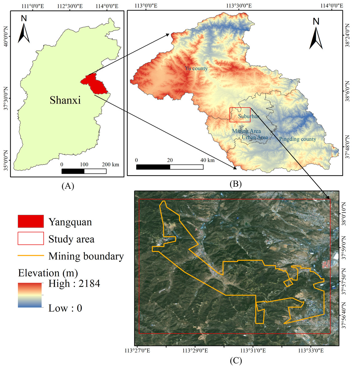
Figure 1: Location and current status of the study area: (A) Shanxi province; (B) DEM of Yangquan City; (C) study area (red box), Yinying Mining Boundary (orange line).
Satellite image base map from TianDiTu (www.tianditu.gov.cn).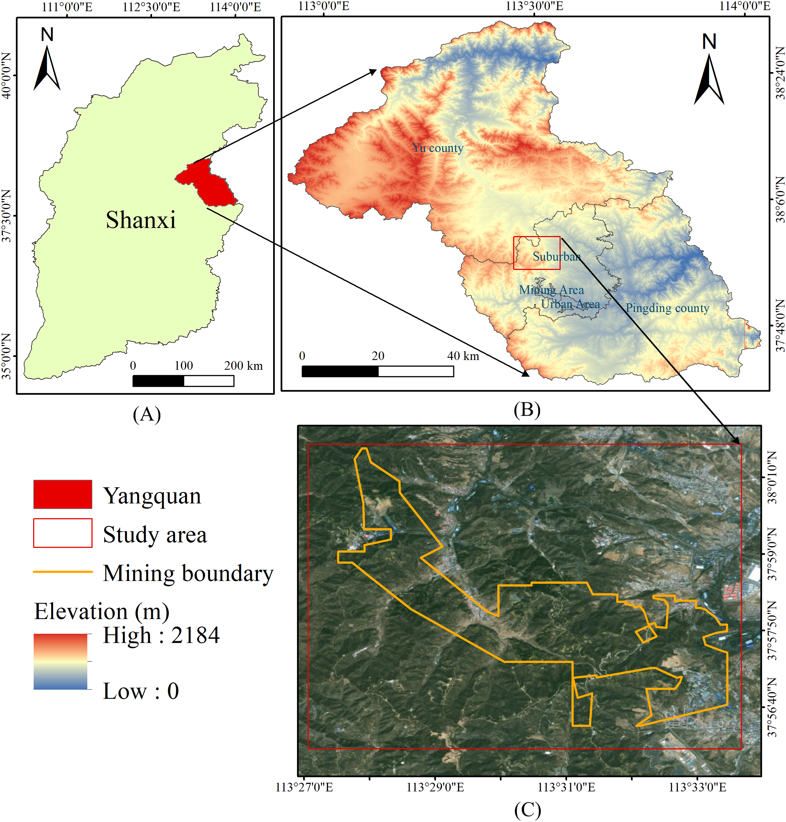
Data sources and methodology
Data sources
This study collected ascending synthetic aperature radar (SAR) data from June 23, 2023 to August 4, 2024 and descending SAR data spanning June 21, 2023 to August 2, 2024. The descending data is used to verify the reliability of ascending monitoring results. The ascending dataset comprises 34 scenes of Sentinel-1A IW-mode images with 20 m spatial resolution. Its 12-day revisit cycle ensures temporal consistency for deformation monitoring. Descending data contains 17 scenes of RADARSAT-2 XF-mode images achieving 5 m resolution. The 24-day revisit cycle provides complementary observation angles. In addition, Precise orbit files were collected to eliminate orbital errors through ESA’s Precise Orbit Determination (POD) service. A total of 30 m digital elevation model (DEM) data were obtained to remove topographic phase effects. Table 1 shows the comparison between the two types of data.
| Sensor | Orbital direction | Revisit time | Polarization mode | Imaging mode | Resolution |
|---|---|---|---|---|---|
| Sentinel-1A | Ascending | 12d | VV + VH | IW | 5 m * 20 m |
| RADARSAT-2 | Descending | 24d | HH | XF | 5 m * 5 m |
SBAS-InSAR
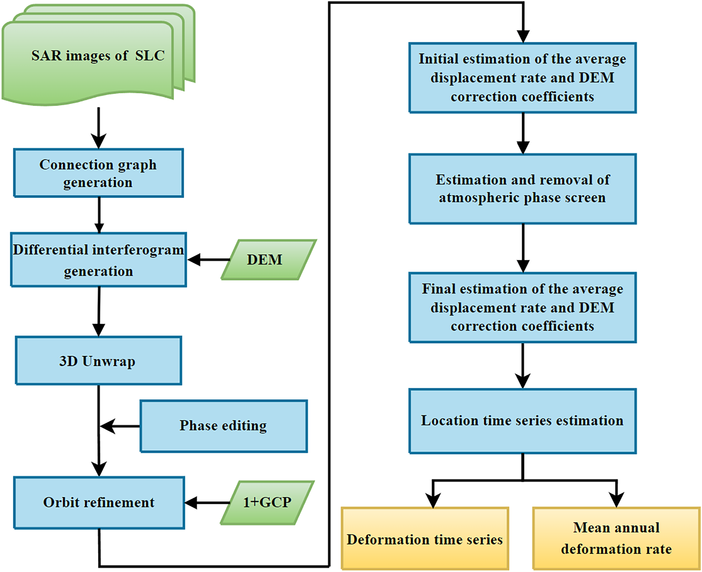
SBAS-InSAR (Small Baseline Subset InSAR) is a time-series InSAR analysis method using multiple master images, Berardino et al. (2002) proposed this technology in 2002. Figure 2 shows the SBAS-InSAR workflow. The core principle involves organizing numerous SAR datasets into interferometric subsets. Each subset contains multiple master images. All interferometric pairs in a subset maintain baseline lengths below critical baseline thresholds. The time baselines are also minimized. This approach resolves decorrelation issues in both temporal and spatial dimensions. The method then applies minimum norm criteria for deformation velocity estimation. Singular value decomposition (SVD) helps obtain time-series deformation of coherent targets. It also generates average deformation rate maps (Li, Xu & Li, 2022). SBAS-InSAR achieves reliable monitoring results with relatively small datasets. This technology proves particularly effective for monitoring surface deformation in mining areas.
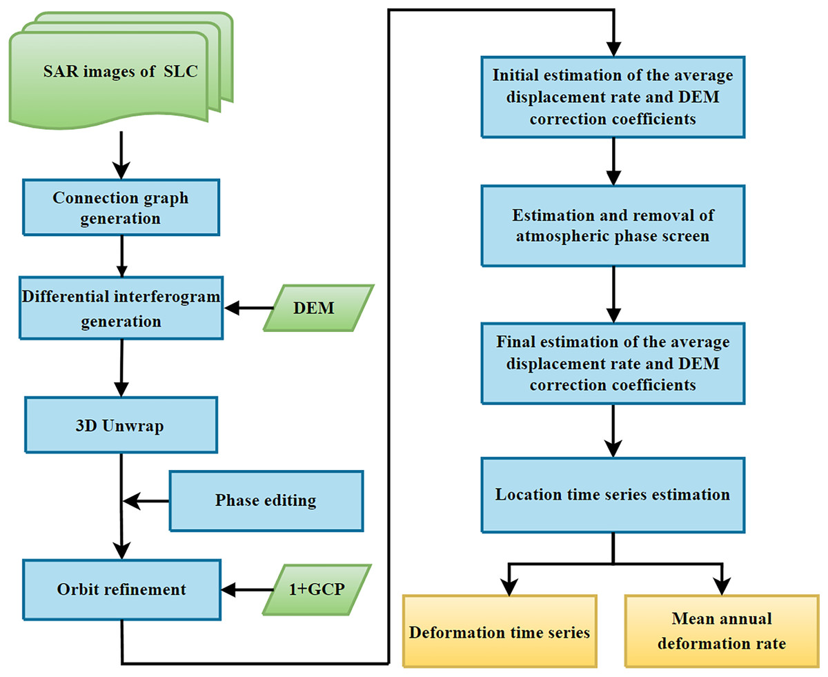
Figure 2: SBAS-InSAR processing flow chart.
BO-Prophet prediction model
This study builds BO-Prophet and BO-LSTM models using PyCharm and Python 3.8, primarily employing the Pandas, NumPy, Kats and Ax libraries. The BO-Prophet model combines Bayesian optimization and the Prophet forecasting framework. Facebook released Prophet as an open-source time series prediction tool in 2017 (Taylor & Letham, 2018).
The Prophet model uses an additive regression framework. It consists of three core components: trend, seasonality, and holiday effects. This structure enables Prophet to handle diverse forecasting problems with unique characteristics (Chang, Yang & Zhang, 2025; Chérif et al., 2023). It effectively captures trend changes, seasonal patterns, holidays, and irregular events in time series data. The basic formula of the Prophet model is:
(1)
In the formula, represents the trend component, modeling non-periodic changes using piecewise linear or logistic regression; denotes the seasonality component, capturing periodic fluctuations like weekly or yearly cycles; accounts for holiday effects, addressing impacts from special events; is the error term, and it is used to represent unpredicted random fluctuations.
The logistic growth model employs a sigmoid function to describe growth patterns. The logistic function (sigmoid) is expressed as:
(2)
In the formula, indicates the trend’s saturation capacity; controls the growth rate; represents the base inflection point parameter of the trend; serves as the trend’s changepoint indicator matrix; represents the trend slope adjustment coefficient; represents the trend inflection point time adjustment coefficient.
Prophet incorporates Fourier series to model periodic variations. This approach represents seasonality through linear combinations of sine and cosine functions:
(3)
In the formula, , represent the Fourier coefficients; indicates the period length; serves as the Fourier basis matrix; denotes parameters following a normal distribution: β ~ N (0, σ2); A larger σ amplifies seasonal effects, while a smaller σ reduces them.
Hyperparameters are parameters set before training machine learning models. Their values cannot be learned automatically during training. Researchers select these values based on experience or experimentation (Bischl et al., 2023). Manual hyperparameter adjustment is time-consuming and expertise-dependent. BO is an algorithm for finding optimal solutions to functions. It efficiently explores parameter spaces. This method identifies strong parameter combinations with minimal trials and time. It is widely used for hyperparameter tuning in machine learning (Snoek, Larochelle & Adams, 2012). BO builds a probabilistic model of the objective function. This model guides the search process. The goal is to find parameter configurations that optimize the objective function. The algorithm handles complex objective functions with multiple peaks or non-convex shapes. It performs effectively in many practical applications (Shahriari et al., 2015).
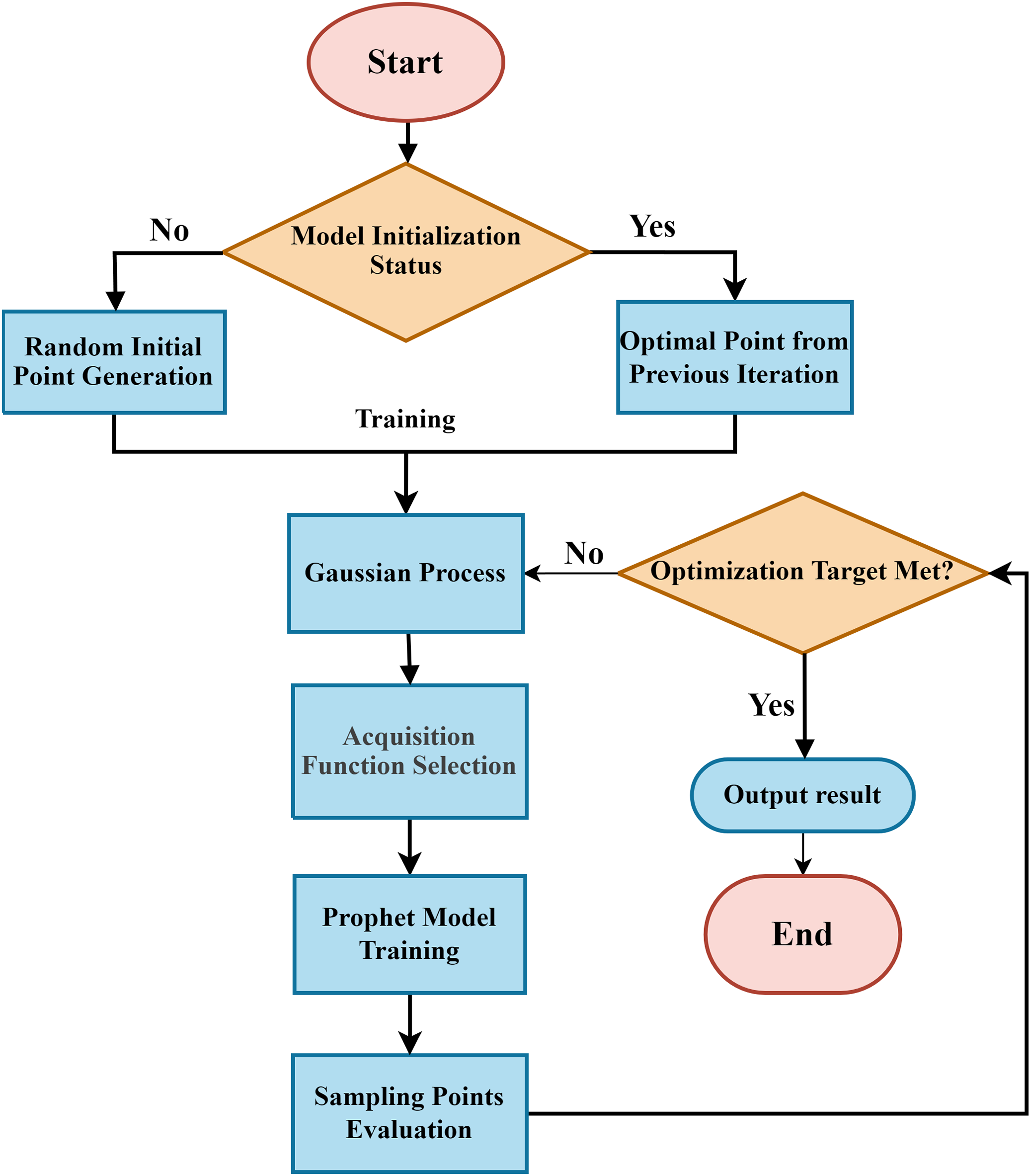
The BO-Prophet framework applies BO to tune Prophet hyperparameters, as shown in Fig. 3. The process begins by randomly sampling an initial set of hyperparameters. These hyperparameters initialize the model configuration. The framework then evaluates the model training outcomes using predefined metrics. A Gaussian process model integrates historical hyperparameter evaluations and their performance results. An acquisition function analyzes this probabilistic model. It selects the next hyperparameter set with the highest potential performance improvement. The system iteratively repeats hyperparameter selection, model retraining, and performance evaluation. This loop continues until meeting predefined termination criteria (e.g., maximum iterations or convergence thresholds).
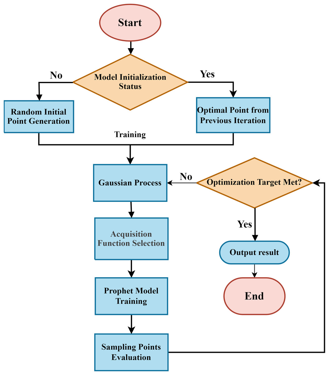
Figure 3: Flowchart of Prophet prediction model algorithm based on Bayesian optimization.
LSTM prediction model
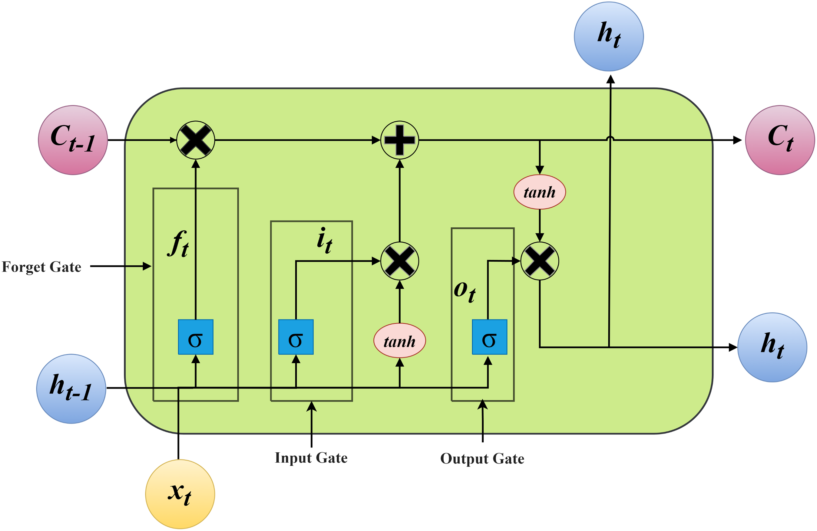
This study compares the LSTM neural network prediction model with the Prophet model. LSTM represents a specialized type of recurrent neural network (RNN) (Yu et al., 2019). Compared to conventional RNNs, LSTM demonstrates superior performance in processing time-series data with extended intervals between critical events. The LSTM architecture incorporates memory cells and three gating units. Memory cells store historical information systematically. The input gate regulates the integration of current input data into memory cells. The forget gate manages the elimination of irrelevant information from memory cells (Smagulova & James, 2019). The output gate controls the transmission of stored information to subsequent layers. These gating mechanisms collectively preserve crucial temporal patterns in sequences. They effectively address long-term dependency challenges in time-series analysis. Additionally, this structure resolves gradient-related instability problems common in standard RNNs. Figure 4 illustrates the memory unit configuration of the LSTM neural network.
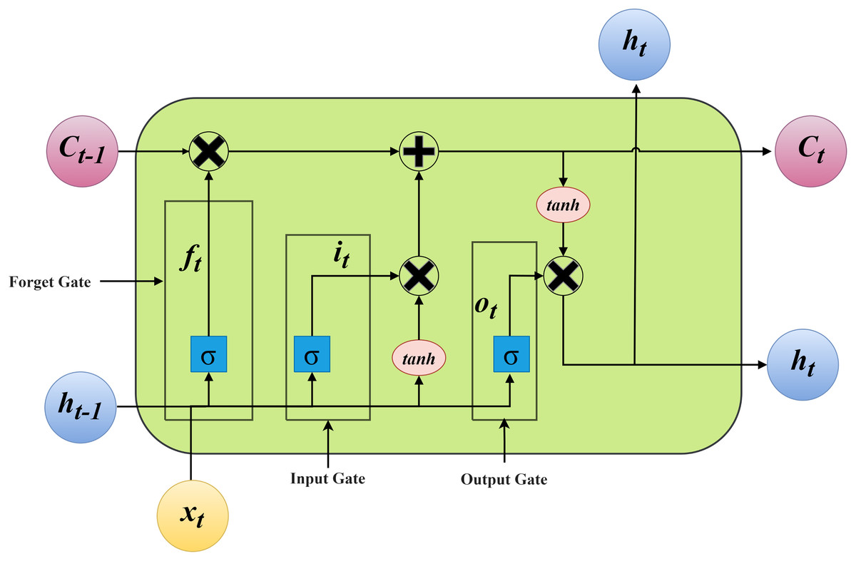
Figure 4: LSTM unit structure.
The memory unit structure of LSTM neural networks can be mathematically represented by the following equations:
(4)
(5)
(6)
(7)
(8)
(9)
In the formulas, the notation represents the concatenated matrix of the previous hidden state and current input . The variables , , and denote the forget gate, input gate, and output gate values at time step t. The operator indicates the Sigmoid activation function. , and are the weight matrices of the forget gate, input gate and output gate, respectively; is the weight matrix for the candidate memory cell , acting on the concatenated matrix . , and are the bias terms of the forget gate, input gate and output gate, respectively; is the bias term for the candidate memory cell . represents the memory cell state at time step t, which retains long-term information by integrating the previous cell state and the candidate cell state .
SBAS-InSAR monitoring results and analysis
Mine surface subsidence monitoring and identification
This study processed 34 Sentinel-1A images covering the study area (June 23, 2023–August 4, 2024) using SBAS-InSAR technology. To effectively reduce temporal and spatial decorrelation, the temporal baseline threshold was set to 120 days. The spatial baseline threshold was controlled within 3% of the critical baseline. This configuration generated 134 interferometric pairs (Fig. 5).
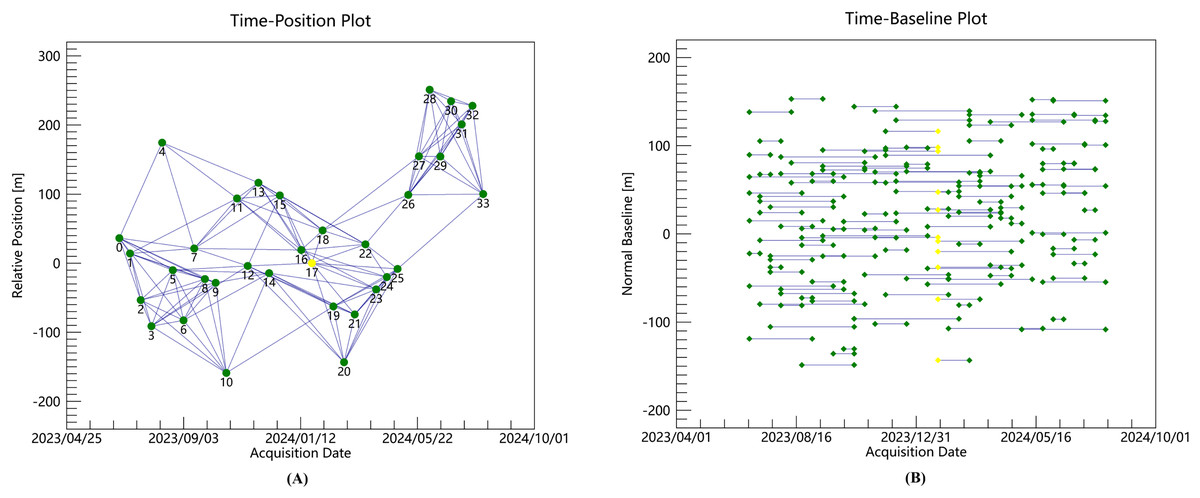
Figure 5: (A) The spatial baseline of each interferometric pair; (B) the temporal baseline of each interferometric pair.
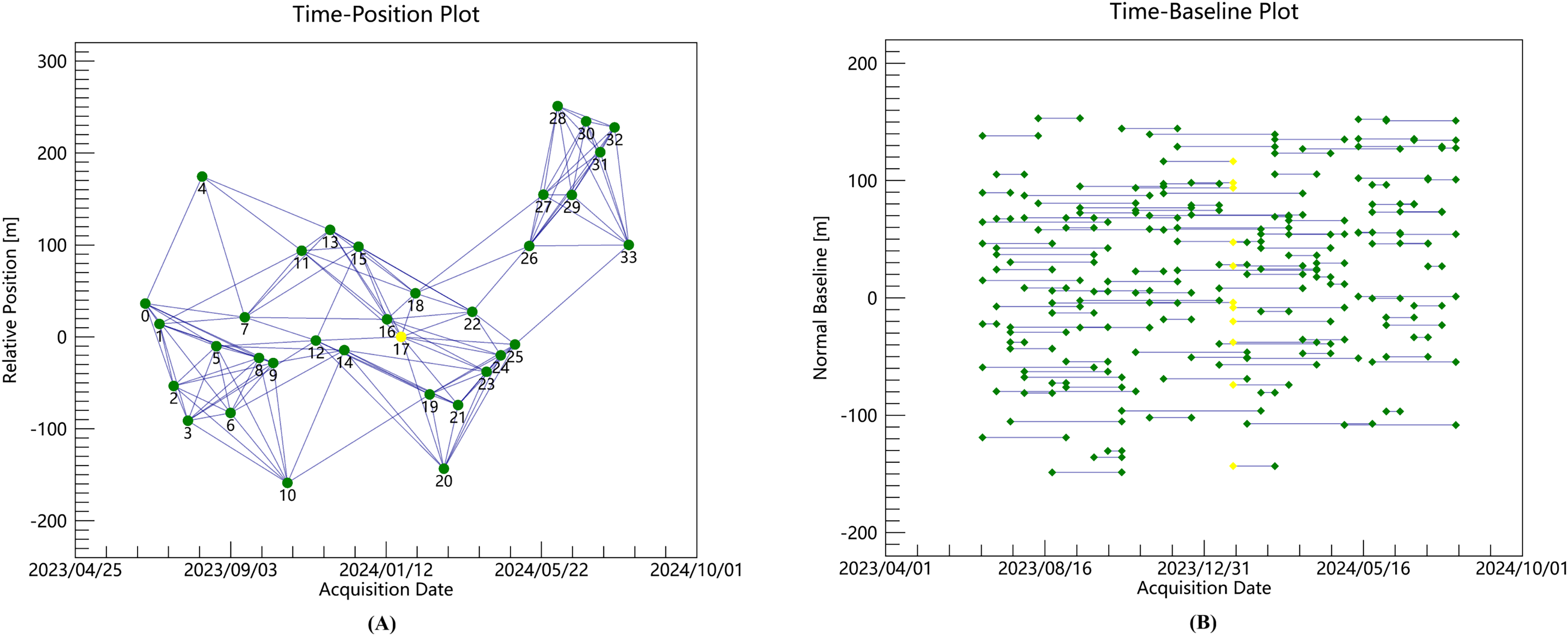
During data processing, a coherence threshold of 0.3 was applied. This threshold selected high-coherence points to ensure stability for subsequent analysis. A 30-m resolution DEM of the study area was introduced. This DEM removed topographic phase contributions. Goldstein filtering optimized the interferogram quality. Phase unwrapping was completed using the minimum cost flow (MCF) method.
Atmospheric delay and residual topographic errors were addressed through two SBAS-InSAR inversion iterations. The first inversion separated atmospheric phase from deformation signals. The second inversion further corrected residual errors. This iterative approach effectively enhanced deformation extraction accuracy.
Vertical deformation dominates surface movements in mining areas. This dominance justifies converting line-of-sight (LOS) displacements to vertical deformations. The processing yields annual average vertical deformation rate and cumulative settlement time series for Yinying Coal Mine.
Figure 6 displays the annual deformation rate map of the study area from June 23, 2023 to August 4, 2024. The figure reveals annual deformation rate ranging from −115 to 28 mm/yr. The maximum subsidence rate reaches −115 mm/yr. Four distinct subsidence areas are identified in the study area. Subsidence areas A and B are located within the mining boundaries of Yinying Coal Mine. Subsidence areas C and D occur in adjacent mining areas. Area A covers 1.04 km2, and Area B spans 0.64 km2. Field investigations confirm both areas are active coal mining zones. The observed subsidence patterns align with on-site geological conditions.
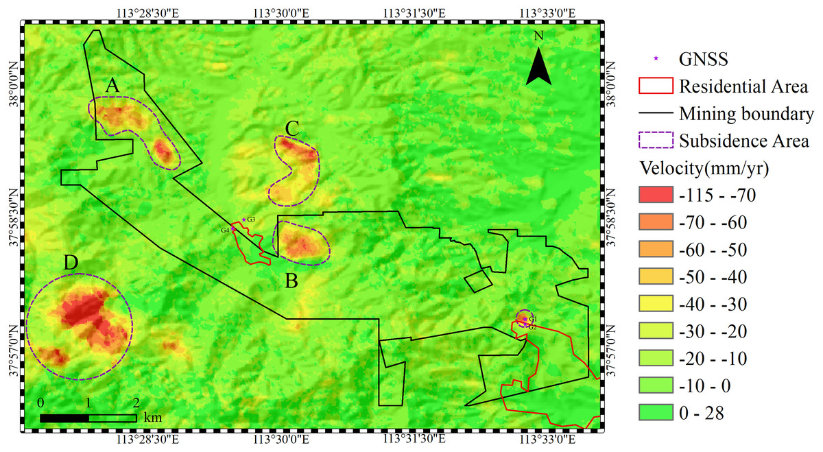
Figure 6: Deformation rate map of the study area (negative values indicate subsidence; positive values indicate uplift).
Terrain shading base map from TianDiTu (www.tianditu.gov.cn).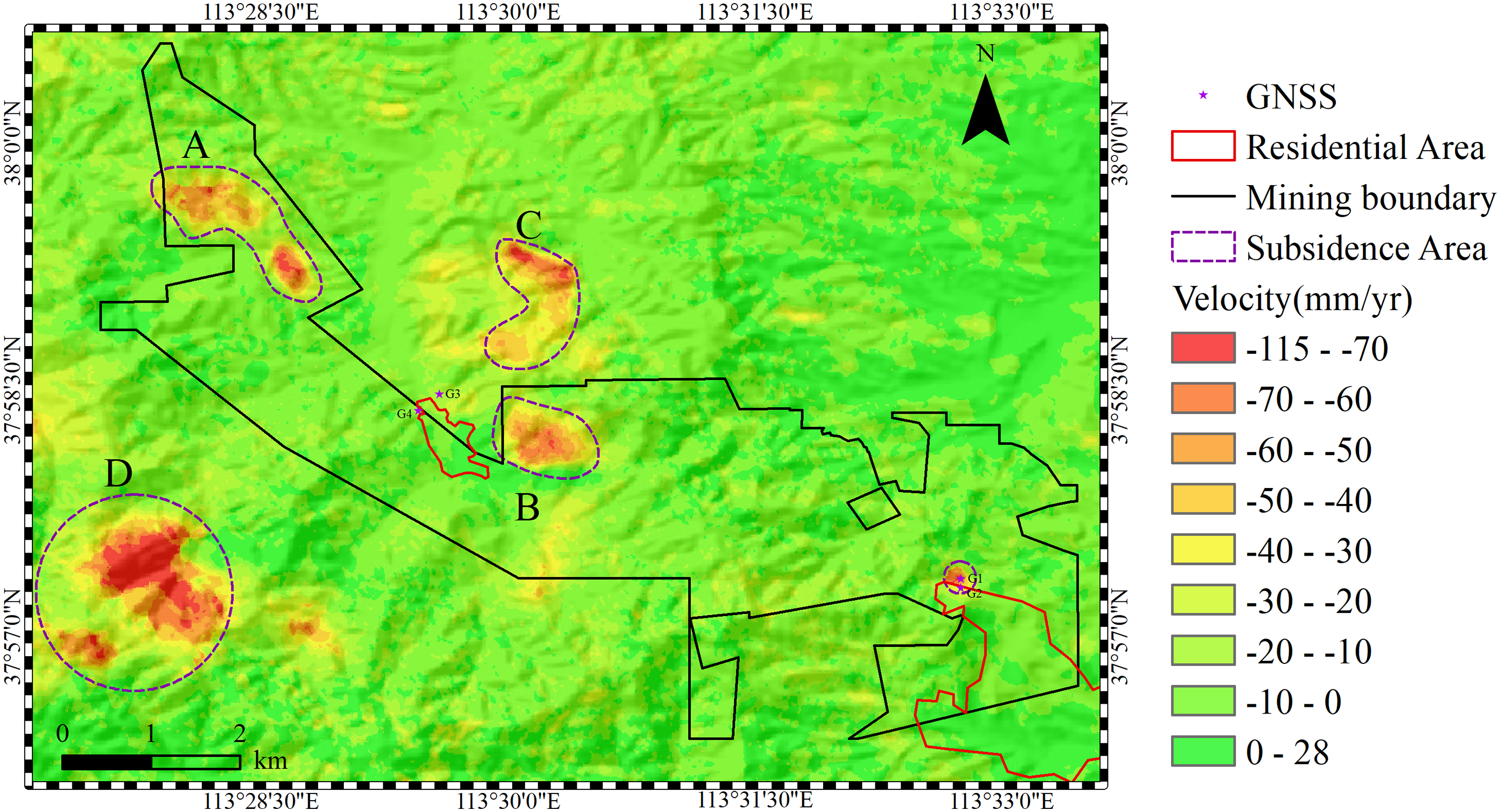
Reliability analysis of monitoring results
To validate the reliability of ascending-orbit SBAS-InSAR monitoring results, this study employed dual validation methods: cross-validation using ascending/descending data and comparison with Global Navigation Satellite System (GNSS) measurements (Tran et al., 2020; Chen et al., 2025). First, 17 descending-orbit RADARSAT-2 images (June 21, 2023 to August 2, 2024) were processed using SBAS-InSAR with consistent parameters (120-day temporal baseline, 3% spatial baseline threshold, 0.3 coherence threshold), generating 36 interferometric pairs with the December 30, 2023 image as the master image. Processing steps followed the same workflow as “Mine Surface Subsidence Monitoring and Identification”, including DEM-based flat-earth phase removal, Goldstein filtering, MCF unwrapping, and two inversion iterations for error correction.
Comparative analysis extracts 3,000 high-coherence points from subsidence areas. Figure 7 demonstrates agreement between ascending (Sentinel-1A) and descending (RADARSAT-2) orbit SBAS-InSAR results. The Pearson correlation coefficient reaches 0.946. This high consistency confirms the high consistency between both datasets.
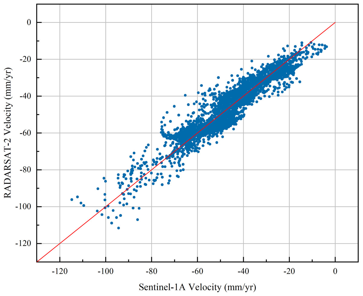
Figure 7: Comparative analysis of deformation correlation at homologous points from multi-source monitoring data.
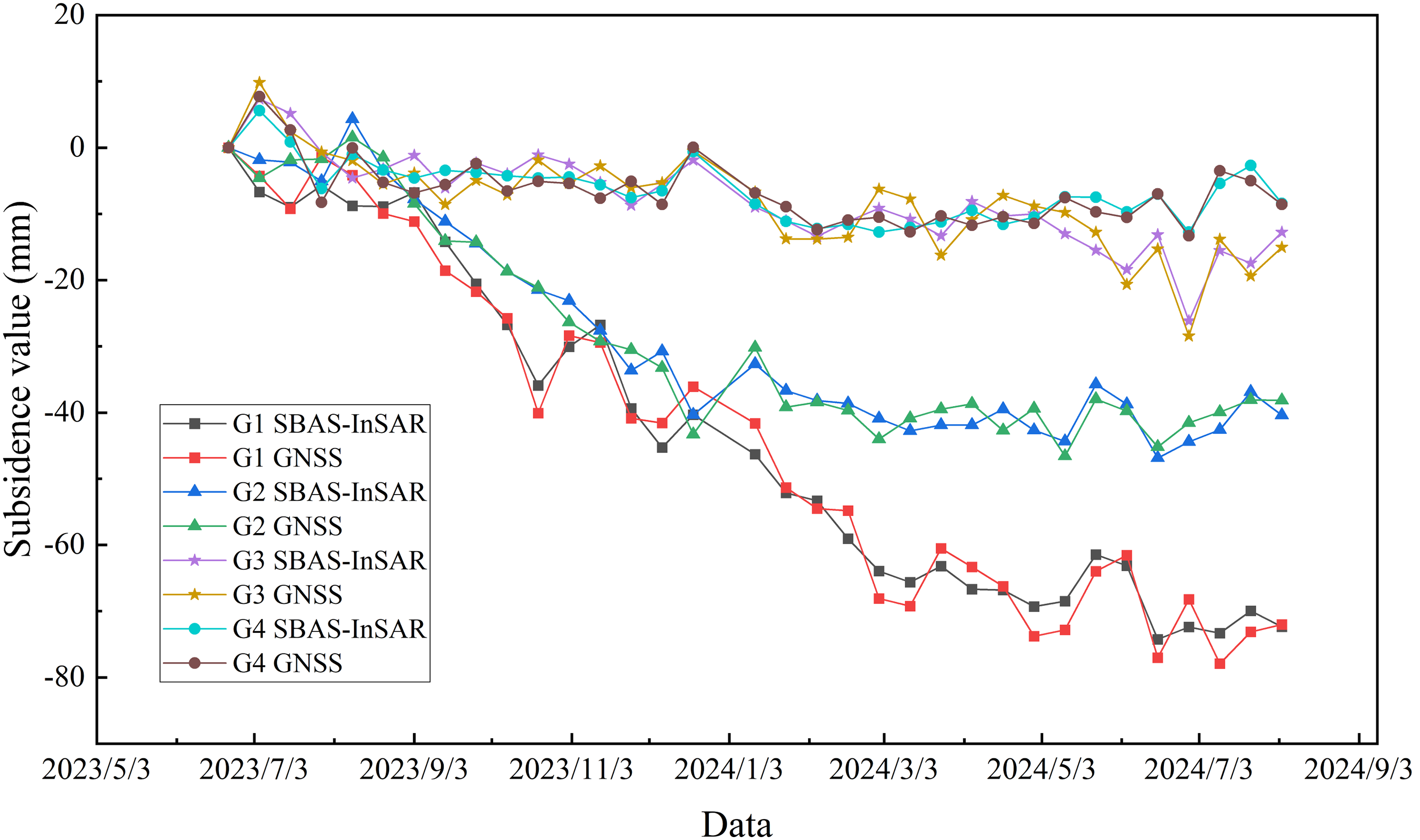
Furthermore, we collected GNSS monitoring data from four stations. These stations were distributed across the subsidence area in the eastern part of the mining area and residential area west of Region B. We compared GNSS-derived cumulative subsidence time series against SBAS-InSAR results. Figure 8 shows the comparisons: The maximum absolute errors between both monitoring results were 4.684, 3.328, 3.194, and 2.462 mm for points G1, G2, G3, and G4, respectively. GNSS and InSAR deformation trends showed good agreement.
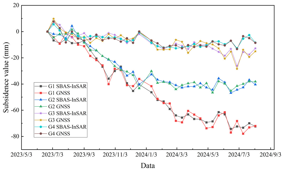
Figure 8: Comparison of SBAS-InSAR and GNSS results.
Both validation approaches confirm SBAS-InSAR result reliability. This technique is suitable for mining subsidence monitoring applications.
Discussion
Characteristics of subsidence basin
To further analyze the deformation characteristics and patterns of the subsidence basin, this study selects Area B as the primary research region. Area B exhibits moderate cumulative subsidence and average subsidence rates. Although Area D shows larger surface subsidence values, mining activities in Area D ceased around March 2024. Within this study’s monitoring period (June 23, 2023 to August 4, 2024), mining only occurred during the first 8 months in Area D. The subsequent 5 months represented a residual subsidence phase. Consequently, Area D provides an insufficiently long effective subsidence time series. Capturing the complete characteristics of surface subsidence during active mining is difficult with such short data.
In contrast, Area B is the core mining area of the Yinying Coal Mine from 2023 to 2025. Area B offers a sufficiently long time series within the monitoring period. Furthermore, the mining advance information for the 150,302 working face within Area B is complete. This complete data enables better comparison with SBAS-InSAR monitoring results. Such comparisons better reflect the relationship between subsidence and mining progress.
Moreover, the subsidence characteristics in Area B closely align with the overall subsidence pattern of the mining region. This alignment effectively represents typical subsidence behavior under standard mining conditions. Selecting Area B for prediction enables a more accurate linkage between mining activity and the subsidence process. It also provides a reliable scenario for validating the prediction model’s practicality. Consequently, results obtained from Area B offer greater reference value for subsidence early warning. Figure 9 illustrates the time-series subsidence plot of this subsidence basin.
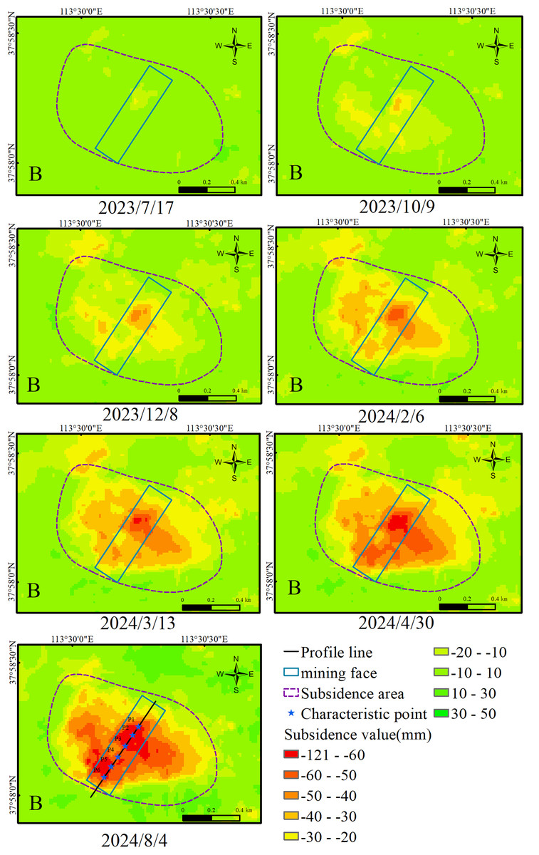
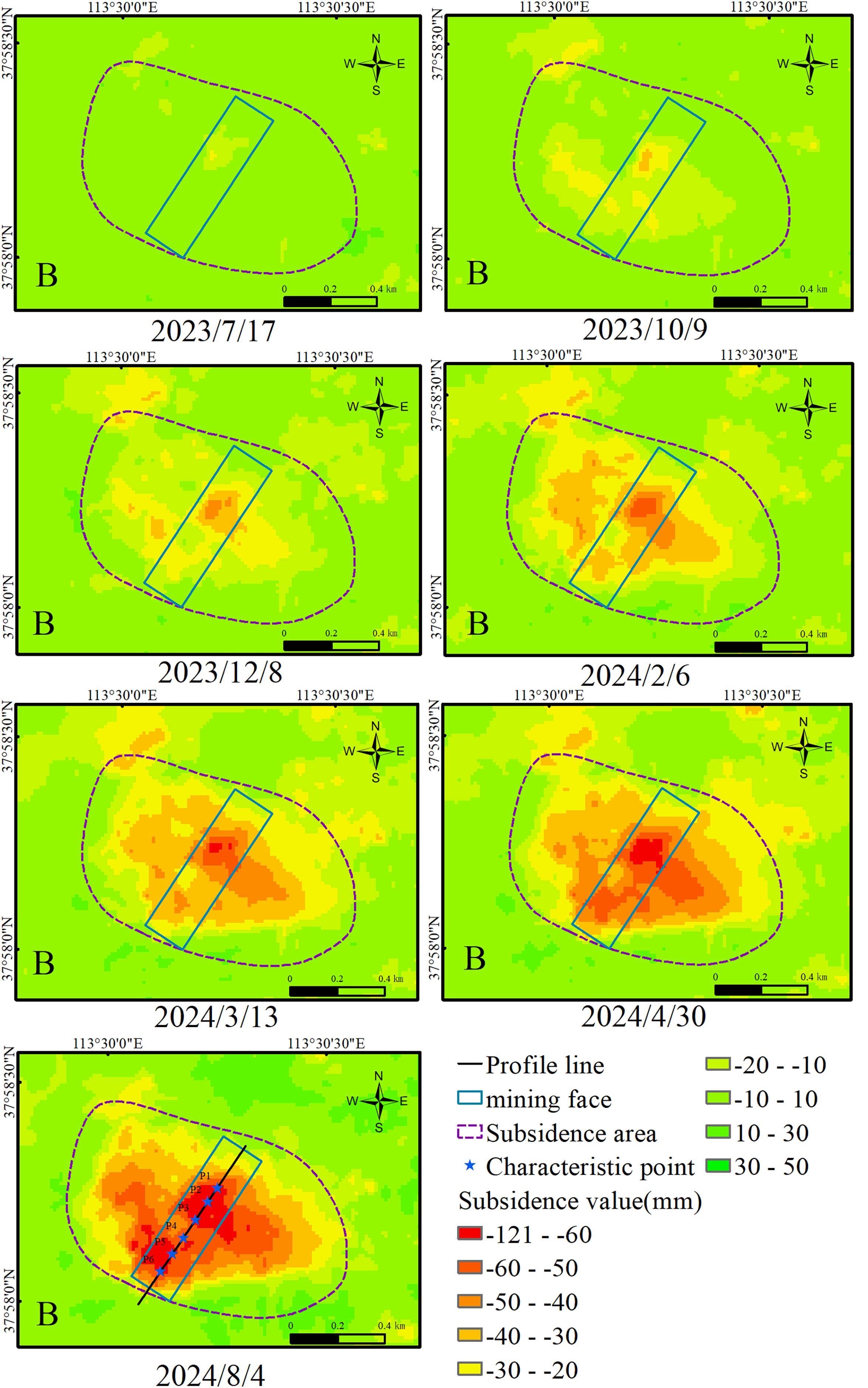
Figure 9: Time-series subsidence plot of subsidence area B.
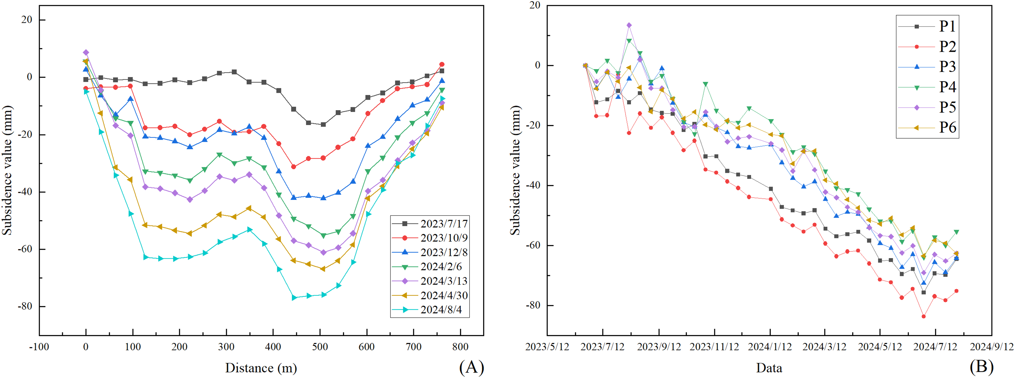
The plot demonstrates progressive expansion of subsidence from northeast to southwest. Subsidence area B exhibits continuous downward movement between June 23, 2023 and August 4, 2024. A profile line is established along the mining face orientation. Twenty-five sampling points are selected at 32-m intervals from southwest to northeast along this profile. The SBAS-InSAR monitoring results provide cumulative subsidence time series at these points. These time-series data generate the temporal cumulative subsidence curve along the profile line. Figure 10A displays the time-series cumulative subsidence curve of the profile line derived from this analysis. Furthermore, six characteristic points (P1–P6) were selected at uniform 75-m intervals along the profile line. These points comprehensively cover the subsidence basin’s gradient zone from the center to the margin. P1 and P2 are located at the subsidence center. This area experiences the maximum mining impact, reflecting core extraction zone deformation. The surface cover consists of open woodland. This cover lacks dense root consolidation, making it highly susceptible to subsidence from coal seam extraction. P3, P4, and P5 lie within the subsidence transition zone. Moderate subsidence here illustrates the subsidence funnel expansion process. The surface cover is shrubland. Dense shrub roots provide topsoil consolidation, mitigating coal mining impacts. P6 is positioned at the subsidence margin. Minor subsidence here reflects indirect mining disturbance. The surface cover is farmland. Loose soil structure and severe erosion make this farmland vulnerable to mining-induced subsidence. These six points form a uniform distribution along the working face’s strike-direction profile line. They collectively represent the subsidence center, transition zone, and margin area. This distribution effectively captures Area B’s subsidence patterns.
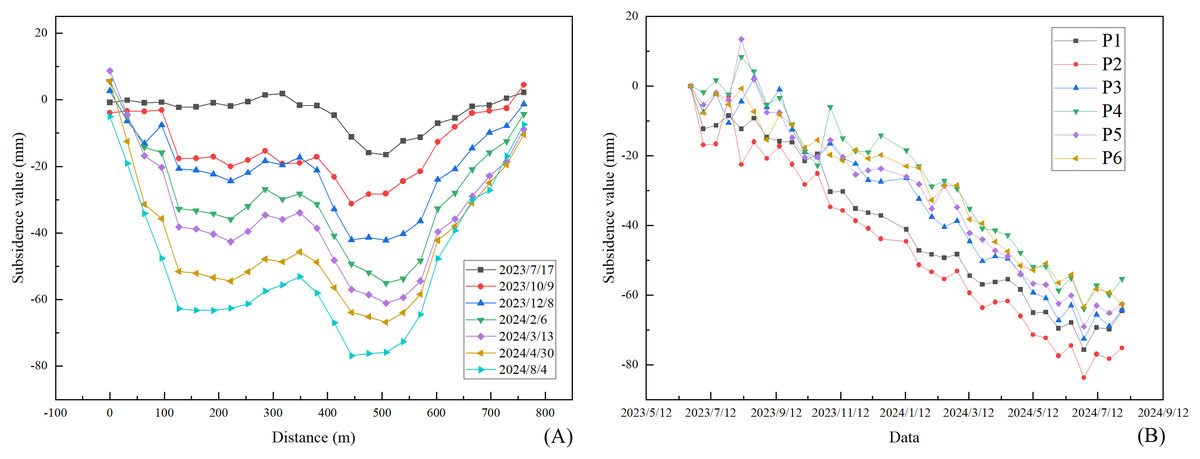
Figure 10: (A) Time-series cumulative subsidence curve of the profile line; (B) Subsidence of the characteristic points with time.
Figures 9 and 10 reveal the evolution of surface subsidence in area B corresponding to the advance of the 150,302 mining face. The mining face advanced from northeast to southwest starting in June 2023. By July 17, 2023, SBAS-InSAR monitoring detected initial subsidence near the northeastern end of the face. This subsidence formed a small funnel-shaped area with a maximum cumulative subsidence of approximately −20 mm. The surface response was initial at this stage due to the short advance distance. Subsequently, the mining face continued advancing. By October 9, 2023, SBAS-InSAR monitoring showed the subsidence area expanding southwestward, covering the extracted portion of the face. The maximum cumulative subsidence increased to −36 mm, and the subsidence funnel elongated along the face strike. Simultaneously, slight subsidence appeared in surrounding areas affected by indirect mining disturbance.
By March 13, 2024, the mining face had advanced to its central section. SBAS-InSAR monitoring indicated continued subsidence across the affected area. The maximum cumulative subsidence reached −63 mm. However, the spatial extent of the subsidence area showed no significant increase compared to February 6, 2024. From March 13, 2024, to August 2024, the mining face advanced further towards the southwestern end. SBAS-InSAR monitoring then showed the subsidence area fully covering the mining face and a surrounding zone within 300 m. The subsidence center moved approximately 80 m southwestward. The average subsidence value of the subsidence center is −78 mm. Subsidence continued within the existing surrounding disturbance zone, but no significant new subsidence areas emerged.
Furthermore, Fig. 10A shows higher subsidence rates occurred in the northeastern part of the face between June 2023 and February 6, 2024. After the mining advance reached the central section on March 13, 2024, the subsidence rate decreased in the northeastern part but increased in the southwestern part. This differential subsidence rate further demonstrates the direct link between surface movement and mining face activity.
In summary, the direction of subsidence area expansion and the migration path of the subsidence center in Area B, monitored by SBAS-InSAR, synchronized precisely with the mining face advance. SBAS-InSAR also clearly captured the subsidence response in areas indirectly disturbed by mining. These observations confirm the spatial and temporal correlation between mining activity and surface deformation.
Bayesian optimization-based hyperparameter tuning
To optimize hyperparameters for Prophet and LSTM models, this study randomly selects 10 high-coherence subsidence points in the study area. SBAS-InSAR-derived time-series subsidence data are acquired for these points. The first 27 steps form the training set, while the last seven steps serve as the testing set. Mean absolute error (MAE) is selected as the evaluation metric for prediction performance.
The parameter search spaces for Prophet and LSTM are defined as specified in Table 2. The Bayesian optimization framework yields the following optimal configurations: Prophet (seasonality prior scale = 0.008, weekly seasonality = True, changepoint prior scale = 0.69, changepoint range = 0.5, seasonality mode = ‘additive’); LSTM (hidden size = 17, time window = 18, num epochs = 61, num layers = 2).
| Prophet | LSTM | ||
|---|---|---|---|
| Parameter name | Search space | Parameter name | Search space |
| seasonality_prior_scale | (0, 1) | hidden_size | (1, 64) |
| weekly_seasonality | (True, False) | time_window | (1, 25) |
| changepoint_prior_scale | (0, 1) | num_epochs | (1, 128) |
| changepoint_range | (0.4, 1) | num_layers | (1, 3) |
| seasonality_mode | (multiplicative, additive) | ||
Model prediction and results analysis
Characteristic point prediction and model performance comparison
This study extracted time-series cumulative subsidence data of six characteristic points in subsidence area B using SBAS-InSAR technology. The first 27 steps of data for each characteristic point served as the training set, and the subsequent seven steps as the validation set. The Prophet model and LSTM model with hyperparameter optimization were employed to predict subsidence for the subsequent 12 steps, The first seven steps of the prediction results were compared with the validation set, while the last five steps were used to demonstrate the future deformation trends. Two accuracy metrics were introduced to evaluate model performance: MAE and root mean square error (RMSE). The formulas are defined as follows:
(10)
(11)
In these formulas, represents measured values, denotes predicted values. Using MAE and RMSE, this study systematically compared the Prophet and LSTM models. The analysis revealed performance differences in subsidence prediction, providing a scientific basis for model selection.
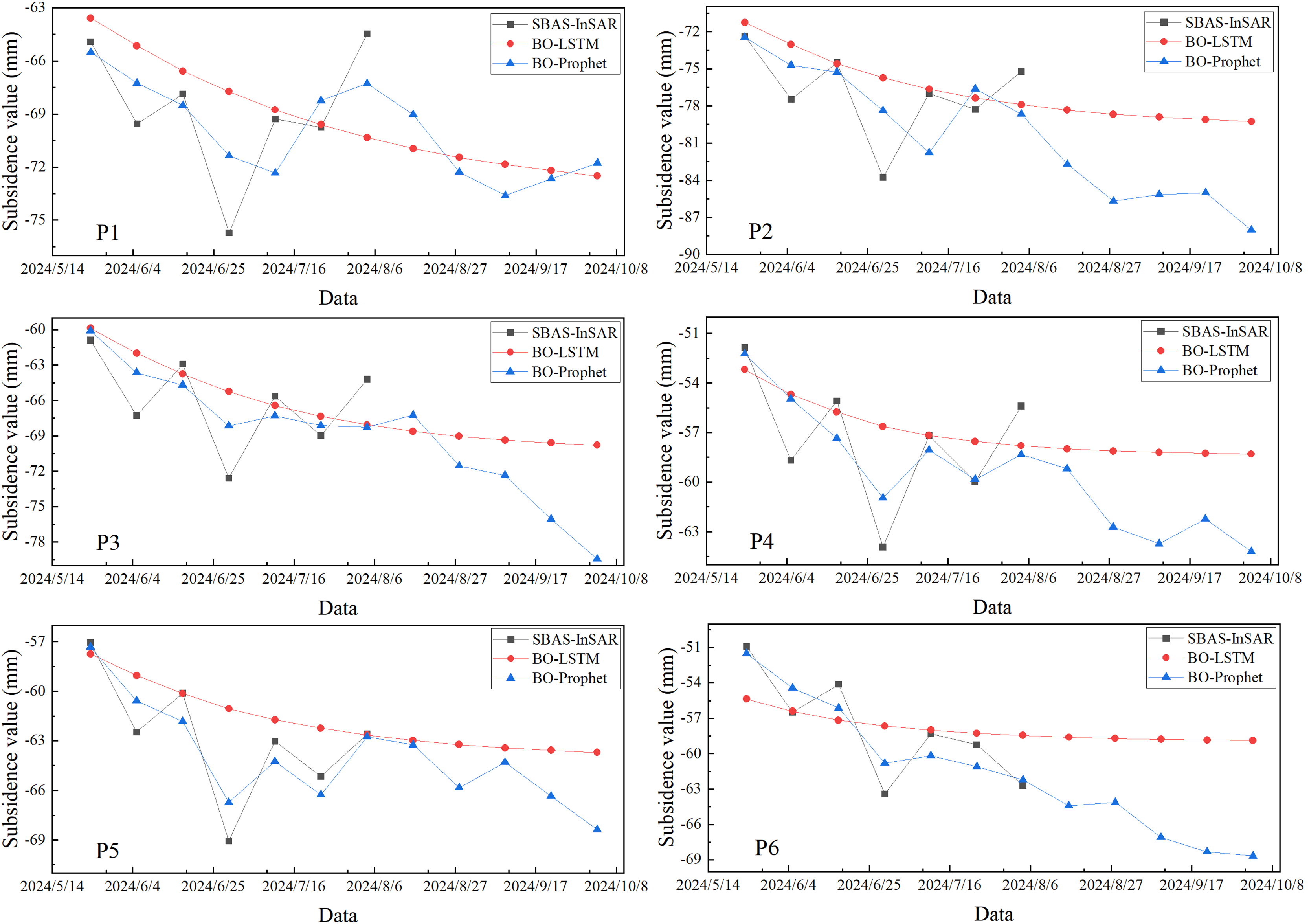
Figure 11 illustrates the comparative performance of the prediction models. The BO-Prophet model exhibits specific error distribution characteristics across seven prediction periods for six characteristic points. The maximum absolute error values for each characteristic point are 4.35, 5.38, 4.45, 3.72, 2.33, and 2.63 mm. Notably, the maximum absolute error for all characteristic points (except P4) concentrates in the third prediction step. This trend aligns with significant subsidence observed in Area B from June 17 to June 29, 2024.
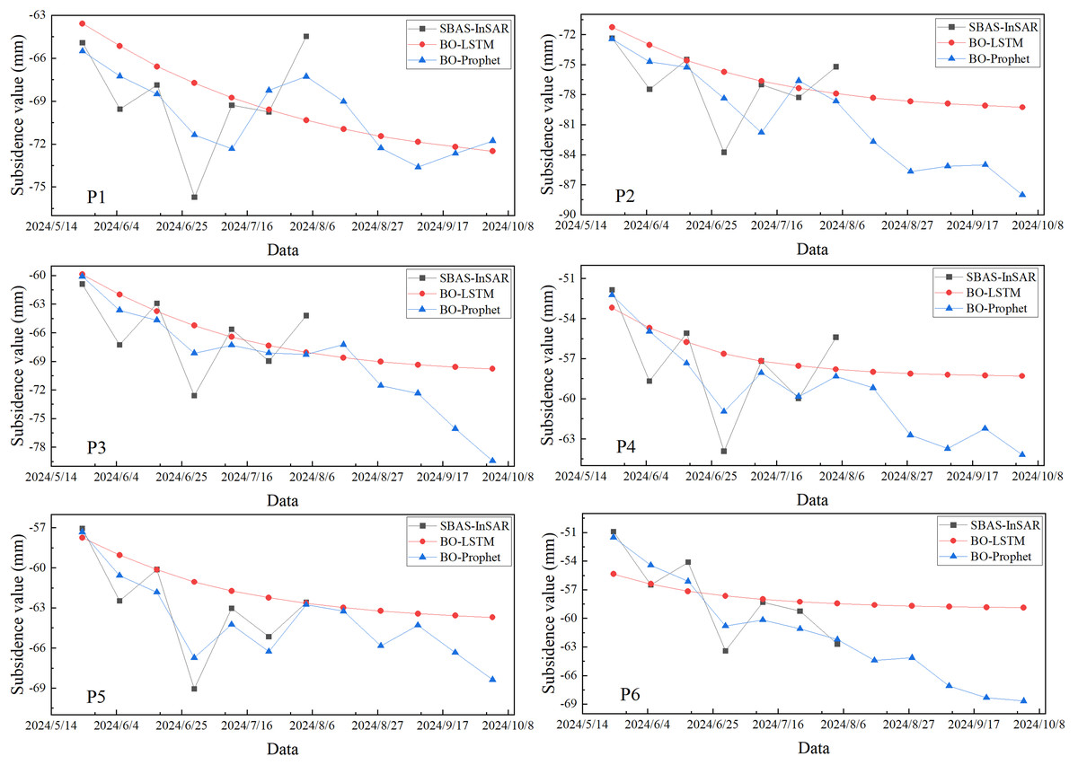
Figure 11: Comparison of prediction results of each prediction model for each characteristic point.
The minimum absolute errors of the BO-Prophet model at six points are 0.59, 0.09, 0.79, 0.15, 0.27, and 0.48 mm. These values confirm high consistency between the BO-Prophet predictions and SBAS-InSAR monitoring data. Visual comparisons demonstrate strong agreement between predicted results and monitoring data.
According to the error indicators presented in Table 3, the BO-Prophet model achieves MAE values of 2.18, 2.69, 2.46, 1.90, 1.25, and 1.63 mm across the six characteristic points. The RMSE values are 2.52, 3.26, 2.85, 2.31, 1.45, and 1.79 mm. Compared to the BO-LSTM model, the BO-Prophet model shows lower errors in both MAE and RMSE. These results validate the higher accuracy and stability of the BO-Prophet model in predicting surface subsidence.
| Point | BO-LSTM | BO-Prophet | ||
|---|---|---|---|---|
| MAE/mm | RMSE/mm | MAE/mm | RMSE/mm | |
| P1 | 3.08 | 4.16 | 2.18 | 2.52 |
| P2 | 2.52 | 3.65 | 2.69 | 3.26 |
| P3 | 2.96 | 3.81 | 2.46 | 2.85 |
| P4 | 2.59 | 3.44 | 1.90 | 2.31 |
| P5 | 2.34 | 3.52 | 1.25 | 1.45 |
| P6 | 2.69 | 3.41 | 1.63 | 1.79 |
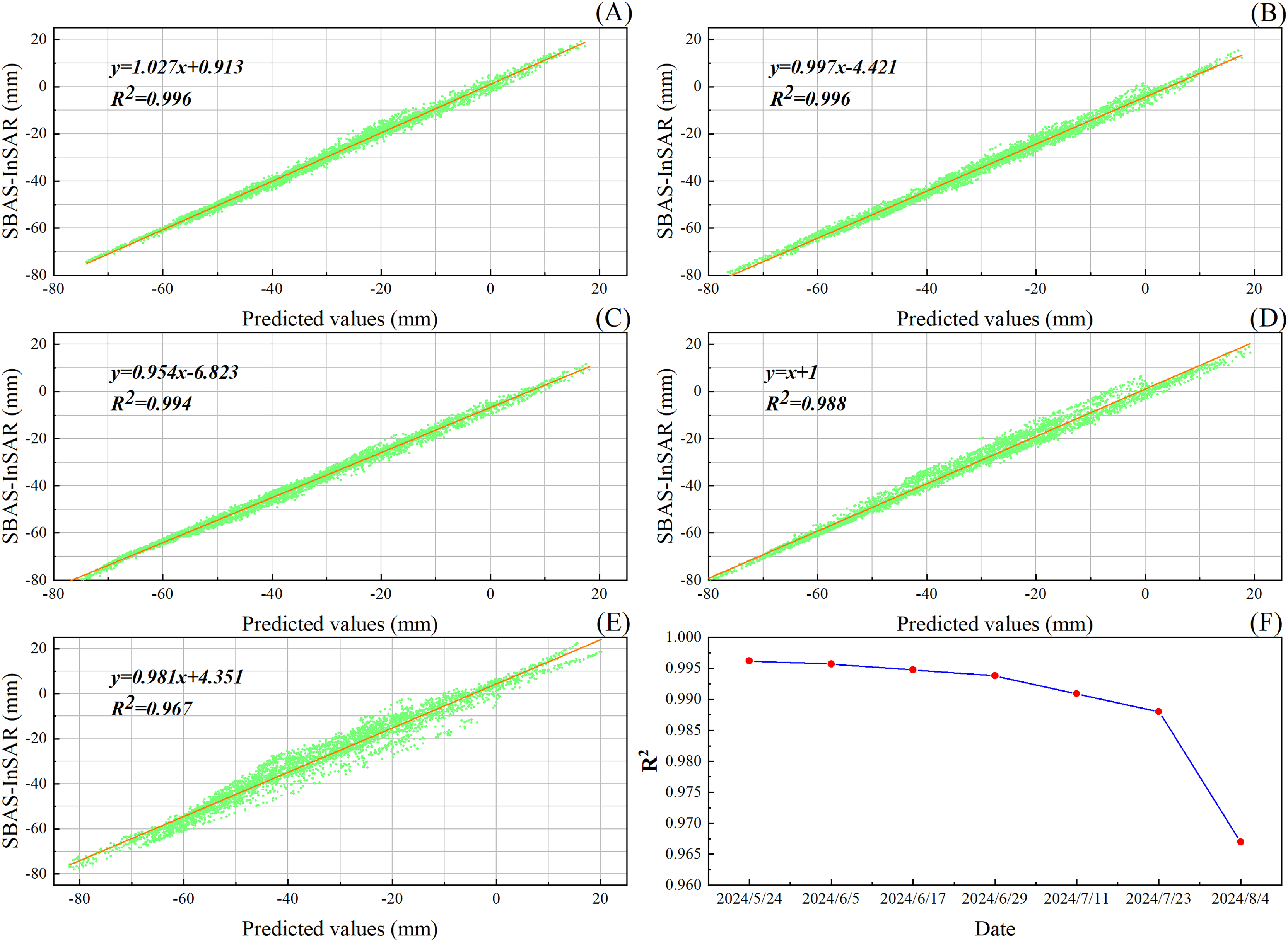
To comprehensively assess prediction accuracy, the BO-Prophet model generated subsidence forecasts across area B. These predictions were compared with SBAS-InSAR measurements through correlation analysis. Figure 12 demonstrates strong consistency between predicted values and SBAS-InSAR values across multiple time spans (12d, 24d, 48d, 72d, 84d). All correlation coefficients exceed 0.96, confirming the model’s effectiveness in large-scale subsidence prediction. Further analysis examines correlation coefficient variations under different time spans. As shown in Fig. 12F, the coefficients gradually decrease over time. This trend indicates diminishing prediction accuracy with increasing forecast duration.
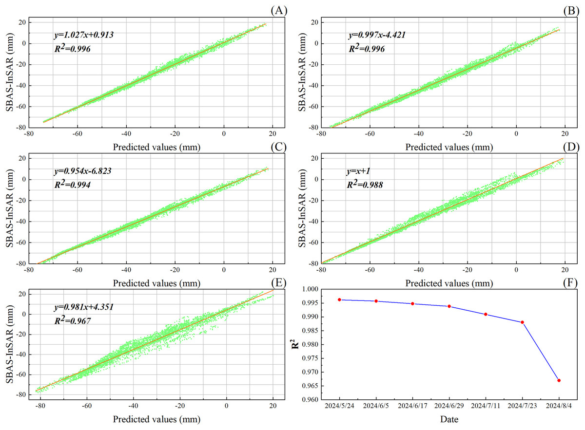
Figure 12: Correlation analysis between SBAS InSAR and prediction results: (A) 12d; (B) 24d; (C) 48d; (D) 72d; (E) 84d; (F) R2 changes over different time spans.
Distribution of errors
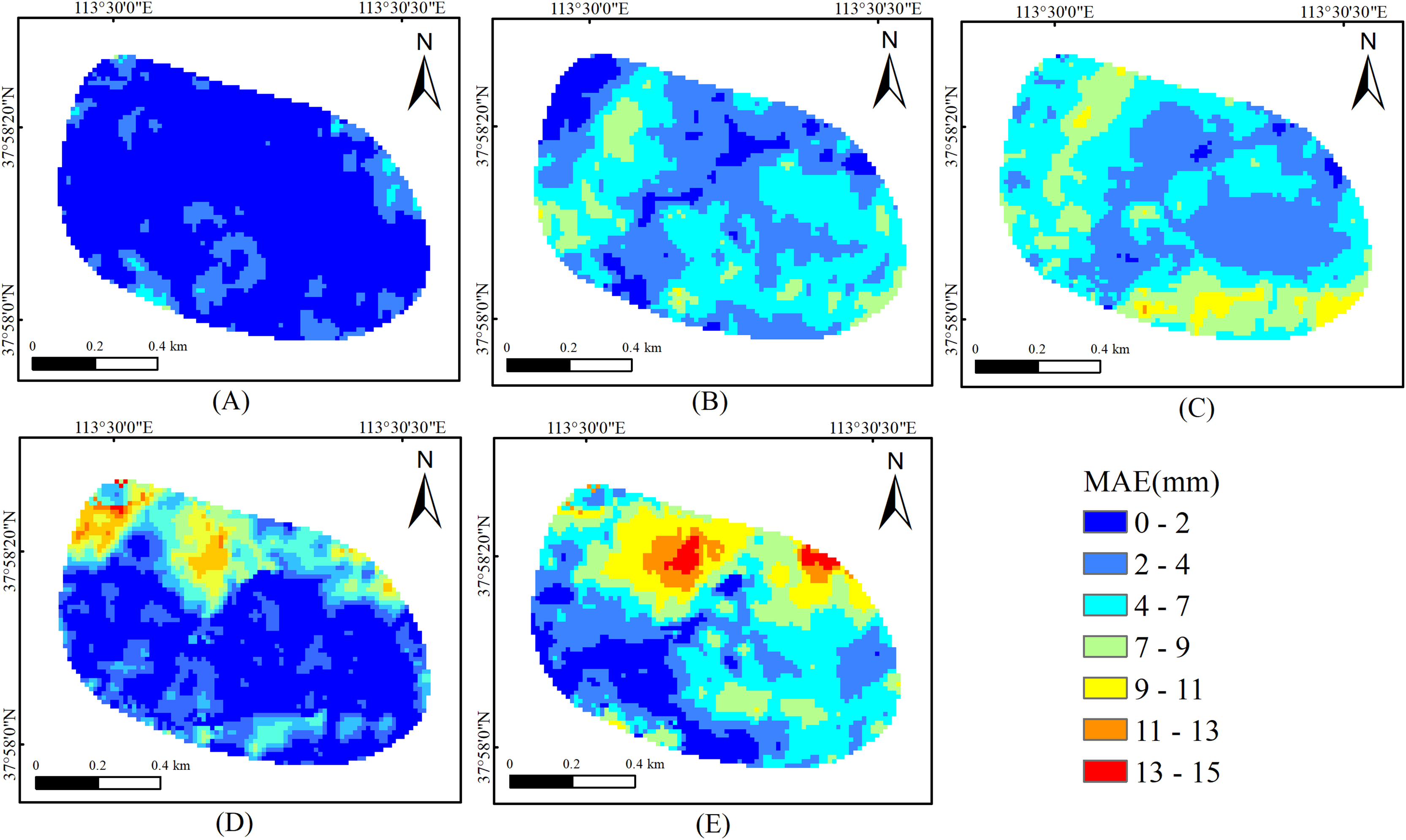
The study investigates spatial error patterns by overlaying BO-Prophet predictions with SBAS-InSAR measurements in area B. This process absolute error distribution map. Figure 13 reveals two critical trends. First, prediction errors progressively increase over time. Second, errors predominantly cluster in the northwestern sector of area B. This area corresponds to the marginal slow subsidence zone of the depression basin. These findings demonstrate BO-Prophet’s superior short-term forecasting capability. However, error accumulation becomes evident with extended prediction horizons. The spatial error concentration suggests systematic biases in specific geological subregions.
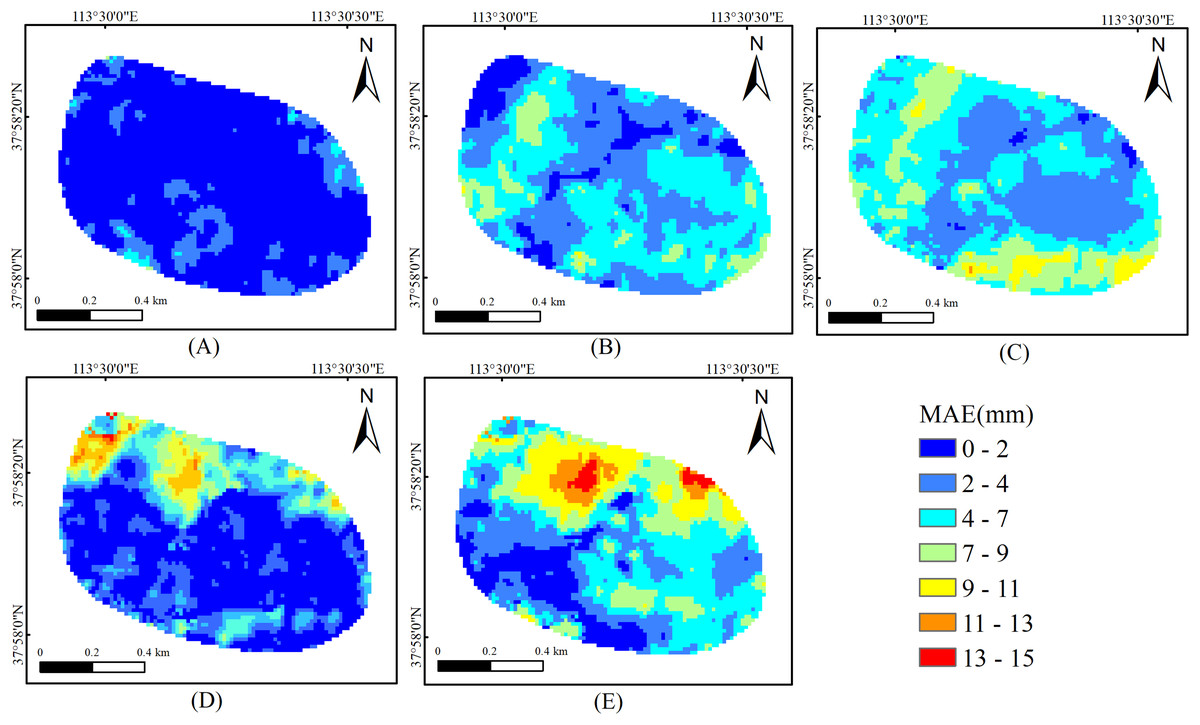
Figure 13: The spatial distribution map of prediction errors in area B. (A) 12d; (B) 24d; (C) 48d; (D) 72d; (E) 84d.
Conclusions
This study focused on the Yinying Coal Mine, utilizing SBAS-InSAR technology to obtain the annual average subsidence rate results and the time-series cumulative subsidence results of Yinying Coal Mine. Then, the study applied the BO-LSTM and BO-Prophet prediction models to forecast subsidence in the mining area, with each model implemented independently for comparative analysis. Key findings are summarized below:
-
(1)
SBAS-InSAR monitoring results: The SBAS-InSAR monitoring results revealed an annual average subsidence rate of up to 115 mm/yr and a maximum cumulative subsidence of 121 mm between June 23, 2023, and August 2, 2024. Both values fell within normal ranges for mining-induced subsidence.
-
(2)
Validation using multi-track data and GNSS: The reliability of SBAS-InSAR results was validated through independent processing of multi-track datasets (ascending and descending tracks) and comparison with GNSS measurements. A Pearson correlation coefficient of 0.946 confirmed high consistency between ascending and descending datasets. Comparisons with four GNSS stations showed maximum absolute errors of 4.684, 3.328, 3.194, and 2.462 mm, with good agreement in deformation trends.
-
(3)
Spatial analysis of subsidence area B: Longitudinal profile analysis of Subsidence area B showed continuous growth in subsidence over time. The deformation exhibited a distinct funnel-shaped pattern, aligning with typical mining-induced subsidence characteristics.
-
(4)
A comparative analysis evaluates two prediction models using standard performance metrics. The BO-Prophet (MAE = 2.02 mm, RMSE = 2.36 mm) demonstrates superior prediction accuracy over the BO-LSTM (MAE = 2.70 mm, RMSE = 3.67 mm). Further examination confirms high consistency (R2 > 0.96) between BO-Prophet predictions and SBAS-InSAR monitoring results; BO-Prophet has a better prediction effect in short-term predictions. This integration enables effective monitoring and forecasting of mining-induced subsidence. Implementing BO-Prophet with SBAS-InSAR technology enhances early warning systems for mining hazards. It supports disaster prevention and mitigation strategies in mining areas.
Future studies will focus on enhancing the model’s robustness, generalizability, and rigor through integrated efforts. We will expand cross-site validation in diverse mining areas—including other Loess Plateau regions, high-steep mountain zones, and major coal-producing regions in Shanxi, Shaanxi, and Inner Mongolia—to verify its applicability beyond Yinying. We will also compare Bayesian optimization with alternatives (e.g., genetic algorithms) to identify the most robust hyperparameter tuning strategy for varied scenarios. Additionally, we will strengthen multi-source validation by optimizing GNSS deployment and integrating supplementary ground data (leveling, uncrewed aerial vehicle (UAV) photogrammetry) to boost reliability of both monitoring and prediction. Finally, we will advance the framework with physics-constrained deep learning and spatiotemporal attention mechanisms to address long-term error accumulation and sensitivity to geological heterogeneities. These efforts will refine early warning capabilities, support data-driven disaster prevention, and promote sustainable mining practices.
Supplemental Information
Code.
Code and data used in the article. Among them, prophet_beys.py is used for Bayesian optimization of Prophet model hyperparameters, lstm_beys.py for Bayesian optimization of LSTM model hyperparameters, and predic.py for temporal subsidence prediction. Within the “dataset” folder, point.csv contains the cumulative subsidence time-series data of Area B, and 10point.csv contains the cumulative subsidence time-series data of selected points for model Bayesian optimization.
The TIFF files used in the study.
Main raster data files (.tif), supporting geographic reference files (.tfw), and pyramid files (.ovr) for GIS mapping. Specifically, figure6.tif records the annual average deformation rate of the study area; figure9 (1)–(7).tif respectively record the cumulative subsidence values of Area B on July 17, 2023, October 9, 2023, December 8, 2023, February 6, 2024, March 13, 2024, April 30, 2024, and August 4, 2024; and figure13 (1)–(5).tif respectively record the absolute error distributions of 12-day, 24-day, 48-day, 72-day, and 84-day subsidence predictions for Area B. The .tfw files are geographic reference files matching each .tif, while the .ovr files are multi-resolution thumbnail pyramid files (for accelerated display); all three types of files must be loaded together in GIS software for use.
Comparative analysis of deformation correlation at homologous points from Multi-Source Monitoring Data.
Used for creating Figure 7 in the article, this file contains the data processing results of Sentinel-1A and RADARSAT-2 satellites.
Time-series cumulative subsidence of the profile line.
Used for creating Figure 10 in the article, this file contains the time-series cumulative subsidence curve data of the profile line in Area B.
Subsidence of the points with time.
Used for creating Figure 10 in the article, this file contains the cumulative subsidence time-series data of 6 feature points in Area B.
Comparison of prediction results of each prediction model for each characteristic point.
Used for creating Figure 11 in the article, this file contains the subsidence prediction results of 6 feature points in Area B.
Correlation analysis between SBAS InSAR and prediction results (time span 12d).
Used for creating Figure 12A in the article, this file contains the results of 12-day subsidence prediction for Area B.
Correlation analysis between SBAS InSAR and prediction results (time span 24d).
Used for creating Figure 12B in the article, this file contains the results of 24-day subsidence prediction for Area B.
Correlation analysis between SBAS InSAR and prediction results (time span 48d).
Used for creating Figure 12C in the article, this file contains the results of 48-day subsidence prediction for Area B.
Correlation analysis between SBAS InSAR and prediction results (time span 72d).
Used for creating Figure 12D in the article, this file contains the results of 72-day subsidence prediction for Area B.
Correlation analysis between SBAS InSAR and prediction results (time span 84d).
Used for creating Figure 12E in the article, this file contains the results of 84-day subsidence prediction for Area B.
R2 changes over different time spans.
Used for creating Figure 12F in the article, this file contains the R² values between the subsidence prediction results and SBAS-InSAR monitoring values.