
A hybrid fusion of the recurrent neural network and bidirectional long short-term memory for wind speed prediction in the South China Sea
- Published
- Accepted
- Received
- Academic Editor
- Giovanni Angiulli
- Subject Areas
- Artificial Intelligence, Data Mining and Machine Learning, Data Science, Scientific Computing and Simulation, Theory and Formal Methods
- Keywords
- Deep learning, Machine learning, Wind speed prediction, Bidirectional long short term memory, Recurrent neural network, South China Sea
- Copyright
- © 2025 Mojahid et al.
- Licence
- This is an open access article distributed under the terms of the Creative Commons Attribution License, which permits unrestricted use, distribution, reproduction and adaptation in any medium and for any purpose provided that it is properly attributed. For attribution, the original author(s), title, publication source (PeerJ Computer Science) and either DOI or URL of the article must be cited.
- Cite this article
- 2025. A hybrid fusion of the recurrent neural network and bidirectional long short-term memory for wind speed prediction in the South China Sea. PeerJ Computer Science 11:e3303 https://doi.org/10.7717/peerj-cs.3303
Abstract
Wind speed prediction in the South China Sea is crucial for enhancing maritime safety, supporting operational planning, and optimizing economic activities in sectors such as offshore energy, shipping, and disaster preparedness. In recent years, the statistical auto-regressive integrated moving average (ARIMA) model and advanced deep learning models such as recurrent neural networks (RNN), long short-term memory (LSTM) networks, and Bidirectional LSTM (BiLSTM) have shown strong potential for time series forecasting due to their capacity to model temporal dependencies. However, these models often face limitations in simultaneously capturing rapid short-term fluctuations and long-term temporal patterns in meteorological data. To address this challenge, we propose a novel hybrid architecture, h-RNN-BiLSTM, which integrates the short-term dynamic modeling capability of RNN with the long-range bidirectional dependency modeling of BiLSTM. This fusion enables multi-scale temporal pattern learning, thereby improving forecasting accuracy. The model is evaluated using two widely recognized spatiotemporal datasets: the European Centre for Medium-Range Weather Forecasts (ECMWF) and the Global Forecast System (GFS). Data preprocessing, including missing value imputation and standardization, was applied to ensure data consistency and improve model convergence. Experiments were conducted in two settings: (i) short-term datasets from GFS and ECMWF, and (ii) long-term ECMWF datasets. The performance of h-RNN-BiLSTM was compared against baseline RNN, LSTM, BiLSTM, and the ARIMA model using root mean square error (RMSE) and mean absolute percentage error (MAPE) as evaluation metrics. Results demonstrate that the proposed model consistently outperforms the deep learning baselines and ARIMA, with the most significant gains observed for the long-term ECMWF dataset. Specifically, the model reduced error by 99.7% compared with ARIMA, 70.3% compared with RNN, 30.7% compared with LSTM, and 37.6% compared with BiLSTM. For MAPE, the improvements were 84.3% over ARIMA, 38.8% over RNN, 40.3% over LSTM, and 32.1% over BiLSTM. To the best of our knowledge, this is the first study to integrate RNN and BiLSTM for multi-scale wind speed prediction in the South China Sea, demonstrating improved predictive accuracy over both deep learning and statistical baselines. These findings highlight the model’s operational potential for energy planning, navigation safety, and weather risk management.
Introduction
Wind speed is a crucial factor in meteorology, with significant implications for logistics, renewable energy generation, aviation, and coastal operations (Nasir et al., 2023). Its importance lies in shaping weather patterns and influencing environmental conditions (Liu et al., 2022). Excessive wind speeds can pose severe hazards, particularly in coastal regions, leading to catastrophic events such as hurricanes and cyclones that threaten both human life and infrastructure. Accurate prediction of wind speed is therefore essential, as it informs decision-making and supports the development of adaptive strategies for managing environmental risks. The South China Sea (SCS), recognized as a promising site for floating wind farms, offers abundant wind resources, frequent high-speed winds, and stable wind power density (Nasir et al., 2023). Reliable wind speed forecasts are especially valuable for the offshore wind energy industry, as they guide turbine placement, support energy production planning, and ensure operational safety while mitigating risks from extreme weather events. Thus, accurate wind speed forecasting in the SCS is critical for optimizing resource management, enhancing safety, and promoting economic resilience across multiple sectors.
A wide range of approaches including physical (numerical), statistical, and deep learning methods have been applied to the challenging task of wind speed forecasting. Numerical weather prediction (NWP) methods, based on complex physical equations, provide highly detailed simulations but demand substantial computational resources and long processing times (Samad et al., 2020). Statistical methods such as the autoregressive integrated moving average (ARIMA) and its variants have been widely applied in wind speed forecasting due to their demonstrated effectiveness (Soman et al., 2010; Jung & Broadwater, 2014; Li et al., 2018; Aasim & Mohapatra, 2019; Kushwah & Wadhvani, 2025; Taoussi, Boudia & Mazouni, 2025). However, ARIMA is generally more effective for linear time series than for nonlinear ones (Qin, Li & Du, 2017). The inherently stochastic and nonlinear characteristics of wind speed highlight the limitations of these statistical methods in capturing complex dynamics.
Recently, deep learning has been used in the time series prediction to effectively handle the unpredictability and instability of wind speed sequences. This approach facilitates enhanced performance by directly extracting optimal features from raw time-series data (Khodayar, Kaynak & Khodayar, 2017). The deep learning approaches are known for their relatively simple implementation and low computing requirements (Salman et al., 2018). The models mostly consist of neural networks with intricate hidden layer architectures (Aly, 2020). Neural networks such as artificial neural networks (ANN) and recurrent neural networks (RNN) are commonly used for wind speed forecasting due to their capacity to capture nonlinear input–output relationships (Zhu et al., 2018; Cali & Sharma, 2019; Marndi, Patra & Gouda, 2020). RNN is a type of neural network specifically designed to analyze time-series data and make predictions based on a given set of intervals (Khodayar, Kaynak & Khodayar, 2017). In the literature, researchers have utilized RNN based models for the purpose of wind speed prediction (Liu, Mi & Li, 2018; Duan et al., 2021; Khan et al., 2024; Kacimi et al., 2025). This network has the ability to accept information from a previous state and store it in the hidden layer, which can then be accessed in the current state. Thus, this network is well-suited for forecasting wind speed using historical time series data (Gonzalez & Yu, 2018; Liu et al., 2020). A comparative study of three learning models, namely support vector machine, ANN, and RNN for weather prediction revealed that RNN yielded the most optimal outcomes (Singh et al., 2019). Nevertheless, while RNNs excel at forecasting short-term weather patterns, they may have difficulties in capturing long-term relationships because of the vanishing gradient problem.
Another often-used deep learning approach for creating predictions based on time-series data is the long short-term memory (LSTM) network (Ibrahim et al., 2020). The LSTM model, as presented by Shi et al. (2015) is an enhanced version of the ANN model that successfully addresses the issue of vanishing gradients in RNNs. This is achieved by incorporating cell state and gates to regulate the flow of information. The model is versatile and may be used in various types of situations, as mentioned by Nasser, Rashad & Hussein (2020). An important benefit of LSTM is its ability to retain knowledge over extended periods, enabling it to effectively address long-range dependence issues (Zhang et al., 2017; Liang, Nguyen & Jin, 2018; Puspita Sari et al., 2021; Kannan, Subbaram & Faiyazuddin, 2023). Research has shown that LSTM achieves better predictive accuracy than the feed forward approach for wind speed forecasting in the Indian Ocean (Biswas & Sinha, 2021). In one separate investigation, Hossain et al. (2015) implemented a deep neural network with an auto-encoder in predicting meteorological conditions in Nevada. Meanwhile, a variant of LSTM was proposed by Sun et al. (2023) in predicting short term wind speed in the SCS region. A deep learning multi-stacked architecture based on LSTM was also suggested by Akram & El (2016), which can predict meteorological characteristics such as temperature, wind speed, and humidity. However, due to its limitation in encoding bidirectional information, LSTM can only consider one side of a time-series connection. To overcome this problem, Graves & Schmidhuber (2005) introduced the Bidirectional LSTM (BiLSTM) neural network, which has two LSTM layers. In this state-of-the-art deep learning model, the input data is processed in both forward and backward directions, leading to more accurate predictions. The BiLSTM model and its variants models have demonstrated good performance in several meteorology prediction tasks, including wind speed prediction (Biswas & Sinha, 2021; Liu, Shu & Chan, 2025), wave height prediction (Wang et al., 2022), wind power prediction (Ma & Mei, 2022; Wan et al., 2024), wave energy prediction (Song et al., 2023) and weather prediction (Zhang et al., 2024). While BiLSTM effectively handles long-range dependencies, it is less sensitive to rapid short-term fluctuations compared to RNN.
It is important to note that wind speed characteristics vary significantly across different geographic regions, implying that a single predictive model may not yield optimal accuracy in all locations for ensuring operational safety and building resilience against the potential negative impacts of strong winds (Liu & Chen, 2019; Lau et al., 2022). In addition to geographical factors, the choice of dataset used for forecasting also plays a crucial role in determining prediction accuracy. Among the most widely used datasets in weather forecasting research are the European Centre for Medium-Range Weather Forecasts (ECMWF) dataset (ECMWF, 2023) sourced from https://www.ecmwf.int/en/forecasts/datasets and the Global Forecast System (GFS) dataset (GFS, 2023) sourced from https://www.ncei.noaa.gov/products/weather-climate-models/global-forecast both of which are publicly available and provide multivariate, time-sequenced weather parameters. These datasets exhibit complex temporal patterns that require models capable of capturing both short-term variations and long-term dependencies. Consequently, there is an urgent need for deep learning models that can effectively address these dynamics.
In contrast to the studies reviewed earlier, which typically rely on statistical methods or a single deep learning framework such as RNN, LSTM, or BiLSTM, this study proposes a hybrid RNN-BiLSTM model (h-RNN-BiLSTM). By integrating RNN and BiLSTM architectures, the h-RNN-BiLSTM model complements the strengths of both approaches and is specifically tailored for wind speed forecasting in the SCS. Moreover, most studies are limited to a single dataset or geographic context, whereas this study employs both ECMWF and GFS datasets to comprehensively evaluate short-term and long-term forecasting performance. By doing so, the proposed approach addresses the unique meteorological dynamics of the SCS; a region underexplored despite its strategic importance for offshore wind energy. It also demonstrates the benefits of dataset diversity in enhancing model generalization. To the best of our knowledge, no prior work has developed or tested a hybrid RNN-BiLSTM model for wind speed forecasting in this region, making this study a distinctive contribution that bridges methodological innovation with regional applicability. The key contributions of the article are the following:
A new hybrid deep learning model (h-RNN-BiLSTM) is proposed to forecast wind speed in the SCS region, integrating RNN and BiLSTM architectures for enhanced multi-scale temporal pattern learning.
Two meteorological datasets, ECMWF and GFS are employed to evaluate model performance in short-term (GFS and ECMWF) and long-term (ECMWF) forecasting scenarios.
The proposed model is compared to the well-known statistical method, ARIMA, and the state-of-the-art deep learning models which are RNN, LSTM and BiLSTM models.
The manuscript’s structural framework is presented in the following manner: ‘Materials and Methods’ outlines the materials and methods employed in this study. ‘Results’ provides experimental results, while ‘Discussion’ offers a detailed discussion of those results. ‘Conclusion’ serves as a summary of the final insights obtained from the study’s findings.
Materials and Methods
The methodology employed in this study comprises several key steps: data collection, data preprocessing, model development, model training and testing, and performance evaluation of the forecasting results. The overall workflow is illustrated in Fig. 1, which presents the overall framework of the study.
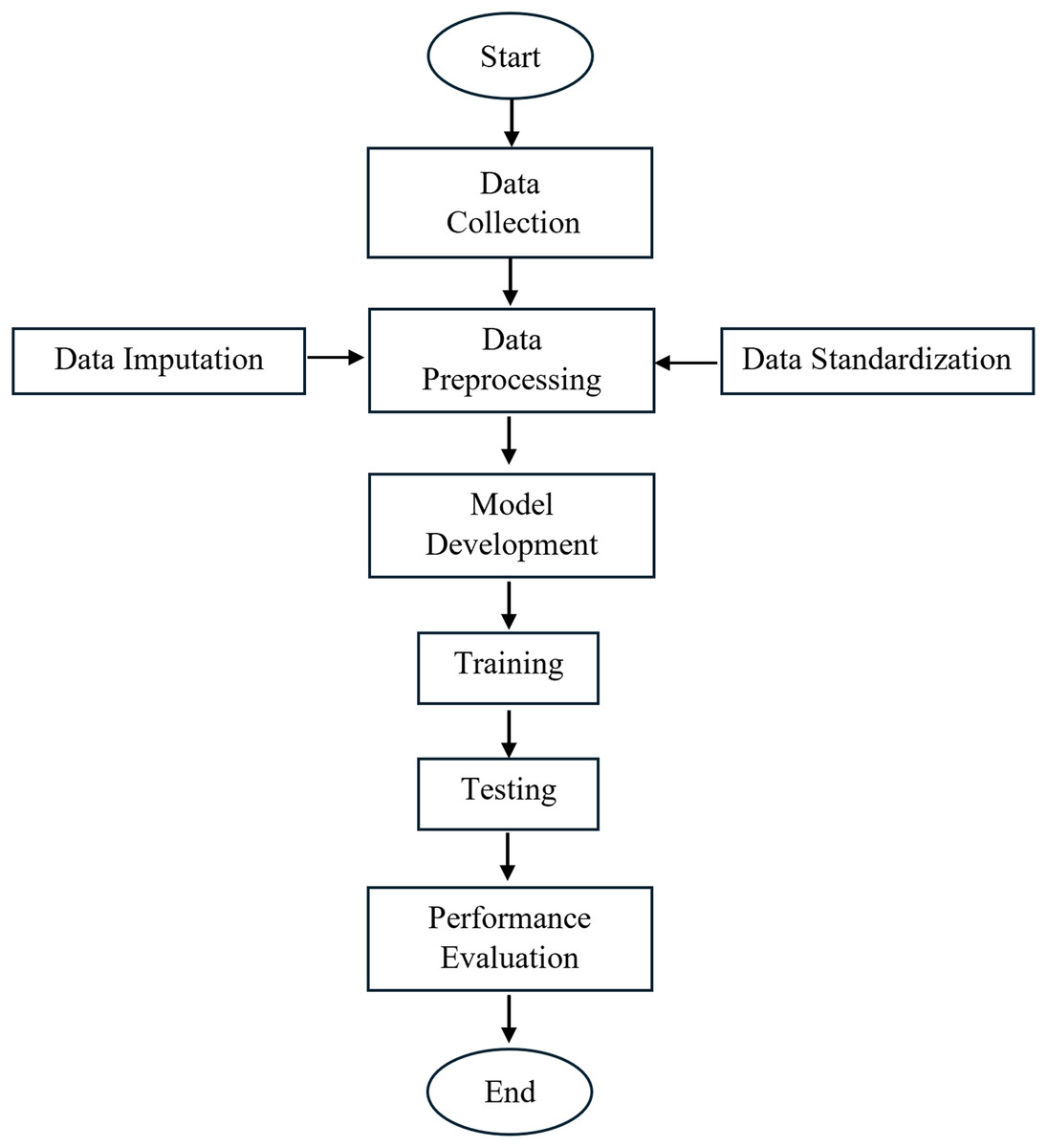
Figure 1: Framework of research methodology.
Data collection
Spatial-temporal weather data over the SCS were obtained from ECMWF and GFS. At the time of this study, the GFS dataset was publicly available only from 00:00:00 on December 2, 2022, to 18:00:00 on May 31, 2023. To enable direct comparison, the ECMWF dataset was restricted to the same period. For extended experimentation, a longer ECMWF dataset covering the period from 00:00:00 on January 1, 2019, to 21:00:00 on August 31, 2023, was also utilized. Accordingly, two groups of datasets were defined: (i) short-term datasets (December 2, 2022–May 31, 2023, from both GFS and ECMWF), and (ii) long-term datasets (January 1, 2019–August 31, 2023, from ECMWF). All datasets were collected at a temporal resolution of 3-h intervals (timestamps). The weather data (parameters) which serve as crucial features in our forecasting model that contribute vital information to predict the target variable (wind speed) are longitude, latitude, sea surface temperature (SST), maximum 2m temperature (t2m), mean sea level pressure (msl), mean total precipitation rate (mtpr), and the 10m u and v direction components of wind. All parameters collectively capture the multidimensional aspects of the atmospheric conditions over the SCS. Analyzing these parameters enables a comprehensive understanding of the complex interactions influencing wind speed dynamics in the SCS region.
Data preprocessing
The GFS dataset contained no missing values, whereas the ECMWF dataset exhibited missing entries for the SST parameter, as illustrated in Fig. 2.
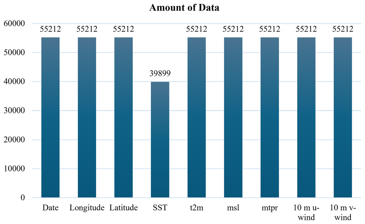
Figure 2: Missing values of sea surface temperature (SST) in the ECMWF dataset.
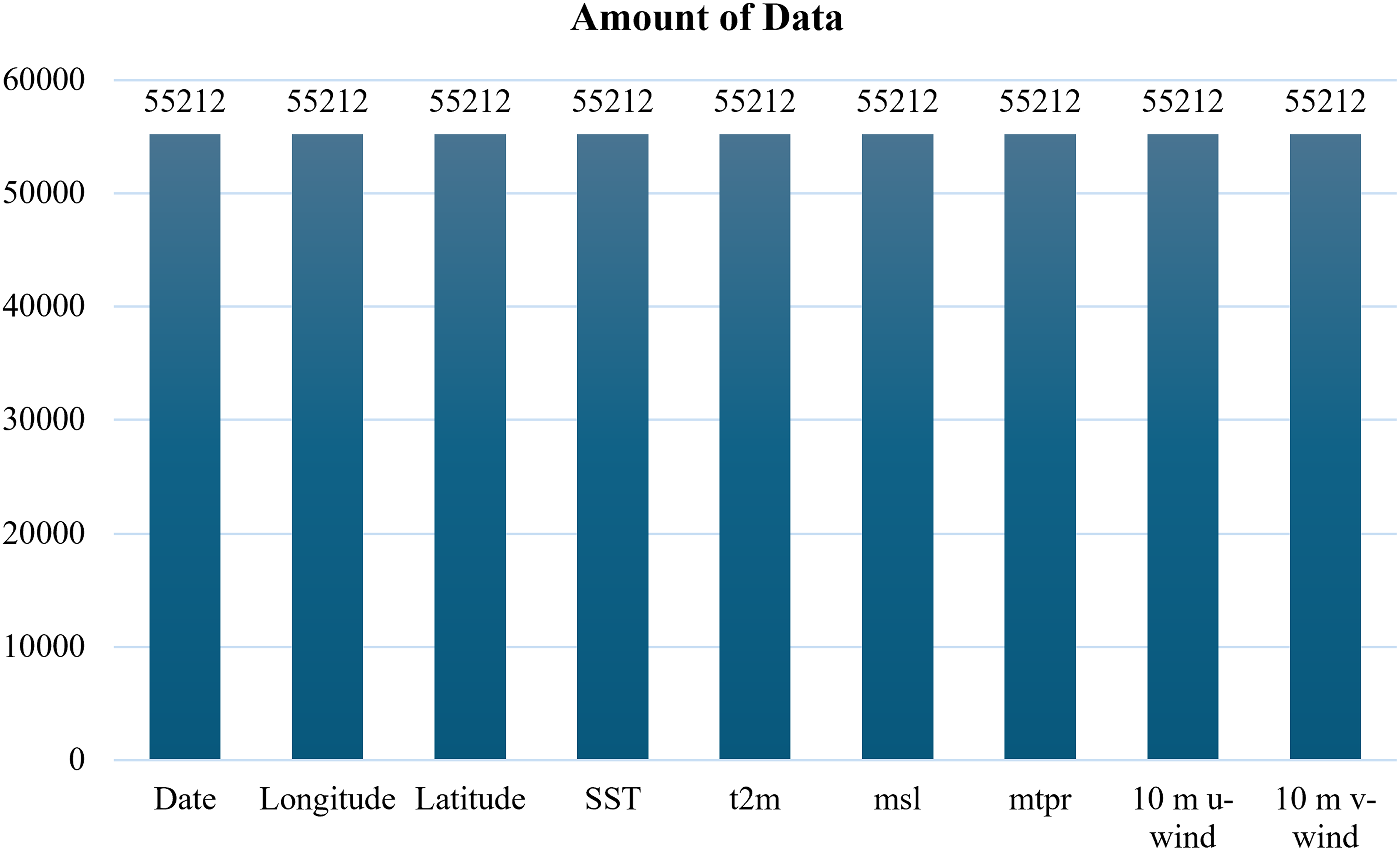
Based on Fig. 2, the bar chart shows the amount of data available for each parameter, highlighting the presence of missing values in SST. To address this issue, mean imputation was applied to the SST column, thereby producing a complete dataset for model training as demonstrated in Fig. 3. Although more sophisticated methods exist, mean imputation was chosen due to the relatively low proportion of missing entries and to maintain computational efficiency for large-scale time series.
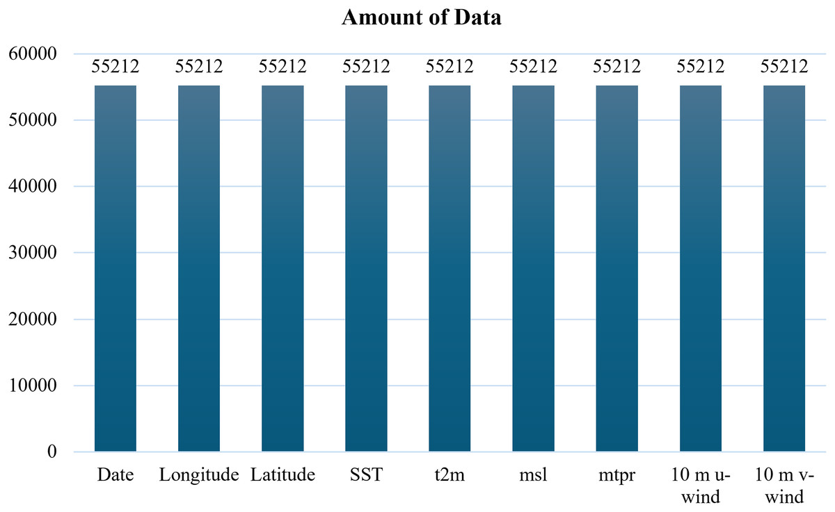
Figure 3: ECMWF dataset after imputation.
In order to mitigate bias and ensure equitable contribution of variables to model fitting and learned functions, data standardization was applied using the Standard Scaler technique. This transformed the data by scaling it to have a mean of 0 and a standard deviation of 1. This transformation ensured that the features had a comparable scale, preventing certain features from dominating others during model training. This preprocessing step established a consistent and balanced dataset, providing a solid foundation for accurate and reliable wind speed forecasting using deep learning techniques.
Model development
This study developed a hybrid deep learning model, h-RNN-BiLSTM, which combined the strengths of RNN for capturing short-term fluctuations and BiLSTM networks for modeling long-range dependencies. In this subsection, we first describe the individual RNN, LSTM, and BiLSTM architectures, followed by the proposed h-RNN-BiLSTM model.
The recurrent neural network
RNNs are widely used for modeling sequential data, particularly in applications where temporal dependencies are critical, such as short-term and rapidly changing patterns in meteorological time series (Rathore et al., 2018). Unlike conventional feed-forward neural networks, RNNs incorporate recurrent connections that enable information to persist across time steps. This allows the network to capture contextual relationships within a sequence and recognize temporal patterns that span multiple time intervals. At each time step t, the RNN receives an input vector which in this study consists of the meteorological parameters: longitude, latitude, SST, t2m, msl, mtpr, and the 10m u and v wind components. These features collectively represent the atmospheric state at time t. The network then updates its hidden state , which serves as a memory that summarizes both the current input and the information carried over from previous time steps. The hidden state is updated based on both the current input and the previous hidden state, thereby maintaining temporal continuity throughout the sequence. This recurrent mechanism enables the network to handle sequences of variable length effectively. Figure 4 displays the RNN model architecture that implements the updating of recurrent hidden state .
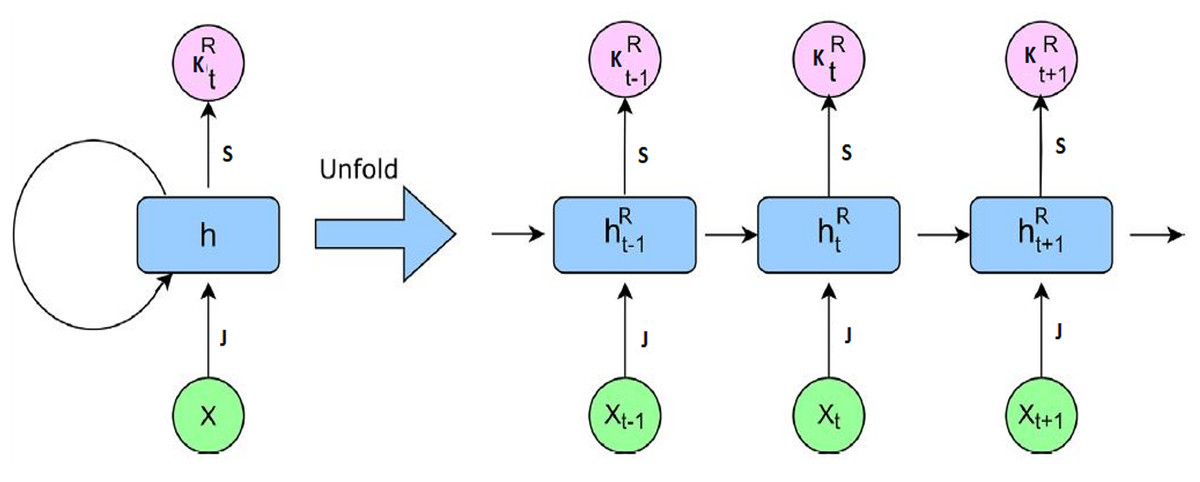
Figure 4: RNN model architecture.
Figure 4 illustrates the unfolded RNN architecture, where the hidden state is propagated forward through recurrent connections, enabling the model to learn how past atmospheric conditions influence future wind speed, thereby maintaining temporal continuity throughout the sequence. According to Fig. 4, the recurrent hidden state is computed as follows:
(1)
Here, S is the weight matrix for the current input, and J is the recurrent weight matrix for the previous hidden state . The bias term is denoted by b. The function v ( ) is a nonlinear activation such as ReLU. The hidden state is then transformed into an intermediate output vector as:
(2) where and are the output weights and bias, respectively. The feedback loop formed by allows temporal information to be retained and updated over time. During training, the network optimizes these parameters to minimize the prediction error. For prediction, is passed to a fully connected (FC) layer to produce the scalar output where is the FC layer weight matrix, and is its bias. Both are trainable parameters and optimized during training. For meteorological sequences, RNNs effectively capture short-horizon wind fluctuations such as diurnal or gust events.
The long short-term memory
The LSTM architecture was proposed by Hochreiter & Schmidhuber (1997) as a solution to the vanishing gradient problem. LSTMs extend the standard RNN architecture by introducing a memory cell and a gating mechanism that regulates the flow of information, enabling the network to capture effectively long-term dependencies on sequential data. Unlike RNN, LSTM has an input gate, a forget gate, and an output gate, as seen in Fig. 5.
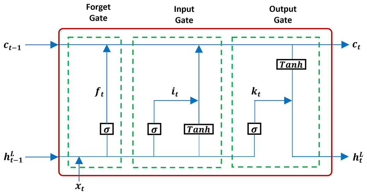
Figure 5: A structure of LSTM.
Based on Fig. 5, the formulation of equations in the LSTM framework is derived as follows:
(3)
(4)
(5)
(6)
(7)
(8)
Here:
is the input gate.
is the forget gate.
is the output gate.
-
( ) is the activation function.
is the input vector at time t.
is the hidden state from the previous time step.
S ( ) and J ( ) are the input and recurrent weight matrices for each gate.
b ( ) are bias terms for each gate.
is the candidate memory content, generated as a non-linear transformation of the current input and previous hidden state.
tanh ( ) is the hyperbolic tangent activation.
denotes elementwise (Hadamard) multiplication.
The roles of the gates are as follows:
Input gate (Eq. (3)) regulates how much new information enters the cell state, .
Forget gate (Eq. (4)) determines how much of the previous cell state is retained.
Output gate (Eq. (5)) controls how much of the updated cell state contributes to the hidden state output .
The cell state update in Eq. (7) blends newly candidate memory information of Eq. (6) with the retained memory . The hidden state is then mapped to the final output via the FC layer where and are the trainable weight and bias of the FC layer and optimized during training. For regression, a linear activation is applied to ensure can take any continuous value. The gating mechanism allows LSTMs to effectively preserve relevant information over extended sequences, making them highly suitable for wind speed prediction tasks where both short-term fluctuations and long-term seasonal trends are important.
The bidirectional LSTM
The BiLSTM network extends the standard LSTM by processing sequence data in both forward and backward directions. It employs two independent LSTM layers: one that captures dependencies from past to future (forward layer) and another that captures dependencies from future to past (backward layer). This dual processing enables the model to leverage both preceding and succeeding contexts, providing a more comprehensive representation of the sequence compared to unidirectional LSTMs. The BiLSTM architecture is illustrated in Fig. 6.
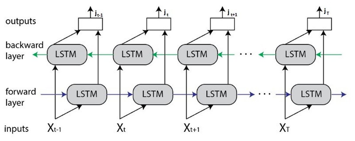
Figure 6: BiLSTM architecture.
As illustrated in Fig. 6, at each time step t, the forward LSTM generates a hidden state while the backward LSTM produces expressed as:
(9)
(10)
Here:
is the input vector at time t.
and are the previous and next hidden states in the forward and backward layers, respectively.
and are the corresponding cell states in the forward and backward layers, respectively.
and denote the LSTM functions applied in the forward and backward directions, respectively.
The outputs from the forward and backward hidden states are concatenated to form the BiLSTM feature vector at time step t:
(11)
Finally, for prediction, is passed through an FC layer to map the feature vector into the scalar target output where and are the trainable weight matrix and bias term of the output layer, respectively. Both parameters are optimized during training. BiLSTM networks offer significant advantages over unidirectional LSTMs, particularly in tasks where the entire sequence is available during training. By incorporating future context alongside past information, BiLSTMs can effectively manage long-range dependencies and capture more intricate temporal relationships. This makes them well-suited for wind speed prediction in the SCS, where both historical trends and upcoming atmospheric changes can influence short-term forecasts.
The proposed hybrid RNN and BiLSTM
We propose a two-stage recurrent architecture that combines the RNN layer as a feature extractor with a subsequent BiLSTM for context aggregation. At each time step t, the RNN transforms the raw input (the meteorological parameters: longitude, latitude, SST, t2m, msl, mtpr, and the 10m u and v wind components) into a compact representation (cf. Eq. (2)), emphasizing short-range temporal cues. The BiLSTM then consumes in both forward and backward directions to capture long-range dependencies from past and future context, after which the two directional states are concatenated and passed to an FC layer. The FC layer maps the high-dimensional concatenated features into the final wind speed prediction, .
The RNN layer is placed before the BiLSTM to extract short-horizon temporal patterns and suppress high-frequency noise before long-range aggregation. This order preserves and enhances the BiLSTM’s ability to learn bidirectional dependencies without losing context to the RNN’s shorter memory. Reversing the order would risk degrading long-term meteorological patterns, increase computational cost, and reduce interpretability for multi-scale wind variability in the SCS. The architecture of the proposed h-RNN-BiLSTM model, which includes the FC layer, is depicted in Fig. 7.
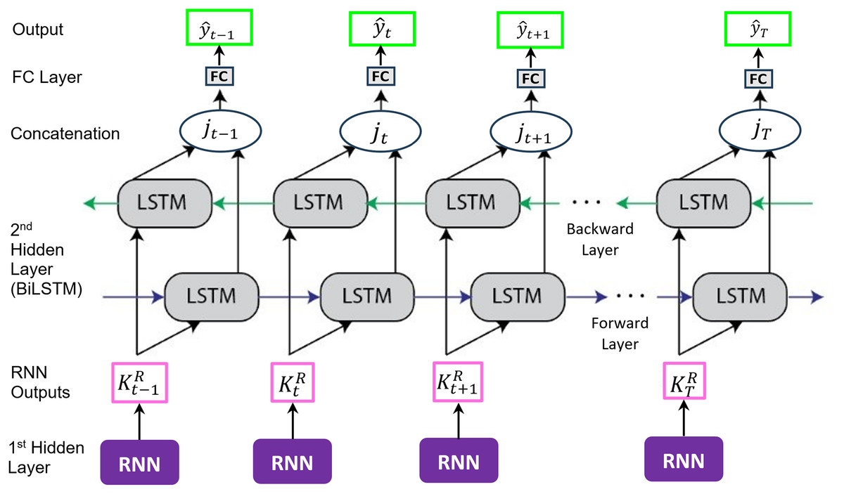
Figure 7: A hybrid RNN and BiLSTM (h-RNN-BiLSTM) architecture.
Based on the schematic in Fig. 7, the forward direction of the proposed h-RNN-BiLSTM framework can be formulated as follows:
(12)
(13)
(14)
(15)
(16)
(17)
The backward direction can be formulated as follows:
(18)
(19)
(20)
(21)
(22)
(23)
Here:
and are the input gates in the forward and backward directions, respectively.
and denote the forget gates in the forward and backward directions, respectively.
and represents the output gates corresponding to the forward and backward directions, respectively.
and are the previous and next hidden states in the forward and backward directions, respectively.
-
( ) is the activation function.
is the output from RNN model.
and are the current or updated cell states in the forward and backward directions, respectively.
and are the corresponding previous and next cell states in the forward and backward directions, respectively.
S ( ) and J ( ) are the input and recurrent weight matrices for each gate.
b ( ) are bias terms for each gate.
and are the candidate memory contents in the forward and backward directions, respectively.
tanh ( ) is the hyperbolic tangent activation.
denotes elementwise (Hadamard) multiplication.
In compact form, the proposed h-RNN-BiLSTM model is defined as follows:
(24)
(25)
Here, and denote the forward and backward hidden states, respectively. The two directional states are concatenated such that
(26) and mapped to the output
(27) where and are the weight matrix and the bias vector of the final FC output layer respectively. Both and are trainable parameters and optimized during training to minimize the prediction loss. No manual assignment of these values is required. The integration of short-term dynamics captured by the RNN with the long-term bidirectional dependencies modeled by the BiLSTM enables the proposed approach to effectively exploit the multi-scale wind variability characteristic of the SCS meteorological system. In this architecture, the RNN front-end emphasizes short-horizon dynamics (e.g., gustiness), while the BiLSTM aggregates bidirectional context to model the multi-scale temporal structure driven by monsoon transitions and synoptic variability in the region. This division of labor facilitates fine-grained pattern recognition and enhances generalization performance compared to using either the RNN, LSTM or BiLSTM in isolation.
Training the proposed h-RNN-BiLSTM model
The training process was conducted on both short-term and long-term datasets. The short-term datasets consisted of GFS and ECMWF records from 2 December 2022 to 31 May 2023, while the long-term dataset comprised ECMWF records from 1 January 2019 to 31 August 2023. Both datasets were prepared with temporal resolutions of 3 h. For each dataset, the training procedure involved feeding the standardized meteorological predictors (longitude, latitude, SST, t2m, msl, mtpr, and u/v wind components) into the h-RNN-BiLSTM architecture. The RNN layer first transformed the input sequence into compact feature representations, as described in Eqs. (1) and (2), emphasizing short-term temporal variations. These features were then processed by the BiLSTM layer in both forward and backward directions (Eqs. (12)–(23)) to capture bidirectional long-term dependencies. The concatenated output from the BiLSTM (Eq. (26)) was passed to the fully connected layer (Eq. (27)) to produce the final prediction
The proposed h-RNN-BiLSTM architecture was trained using 80% of the available data for model training and 20% for testing, for both the GFS and ECMWF datasets. All experiments were executed on a workstation equipped with an Intel Core™ i9-13900 processor, 64 GB of RAM, and an NVIDIA GeForce RTX 4090 GPU, running TensorFlow v2.9.1 (Python 3.8.8) within the Anaconda 4.3 environment. This computing setup ensured the capability to process large-scale meteorological time series efficiently and enabled rapid convergence during the training process. All hyperparameters were determined through a preliminary study conducted prior to the main experiments. This study systematically explored various model configurations to achieve an optimal trade-off between forecasting accuracy and computational efficiency. Specifically, different neuron counts were evaluated for the proposed h-RNN-BiLSTM architecture. Multiple activation functions, including tanh, sigmoid, and ReLU, were tested. Batch sizes of 32, 64, and 128 were examined and epoch counts ranging from 5 to 30 were considered. Finally, different optimizers, including stochastic gradient descent (SGD), RMSProp, and Adam, were compared.
The final model configuration consisted of h-RNN-BiLSTM layer with 50 neurons which represents the size vector (Eq. (24)) and (Eq. (25)) using the ReLU activation function, σ ( ) for its faster convergence and lower susceptibility to vanishing gradient issues. A fully connected output layer with one neuron was employed to produce scalar wind speed predictions (Eq. (27)). The Adam optimizer was chosen for its adaptive learning rate capability, which proved particularly effective for sequential meteorological data. Adam updates all trainable parameters in the h-RNN-BiLSTM and fully connected layers by computing the gradient of the MSE loss defined as:
(28) where is the actual wind speed, is the predicted value, and N is the total number of observations. Instead of computing Eq. (28) over the entire dataset at once, the MSE is computed over a mini batch of size = 64. This approach provides stable gradient updates while avoiding excessive memory consumption. In practice, the MSE loss is computed over 64 samples at a time, after which the Adam optimizer updates the model weights. Training was performed for 10 epochs, where an epoch corresponds to one complete pass through the training dataset. The choice of 10 epochs was determined to be sufficient for model convergence while reducing the risk of overfitting.
Testing and performance evaluation
Following model training, the optimized parameters (weights, and biases, ) in Eq. (27) were applied to the testing phase, which involved predicting wind speeds ( ) for unseen data. To evaluate the forecasting performance of the proposed model, this study employed two widely used error-based accuracy metrics: root mean squared error (RMSE) in Eq. (29) and mean absolute percentage error (MAPE) in Eq. (30). The RMSE metric provides an insight into the residual variance between the actual value and the predicted value , while the MAPE metric signifies the average absolute percentage deviation. Lower MAPE and RMSE values are preferred, indicating enhanced predictive accuracy.
(29)
(30)
The proposed h-RNN-BiLSTM model was benchmarked against established models including RNN, LSTM, BiLSTM, and the well-known statistical method, ARIMA, to demonstrate the effectiveness of the hybrid architecture.
Results
We conducted training, testing, and evaluation of the proposed hybrid model within the source domain under two experimental setups. Experiment 1 employed short-term datasets from both the GFS and the ECMWF, while Experiment 2 utilized long-term datasets from ECMWF.
Experiment-1: short-term GFS and ECMWF datasets
In the first experiment, the proposed h-RNN-BiLSTM architecture was trained using 80% of the short-term datasets from both the GFS and the ECMWF, covering the period from 2 December 2022 to 31 May 2023. The convergence behavior of the model was monitored using the mean squared error (MSE) of Eq. (28) during training. Figure 8 presents the MSE curves over 10 training epochs for both datasets.
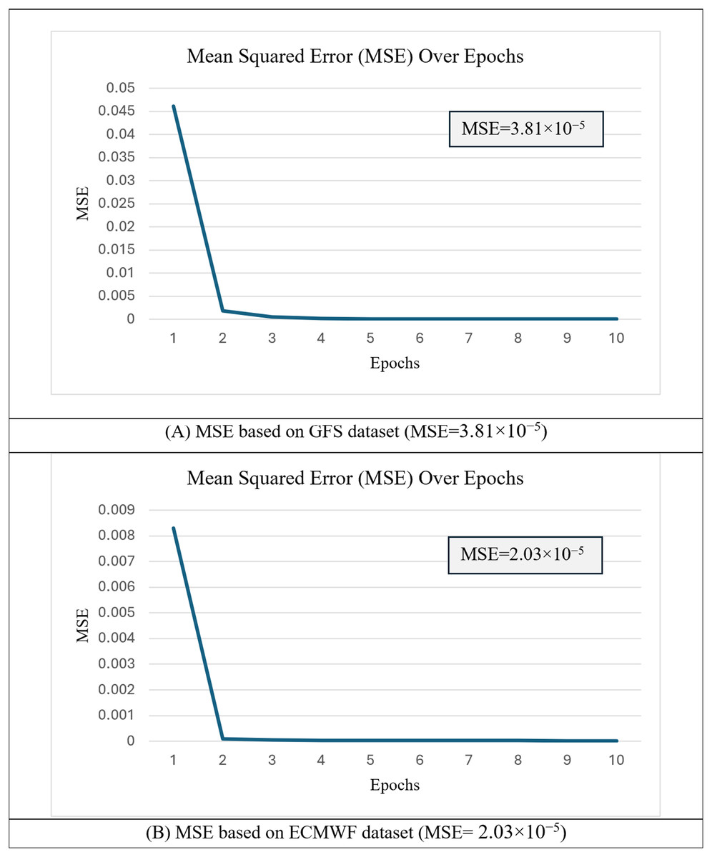
Figure 8: Mean squared error (MSE) over epochs during training of the h-RNN-BiLSTM model.
(A) MSE based on the GFS dataset (MSE = 3.81 × 10⁻⁵). (B) MSE based on the ECMWF dataset (MSE = 2.03 × 10⁻⁵).
As shown, the MSE values decreased steadily as the number of epochs increased, indicating stable convergence. The final MSE value for GFS was 3.81 × 10⁻⁵, while the corresponding value for ECMWF was 2.03 × 10⁻⁵. The consistently lower MSE for ECMWF suggests that this dataset provides more reliable and consistent atmospheric representations, which facilitates better generalization to unseen data. In all cases, the curves exhibited smooth convergence without significant divergence, demonstrating stable learning behavior with minimal signs of overfitting. These results confirm that the hyperparameters selected during the preliminary study (‘Training the Proposed h-RNN-BiLSTM Model’) were effective in achieving low errors while maintaining generalization capability across datasets. The optimized weights, and biases, from this training which correspond to Eq. (27) were then applied to the target domain model for wind speed ( ) prediction. The predicted wind speeds, generated by the proposed h-RNN-BiLSTM model were compared against actual wind speeds, using both scatter plots and time-series plots, as presented in Figs. 9 and 10.
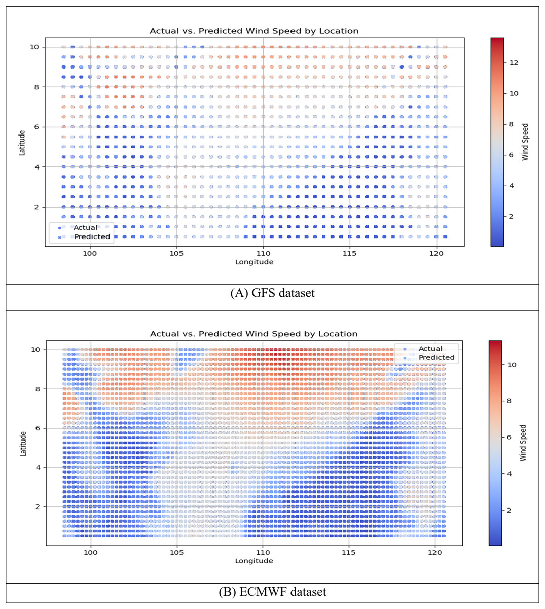
Figure 9: Scatter plots of actual vs. predicted wind speed for the h-RNN-BiLSTM model using (A) the GFS dataset and (B) the ECMWF dataset.
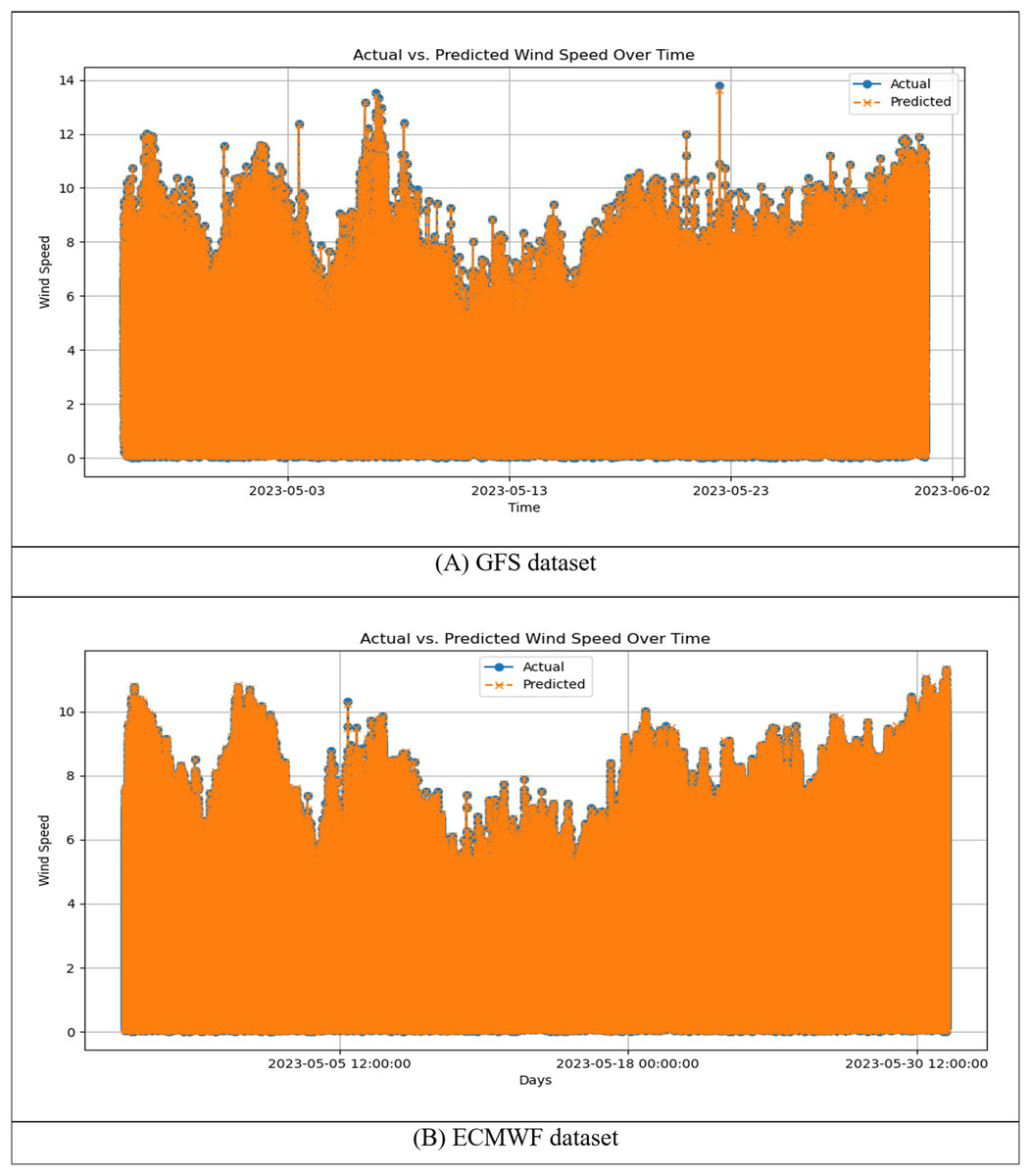
Figure 10: Time series plots of actual vs. predicted wind speed for the h-RNN-BiLSTM model using (A) the GFS dataset and (B) the ECMWF dataset.
Figures 9 and 10 illustrate the comparative performance of the h-RNN-BiLSTM model using the GFS and ECMWF datasets. Across both scatter plots (Fig. 9) and time-series plots (Fig. 10), the ECMWF-based configuration consistently outperformed the GFS counterpart. This closer alignment in the ECMWF dataset was evident in the tight clustering within the scatter plots and the minimal deviation observed in the time-series curves. These results indicate that ECMWF’s greater spatial resolution and temporal consistency provided a stronger foundation for short-term wind speed forecasting in the SCS. In contrast, while the GFS-based models captured the general patterns, they exhibited noticeably larger deviations, particularly at higher wind speeds. These visual findings are reinforced by the quantitative results in Table 1, which report the RMSE and MAPE values for ARIMA, RNN, LSTM, BiLSTM, and the proposed h-RNN-BiLSTM model.
| Model | GFS | ECMWF | ||
|---|---|---|---|---|
| RMSE | MAPE | RMSE | MAPE | |
| ARIMA | 2.2596 | 1.5345 | 4.0072 | 3.2114 |
| RNN | 0.0546 | 3.4781 | 0.0285 | 0.9153 |
| LSTM | 0.0935 | 5.0199 | 0.0306 | 1.6112 |
| BiLSTM | 0.0581 | 4.6780 | 0.0220 | 1.2859 |
| h-RNN-BiLSTM | 0.0148 | 0.9771 | 0.0104 | 0.5343 |
As shown in Table 1, the proposed h-RNN-BiLSTM consistently yielded the lowest RMSE values across all configurations, reflecting improved predictive accuracy in terms of RMSE and MAPE. Specifically, the model attained RMSE values of 0.0148 (GFS) and 0.0104 (ECMWF), representing substantial improvements over other deep learning baselines (RNN, LSTM, BiLSTM) and ARIMA. In terms of MAPE, which measures relative percentage error, the h-RNN-BiLSTM also delivered the best performance in most cases, particularly with ECMWF (0.5343) and GFS (0.9771). On the GFS dataset, the proposed model achieved substantial error reductions, lowering RMSE by 99.3% compared to ARIMA, 72.9% to RNN, 84.2% to LSTM, and 74.5% to BiLSTM. Comparable improvements were observed in MAPE, with accuracy gains of 36.3%, 71.9%, 80.5%, and 79.1% over ARIMA, RNN, LSTM, and BiLSTM, respectively. Consistent performance was also obtained on the ECMWF short-term dataset, where RMSE decreased by 99.7%, 63.5%, 66.0%, and 52.7% relative to ARIMA, RNN, LSTM, and BiLSTM, while MAPE was reduced by 83.4%, 41.6%, 66.8%, and 58.5% against the same baselines. These results highlight that the proposed hybrid model is particularly effective for high-frequency short-term forecasting, where minimizing both absolute and relative errors is critical. Conversely, ARIMA, while less accurate in terms of RMSE, remains competitive for coarser time intervals when MAPE is prioritized.
Experiment-2: long-term ECMWF datasets
In the second experiment, the proposed h-RNN-BiLSTM model was evaluated using long-term ECMWF datasets to assess its performance under extended temporal coverage. The training set comprised 80% of the data, spanning from 1 January 2019 to 31 August 2023. As in Experiment 1, Eq. (28) (the MSE) was adopted as the loss function, and the results are illustrated in Fig. 11.
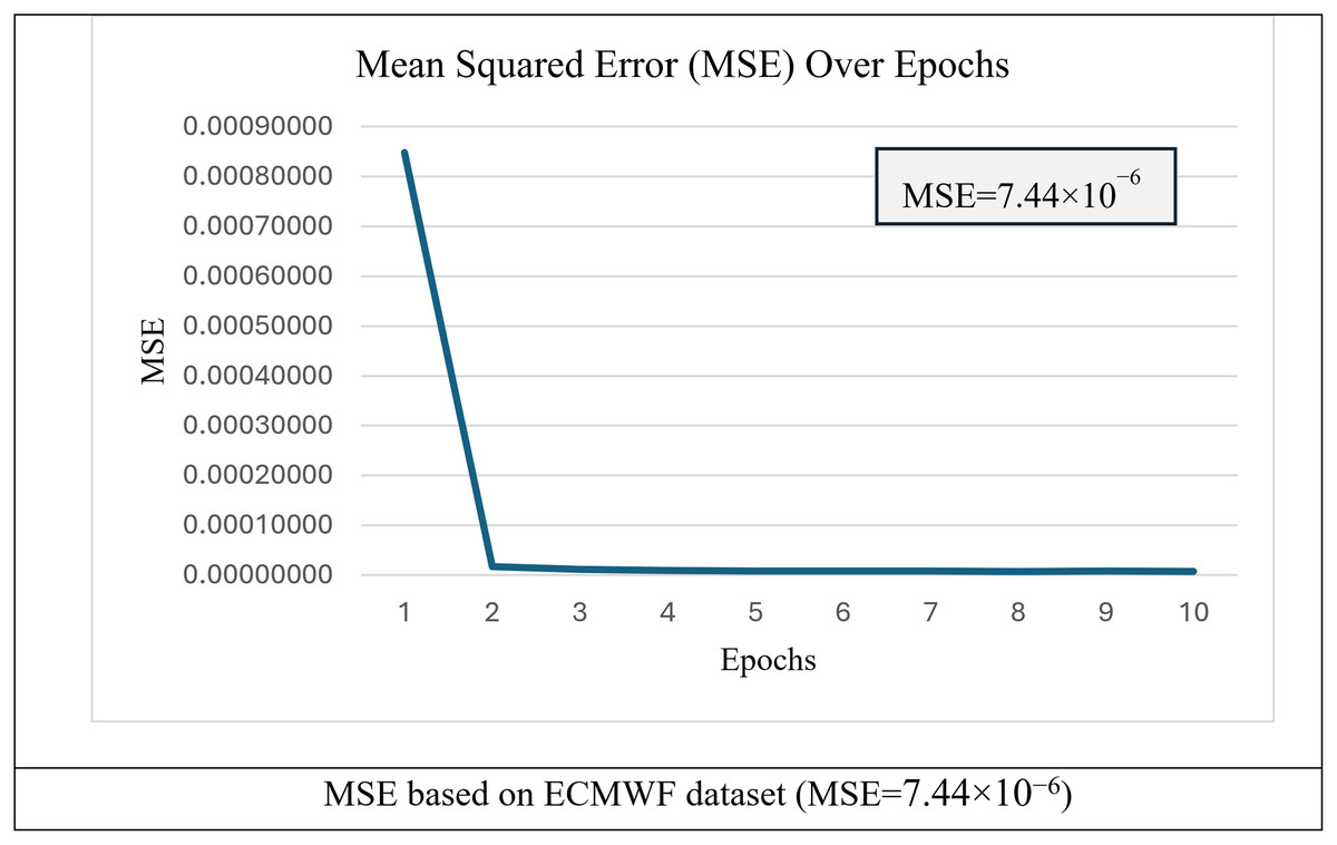
Figure 11: MSE over epochs for training of h-RNN-BiLSTM model.
Figure 11 shows the convergence behavior of the h-RNN-BiLSTM model when trained on the long-term ECMWF dataset. The loss decreased sharply within the first epoch and then stabilized, indicating efficient parameter optimization and convergence. The final MSE was 7.44 × 10⁻⁶, suggesting that the extended dataset supports more precise wind speed prediction. The training curve indicates stable learning without divergence, reducing the likelihood of overfitting across the long-time span. The optimized weights, and biases, from this training which correspond to Eq. (27) were then applied to the testing set to generate wind speed predictions, . Figure 12 presents scatter plots and time-series plots comparing actual and predicted wind speeds obtained using the proposed h-RNN-BiLSTM model.
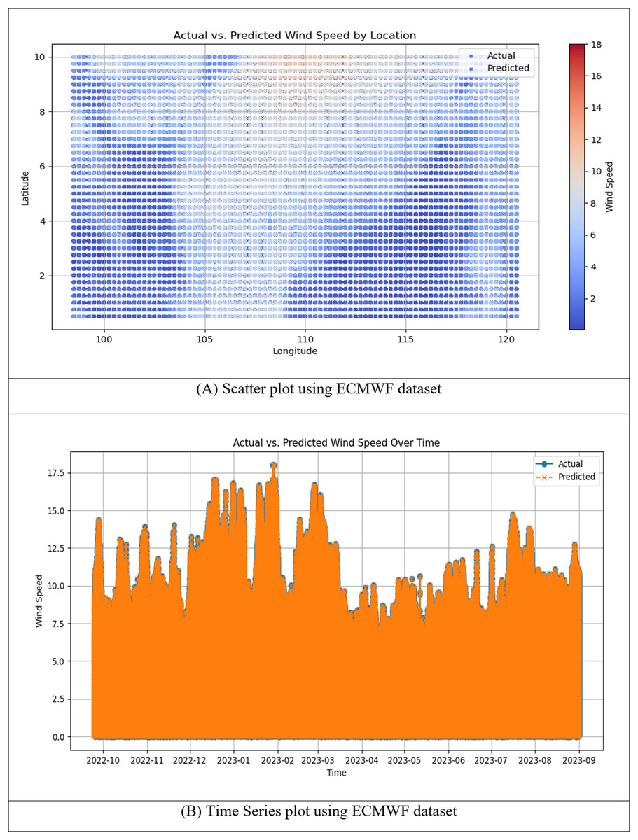
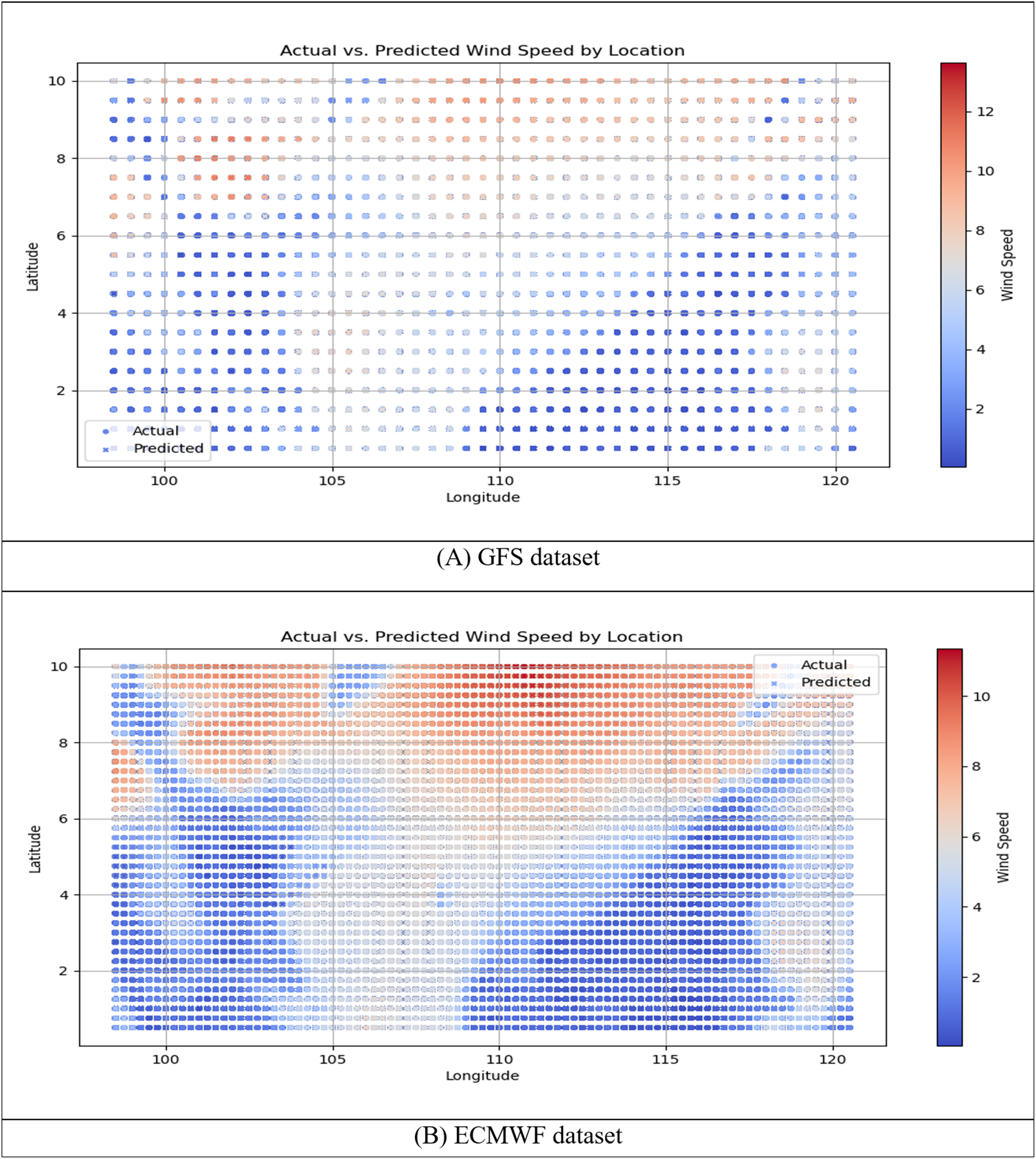
Figure 12: (A) Scatter plot and (B) time series plot of actual vs. predicted wind speed for the h-RNN-BiLSTM model using the ECMWF dataset.
Figure 12 illustrates the performance of the proposed h-RNN-BiLSTM model for wind speed prediction using long-term ECMWF datasets. The scatter plot in Fig. 12A shows the spatial distribution of actual and predicted wind speeds across the study domain. The predicted values closely follow the observed measurements, with only minor deviations across different latitudes and longitudes. This reflects a relatively consistent spatial agreement between actual and predicted values, indicating reliable spatial fidelity. The time series plot in Fig. 12B further demonstrates the model’s predictive accuracy across the full temporal span from 1 January 2019 to 31 August 2023. The predicted curves closely overlap with the actual wind speed measurements, effectively capturing both high-magnitude peaks and low-magnitude troughs with minimal phase shifts. The strong alignment with observed values, particularly during rapid wind speed fluctuations, suggests that finer temporal resolution improves the model’s ability to capture dynamic changes. Table 2 presents the RMSE and MAPE values for ARIMA, RNN, LSTM, BiLSTM, and the proposed h-RNN-BiLSTM models using long term ECMWF datasets.
| Model | RMSE | MAPE |
|---|---|---|
| ARIMA | 3.9736 | 2.9693 |
| RNN | 0.0357 | 0.7631 |
| LSTM | 0.0153 | 0.7827 |
| BiLSTM | 0.0170 | 0.6878 |
| h-RNN-BiLSTM | 0.0106 | 0.4671 |
Table 2 summarizes the RMSE and MAPE for ARIMA, RNN, LSTM, BiLSTM, and the proposed h-RNN-BiLSTM model using long-term ECMWF datasets. The h-RNN-BiLSTM achieved the lowest RMSE (0.0106) and MAPE (0.4671), consistently outperforming all baseline models. In terms of RMSE, the proposed model reduced error by 99.7% compared with ARIMA, 70.3% compared with RNN, 30.7% compared with LSTM, and 37.6% compared with BiLSTM. For MAPE, the improvements were 84.3% over ARIMA, 38.8% over RNN, 40.3% over LSTM, and 32.1% over BiLSTM. These percentage gains highlight the hybrid model’s effectiveness and its ability to capture both sequential dependencies (via RNN) and bidirectional temporal contexts (via BiLSTM). Overall, the findings confirm that h-RNN-BiLSTM consistently yields more reliable and accurate predictions across long-term datasets, making it well-suited for operational wind speed forecasting.
Discussion
This section synthesizes the findings from both Experiment 1 (short-term GFS and ECMWF datasets) and Experiment 2 (long-term ECMWF datasets) to interpret the performance of the proposed h-RNN-BiLSTM model in the context of wind speed forecasting for the SCS. The novelty of the h-RNN-BiLSTM lies in its architectural integration of two complementary recurrent units: the RNN front-end, which captures immediate short-term dependencies and efficiently models rapid fluctuations in wind speed such as gustiness, and the BiLSTM back-end, which models bidirectional long-term dependencies by utilizing both past and future contextual information within the input sequence. This division of labor between sequential components allows the model to extract multi-scale temporal features in a manner that has not been commonly explored in meteorological forecasting literature, where models are often limited to single RNN, LSTM and BiLSTM architectures or hybrids involving convolutional layers. By combining RNN and BiLSTM layers, the proposed approach leverages the strengths of both structures to deliver improved accuracy in capturing the complex temporal dynamics of wind speed.
The performance of the proposed h-RNN-BiLSTM model and baseline methods were assessed using two error-based metrics: RMSE and MAPE. RMSE, defined in Eq. (29), penalizes large deviations more heavily, making it particularly important for wind speed forecasting where extreme events such as gusts or squalls can have disproportionate operational impacts. MAPE, defined in Eq. (30), provides a normalized measure of forecasting accuracy that facilitates comparisons across datasets with different wind speed ranges. Taken together, these metrics offer a complementary view: RMSE captures robustness against large errors, while MAPE emphasizes relative precision across varying temporal resolutions and datasets. The inclusion of both metrics ensures that the evaluation is not biased toward either absolute or relative error, and it aligns with best practices in meteorological time-series forecasting literature.
According to the short-term dataset results presented in Table 1 from Experiment 1, the h-RNN-BiLSTM model achieved RMSE values of 0.0148 (GFS) and 0.0104 (ECMWF), which represent substantial improvements over the baseline models. Specifically, the proposed model reduced RMSE by 99.3% (vs. ARIMA), 72.9% (vs. RNN), 84.2% (vs. LSTM), and 74.5% (vs. BiLSTM) on the GFS dataset. Similar trends were observed in MAPE, where h-RNN-BiLSTM improved accuracy by 36.3% (vs. ARIMA), 71.9% (vs. RNN), 80.5% (vs. LSTM), and 79.1% (vs. BiLSTM). On the ECMWF short-term dataset, improvements remained consistent, with RMSE reductions of 99.7% (vs. ARIMA), 63.5% (vs. RNN), 66.0% (vs. LSTM), and 52.7% (vs. BiLSTM). The corresponding MAPE reductions were 83.4% (vs. ARIMA), 41.6% (vs. RNN), 66.8% (vs. LSTM), and 58.5% (vs. BiLSTM). These results demonstrate that the hybrid model effectively captures both sequential dependencies and bidirectional temporal dynamics, providing strong short-term predictive accuracy.
Table 2 presents the results of Experiment 2 using long-term ECMWF datasets. With the extended temporal coverage of 2019–2023, the h-RNN-BiLSTM model consistently achieved the lowest RMSE (0.0106) and MAPE (0.4671). Compared with ARIMA, the improvements were 99.7% (RMSE) and 84.3% (MAPE), highlighting the inadequacy of statistical models in handling nonlinear and long-range wind speed dynamics. Against deep learning baselines, the proposed model also delivered consistent gains: RMSE reductions of 70.3% (vs. RNN), 30.7% (vs. LSTM), and 37.6% (vs. BiLSTM), along with MAPE reductions of 38.8% (vs. RNN), 71.0% (vs. LSTM), and 32.1% (vs. BiLSTM). These findings confirm the hybrid model’s ability to sustain stable learning across extended periods, mitigating overfitting while ensuring precise long-term forecasts. In addition, the hybrid deep learning architecture benefits more from larger datasets and longer historical sequences, allowing it to learn richer temporal patterns that conventional statistical methods cannot capture. Individual models like RNN, LSTM or BiLSTM yielded less precise results, as Tables 1 and 2 demonstrate. Possible factors that can affect the outcome include individual models’ limited ability to accurately represent complex patterns and relationships in the dataset, a lack of coordination between short-term and long-term memory aspects, and a failure to effectively utilize the advantages of combined architecture for accurate prediction (Almeida, Neves & Horta, 2018; Yuan et al., 2023).
Another key observation is the effect of dataset length on the performance of the proposed model. When comparing short-term ECMWF (Table 1) with long-term ECMWF (Table 2), the RMSE values remain nearly identical (0.0104 vs. 0.0106), indicating consistent control of absolute errors across different temporal horizons. However, MAPE improved from 0.5343 in the short-term dataset to 0.4671 in the long-term dataset, reflecting a 12.6% improvement in relative accuracy. This suggests that the proposed h-RNN-BiLSTM is particularly suitable in maintaining proportional predictive accuracy when trained on longer datasets due to the richer temporal dependencies captured over extended periods. This stability across forecasting horizons demonstrates the adaptability of the model, an important attribute for practical deployment in meteorological forecasting where both short-term and long-term accuracy are essential. The comparative analysis also highlights the utility of combining short-term and long-term evaluations for validating model accuracy. In operational contexts, short-term datasets are often used for immediate forecasting, whereas long-term datasets are critical for climate-informed planning and energy management. The ability of h-RNN-BiLSTM to achieve stable RMSE and improved MAPE across both settings confirms its potential applicability in diverse scenarios, ranging from wind forecasting to strategic planning for renewable energy integration. Thus, the model offers technical advantages over existing approaches and is practically relevant for meteorological and energy-related applications.
However, certain limitations should be acknowledged. The model’s performance is sensitive to data quality and completeness where gaps or inconsistencies in historical records can reduce forecasting reliability. While the primary focus of this study is forecasting accuracy, we also emphasize that the proposed h-RNN-BiLSTM model incurs longer training and testing times compared to baseline models due to its deeper architecture. Specifically, training required 23.2 s and testing 5 s for the short-term GFS dataset, 107.6 and 27 s for the short-term ECMWF dataset, and 816.1 and 158 s for the long-term ECMWF dataset (2019–2023). Importantly, the testing phase remains computationally manageable, indicating that once trained, the h-RNN-BiLSTM model can generate forecasts rapidly, making it suitable for near real-time wind speed prediction. Although the higher training cost reflects the model’s recurrent and bidirectional layers, the relatively low inference time suggests that efficiency is not a bottleneck for operational forecasting scenarios.
Conclusion
This study introduced an h-RNN-BiLSTM model for wind speed forecasting in the South China Sea and evaluated its performance using short-term GFS/ECMWF datasets and long-term ECMWF datasets. The evaluation employed RMSE and MAPE as performance metrics, providing detailed insights into both error magnitudes and relative accuracy. The experimental results revealed that the h-RNN-BiLSTM model consistently achieved the lowest RMSE and MAPE across all datasets. Improvements ranged from 30% to over 99% in RMSE and 32% to over 84% in MAPE, depending on the baseline and dataset considered. These findings demonstrate the hybrid model’s advantage over statistical method and standalone deep learning architectures. More importantly, they highlight its ability to balance short-term accuracy with long-term stability, which is essential for real-world forecasting applications. The novelty of this work lies in its hybridization strategy, which effectively integrates RNN with BiLSTM. From a modeling perspective, the architecture effectively integrates the short-term temporal dynamics captured by the RNN layer with the long-term bidirectional dependencies modeled by the BiLSTM, enabling multi-scale representation of wind speed variability; a defining characteristic of meteorological systems in the SCS. This design yields improved generalization across different datasets. The comparative results against multiple baselines establish clear empirical evidence of the model’s contribution. From an application perspective, the proposed approach is particularly relevant to renewable energy integration, grid management, and long-term planning of wind power resources, where reliable forecasting is crucial for ensuring energy stability and efficiency.
These combined technical and practical implications indicate that the h-RNN-BiLSTM can function not only as a high-performing research prototype but also as a viable component in operational forecasting workflows. Although the hybrid model demonstrates clear performance gains over baseline methods, its accuracy remains contingent on the availability of high-quality, continuous historical data, as gaps or inconsistencies may undermine predictive reliability. Furthermore, enhanced capability comes at the cost of increased computational demands during training, which warrants careful consideration in real-world deployments. While training times were longer due to the model’s deeper recurrent and bidirectional layers, the prediction phase remained rapid, enabling near real-time wind speed forecasting. This balance of accuracy and efficiency underscores the model’s potential for practical application in meteorological forecasting and renewable energy integration. Future research directions include: (i) integrating additional meteorological variables (e.g., temperature, pressure, and humidity) as multivariate inputs, (ii) fusing multiple reanalysis and observational datasets to improve generalization across regions, (iii) incorporating advanced attention mechanisms to strengthen temporal dependency modeling, (iv) extending the framework to other geographic contexts to evaluate its transferability, and (v) investigating the efficiency aspect, including optimization of execution time and memory usage, to support real-time forecasting and practical deployment in offshore and marine applications.