
System recovery of MIMO nonlinear systems against false data injection attack
- Published
- Accepted
- Received
- Academic Editor
- Davide Chicco
- Subject Areas
- Algorithms and Analysis of Algorithms, Data Science
- Keywords
- System recovery, Cyber-physical system, Attack-compensation, False data injection attack, Nonlinear systems, Feedback-linearization
- Copyright
- © 2025 Liang et al.
- Licence
- This is an open access article distributed under the terms of the Creative Commons Attribution License, which permits unrestricted use, distribution, reproduction and adaptation in any medium and for any purpose provided that it is properly attributed. For attribution, the original author(s), title, publication source (PeerJ Computer Science) and either DOI or URL of the article must be cited.
- Cite this article
- 2025. System recovery of MIMO nonlinear systems against false data injection attack. PeerJ Computer Science 11:e3280 https://doi.org/10.7717/peerj-cs.3280
Abstract
This article investigates the system recovery problem for a class of multi-input multi-output (MIMO) nonlinear systems under false data injection attack. Under the conditions that the attack is norm-bounded and the system has a vector relative degree and a trivial zero dynamics, the nonlinear system is transformed into a linear one by means of feedback-linearizing design. Then, a high-gain approximate differentiator is adopted to obtain the system states with any arbitrary accuracy. After that, by using a technique of replacing real-time with a small time delay, a recursive attack-compensation input signal is constructed and added into the system input to almost fully compensate for the impact of the attack on the system’s transient performance. At this time, the input of the nonlinear system includes two parts: desired input (or called reference input), which is designed according to the nominal model, and additional attack-compensation input. Theoretical analysis shows for the first time that the system can be almost fully recovered in the sense of the mapping relationship between the desired input and nonlinear system states, i.e., the aforementioned mapping is almost the same as the one in the nominal system. Finally, a simulation on a near-space vehicle is provided for verifying the theoretical results.
Introduction
The integration of computation, communication and control units has led to the birth and rapid development of a new generation of intelligent systems (Khan et al., 2025b; Alsinai et al., 2025), i.e., the cyber-physical systems (CPSs), which have been increasingly used in transportation systems, smart grids, power systems, remote surveillance and other fields (Cheng, Shi & Sinopoli, 2017). Due to the openness of information exchange and the complexity of physical dynamics, the long-time running of CPSs may cause security problems (Alrslani et al., 2025). Security vulnerabilities of CPSs provide the malicious attackers with the opportunity to implement them with ulterior motives (Khan et al., 2025a).
Generally, the cyberattacks can be broadly categorized as three main categories: denial-of-service (DoS) attacks, replay attacks and false data injection (FDI) attacks. DoS attackers obstruct the communication between networked agents (Wang et al., 2025). Relay attackers record and cover the communication data to degrade the system performances (Markantonakis et al., 2024). Different from them, FDI attacks, which intend to tamper transmitted data packages causing false feedback information, are more dangerous and complicated (Li, Shi & Chen, 2018). For this reason, the researches on CPSs under FDI attacks recently become one of the main topics.
In the past decade, fruitful results have been made for CPSs under attacks on attack strategy design (Zhang & Ye, 2020b; Zhang, Ye & Shi, 2022), attack detection (Alfriehat et al., 2024; Tanyıldız et al., 2025), secure estimation (Sun & Yang, 2025) and secure control (Yang et al., 2024; Khan et al., 2025c). To name a few, based on self-generated FDI attacks, Zhang & Ye (2020b) proposed a necessary and sufficient condition for attack parameters such that FDI attacks can achieve complete stealthiness. Subsequently, they investigated decentralized FDI attacks that destabilize the estimation error dynamics but eliminate their influences on the residual in each sensor node. Pasqualetti, Dörfler & Bullo (2013) designed centralized and distributed attack detection and identification monitors for continuous-time descriptor systems. In addition, secure estimation and secure control have also received great attention, especially in recent years. In An & Yang (2019), with the help of a constrained set partitioning approach, a state estimation scheme was proposed for discrete-time linear CPSs to relieve the computational complexity on the premise of the estimation correctness. Besides, they also investigated the secure control problem for nonlinear interconnected systems against intermittent DoS attacks (An & Yang, 2018a). Although these approaches proved their efficiency in attack design, attack detection, secure estimation and secure control, they ignored the impact of the attack on the system itself and did not consider how to recover the system. Actually, depending on desired precision and safety criticality of a system, changes in the transient response can be highly undesirable (Chakrabortty & Arcak, 2007, 2009). This inspired research on performance recovery (Atassi & Khalil, 1999).
In the past dozen years, performance recovery for nonlinear control has begun to attract attention in the literature, where the controller recovers the nominal transient trajectory in the presence of plant uncertainties and external disturbances. Such results for certain nonlinear control designs were proved in Back & Shim (2007, 2009), Chakrabortty & Arcak (2007, 2009), where singular perturbation methods are adopted to prove performance recovery. However, disturbance and its derivative are assumed to be bounded in Back & Shim (2007, 2009), and the uncertainty is assumed to be a sufficiently smooth function in Chakrabortty & Arcak (2007, 2009). Additionally, the tracking problem was studied in Freidovich & Khalil (2008) for a partially feedback linearizable single-input-single-output (SISO) nonlinear system with stable zero dynamics, where the closed-loop system under the observer-based controller recovers the performance of the nominal linear model as the observer gain becomes sufficiently high. However, the disturbance and its derivative are required to be bounded. An extension of Freidovich & Khalil (2008) to multi-input multi-output (MIMO) nonlinear systems was presented in Wang, Isidori & Su (2015) where the system is required to have a well-defined vector relative degree. After that, in order to relax the condition on vector relative degree, Wu et al. (2019) investigated the performance recovery for MIMO nonlinear systems under the (substantially weak) assumption of invertibility. One should note that the uncertainty is required to be a smooth function in Wang, Isidori & Su (2015), Wu et al. (2019). Despite these efforts on performance recovery for nonlinear systems, a common drawback of them is that the disturbances or uncertainties are differentiable, even smooth. For the attack signal, it is deliberately designed by hackers to harm the system. Thus, the attack signal may be a discontinuous and fast changing signal. This feature makes the existing results on performance recovery cannot be applied to CPSs under FDI attacks without assumption on its derivative, and to our knowledge, there is still no result available on system recovery problem of CPSs under attacks. This motivates the present study.
To more intuitively demonstrate the necessity of researching the system recovery problem for MIMO nonlinear systems under attack, Table 1 compares the proposed approach with existing methods.
| Methods | Robustness | Strengths or weaknesses |
|---|---|---|
| Secure control, e.g., Back & Shim (2007, 2009) | Enhancing the robustness of the controller | / |
| Back & Shim (2007, 2009) | Performance recovery | Disturbance and its derivative are assumed to be bounded |
| Chakrabortty & Arcak (2007, 2009) | Performance recovery | Uncertainty is assumed to be a sufficiently smooth function |
| Freidovich & Khalil (2008) | Performance recovery | Disturbance and its derivative are required to be bounded |
| Wang, Isidori & Su (2015), Wu et al. (2019) | Performance recovery | Uncertainty is required to be a smooth function |
| Our approach | System recovery (enhancing the robustness of the plant) | Only boundedness of the attack is required |
This article deals with the system recovery problem for a class of MIMO nonlinear systems subject to FDI attacks without assumption on its derivative. The system under consideration has a vector relative degree and a trivial zero dynamics, which can be transformed into a linear one by means of feedback-linearizing design. Then, a recursive attack-compensation input signal is constructed skillfully and added into the system input to almost fully compensate the attack, so that the system can be almost fully recovered. Compared to the existing results, our approach consists of the following main contributions and advantages: (i) A new perspective is provided for designing attack compensation scheme by compensating for the state deviation caused by the attack, which is helpful for designing an attack-compensated signal to recover the system. In fact, unlike the existing methods that enhance the robustness of control algorithms (e.g., Yang et al., 2024), the proposed method enhances the robustness of the plant itself; (ii) The existing results on CPSs mainly focus on attack design, attack detection, state estimation and secure control, but do not consider the state deviation of the system caused by the attack. In contrast, this article systematically investigates the recovery of CPSs under attacks for the first time; (iii) A common limitation of performance recovery for nonlinear system is that disturbances or uncertainties are required to be differentiable, even smooth (Back & Shim, 2007, 2009; Chakrabortty & Arcak, 2007, 2009; Freidovich & Khalil, 2008; Wang, Isidori & Su, 2015; Wu et al., 2019). Unlike disturbances and uncertainties, the attacks under consideration are not restricted to be differentiable or smooth.
Notations: Let represent the infinitesimal of the same order as T. For a matrix A, let A′ denote its transpose and denote its minimum eigenvalue. is called the Lie Derivative of with respect to . For any positive integer , denotes a shift matrix of dimension, , and . For a matrix , the notation represents the pseudo-inverse.
Problem statement
Consider the system recovery problem of the following MIMO nonlinear systems under FDI attack,
(1) where , and denote the state vector, the control input and the output, respectively. , and are known smooth mappings with and . The vector denotes the norm bounded FDI attack (Zhang & Ye, 2020b; Zhang, Ye & Shi, 2022), which is injected into the system by a malicious attacker.
Remark 1. Although represents an attack in this article, it can also be used to represent actuator faults, process faults, additive uncertainties, unknown inputs, external disturbances, or a combination of them (Arab et al., 2025).
Definition 1. (Isidori, 1985) A multivariable nonlinear system of the form Eq. (1) has a vector relative degree at a point if the following two conditions hold:
(i) for all , , , and for all in a neighborhood of , the following Lie Derivative
(2)
holds where .
(ii) the matrix
(3)
is row full rank at .
Assumption 1. The system Eq. (1) has a vector relative degree for all , and has a trivial zero dynamics.
Under Assumption 1, with the help of the Structure Algorithm (Teel & Praly, 1995; Freidovich & Khalil, 2008), there exist a diffeomorphism
(4) which brings the system Eq. (1) to the system modeled by equations of the normal form:
(5) with , , where is the -th row of and .
Assumption 2. There exists a positive constant number such that
(6)
Remark 2. For Assumption 1, some practical systems are capable of meeting it, such as high-speed train system (Zhang et al., 2024; Xie et al., 2025) and near-space vehicle system (Yao, Tao & Jiang, 2016). In addition, Assumption 2 can be found in Back & Shim (2007), Freidovich & Khalil (2008), Wang, Isidori & Su (2015), and this assumption is necessary to ensure the boundness of the signal which is injected into the nominal system by the attacker.
By feedback linearization, the input of the system Eq. (5), which is also the input of the system Eq. (1), is designed against the attack as
(7) with , where denotes the desired input (or called reference input) which is designed according to the nominal model, and is the attack-compensation signal which is added into the system input and will be designed skillfully to almost fully compensate the attack .
Under the above system input Eq. (7), the input-output model Eq. (5) will be transformed into the following linear one
(8) where , , , , , and the operator builds a block diagonal matrix from its argument. Furthermore, one can check that is bounded under Assumption 2.
For convenience of expression, let , and denote the nominal values of , and respectively (i.e., the values in the attack-free system or called the values in the nominal system). That is, , and satisfy
(9) with and .
Design objective: The purpose of this article is to design the additional attack-compensation input in Eq. (7) for the MIMO nonlinear system Eq. (1) such that the mapping relationship between the desired input and system states is almost the same as the one in the nominal system. In other words, the attack is almost fully compensated such that the system under consideration is almost recovered.
For the linear system Eq. (8), since which violates the observer matching condition (Corless & Tu, 1998), the attack-related term is hard to be estimated and compensated effectively by the existing results. Fortunately, this system has another obvious feature which makes it possible to almost completely compensate for the attacks-related term . That is, all states of the linear system Eq. (8) are derivatives of the output, i.e., for all and . Many approaches (e.g., high-gain approximate differentiators (Kalsi et al., 2010) and sliding mode exact differentiator (Floquet, Edwards & Spurgeon, 2007)) have been proposed to obtain the estimation of system states. As in Kalsi et al. (2010), the following lemma is established to obtain the system states with any arbitrary accuracy.
Lemma 1. (Kalsi et al., 2010) Consider the linear system Eq. (8). For the following high-gain observer Eq. (10) under Assumptions 1–2 and the boundness of , there exist a positive constant and a finite time such that for where denotes the start time of the system Eq. (1). Moreover, .
(10)
with , where denotes the estimation of , and are selected such that the roots of have negative real part. is defined with .
Obviously, one can see easily from Lemma 1 that can be replaced by with any arbitrary accuracy. For this reason and the convenience of description, it is reasonable to assume that is available for system recovery design. Also, the system input Eq. (7) can be rewritten as
(11) where represents the inverse operator of .
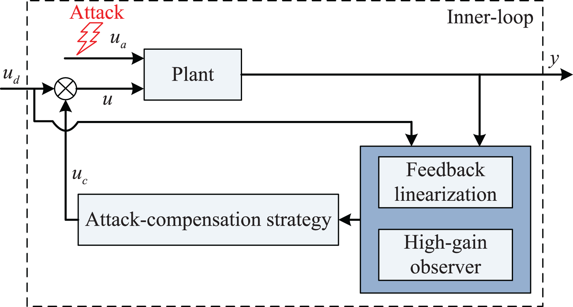
In order to show the proposed system recovery strategy more clearly, its block diagram is drawn in Fig. 1. The proposed attack-compensation strategy has the following obvious feature: it is an inner-loop controller so that it can be added on the existing closed-loop system working in harmony with a pre-designed outer-loop controller.
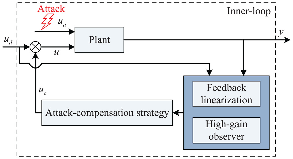
Figure 1: Block diagram of the proposed system recovery strategy.
System recovery design in a recursive fashion
Define an auxiliary variable with
(12) for all , where the parameters are selected such that the roots of the equation have negative real parts.
Obviously, can be rewritten as
(13) where with .
According to the knowledge of calculus, meets
(14) where denotes the start time of the system under consideration.
Before analyzing the impact of attacks on the original nonlinear system Eq. (1), we first analyze the impact of attacks on auxiliary variable which will provide great convenience for analyzing the original system. So let’s start now. If can fully compensate for the impact of the attack on the auxiliary variable , the following condition must be satisfied obviously.
(15) that is, . In other words, is required to be known in real-time a priori. Nevertheless, this condition is too strict for many practical systems, and thus, the following problem will naturally be encountered: whether the impact of the attack on the auxiliary variable can be compensated by removing the aforementioned restriction? The answer happens to be yes, and we will show that the impact of the attack on can almost completely compensated by a skillfully designed attack-compensation input signal .
The design process of the attack-compensation input signal includes the following two steps.
Step 1: Removing the strict requirements of real-time.
In order to eliminate the strict requirement of real-time, small time-delay will be adopted to replace real-time. In details, for the auxiliary variable in Eq. (14), we divide the whole time-domain of the right-hand side into interval segments with period , as follows
(16) where represents any positive integer and the positive constant T is called the period of compensation signal. Also, T is a small positive constant which denotes the small time-delay.
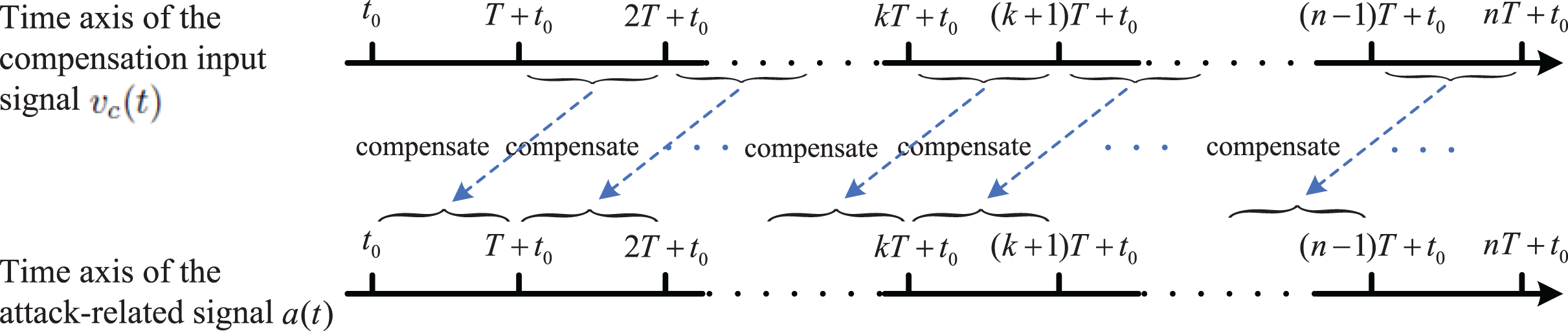
To remove the strict requirement of real-time, one way is to adopt in the interval for compensating the impact of on auxiliary variable in the interval (please see Fig. 2). Obviously, by choosing a small T, the attack can still be compensated timely to avoid the continuous impact of the attack on the auxiliary variable . According to this design thinking, , let
(17)
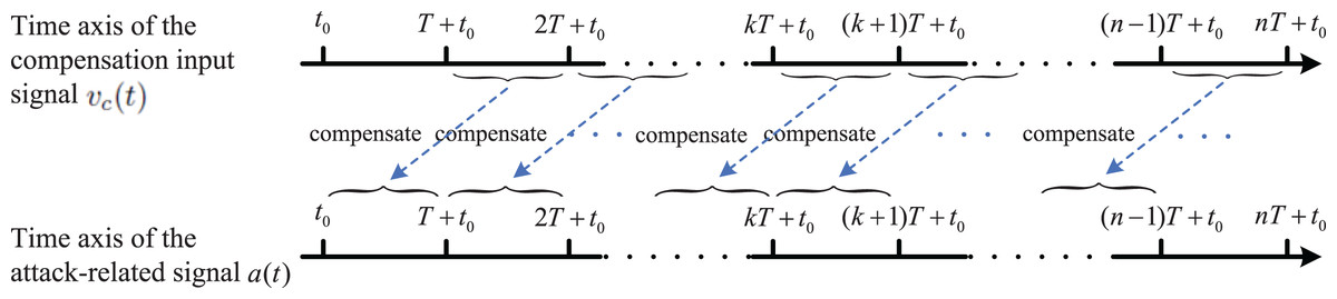
Figure 2: Block diagram of the attack-compensation strategy based on a small time-delay.
Under Eq. (17), one has
(18)
Obviously, when T is small enough, . One can see that, at time instants , the auxiliary variable is almost the same as the one in the nominal system (when the system is not attacked). Thus, at time instants , the attack-compensation input signal defined in Eq. (17) can almost eliminate the impact of on the auxiliary variable with a small time-delay T. It should be pointed out that the same result can be guaranteed for the interval which will be proved in the next section.
By some mathematical calculation, Eq. (17) can be rewritten for all as
(19) which is equivalent to
(20)
Let . By substituting it into Eq. (20), one has
(21) where we have used the fact that is invertible since the pair is controllable and L is row full rank. Therefore, it is pretty easy to obtain for all and that
(22) which is equivalent to
(23) holds for all and . Unfortunately, in Eq. (23) is not directly implementable if the attack signal is unknown. In the following Step 2, we will propose an alternative approach to solve the above problem.
Step 2: An alternative approach for solving the term .
It is easy to get from Eq. (8) that
(24)
With the help of Steps 1–2, and by combining Eqs. (23) and (24), one can obtain the following causal and implementable recursive attack-compensation input signal
(25) which holds for all and .
Remark 3. The term of is an infinitesimal of the same order as T. Thus, ill-conditioned matrix inversion will not be occurred in the calculation process of .
Remark 4. One can see from Eq. (23) that when , which implies that when . Therefore, the attack-compensation input signal will be disappeared and doesn’t change any system dynamics when the system is not attacked. This reflects one of the merits of the proposed method: it is easy to implement in practical systems.
Note that, the boundness of is required to be satisfied a priori of the high-gain observer Eq. (10) in Lemma 1. This condition is quite easy to satisfy, as will be proved in the following.
Theorem 1. Consider the linear system Eq. (8), and the attack-compensation input signal Eq. (25). Under the assumptions that the FDI attack signal is norm-bounded and stabilizes the following system Eq. (28), then and are both uniformly bounded.
Proof On the one hand, for , one can see from Eq. (23) that
(26) which implies that the signal is uniformly bounded. Also, one can further check that
(27)
On the other hand, let’s consider the linear system Eq. (8), which can be rewritten as
(28) where the pair is controllable, and is bounded since and are both bounded. Thus, according to Lyapunov stability theorem, it is pretty easy to see that is uniformly bounded when stabilizes the system Eq. (28).
Stability analysis
In this section, the stability of the original nonlinear system Eq. (1) with the system input Eq. (11) will be established.
Let denote the nominal value of the signal . That is,
(29) with .
Now, let us analyze the impact of the attacks on the auxiliary variable .
Theorem 2. Consider the linear system Eq. (8), and the attack-compensation input signal Eq. (25). Under Assumptions 1–2 and the assumption that stabilizes the system Eq. (28), then there exists an upper bound of which is an infinitesimal of the same order as T, where denotes the deviation caused by the attack. Also, can be arbitrary small when a small enough period T is selected.
Proof The proof is divided into the following two cases: (1) ; and (2) .
Case 1: . It is quite natural to obtain from Eqs. (8), (9), (14) and (29) that
(30) where .
Case 2: . One can see from Eqs. (14) and (29) that
(31)
Therefore, with the help of Eq. (23), the deviation satisfies
(32) where the first term on the right-hand side of the above inequality for obeys that
(33)
Combining Eqs. (32) and (33), one can conclude that
(34) holds for , where .
To sum up, one can conclude from Cases 1-2 that the deviation satisfies
(35) where we have used the fact that , and is bounded under Assumption 2. The right-hand side of the above inequality is an infinitesimal of the same order as T, and thus can be arbitrary small when a small enough period T is chosen. Hence, the proof is completed.
In the sequel, let us analyze the impact of attacks on the linear system Eq. (8).
Theorem 3. Consider the linear system Eq. (8), and the attack-compensation input signal Eq. (25). Under assumptions of Theorem 2, then there exists an upper bound of which is an infinitesimal of the same order as T, where denotes the state deviation caused by the attack and represents the nominal value of (i.e., the value in the attack-free system). Also, can be arbitrary small when a small enough T is selected.
Proof It is can be seen easily form Eqs. (9), (12) and (29) that
(36) holds for , where with .
Also, Eq. (36) can be rewritten as
(37) where is Hurwitz since are selected such that the roots of the equation have negative real parts. One can see from Eq. (37) that . Since is Hurwitz, it is always exists an invertible matrix such that , where denotes the diagonal matrix with the eigenvalue of on its main diagonal. Thus, one has
(38) where denotes the minimum eigenvalue of and we have used the fact that .
Furthermore, one can see from Eq. (36) that
(39)
To sum up, it is easy to get that is an infinitesimal of the same order as T, and thus can be arbitrary small when a small enough T is chosen.
Next, let us analyze the impact of attacks on the original nonlinear system Eq. (1).
Theorem 4. Consider the original nonlinear system Eq. (1), and the system input Eq. (11) with the attack-compensation input signal Eq. (25). Under assumptions of Theorem 2, then there exists an upper bound of which is an infinitesimal of the same order as T, where denotes the state deviation caused by the attack. Furthermore, the system is almost fully recovered when a small enough T is selected.
Proof One can see from Assumption 1 that there exists a diffeomorphism such that
(40) and thus
(41) where denotes the Lipschitz constant of the differentiable function in the compact set .
It is worth noting that, , together with Theorem 3, one has
(42)
Naturally, , which means that the system states under attacks can approximate the nominal states with arbitrary accuracy when a small enough T is selected.
In addition, let denote the nominal value of the desired input . That is, . Similarity, based on the facts that are smooth functions and , it is easy to prove that when T is small enough.
To sum up the above arguments, one can conclude that
(43)
Thus, the mapping relationship between the desired input and system states is almost the same as the one in the nominal system when T is small enough. In other words, the system is almost fully recovered when T is small enough.
Remark 5. Compared with the existing results on the secure control of CPSs (Deng & Wen, 2020; Xu et al., 2019; Feng & Hu, 2019; Zhang & Ye, 2020a; Yang et al., 2020; Wang et al., 2020; Yang, Li & Yue, 2020; Zhang, Shen & Han, 2019; Shao & Ye, 2020; An & Yang, 2018a; Su & Ye, 2018; Hu et al., 2019; Chen et al., 2021; Wu et al., 2021; Gu et al., 2021; Huang & Dong, 2020; He et al., 2021; Chen et al., 2022b; Farivar et al., 2019; Chen et al., 2022a; Lu & Yang, 2017; He et al., 2020; An & Yang, 2018b; Ao, Song & Wen, 2018; Zhou et al., 2020; Chen et al., 2022b), there are several merits of the proposed system recovery scheme: (i) the proposed method can be well applied to the existing methods, because the system can be almost fully recovered; (ii) the proposed approach not only can ensure a good enough performance, but also does not require any knowledge of attack’s model and other strict-preconditions; (iii) the proposed approach helps to ensure state performances and state constraints, since the proposed attack-compensation approach can ensure that the trajectory of the system states is almost not affected by the attack.
Remark 6. In existing results for nonlinear systems (Back & Shim, 2007, 2009; Chakrabortty & Arcak, 2007, 2009; Freidovich & Khalil, 2008; Wang, Isidori & Su, 2015; Wu et al., 2019), performance recovery was investigated for compensating the disturbances or uncertainties. A common limitation of these results is that the disturbances or uncertainties are required to be differentiable, even smooth. However, the proposed method is not subject to this limitation; and unlike the disturbances and uncertainties, the attacks under consideration are not restricted to be differentiable or smooth. Furthermore, this article systematically studies the system recovery of CPSs under attacks for the first time.
Remark 7. Generally speaking, the smaller the value of the positive parameter T, the better the system recovery performance tends to be. In addition, T can be any positive constant, with zero as its lower bound.
Remark 8. As shown in this article, the proposed approach can nearly completely restore the attacked system to its attack-free state, ensuring that the original system’s control method remains effective under attacks. This also means that, unlike the existing methods that enhance the robustness of control algorithms (e.g., Yang et al., 2024), the proposed method enhances the robustness of the plant itself. Furthermore, we plan to apply the proposed method to microgrid systems.
Simulation studies
Consider the following attitude dynamic equations of a near-space vehicle at a velocity of 3.16 Mach and at an altitude of 97,167 ft (Yao, Tao & Jiang, 2016):
(44) where , , and
(45) and represent the bank angle, the sideslip angle, the angle of attack, the roll rate, the pitch rate and the yaw rate, respectively. It can be verified from Definition 1 that this system has a vector relative degree , which means that the system can be exactly feedback linearized. Define the following diffeomorphism
(46) which brings the system Eq. (1) to the system modeled by Eq. (5), where
(47) and
(48)
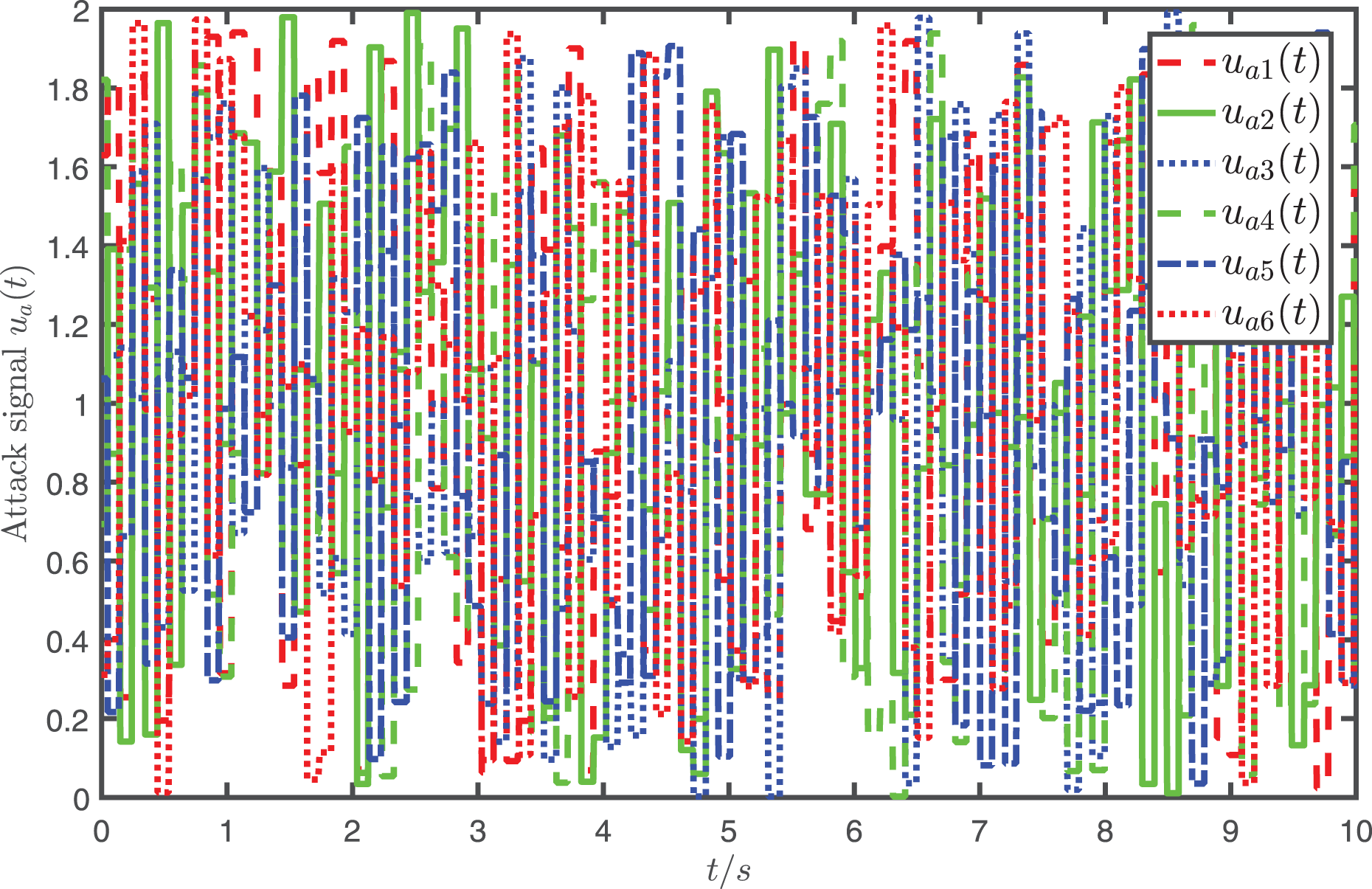
In the simulation, the parameters are specified as , , , and the attack signal is randomly selected from which is shown in Fig. 3.
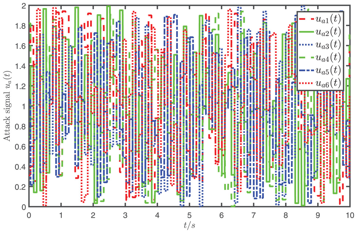
Figure 3: Profiles of the attack signal where represents the -th element of .
The system input in Eq. (44) is chosen as
(49) where is defined in Eq. (25) with , where K is chosen as
such that A + BK is Hurwitz.
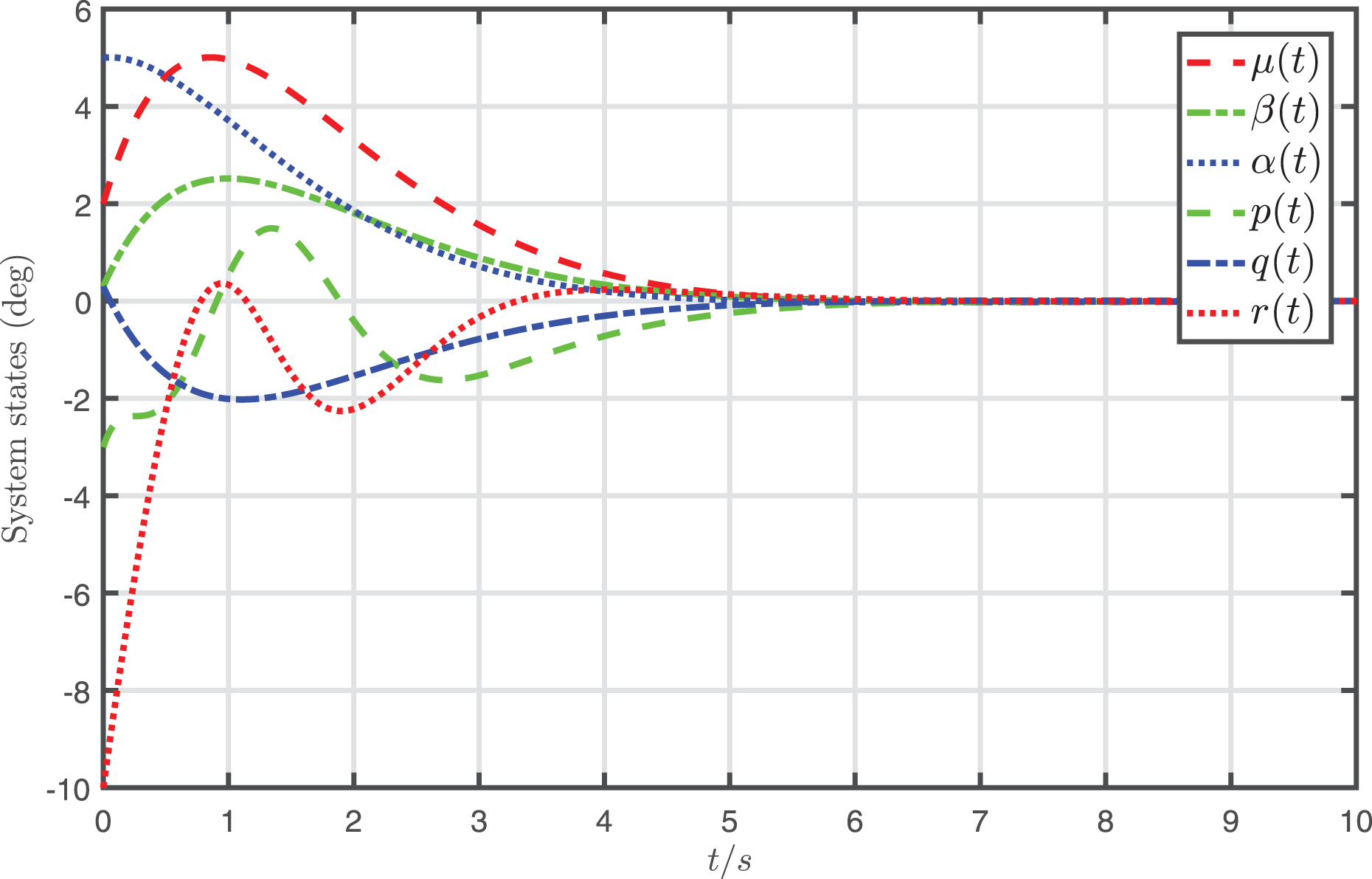
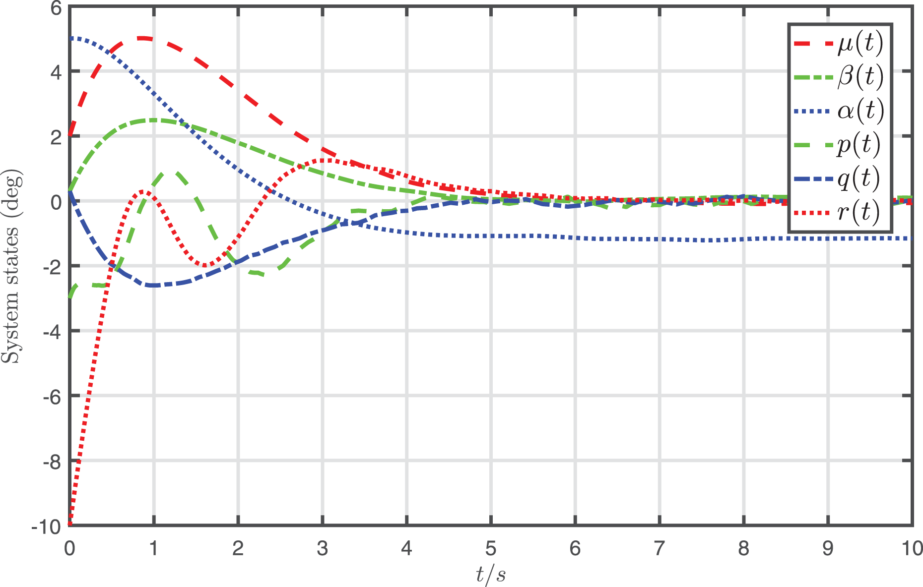
The simulation results of the nonlinear system, which is jointly controlled by the desired input and the attack-compensation input , are demonstrated in Fig. 4. In addition, the state trajectories of the nonlinear system, which is only controlled by the desired input , are depicted in Fig. 5.
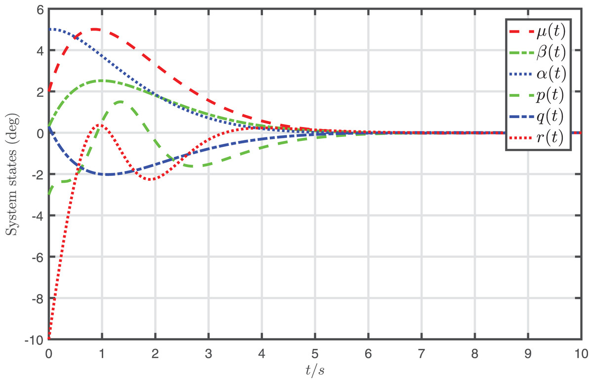
Figure 4: Profiles of system states under the desired input and the attack-compensation input .
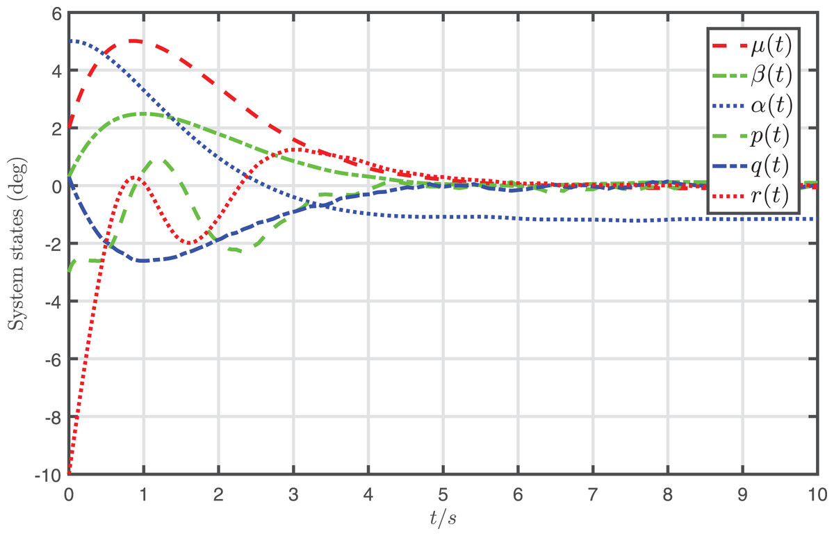
Figure 5: Profiles of system states under the desired input .
It is shown from Fig. 4 that the system states almost converge to zero when the system controlled by the proposed attack-compensation approach. On the contrary, if the desired input designed for the nominal model is applied to the system under FDI attack, the behavior of the system degrades severely, as shown in Fig. 5. The simulation results demonstrate that very satisfactory compensation performances are achieved by the proposed attack-compensation approach for the system even in the presence of the attack, and much better performances can be achieved than the desired-input-based control, which verify that the proposed attack-compensation scheme is very effective to cope with the attack.
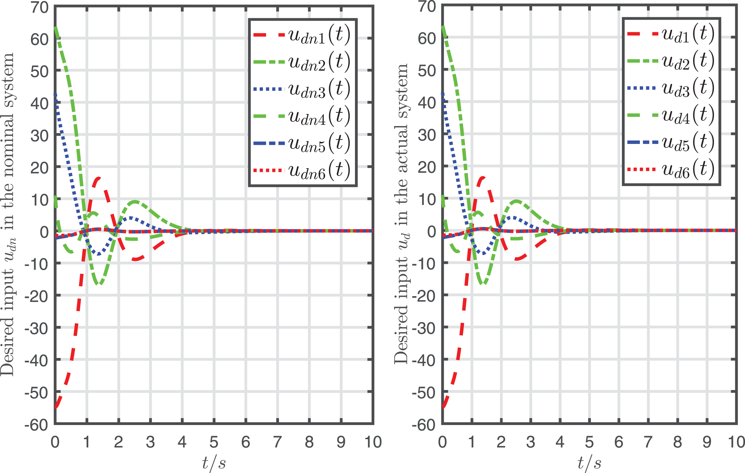
To display the effect of system recovery, the desired input and its nominal input are drawn in Fig. 6, and the actual system state and its nominal state are drawn in Fig. 7.
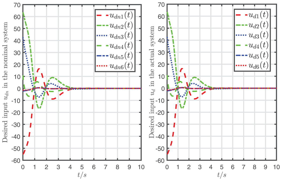
Figure 6: Desired input in the nominal system and the desired input in the actual system.

Figure 7: System states in the nominal system controlled by the desired input and the ones in the actual system controlled by the desired input and the attack-compensation input .
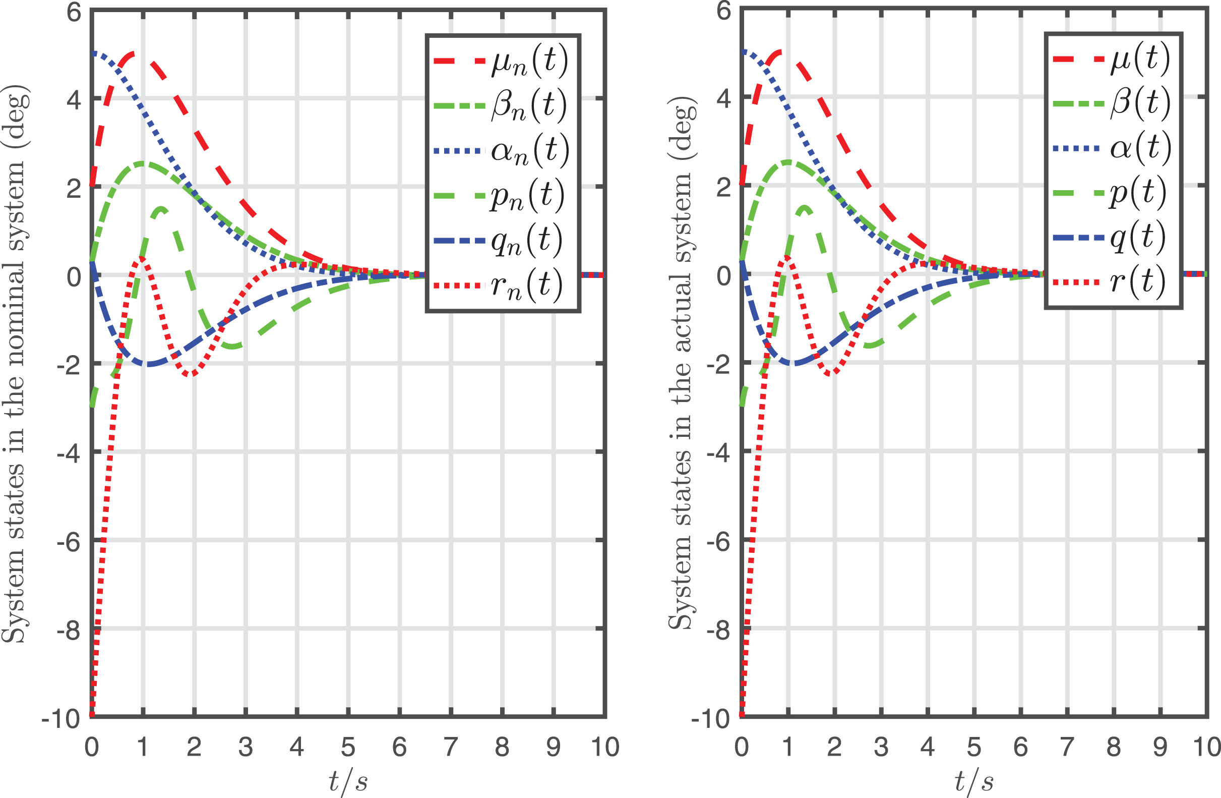
It can be seen from Figs. 6, 7 that the mapping relationship between the desired input and system states is almost the same as and in the nominal system. In other words, the system is almost fully recovered (that is because the recursive attack-compensation input signal added into the system input can almost fully compensate the attack).
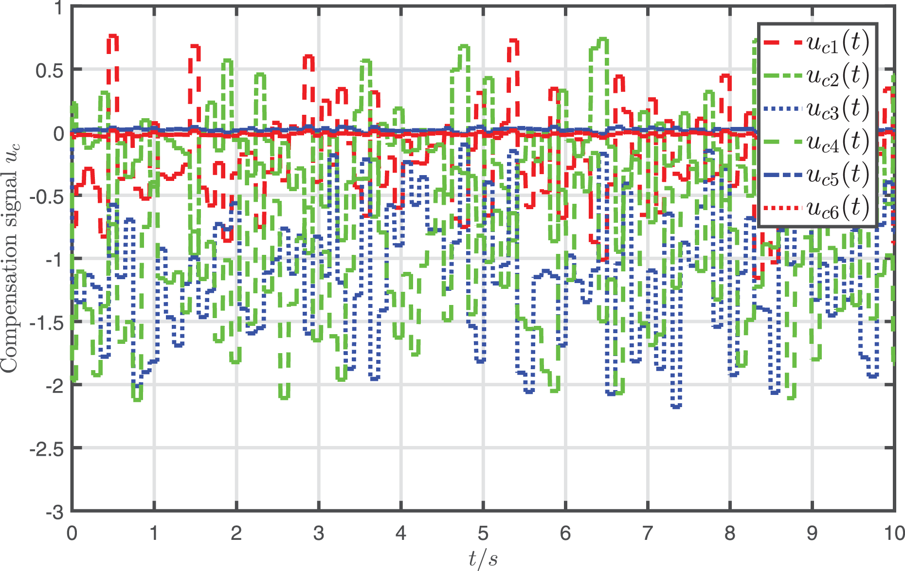
In addition, the attack-compensation input signal is presented in Fig. 8, which shows that is the same order of magnitude as the attack signal .
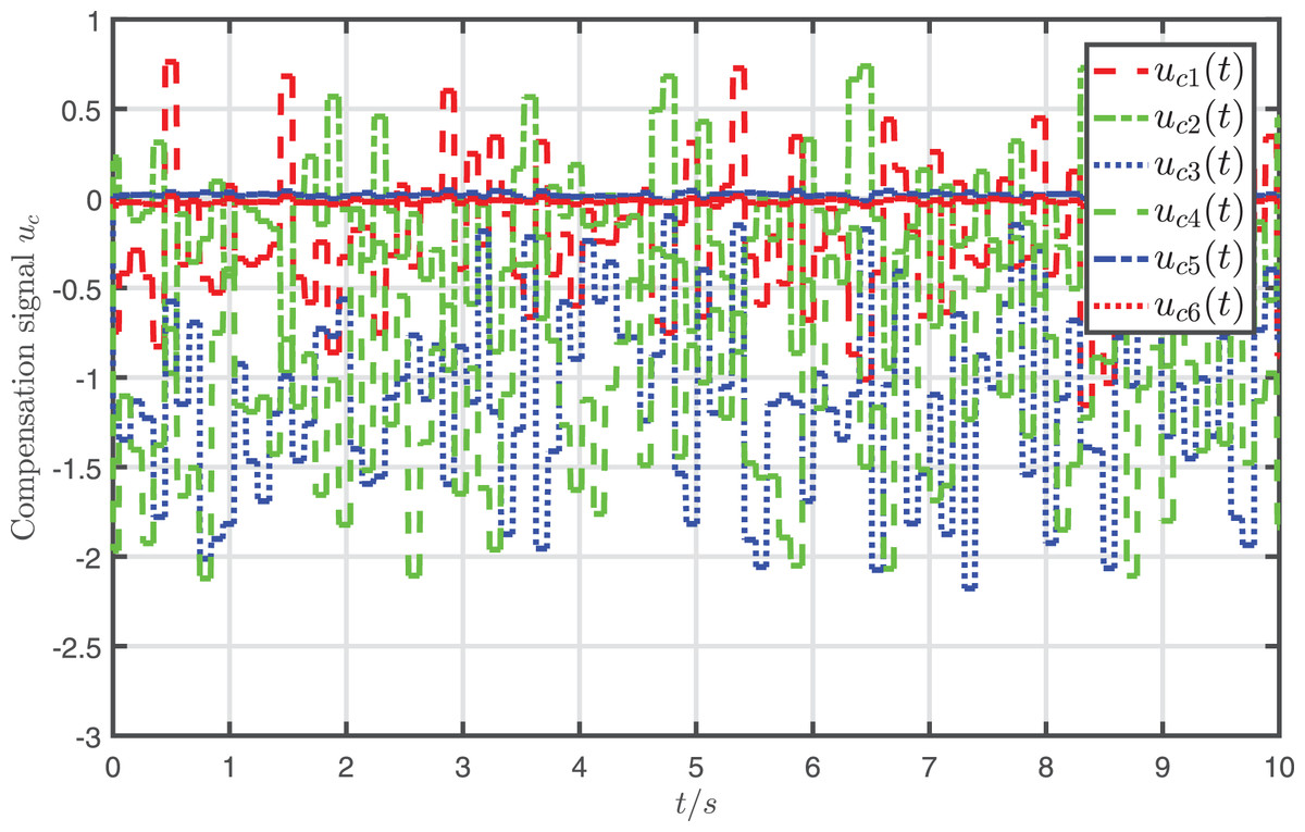
Figure 8: Profiles of compensation signal .
To provide a more intuitive and clear description of the system recovery performance of the proposed approach, the root mean squared error (RMSE) index is used. Table 2 lists the RMSE and mean absolute error (MAE) values for state deviation caused by the attack, where , , , , and . The results demonstrate that the proposed strategy achieves superior system recovery performance.
| Indices under the proposed approach | RSME of | RSME of | RSME of | RSME of | RSME of | RSME of |
|---|---|---|---|---|---|---|
| Values | ||||||
| Indices without the proposed approach | RSME of | RSME of | RSME of | RSME of | RSME of | RSME of |
| Values | 0.0026 | 0.0042 | 1.1961 | 0.2099 | 0.0358 | 0.3036 |
Conclusions
In this article, the system recovery problem has been studied for MIMO nonlinear systems under FDI attack. With the help of feedback-linearizing design technique, the nonlinear system has been transformed into a linear one. In order to obtain the system states, a high-gain approximate differentiator has been utilized. After that, a recursive attack-compensation input signal has been skillfully designed and added into the system input to almost fully recover the system. It has been proved that an upper bound of the state deviation caused by the attack is an infinitesimal of the same order as the period of the attack-compensation input signal, and thus the system can be almost fully recovered when a small enough period is selected.