
An explainable intrusion detection system using novel Indian millipede optimization and WGAN-GP with a dynamic attention-based ensemble model
- Published
- Accepted
- Received
- Academic Editor
- Markus Endler
- Subject Areas
- Artificial Intelligence, Computer Networks and Communications, Optimization Theory and Computation, Security and Privacy, Neural Networks
- Keywords
- Intrusion detection system, Cyber security, Indian millipede optimization algorithm, Ensemble learning, Dynamic-attention, Enhanced WGAN-GP
- Copyright
- © 2025 Chinnasamy and Subramanian
- Licence
- This is an open access article distributed under the terms of the Creative Commons Attribution License, which permits unrestricted use, distribution, reproduction and adaptation in any medium and for any purpose provided that it is properly attributed. For attribution, the original author(s), title, publication source (PeerJ Computer Science) and either DOI or URL of the article must be cited.
- Cite this article
- 2025. An explainable intrusion detection system using novel Indian millipede optimization and WGAN-GP with a dynamic attention-based ensemble model. PeerJ Computer Science 11:e3278 https://doi.org/10.7717/peerj-cs.3278
Abstract
In the rapidly changing field of cybersecurity, strong and efficient Intrusion Detection Systems (IDS) are essential for spotting malicious activities on the network traffic. However, traditional IDS models often face challenges such as too many irrelevant features (high-dimensional data), uneven class distributions (imbalanced datasets), and constantly evolving threats (shifting attack patterns). To overcome these issues, we introduce a hybrid framework called WGAN-GP_IMOA_DA_Ensemble. It combines: (i) a new bio-inspired Indian Millipede Optimization Algorithm (IMOA), based on the movement and foraging behavior of Indian millipedes, for selecting the most relevant features; (ii) an enhanced Wasserstein Generative Adversarial Network with Gradient Penalty (WGAN-GP) that uses attention layers, layer normalization, and skip connections in the discriminator, producing more realistic synthetic samples for rare attack types; and (iii) a dynamic attention-based ensemble, DA_Ensemble, which integrates three deep learning models namely Feedforward Neural Network (FNN), Convolutional Neural Network (CNN), and Long Short-Term Memory (LSTM), and adaptively weights their predictions in real time, emphasizing the most accurate model for a specific type of traffic. The model was tested on benchmark datasets such as UNSW-NB15, H23Q, and CIC-IDS2017 under multiclass and binary settings. In binary classification, the model achieved 100% “accuracy, precision, recall, and F1-score” on the UNSW-NB15 dataset, surpassing the best benchmark method, Optimized Hybrid Deep Neural Network + Enhanced Conditional Random Field (OHDNN+ECRF), by nearly 2%. On CIC-IDS2017 and H23Q, it attained about 99% across all four metrics, improving previous baselines by 2% to 3%. In multiclass classification, it reached 99% in all four metrics on UNSW-NB15 and CIC-IDS2017, and about 98% on H23Q, demonstrating a steady 2% to 4% improvement over current leading methods. These results, confirmed through five-fold cross-validation and ablation studies, show that the proposed approach reliably delivers statistically significant improvements in both binary and multiclass intrusion detection tasks.
Introduction
In the ever-changing landscape of cybersecurity, the robustness and flexibility of Intrusion Detection Systems (IDS) are essential for safeguarding information systems against malicious activities and sophisticated cyber threats (Kumar, 2025; Park et al., 2022). The two main techniques used in traditional intrusion detection are anomaly-based and signature-based (Park et al., 2022). Signature-based methods excel at identifying known threats because they recognize specific patterns (Chinnasamy & Subramanian, 2023). However, they cannot detect new, unknown attacks such as zero-day exploits. Additionally, anomaly-based techniques can detect unusual behavior, making them more flexible against new threats (Shankar et al., 2024; Momand, Jan & Ramzan, 2024). Nevertheless, they often generate many false alarms and have difficulty defining normal activity in a dynamic network environment (Bella et al., 2024). Furthermore, the success of these methods largely relies on the quality and completeness of the dataset used for detection, as well as the amount of training data available, which is often limited or imbalanced in real-world situations (Lee, Li & Li, 2023; Ahmed et al., 2024).
Deep Learning (DL) and Machine Learning (ML) methods are commonly employed to enhance IDS (Chinnasamy, Malliga & Sengupta, 2022). However, several ongoing challenges remain: feature redundancy, dataset imbalance, and the static nature of many ensemble approaches (Subramani & Selvi, 2023; Rajasoundaran et al., 2024).
Research gap
Despite considerable advancements, existing studies have critical limitations.
Feature Redundancy: Many systems do not remove irrelevant or overlapping features, leading to increased computational costs and overfitting. For example, Momand, Jan & Ramzan (2024) introduced Attention-Based CNN-IDS, which showed strong performance on Internet of Things (IoT) traffic with about 96% accuracy but had poor recall of less than 80% for minority classes due to a lack of feature selection.
Imbalanced Datasets: Rare attack types are consistently under-detected. Park et al. (2022) employed Generative Adversarial Networks (GANs) for data augmentation on CIC-IDS2017; however, detection of minority classes, such as infiltration attacks, remained insufficient, highlighting the limitations inherent in traditional GAN frameworks.
Static Ensemble Fusion: Current IDS frameworks often combine multiple models with fixed weighting schemes, which poorly adapt to changing network traffic. Shankar et al. (2024) proposed an approach merging optimization techniques with deep learning, but the static nature of ensemble weighting limited adaptability and caused decreased performance across diverse datasets.
Collectively, these drawbacks emphasize the importance of IDS architectures that incorporate efficient feature selection, robust data augmentation strategies, and adaptive model fusion mechanisms to enhance accuracy, recall, and particularly the detection of minority classes.
It is crucial to recognize that the examples given are illustrative; a comprehensive discussion of related works and additional supporting evidence can be found in the literature survey section.
Research hypothesis
This study hypothesizes that combining a biologically inspired feature selection method called Indian Millipede Optimization Algorithm (IMOA), an enhanced Wasserstein Generative Adversarial Network with Gradient Penalty (WGAN-GP), and a dynamic attention-based (DA)_ensemble classification model will notably enhance intrusion detection performance in terms of precision, accuracy, F1-score, and recall, especially in managing imbalanced datasets and identifying minority attack classes, compared to existing IDS approaches.
Novelty and advantages over prior work
Previous studies have independently examined GANs, ensemble deep learning, or optimization-driven feature selection, but significant limitations remain (Park et al., 2022; Shankar et al., 2024; Momand, Jan & Ramzan, 2024; Lee, Li & Li, 2023). In contrast, our contributions are threefold.
-
1.
Novel IMOA:
A first-of-its-kind bio-inspired optimizer that models the behavioral patterns of Anoplodesmus saussurii (Indian millipedes), including seasonal abundance (Usha, Vasanthi & Esaivani, 2022), obstacle avoidance (Dave & Sindhav, 2025), temperature response (Aswathy & Sudhikumar, 2022), resource utilization (Ramanathan et al., 2023), group movement (Anilkumar, Wesener & Moritz, 2022), defensive behavior (Dave & Sindhav, 2025), and mating behavior (Usha, Vasanthi & Esaivani, 2022). These behaviors are mathematically modeled to improve the exploration-exploitation balance. Unlike conventional optimization algorithms such as Genetic Algorithm (GA) (Fang et al., 2024), Particle Swarm Optimizer (PSO) (Jain et al., 2022), and Grey Wolf Optimizer (GWO) (Mirjalili, Mirjalili & Lewis, 2014), which primarily rely on predefined equations for search dynamics, IMOA introduces adaptive strategies that respond to the current state of search. These biologically inspired adaptations enhance feature selection efficiency in IDS applications, leading to improved classification performance.
-
2.
Feature-level discriminator enhancements in WGAN-GP:
While GAN-based data augmentation (Park et al., 2022; Lee, Li & Li, 2023) has been explored, our approach is the first to implement attention layers, layer normalization, and skip connections within the WGAN-GP discriminator to improve the realism of synthetic minority-class data. Unlike traditional oversampling techniques such as Synthetic Minority Oversampling Technique (SMOTE) (Meliboev, Alikhanov & Kim, 2022) or oversampling, this research gives better discrimination between real and generated samples and enhances minority class recall without overfitting.
-
3.
DA_Ensemble learning:
This research incorporates a DA_Ensemble mechanism, integrating Convolutional Neural Network (CNN), Long Short-Term Memory (LSTM), and Feedforward Neural Network (FNN) models. Unlike fixed-weight ensemble methods (Kumar, 2025; Bella et al., 2024; Rajasoundaran et al., 2024), this approach dynamically adjusts model weights in real time, ensuring more accurate predictions across diverse attack categories.
Practical benefits
Beyond theoretical novelty, the proposed framework offers several practical benefits for real-world IDS deployments, including:
-
(1)
Lightweight deployment for edge devices: The features selected through IMOA reduces computational overhead. As a result, the model becomes lightweight. So, it is appropriate for resource-limited settings such as IoT and edge devices.
-
(2)
Improved detection of rare and emerging attacks: WGAN-GP-based data augmentation ensures balanced training, which helps detect minority class attacks more effectively and improves security in critical infrastructure.
-
(3)
Context-aware decision making: The dynamic attention mechanism customizes the decision-making process to individual traffic instances, increasing accuracy in complex, real-world traffic where static models may fail.
-
(4)
Scalability across datasets: The framework is tested on diverse datasets, including CIC-IDS2017, UNSW-NB15, and H23Q. It shows robustness and flexibility across different network environments and traffic patterns.
-
(5)
Better interpretability for analysts: The attention weights can be visualized to indicate which features or base learners impacted a prediction, aiding human analysts in trust and decision justification.
-
(6)
Ablation study for model validation: Shows how each part, including IMOA, WGAN-GP, and attention-based ensemble, contributes to overall system performance, allowing users to adjust or simplify the model for specific deployment needs without significant performance loss.
-
(7)
Computational efficiency analysis: Evaluates the model’s ability to deploy in real-world scenarios, especially on resource-limited edge devices, by providing insights into time and memory usage and supporting scalability and hardware compatibility decisions.
-
(8)
Comprehensive comparison: Confirms the effectiveness of the WGAN-GP_IMOA_DA_Ensemble model across various scenarios.
The remainder of this study is arranged in the following manner: The literature review covers similar studies in the field of IDS. The materials and methods provide the details of IMOA and WGAN-GP, as well as the proposed DA_Ensemble, including the architectures of IMOA, WGAN-GP, and the ensemble models leveraged in this research. The Results section describes the experimental setup, evaluation metrics, and experiment outcomes. The Discussion section provides details of the classification report and a comprehensive comparison with benchmark datasets. Finally, the conclusion covers the summary and possible further research potential.
Literature survey
The details, such as feature selection methods, classification techniques, datasets used, advantages, and limitations of some related works, are listed in Table 1. This section offers a summary of recent research on strategies for handling high-dimensional data, addressing class imbalance in datasets, and DL based methodologies for developing effective IDS.
| Authors | Feature selection methods | Classification methods | Datasets used | Advantages | Limitations |
|---|---|---|---|---|---|
| UNSW-NB15 binary (Kareem et al., 2022) | GTO-BSA | K-NN | UNSW-NB15, CICIDS2017, NSL-KDD, BoT-IoT | Better convergence, higher accuracy. | Limited scope, high cost. |
| Turukmane & Devendiran (2024) | Modified Singular Value Decomposition (M-SvD) |
M-MultiSVM | CSE-CIC-IDS 2018, UNSWNB-15 | High accuracy, reduced imbalance. | Dataset-bound, complex model. |
| Meliboev, Alikhanov & Kim (2022) | SMOTE for balancing classes | CNN+LSTM | UNSW-NB15, KDDCup’99, NSL-KDD | Balancing the datasets significantly improved model accuracy and F-scores across all benchmarks. | Training recurrent models requires higher computation and longer epochs compared to CNN. |
| Ragab & Sabir (2022) | Poor and Rich Optimization Algorithm (PROA) for hyperparameter tuning | Hybrid CNN-ALSTM with attention mechanism | KDDCup’99, NSL-KDD, UNSW-NB15, CICIDS2017 | High accuracy, robust detection. | Complex design, dataset-dependent. |
| Altunay & Albayrak (2023) | CNN+LSTM | UNSW-NB15, X-IIoTID | High accuracy, hybrid effectiveness. | Dataset-specific, limited generalization. | |
| Thilagam & Aruna (2023) | Hybrid CNN-LSTM with AES encryption | NSL-KDD, UNSW-NB15 | Strong security, high accuracy | Complex process, dataset-limited | |
| Karthic & Kumar (2023) | Enhanced Conditional Random Field-based feature selection | Optimized Hybrid Deep Neural Network (OHDNN): Hybrid CNN-LSTM, optimized using Adaptive Golden Eagle Optimization | NSL-KDD, UNSW-NB15 | Improved accuracy, effective features. | Dataset-limited, high complexity. |
|
CIIC-IDS2017 Binary (Hanafi et al., 2023) |
IBGJO | LSTM | CICIDS2017, NSL-KDD |
High accuracy, effective feature selection. | Dataset-limited, reduced efficiency scaling. |
| Bowen et al. (2023) | Recursive Feature Elimination (RFE) | Hybrid CNN + BLSTM | CIC-IDS2017, IoT-23, Bot-IoT, UNSW-NB15 | Strong detection, hybrid effectiveness | Dataset-dependent, misses rare attacks |
| Li, Li & Li (2023) | GAN for data augmentation, CNN-BiLSTM with self-attention mechanism | CIC-IDS2017 | Handles imbalance, higher accuracy | High complexity, dataset-specific | |
| Vishwakarma & Kesswani (2023) | Naïve Bayes and Elliptic Envelope | NSL-KDD, UNSW-NB15, CIC-IDS2017 | High accuracy, efficient detection. | Multi-phase complexity, dataset-bound. | |
| Chinnasamy, Subramanian & Sengupta (2023a) | HBO | ANN | CIC-IDS2017 | Efficient feature selection | Dataset limited, class imbalance issue |
|
UNSW-NB15 multiclass (Bakro et al., 2024) |
Grasshopper Optimization Algorithm (GOA) and GA | Random Forest classifier | UNSW-NB15, CIC-DDoS2019, CIC Bell DNS EXF 2021 | High accuracy, improved feature selection | Complex process, high computation |
| Sayegh, Dong & Al-madani (2024) | Correlation-Based Feature Selection (CFS) Recursive Feature Elimination (RFE) |
Random Forest (RF) Support Vector Machine (SVM), K-Nearest Neighbor (KNN), Naïve Bayes (NB), Decision Tree (DT) |
UNSW-NB15 | Improved detection, handles imbalance | Oversampling risks, dataset-specific |
| Sajid et al. (2024) | Principal Component Analysis (PCA) and Information Gain (IG) | Random Forest (RF) Gradient Boosting Machine (GBM), Logistic Regression (LR), Naïve Bayes (NB), Decision Tree (DT), K-Nearest Neighbors (KNN) |
UNSW-NB15 | High detection, low FAR | Complex design, dataset-dependent |
| More et al. (2024) | Correlation Analysis and Random Sampling | Logistic Regression, Decision Tree | UNSW-NB15 | Better accuracy, improved evaluation | Dataset-specific, limited generalization |
| Yin et al. (2023) | Random Forest Importance, Recursive Feature Elimination (RFE) | MLP with two hidden layers | UNSW-NB15 dataset | Reduced features, improved accuracy | Dataset-limited, modest gains |
|
CIC-IDS2017 multiclass (Yao, Shi & Zhao, 2023) |
Bidirectional GAN (BiGAN) with Wasserstein distance, Fog-Cloud joint training | UNSW-NB15, CIC-IDS2017 | Scalable detection, reduced false alarms | Complex training, dataset-limited | |
| Bacevicius & Paulauskaite-Taraseviciene (2023) | Logistic Regression, Decision Trees | CIC-IDS2017, CSE-CIC-IDS2018 | Strong multi-class performance, interpretable results | Imbalance persists, dataset-specific | |
| Aljehane et al. (2024) | Golden Jackal Optimization Algorithm (GJOA) | Attention-based bi-directional long short-term memory (A-BiLSTM) | CIC-IDS2017 | Better accuracy, optimized feature selection | High complexity, dataset-specific |
| Ahmed et al. (2024) | Consensus Hybrid Ensemble Model (CHEM): Voting-based ensemble with RF, DT, XGBoost, MLP | Kdd99, NSL-KDD, CIC-IDS2017, BoTNeTIoT, Edge-IIoTset | Adaptive, interpretable, strong accuracy | Complex ensemble, high computation | |
| Aktar & Nur (2023) | Deep Contractive Autoencoder (DCAE) with stochastic threshold selection | CIC-IDS2017, NSL-KDD, CIC-DDoS2019 | High accuracy, effective anomaly detection | Dataset-limited, high training cost | |
| H23Q dataset (multiclass classification) (Chatzoglou et al., 2023) | Shallow and deep learning techniques (various ML models) | H23Q Dataset | New dataset, real attack coverage | Early stage, limited scope |
Handling high-dimensional data
IDS datasets are often high-dimensional, which may include noise, redundant, and irrelevant information (Chinnasamy, Malliga & Sengupta, 2022). Dimensionality reduction and feature selection are approaches employed to handle the problems related to high-dimensional data and reduce the computational complexity, improve the accuracy, and avoid overfitting (Ahmed et al., 2024; Fang et al., 2024; Meliboev, Alikhanov & Kim, 2022).
Kareem et al. (2022) proposed GTO-BSA framework that integrates “Gorilla Troops Optimizer” (GTO) and “Bird Swarm Algorithm” (BSA), using K-Nearest Neighbour for classification, achieving up to 98.7% accuracy on four datasets. GTO-BSA relies on two metaheuristics, increasing complexity and limiting scalability for large datasets. It doesn’t address data imbalance or adaptive classification, restricting use in dynamic environments. In contrast, the WGAN-GP_IMOA_DA_Ensemble framework uses IMOA-based feature selection, which retains discriminative features with lower computational overhead. It integrates data augmentation with enhanced WGAN-GP and adaptive ensemble fusion to address redundancy, imbalance, and adaptability within a unified framework.
Turukmane & Devendiran (2024) designed a hybrid IDS that uses “Advanced Synthetic Minority Oversampling Technique” (ASmoT) to tackle the problem of class imbalance. Additionally, feature extraction is performed by “Modified Singular Value Decomposition” (M-SVD). Later, essential features are identified using “Opposition-based Northern Goshawk Optimization algorithm” (ONgO). The system employs a “Mud Ring assisted multilayer support vector machine” (M-MultiSVM) classifier. The performance assessment is done by utilizing the CIC-IDS 2018 and UNSW-NB15 datasets. While effective, the pipeline is computationally demanding and lacks detailed analysis of minority-class detection or ablation to determine which modules contribute most to performance. In contrast, the WGAN-GP_IMOA_DA_Ensemble framework uses WGAN-GP for realistic data balancing and a dynamic attention-based ensemble to provide both adaptability and explainability.
Hanafi et al. (2023) introduced a hybrid IDS model called IBGJO-LSTM, where the essential features are identified by the improved Binary Golden Jackal Optimization (IBGJO). Then, the classification is done by LSTM, which is optimized through opposition-based learning (OBL) to avoid local optima. NSL KDD and CICIDS2017 datasets are utilized to assess the performance. It does not address class imbalance or the adaptive fusion of multiple learners. Our approach instead provides feature selection, imbalance handling, and dynamic attention for the explainability of the framework.
Chinnasamy, Subramanian & Sengupta (2023a) designed an IDS model that utilizes the honey badger optimization algorithm (HBO) to identify the essential features. Additionally, the classification is conducted by the Artificial Neural Network (ANN). But the system was evaluated using only one dataset and doesn’t tackle the class imbalance problem. In contrast, our approach tests the framework on CIC-IDS2017, H23Q, and UNSW-NB15 datasets, tackles the problem of class imbalance with WGAN-GP, and provides explainability through dynamic attention.
Bakro et al. (2024) designed an IDS for the cloud where feature selection is performed using a hybrid bio-inspired method that combines GOA and GA. A Random Forest classifier trained on these features was tested on CIC Bell DNS, CIC-DDoS2019, and UNSW-NB15 datasets. The framework does not explicitly address class imbalance or offer mechanisms for adaptive integration of multiple learners. The proposed model mitigates these limitations by using IMOA for lightweight feature selection, WGAN-GP to balance classes, and a DA_Ensemble to enhance scalability and generalization across diverse attack scenarios.
Aljehane et al. (2024) proposed a GJOADL-Intrusion Detection System for Network Security (IDSNS) model, where the most relevant features are identified by the Golden Jackal Optimization Algorithm (GJOA). Then, the classification is performed with Attention-based Bidirectional Long Short Term Memory (A-BiLSTM). Besides, hyperparameter tuning is performed by the SSA. However, the model didn’t tackle the class imbalance problem. The proposed framework directly addresses the class imbalance issue by leveraging WGAN-GP to produce synthetic minority class instances, ensuring balanced training and improved detection across both majority and minority attack classes.
In summary, researchers have used various bio-inspired optimization algorithms for identifying the essential features and have employed either ML or DL models for classification. The feature selection methods tackle the problems of high-dimensional data.
Handling imbalanced data
During IDS development, the dataset has an uneven distribution between attack and benign classes. Managing this imbalance remains essential. Researchers have suggested different methods to deal with the problem of class imbalance.
Meliboev, Alikhanov & Kim (2022) discussed how class imbalance in intrusion detection datasets may cause low performance, especially in identifying minority attacks. The SMOTE technique has been used to balance the data. Moreover, DL models like LSTM and CNN performed significantly better on the balanced datasets compared to the imbalanced ones. However, the framework did not address the high-dimensionality problem and lacked interpretability in its results. In contrast, the proposed WGAN-GP_IMOA_DA_Ensemble addresses the high-dimensionality problem through feature selection with IMOA and offers interpretability in results with dynamic attention.
Park et al. (2022) utilized a Boundary Equilibrium Generative Adversarial Network (BEGAN) with Wasserstein distance for generating synthetic instances for minority attack classes. Constantin et al. (2024) evaluated various GAN models, like energy-based, Wasserstein, gradient penalty, LSTM-GAN, and conditional on traffic data from 16 users, with results demonstrating improved performance of intrusion detection models.
Kumar & Sinha (2023) employed a Wasserstein Conditional Generative Adversarial Network (WCGAN) with a gradient penalty to produce synthetic attack instances for underrepresented classes. In addition, the synthetic samples were combined with the real data and evaluated with the XGBoost classifier. Jamoos et al. (2023) developed a GAN-based model, named Temporal Dilated Convolutional Generative Adversarial Network (TDCGAN), for producing synthetic instances for minority attack classes in the UGR’16 dataset. By integrating three discriminators and an election mechanism, the model ensures high-quality data generation, leading to improved detection accuracy, precision, and recall. Cai et al. (2023) suggested an IDS framework named the CycleGAN Self Attention-Recurrent Neural Network (CGSA-RNN), which enhances attack detection by addressing data imbalance through an improved CycleGAN, which performs data augmentation using style transfer. By integrating a self-attention mechanism and replacing Rectified Linear Unit (ReLU) with LeakyReLU in the CycleGAN generator, the model reduces image distortion and captures critical features more effectively. Alsirhani et al. (2023) developed a DL-based IDS that utilizes Deep Convolutional GAN (DCGAN) for data augmentation to handle the issue of imbalance in datasets. By producing realistic synthetic samples of minority attack classes, the model significantly improved detection accuracy and robustness.
Although many GAN-based methods, such as WCGAN (Kumar & Sinha, 2023), BEGAN (Park et al., 2022), DCGAN (Alsirhani et al., 2023), TDCGAN (Jamoos et al., 2023), and CycleGAN (Cai et al., 2023), successfully mitigate class imbalance by generating synthetic samples, they do not incorporate feature selection algorithms, which may lead to redundant or irrelevant features that degrade performance. Moreover, these approaches lack explainability mechanisms, making it difficult to interpret or trust the decisions of the IDS models in critical security contexts. As a result, they remain limited in practical deployment despite achieving improved accuracy on benchmark datasets.
The proposed WGAN-GP_IMOA_DA_Ensemble addresses these gaps by using IMOA for effective feature selection, reducing dimensionality, and improving detection efficiency, while the dynamic attention ensemble enhances interpretability by highlighting feature contributions. Additionally, WGAN-GP ensures balanced training data, allowing the model to achieve both high accuracy and explainability in real-world IDS.
Srivastava, Sinha & Kumar (2023) suggested an IDS using WCGAN-GP for realistic data augmentation and GA for feature selection to address data imbalance. The model, combined with a Boost classifier, outperformed traditional and state-of-the-art methods by generating high-quality synthetic samples and optimizing features. The framework did not address interpretability. In contrast, the proposed WGAN-GP_IMOA_DA_Ensemble approach introduces interpretability through a dynamic attention-based ensemble.
Deep learning-based classification
Recently, DL methods have been employed for classification tasks in developing effective IDS. Meliboev, Alikhanov & Kim (2022) explored DL architectures, including CNN, LSTM, Recurrent Neural Network (RNN), and Gated Recurrent Unit (GRU), for identifying intrusion by analyzing sequential network traffic data. Among the models tested, CNN and the CNN-LSTM hybrid performed better. However, it did not address the issue of high dimensionality. The proposed WGAN-GP_IMOA_DA_Ensemble framework introduces feature selection through IMOA and reduces dimensionality.
Altunay & Albayrak (2023) designed an IDS for Industrial IoT (IIoT) by integrating CNN and LSTM architectures to enhance threat identification. Although tested on two datasets, the model only utilized classification with basic preprocessing methods. It didn’t address issues like high dimensionality, data imbalance, and model interpretability. In contrast, the proposed WGAN-GP_IMOA_DA_Ensemble framework introduces feature selection through IMOA, which reduces dimensionality, handles class imbalance with WGAN-GP by producing realistic samples of minority attack instances, and provides interpretability through dynamic attention.
Thilagam & Aruna (2023) proposed an IDS for cloud computing environments by integrating an Lion Mutated-Genetic Algorithm (LM-GA) and a hybrid CNN-LSTM DL model. The LM-GA optimizes encryption keys for securing non-intruded data using AES encryption, while the CNN-LSTM model effectively detects intrusions by analyzing preprocessed and balanced input data. The system did not address the issue of model interpretability. In contrast, our proposed system offers model interpretability through dynamic attention.
Karthic & Kumar (2023) designed an IDS where the essential features are identified using an enhanced Conditional Random Field. Additionally, an Optimized Hybrid DeepNeural Network (OHDNN) is employed for classification. This approach focuses on performance but did not address the explainability of results and class imbalance problems. The proposed system offers interpretability through dynamic attention and utilizes WGAN-GP to tackle the class imbalance.
Li, Li & Li (2023) introduced a GAN-CNN-BiLSTM model to enhance network intrusion detection by addressing data imbalance with GAN for data augmentation and combining CNN with Bidirectional LSTM, called BiLSTM networks for classification. However, they didn’t address the problem of a high-dimensional dataset. Our proposed system addresses this limitation with IMOA-based feature selection.
Attention mechanism
In IDS, attention mechanisms enhance DL models by enabling them to concentrate on the essential parts of network traffic instances (Ragab & Sabir, 2022). This selective focus allows the models to assign higher importance to critical features indicative of malicious activity, thereby reducing false positives and improving detection accuracy. However, the class imbalance issue and problems of high dimensionality, which lead to computational overhead, persist. The proposed system overcomes these limitations with IMOA-based feature selection and WGAN-GP-based synthetic data generation.
Aljehane et al. (2024) developed an IDS that utilizes Attention-based BiLSTM (A-BiLSTM) to improve the capability of the model to focus on critical temporal patterns in intrusion samples. The system fails to handle the class imbalance issue. The suggested approach addresses the class imbalance problem through WGAN-GP-based synthetic data generation.
Ahmed et al. (2024) employed a random oversampling technique to overcome the class imbalance issue. Besides, the model provides interpretability through “Shapley Additive explanations” (SHAP) and “Local Interpretable Model-agnostic Explanations” (LIME). However, it did not address the high dimensionality issue. The proposed WGAN-GP_IMOA_DA_Ensemble addresses the high dimensionality issue through IMOA-based feature selection.
In summary, recent advancements in IDS have utilized bio-inspired optimization algorithms for feature selection, GAN-based frameworks for addressing data imbalance, and DL models for classification. Notably, the integration of attention mechanisms has further contributed to the overall improvement in performance by making them focus on critical features of network traffic, enhancing detection precision, and reducing false positives.
From the detailed study of the previous literature, the general block diagram for the development of an IDS is designed and is shown in Fig. 1. It has been observed that the AI-based IDS generally preprocesses the dataset, such as data cleaning, normalization, and scaling (Devendiran & Turukmane, 2024). Next, some optimization algorithms identify the essential features of the dataset. Then, the dataset is divided into training and test datasets. Later, the classification model is trained with the training dataset. Finally, the framework’s effectiveness is evaluated using performance metrics.
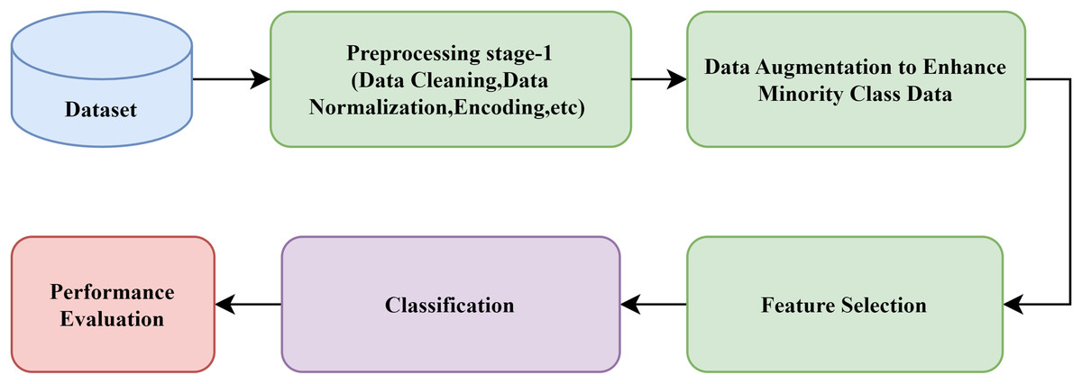
Figure 1: General block diagram of a typical IDS.
Materials and Methods
This section provides the details of the suggested model, including the IMOA algorithm, WGAN-GP algorithm, dataset preprocessing, proposed WGAN-GP_IMOA_DA_Ensemble model, and the dynamic attention mechanism. The source code for this research can be accessed at https://doi.org/10.5281/zenodo.17153877.
Novel Indian millipede optimization
A technique for finding the best solution to a problem from a set of possible solutions is known as an optimization algorithm (Nandhini & SVN, 2024). These algorithms are designed for maximizing or minimizing an objective function by iteratively improving candidate solutions (Devendiran & Turukmane, 2024).
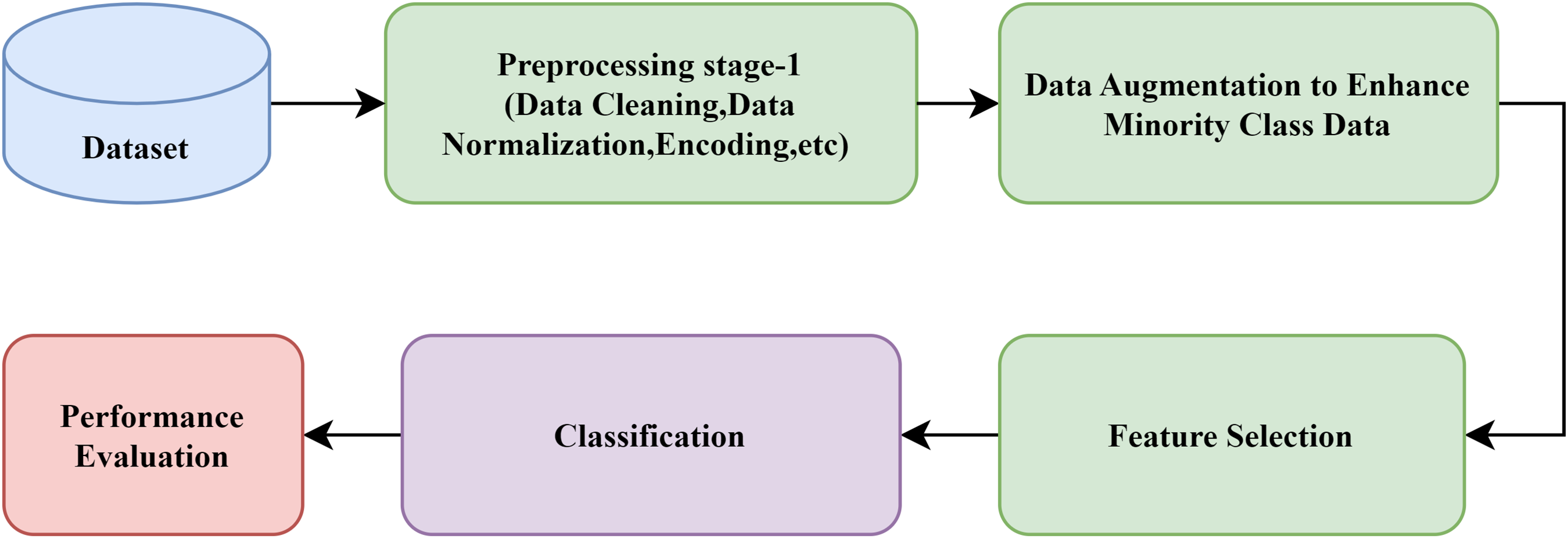
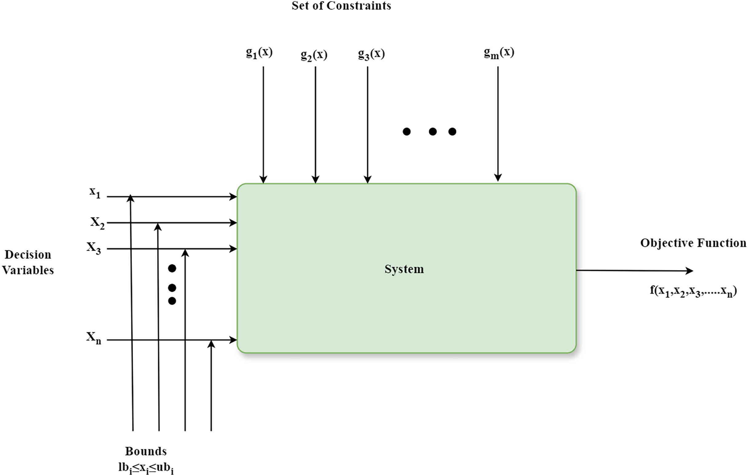
The schematic diagram that shows the components of an optimization algorithm is depicted in Fig. 2. Firstly, it has a parameter named decision variable x1, x2, …, xn that can be fine-tuned for identifying an optimal solution to a problem. Secondly, the limits on decision variables, known as bounds lbi ≤ xi ≤ ubi, define the feasible region within the search space. Next, constraints g1(x), g2(x), …, gm(x) are requirements that a solution must fulfill. Finally, a mathematical expression known as an objective function f(x1, x2, …, xn) assesses the quality of a solution by taking into account the decision variables (Otair et al., 2022). The optimization algorithms are classified broadly into traditional and metaheuristic algorithms. Metaheuristic optimization algorithms are more straightforward to comprehend and implement in comparison with conventional optimization algorithms (Jia et al., 2023). The metaheuristic optimization process finds the optimal solution xbest after numerous iterations. It yields a new solution xnew {x1, x2, …xn} in every iteration. If xnew is superior to xbest, then xbest is updated to xnew. The iterations persist until the discovered solution fulfills specific predefined criteria. The last solution is the optimal or best solution (Jia et al., 2023). Despite the numerous meta-heuristic algorithms developed in recent years, as per the No Free Lunch theorem, there is no single algorithm that can solve every problem (Fraihat et al., 2023). An algorithm that performs exceptionally well for one problem may not achieve the same effectiveness for other issues.
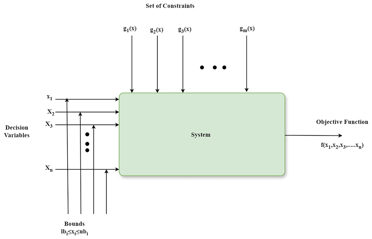
Figure 2: Fundamental components of the optimization algorithm.
In this article, a novel IMOA that mimics the behavior of the Indian millipede is proposed for identifying the crucial features in the very large dataset.
Indian millipede general biology
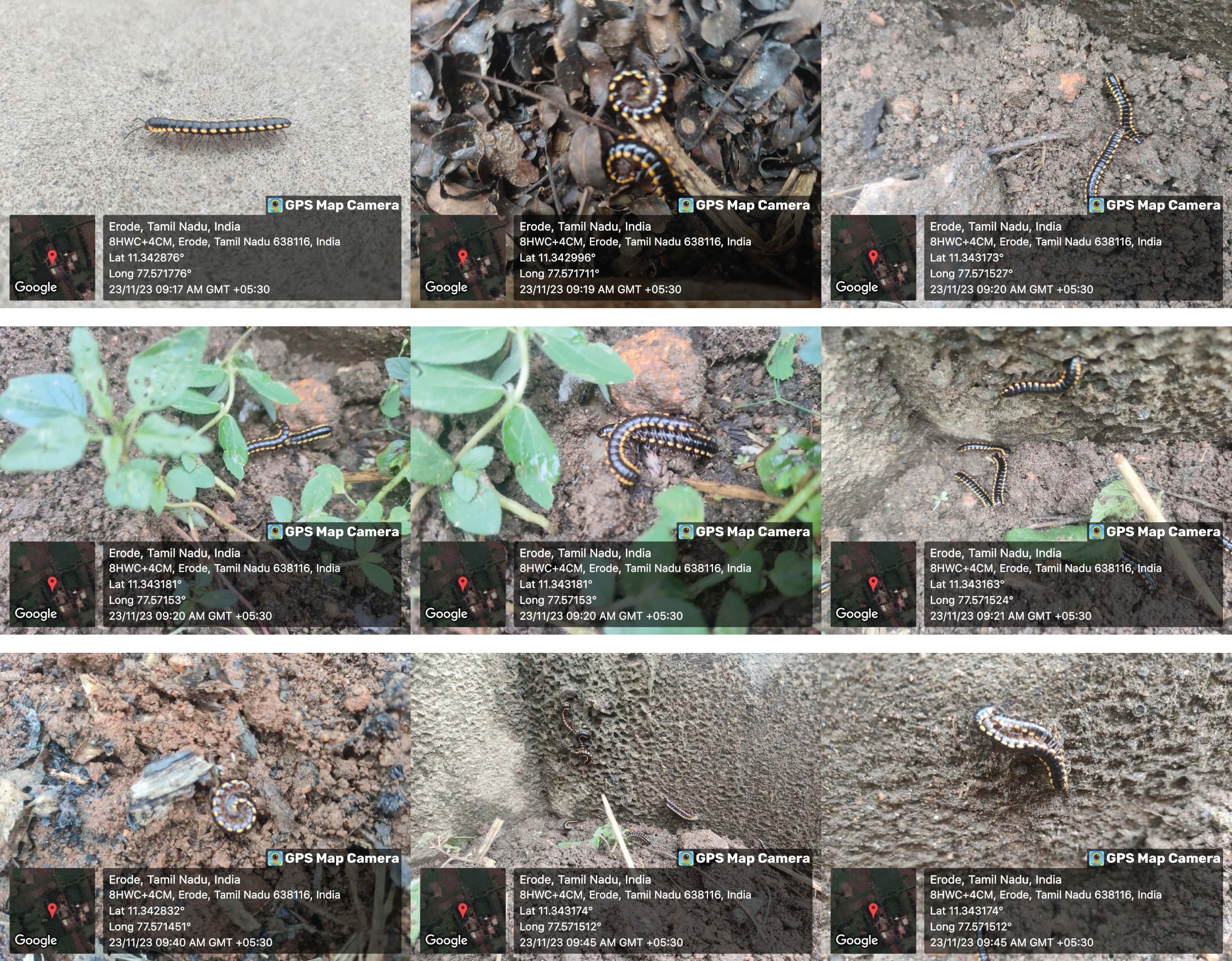
The millipedes are specialists of the soil, which can be found on the ground, in the soil, among leaf litter, or in shallow subterranean environments (Ramanathan et al., 2023). They are primarily found in the tropics and subtropics of the world because they are adapted to exist in humid environments with mild temperatures. With a length of about 21–33 mm, the adult millipede is black or dark brown. They are primarily herbivores, although they also consume wood, rotting fish, and cow dung in addition to any decaying and rotting leaves and vegetable pieces (Aswathy & Sudhikumar, 2022). Figure 3 illustrates different species of Indian millipedes along with their activities such as movement, mating, and defensive behaviors. These natural behaviors serve as the biological foundation of our proposed IMOA. The most notable behavior of millipedes that can be modelled for optimization is as follows.
-
Seasonal Abundance: Millipedes are more active during the rainy season (Usha, Vasanthi & Esaivani, 2022), which can be modelled to increase exploration during certain phases (Jia et al., 2023).
-
Obstacle Avoidance: When encountering obstacles, millipedes curl up and wait before changing direction (Anilkumar, Wesener & Moritz, 2022), which can be used to avoid local optima (Otair et al., 2022).
-
Temperature Response: Millipedes seek shady areas when temperatures are high (Aswathy & Sudhikumar, 2022), analogous to moving towards better solutions in high-stress scenarios (Jia et al., 2023).
-
Resource Utilization: Millipedes prefer areas rich in organic material (Aswathy & Sudhikumar, 2022), representing the focus on high-quality solutions (Nandhini & SVN, 2024).
-
Group Movement: Millipedes move in groups (Dave & Sindhav, 2025), indicating cooperative behavior in the algorithm (Devendiran & Turukmane, 2024).
-
Defensive Behavior: Millipedes emit a foul odor when threatened (Dave & Sindhav, 2025), analogous to penalizing poor solutions (Alsirhani et al., 2023).
-
Mating Behavior: Millipedes mate by stacking (Usha, Vasanthi & Esaivani, 2022), representing crossover operations (Jia et al., 2023).
-
Predator Avoidance: Millipedes are avoided by predators due to their odor (Dave & Sindhav, 2025), which can be used to maintain diversity by reinitializing specific populations (Jia et al., 2023).
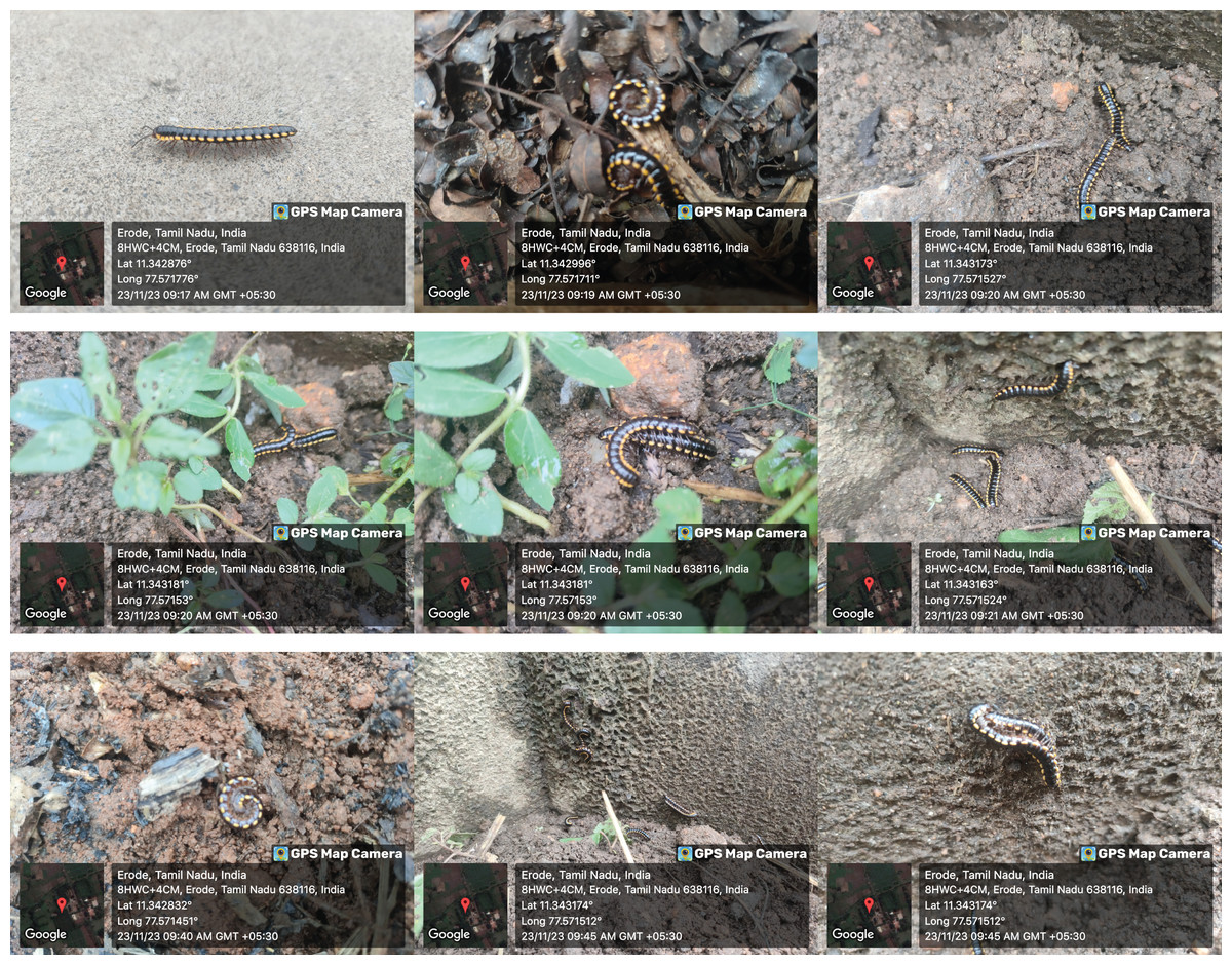
Figure 3: Composite image showcasing varied behavioral expressions of the Indian millipede.
Inspiration
IMOA is inspired by the seasonal abundance, group movement, predator avoidance, temperature response, resource utilization, defensive behavior, and mating behavior of Indian millipedes (Usha, Vasanthi & Esaivani, 2022; Dave & Sindhav, 2025; Aswathy & Sudhikumar, 2022; Ramanathan et al., 2023; Anilkumar, Wesener & Moritz, 2022). In this, the seasonal abundance, group movement, and predator avoidance correspond to the exploration phase. On the other hand, temperature response, resource utilization, defensive behavior, and mating behavior correspond to the exploitation phase of IMOA.
Mathematical model
This section gives the mathematical equivalence of the IMOA, which simulates various behaviors of the millipedes.
Algorithmic steps
IMOA is a global optimization technique since it has the potential to include both exploration and exploitation stages. The stepwise procedure of the IMOA, adapted for feature selection in IDS, is presented in Algorithm 1.
| Input: Population size N, Maximum iterations T, Temperature threshold Tth |
| Parameters: α (seasonal activity factor), β (reversal factor), γ (learning rate), |
| δ (step size), ε (social factor), λ (penalty coefficient), η (crossover coefficient) |
| Output: Best solution found |
| 1. Initialize population P with N millipedes at random positions |
| 2. Evaluate the fitness of each millipede using the objective function f(x). |
| • If constraints are violated → apply a penalty using the coefficient λ. |
| 3. Set iteration counter . |
| 4. While (t < T and not converged) do |
| 4.1. for each millipede i in P do |
| • Seasonal Abundance: update position using periodic factor (Eqs. (4) and (5)). |
| • Obstacle Avoidance: if an obstacle is detected, apply a reversal update (Eq. (6)). |
| • Temperature Response: if Temperature > Tth, move towards best-known position (Eq. (7)). |
| • Resource Utilization: refine position using local gradient (Eq. (8)). |
| • Group Movement: move towards the population mean (Eq. (9)). |
| • Defensive Behavior: apply a penalty if poor conditions are encountered (Eq. (10)). |
| • Mating Behavior: generate offspring via crossover with another individual (Eq. (11)). |
| • Predator Avoidance: if population diversity < threshold, reinitialize to a random position (Eq. (12)). |
| 4.2. Evaluate new positions and compute fitness for all millipedes (Eq. (13)). |
| • Apply a penalty if constraints are violated (Eq. (14)). |
| 4.3. Update the best solution found so far (Xbest). |
| 4.4. Increment iteration counter (t = t + 1) (Eq. (16)). |
| 5. Return the best solution Xbest. |
The detailed steps of the suggested IMOA algorithm are given below.
Step 1: Initialization
The initialization step of IMOA begins with creating an initial population of millipedes, each positioned randomly within the defined bounds of the search space. It aims to cover a wide range of the search space, which in turn promotes diversity and enhanced exploration. The detailed initialization is as follows.
-
•
Define the Bounds of the Search Space:
Each dimension j of the search space has a lower bound lbj = xmin,j and an upper bound ubj = xmax,j.
-
•
Generate Initial Positions:
For each millipede i and dimension j, generate a random position within the bounds.
Initialization for the entire population is given by Eq. (1).
(1) where P is the candidate solution
N is the number of millipedes (population size),
d is the dimensionality of the search space,
Xi is the position vector of the ith millipede.
The initial position for each millipede i in each dimension j is given by the following Eq. (2).
(2) where rand(0, 1) is a random number uniformly distributed between 0 and 1.
Also set algorithm parameters, population size N, maximum iterations T, temperature threshold Tth, and scaling factors α, β, γ, δ, ε, λ, and η.
Step 2: Fitness Evaluation
The initial fitness evaluation in IMOA involves defining the fitness function, computing the fitness for each millipede, and applying penalties for constraint violations if necessary. This process provides the initial quality assessment of the solutions, guiding the optimization process in subsequent iterations. Let be the position vector of the ith millipede,
) be the fitness function applied to ,
λ be the penalty coefficient for constraint violations, and
) be a constraint violation function that returns a positive value if constraints are violated and zero otherwise.
The penalized fitness function is given by Eq. (3).
(3) Step 3: Iterative Process
The iterative process in the IMOA includes (i) updating the positions of millipedes based on their behaviors, (ii) evaluating their fitness, and (iii) checking for convergence. This section explains in detail he iterative procedure and its mathematical equivalents.
Iterative Loop
Set the iteration counter t = 0
For each iteration until convergence:
• Update positions based on various behaviors.
• Evaluate the fitness of new positions.
• Apply penalty for constraints (if any).
• Check for convergence.
Iterative steps
Iterative step1: Seasonal Abundance
During the rainy season, Indian millipedes experience a significant increase in activity and population (Aswathy & Sudhikumar, 2022). This trait allows increased exploration. The mathematical equivalence for the seasonal abundance for more exploration is given in Eqs. (4) and (5).
(4)
(5) where α is the scaling factor, t is the current iteration, T is the maximum number of iterations, and is the random vector.
Iterative step 2: Obstacle Avoidance
When it encounters an obstacle, the Indian millipede curls up and waits for some time. Afterwards, it changes its direction (Aswathy & Sudhikumar, 2022). This is equivalent to reversing the search when there is a poor fitness to avoid local optima trapping. The mathematical equivalence of obstacle avoidance is given in Eq. (6).
(6) where is the reversal factor.
Iterative step 3: Temperature Response
Millipedes move to cooler areas when temperatures rise above 26 °C. It is analogous to moving towards better solutions in high-stress situations. The mathematical equivalence of temperature response is given in Eq. (7). Move towards better solutions xbest, if the temperature exceeds the threshold Tth.
(7) where γ is the learning rate and is the best position found so far.
Iterative step 4: Resource Utilization
Indian millipedes utilize resources efficiently by seeking out areas with abundant degradable leaves and mud. This behavior allows them to thrive in environments rich in organic matter, ensuring their survival and growth (Usha, Vasanthi & Esaivani, 2022). This behavior can be modelled as focusing on high-fitness areas. The mathematical equivalence of resource utilization is given in Eq. (8).
(8) where δ is a step size and ) is the gradient of the fitness function.
Iterative step5: Group Movement
Indian millipedes travel in clusters and exhibit group movement, enhancing their chances of finding resources and protection (Usha, Vasanthi & Esaivani, 2022). This collective behaviour helps them navigate their environment more effectively and increases their overall survival rate. This simulates the cooperative behaviour that involves multiple agents working together and sharing information to explore the search space more effectively and improve the chances of finding optimal solutions. The mathematical equivalence of group movement is given in Eq. (9).
(9) where is a social factor.
Iterative step 6: Defensive Behavior
Indian millipedes display defensive behavior by emitting a foul odor when threatened, deterring predators and ensuring their safety. This chemical defense mechanism is crucial for their survival, as it makes them unappealing to potential threats. This can be modelled as penalizing poor solutions. The mathematical equivalence of defensive behavior is given by the penalized fitness function in Eq. (10).
(10) where, λ is a penalty coefficient.
Iterative step 7: Mating Behavior
Indian millipedes exhibit mating behavior where one millipede climbs on top of another, facilitating reproduction. This behavior is crucial for the continuation of their species and helps maintain their population in suitable environments (Usha, Vasanthi & Esaivani, 2022). It represents crossover or recombination. This process involves combining parts of two or more parent solutions to create new offspring solutions, promoting genetic diversity and enhancing the search for optimal solutions. The mathematical equivalence of mating behavior is given in Eq. (11).
(11) where is a crossover coefficient.
Iterative step 8: Predator Avoidance
Indian millipedes avoid predators by emitting a foul odor, making them unappealing to birds and other animals. This chemical defense strategy is highly effective, as it deters potential threats and ensures their safety (Usha, Vasanthi & Esaivani, 2022). It can be modelled to reinitialize specific populations to avoid premature convergence and maintain diversity. This, in turn, ensures that the algorithm explores new regions by introducing randomness and avoiding stagnation in local optima. The mathematical equivalence of mating behavior is given in Eq. (12).
(12) Iterative step 9: Evaluate Fitness
Compute the fitness of the new position.
Compute
Iterative step 10: Apply penalty for constraints (if any)
Apply a penalty for solutions that violate constraints as shown in Eq. (13).
(13) Step 4: Convergence Check
This checks if the convergence criteria are met.
Check if the maximum number of iterations T is reached or if there is no significant improvement in fitness. It is given in Eq. (14).
(14)
If converged, stop the iteration; otherwise, proceed to the next iteration by incrementing the counter as shown in Eq. (15).
(15)
Step 5: Solution Selection
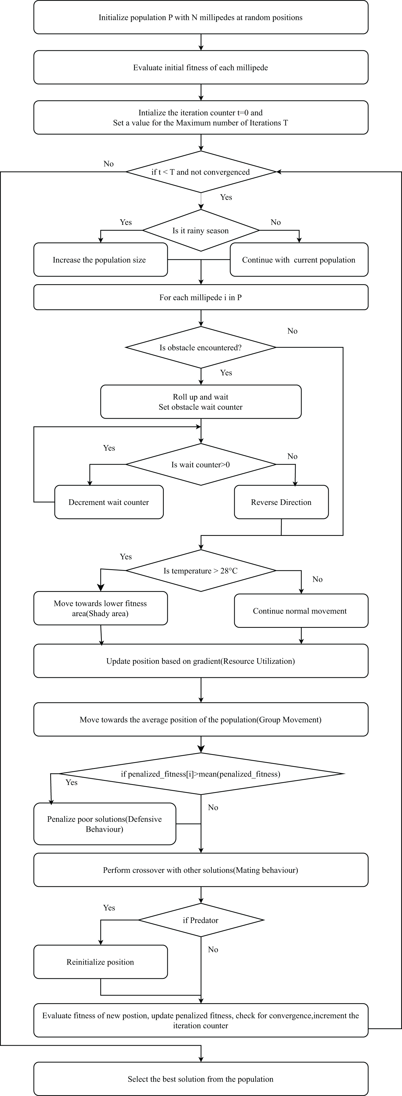
Select the best solution from the population based on the highest fitness value. Figure 4 presents the flowchart of IMOA, highlighting the initialization, fitness evaluation using mutual information, and iterative updates through seasonal activity, resource utilization, and predator avoidance. Each block corresponds to steps in Algorithm 1.
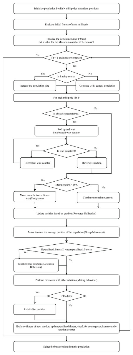
Figure 4: Flowchart of the IMOA.
Theoretical analysis of IMOA
Convergence behavior of IMOA
Optimization algorithms require a balance between global search and local refinement to ensure convergence to an optimal solution (Jia et al., 2023). IMOA achieves this by dynamically adjusting its movement strategies inspired by Indian millipede behaviors (Usha, Vasanthi & Esaivani, 2022; Dave & Sindhav, 2025; Aswathy & Sudhikumar, 2022; Ramanathan et al., 2023; Anilkumar, Wesener & Moritz, 2022). The iterative update mechanism follows a diminishing learning rate strategy, preventing stagnation in local optima while ensuring gradual convergence. A convergence proof in heuristic optimization typically relies on demonstrating that the search space coverage diminishes over time, leading the algorithm toward a stable solution (Jia et al., 2023).
Theoretical convergence guarantees
The convergence of IMOA can be analyzed through its adaptive phase transitions. In the exploration phase, the seasonal abundance (Ramanathan et al., 2023) and group movement (Usha, Vasanthi & Esaivani, 2022) behaviors allow millipedes to spread widely across the search space, reducing the likelihood of premature convergence. In the exploitation phase, temperature response (Aswathy & Sudhikumar, 2022) and resource utilization (Anilkumar, Wesener & Moritz, 2022) encourage millipedes to refine their search around promising regions, gradually stabilizing towards optimal solutions. Given that IMOA follows a structured adaptation of movement and interaction rules, it aligns with convergence properties observed in traditional nature-inspired algorithms such as GA (Fang et al., 2024), PSO (Jain et al., 2022), and GWO (Mirjalili, Mirjalili & Lewis, 2014), as shown in Table 2.
| Algorithm | Exploration strategy | Exploitation strategy | Local optima escape mechanisms | Adaptability |
|---|---|---|---|---|
| GA (Fang et al., 2024) | Random mutation | Selection pressure on fittest solution | Mutation | moderate (Static Mutation and crossover rates) |
| PSO (Jain et al., 2022) | Inertia weighted velocity updates | Position refinement based on global/local bests | No explicit escape mechanism | Moderate (Fixed inertia weight) |
| GWO (Mirjalili, Mirjalili & Lewis, 2014) | Alpha, beta, delta wolf-based exploration | Hunting mechanism via encircling prey | Leader-centric approach | Moderate (Depends on hierarchy) |
| IMOA (Proposed) | Seasonal abundance and group movement | Temperature response and resource utilization | Obstacle avoidance and Predator avoidance | High (Adaptive transition based on the optimization phase) |
Empirical evidence of convergence
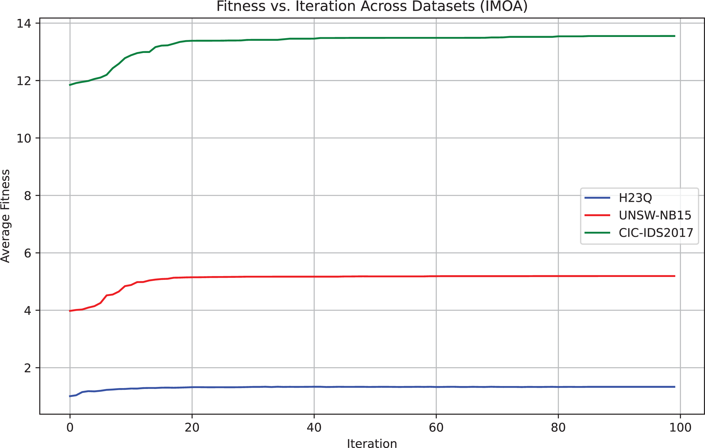
To empirically validate IMOA’s convergence, we analyze its fitness function evolution across 100 iterations on the UNSW-NB15, H23Q, and CIC-IDS2017 datasets. Figure 5 demonstrates the empirical evidence of convergence for the proposed IMOA across three benchmark datasets. The fitness curves show a consistent and smooth convergence pattern, where the algorithm rapidly improves its performance in the early iterations and gradually stabilizes as it approaches the optimal solution. CIC-IDS2017 exhibits the highest average fitness, indicating a more complex optimization landscape, while H23Q converges faster due to its relatively more straightforward structure.
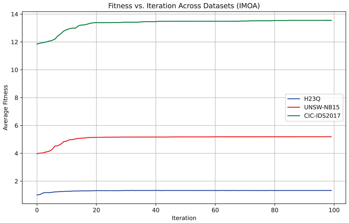
Figure 5: Convergence behavior of the IMOA across UNSW-NB15,CIC-IDS2017 and H23Q datasets.
While a universal formal proof of convergence remains a research challenge for metaheuristics, IMOA’s adaptive control mechanisms ensure stable behavior comparable to GA (Fang et al., 2024), PSO (Jain et al., 2022), and GWO (Mirjalili, Mirjalili & Lewis, 2014).
Computational complexity analysis
Theoretical complexity
The computational complexity of IMOA can be analyzed and compared with traditional metaheuristics like GA, PSO, and GWO through the key steps, namely initialization, fitness evaluation, and iterative movement. These steps define its computational complexity as shown in Table 3.
| Operation | GA (Fang et al., 2024) complexity | PSO (Jain et al., 2022) complexity | GWO (Mirjalili, Mirjalili & Lewis, 2014) complexity | IMOA complexity |
|---|---|---|---|---|
| Initialization | O (N × d) | O (N × d) | O (N × d) | O (N × d) |
| Fitness evaluation | O (N) | O (N) | O (N) | O (N) |
| Iterative update | O (N) | O (N × d) | O (N2 × d) | O (N2 × d) |
| Overall complexity | O (N × d × T) | O (N × d × T) | O (N2 × d × T) | O (N2 × d × T) |
Let N be the population size.
d be the number of features and
T be the number of iterations.
The worst-case time complexity of IMOA is
O (N2 × d × T).
In theory, from Table 3, we deduce that among the algorithms compared, IMOA and GWO (Mirjalili, Mirjalili & Lewis, 2014) have higher per-iteration costs due to their group-interaction-based update strategies, unlike GA (Fang et al., 2024) and PSO (Jain et al., 2022), which primarily rely on individual-based updates.
Runtime and fitness comparisons
To empirically validate IMOA’s computational efficiency, we conducted runtime comparisons as shown in Table 4. The runtime and fitness performance analysis compares IMOA with PSO, GWO, and GA across the UNSW-NB15, CIC-IDS2017, and H23Q datasets. IMOA demonstrates a strong balance between optimization accuracy and computational efficiency, achieving significantly lower average iteration times than PSO and GA while maintaining competitive fitness values. For instance, on the UNSW-NB15 dataset, IMOA required only 31.03 s per iteration compared to 718.38 s for PSO and 824.08 s for GA. Although GWO had the fastest runtime, its fitness performance was consistently the lowest across all datasets. These results highlight IMOA’s suitability for real-time intrusion detection applications where both speed and accuracy are essential.
| Algorithm | (UNSW-NB15) | (CIC-IDS2017) | (H23Q) | |||
|---|---|---|---|---|---|---|
| Average time per iteration in sec | Average best fitness | Average time per iteration in sec | Average best fitness | Average time per iteration in sec | Average best fitness | |
| PSO (Jain et al., 2022) | 718.3821 ± 121.7650 s | 5.4856 ± 0.3687 | 34,336.9969 ± 1,560.9912 s | 14.3848 ± 0.6970 | 1,188.7140 ± 183.7473 s | 1.4882 ± 0.0851 |
| GWO (Mirjalili, Mirjalili & Lewis, 2014) | 19.9321 ± 2.7349 s | 0.3286 ± 0.0469 | 838.9168 ± 36.9396 s | 0.5139 ± 0.0148 | 71.2276 ± 4.3994 s | 0.2478 ± 0.0786 |
| GA (Fang et al., 2024) | 824.0888 ± 141.8974 s | 5.6282 ± 0.0439 | 75,434.3345 ± 749.7889 s | 13.4396 ± 1.0739 | 1,496.4866 ± 45.3354 s | 1.6351 ± 0.0232 |
| IMOA (Proposed) | 31.0347 ± 5.0961 s | 5.0811 ± 0.3663 | 2,819.3449 ± 575.5523 s | 13.3224 ± 0.6850 | 137.0148 ± 21.3123 s | 1.3121 ± 0.0168 |
Comparative advantages of IMOA over traditional metaheuristics
While numerous nature-inspired metaheuristics such as GA (Fang et al., 2024), PSO (Jain et al., 2022), and GWO (Mirjalili, Mirjalili & Lewis, 2014) exist, they often suffer from premature convergence, limited diversity, or rigid parameter adaptation. But the IMOA is not only biologically novel but also provides algorithmic benefits due to its multi-phase behavioral modelling, as given below.
-
The seasonal abundance and group movement behaviors in IMOA allow dynamic adjustment of the exploration rate based on the optimization stage. This offers greater flexibility and adaptability compared to the static inertia weights in PSO (Jain et al., 2022) or fixed crossover and mutation rates in GA (Fang et al., 2024).
-
In IMOA, the obstacle avoidance behavior introduces directional reversal and temporary stagnation, simulating a biologically inspired pause-and-redirect mechanism. This enables the algorithm to escape local optima without relying solely on random mutation or high stochasticity. In contrast, optimizers like PSO (Jain et al., 2022) and GWO (Mirjalili, Mirjalili & Lewis, 2014) may experience premature convergence due to their fixed update equations and leader-centric designs. While standard GA (Fang et al., 2024) introduces diversity through mutation, it still requires careful tuning of mutation rates and selection pressure to avoid getting trapped in suboptimal regions.
-
Temperature response in IMOA modulates search intensity based on convergence status, while predator avoidance enables selective reinitialization of stagnated agents. These behaviors help maintain population diversity. In comparison, PSO (Jain et al., 2022) and GWO (Mirjalili, Mirjalili & Lewis, 2014) lack explicit mechanisms for diversity control or stagnation recovery, and GA (Fang et al., 2024) relies on fixed mutation rates that may be suboptimal in complex search spaces. IMOA offers a more adaptive and context-aware approach to managing exploration during optimization.
-
In IMOA, resource utilization and mating behaviors guide the search toward high-fitness regions, similar to elitism in GA (Fang et al., 2024) but driven by biologically inspired selection pressures. Unlike PSO (Jain et al., 2022), which updates positions based on global and personal bests without direct exploitation of elite zones, or GWO (Mirjalili, Mirjalili & Lewis, 2014), which relies on leader-driven convergence, IMOA enables a more focused yet diverse local search guided by adaptive biological mechanisms.
Relevance to our IDS
In the proposed WGAN-GP_IMOA_DA_Ensemble framework, the IMOA was utilized to tackle the issue of feature redundancy and high dimensionality. For example, the UNSW-NB15 dataset includes 44 features, many of which are either irrelevant or overlapping. By applying IMOA, the feature space was reduced to 22 attributes, effectively removing nearly half of the redundant features while keeping the most informative ones. This reduction directly benefits real-time IDS deployment, where faster processing allows for timely attack detection. The comparative runtime and fitness analysis shown in Table 4 illustrates IMOA’s strong balance between computational efficiency and optimization accuracy. Furthermore, the adaptive exploration–exploitation strategies embedded in IMOA, such as obstacle avoidance and resource utilization, ensure that feature selection remains both accurate and robust. This makes it more suitable for IDS environments than traditional metaheuristics like PSO, GA, or GWO.
Generative adversarial networks (GAN)
A generative model is a type of machine learning model that learns to generate new data instances that resemble the training data. Among the various generative models, the GAN (Jamoos et al., 2023) is gaining momentum due to its ability to produce highly realistic and quality data samples. The architecture of a GAN is shown in Fig. 6. The generator G creates synthetic traffic samples, while the discriminator D distinguishes between real and generated data, forming the basis of our enhanced WGAN-GP. GANs are composed of two neural networks (Cai et al., 2023): a generator and a discriminator. These networks are trained together in an adversarial process. The generator aims to create realistic data samples, while the discriminator’s objective is to differentiate between genuine and generated samples (Alsirhani et al., 2023).
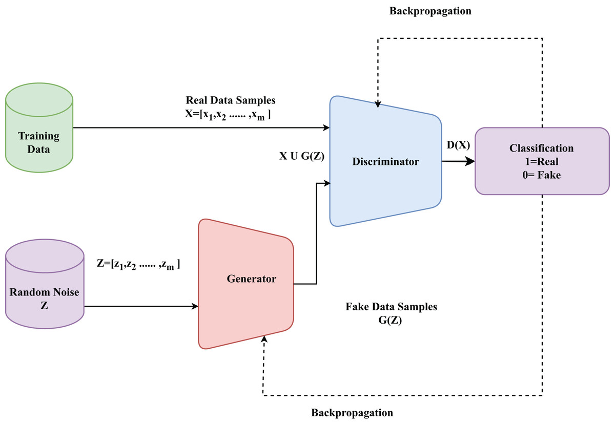
Figure 6: Basic architecture of a GAN model.
The generator G is a neural network that takes a random noise vector Z = [z1, z2,……, zm] as input and generates a fake data sample G(Z) (Jamoos et al., 2023). The discriminator D is a neural network designed to evaluate data samples and produce a probability D(x) that reflects whether the sample is authentic (originating from the real dataset) or synthetic (created by the generator) (Srivastava, Sinha & Kumar, 2023). The objective function of the GANs is a minimax game between the generator and the discriminator. The generator tries to minimize the objective while the discriminator tries to maximize it. The objective function of G can be formulated as shown in Eq. (16) (Srivastava, Sinha & Kumar, 2023).
(16)
The objective function of D can be formulated as shown in Eq. (16) (Srivastava, Sinha & Kumar, 2023).
(17)
Clearly, GAN can be formulated as a minmax problem where is a value function and is defined in Eq. (18).
(18) where is a real data sample from the true data distribution .
is a random noise vector sampled from a prior distribution
is the generated data sample from the generator.
is the probability that is a real data sample.
is the probability that the generated sample It is a real data sample.
Some of the most widely used GAN models are Vanilla GAN (Jamoos et al., 2023), Conditional GAN (cGAN) (Devendiran & Turukmane, 2024), Deep Convolutional GAN (DCGAN) (Cai et al., 2023) and WGAN (Park et al., 2022). Among these models, WGAN uses the Wasserstein distance that encourages the generation of diverse samples and yields better-quality generated samples. WGAN-GP is a variation of WGAN in which the Wasserstein distance with gradient penalty is used to improve the training stability and alleviate issues such as mode collapse (Alsirhani et al., 2023). This research utilized WGAN-GP to tackle the problem of an imbalanced dataset by generating synthetic data samples that are similar to the original data samples. The WGAN utilizes the Wasserstein distance to measure the difference between the real and generated data distributions. The Wasserstein distance between two probability distributions and is given by Eq. (19) (Alsirhani et al., 2023).
(19) where denotes the set of all joint distributions γ( ) whose margins are respectively. γ( ) denotes the expectation is taken over pairs ( ) sampled from the joint distribution γ.
In WGAN-GP, the critic (discriminator) D is trained to approximate the Wasserstein distance, while the generator G is trained to minimize it. The objective function of the critic is given in Eq. (20) (Alsirhani et al., 2023).
(20) where is the gradient penalty coefficient is generated data and are the samples interpolated between real and generated data.
To ensure the critic is a 1-Lipschitz function (required for Wasserstein distance), WGAN-GP uses a gradient penalty instead of weight clipping. The gradient penalty is calculated as
(21)
With the ability to provide high-quality and diverse synthetic samples that improve model robustness and detection accuracy, WGAN-GP shows potential in augmenting data for IDS (Alsirhani et al., 2023). By using the Wasserstein distance and gradient penalty, WGAN-GP produces realistic data that accurately replicates the intricate patterns of network traffic and ensures stable training (Alsirhani et al., 2023). This improves the ability of the IDS to identify new and sophisticated attacks that may not be well represented in the original dataset. The practical training process of our enhanced WGAN-GP, which incorporates attention layers, normalization, and skip connections in the discriminator, is summarized in Algorithm 2.
| Input: Real training data Xreal, Noise distribution Z, Number of training steps T |
| Parameters: λ (gradient penalty coefficient), learning rates αG and αD |
| Output: Trained Generator G and Discriminator D |
| 1. Initialize Generator G and Discriminator D with random weights. |
| • Add attention layers, layer normalization, and skip connections to D for stability. |
| 2. For each training iteration t = 1 to T: |
| 2.1 Sample real data batch x from minority classes (e.g., Worms, Heartbleed). |
| 2.2 Sample noise vector z from distribution Z (e.g., Gaussian). |
| 2.3 Generate synthetic samples: |
| - = G(z) |
| 2.4 Update Discriminator D: |
| • Compute real score: Dr = D(x) |
| • Compute fake score: Df = D( ) |
| • Compute gradient penalty (Eq. (21)): |
| • Update D by minimizing loss: |
| LD = Df − Dr + GP |
| 2.5 Update Generator G: |
| • Sample noise vector z → generate . |
| • Update G by minimizing: |
| LG = −D( ) |
| 3. Repeat steps 2.1–2.5 until convergence. |
| 4. Return trained G and D. |
| • Use G to augment minority classes in the IDS dataset, balancing the distribution. |
WGAN-GP—relevance to our IDS
The application of enhanced WGAN-GP effectively addresses the severe class imbalance issue in IDS datasets. As shown in Table 5, minority classes such as Infiltration with 36 samples, Heartbleed with 11 samples, and Worms with 174 samples were augmented to several thousand synthetic samples. As a result, imbalance ratios are reduced from extreme values like 1:50 to near-balanced distributions such as 1:3. This augmentation is significant because conventional classifiers tend to bias toward majority classes, leading to poor recall on rare but high-impact attacks.
| Dataset | Minority classes | Number of Instances | Generated synthetic data instances using WGAN-GP | Total number of instances |
|---|---|---|---|---|
| CIC-IDS2017 | Infiltration | 36 | 4,327 | 4,363 |
| Web Attack-Sql Injection | 21 | 2,586 | 2,602 | |
| Heartbleed | 11 | 1,791 | 1,802 | |
| H23Q | Quic-enc | 1,663 | 2,000 | 3,663 |
| http-smuggle | 508 | 2,000 | 2,508 | |
| UNSW-NB15 | Worms | 174 | 2,784 | 2,958 |
By generating realistic synthetic traffic patterns, WGAN-GP improves both the diversity and representativeness of training data. For instance, the UNSW-NB15 Worms class expanded from 174 to 2,958 instances, while CIC-IDS2017 Heartbleed increased from 11 to 1,802 instances. These enriched datasets enhance the learning capability of the ensemble classifier, enabling more reliable detection of rare intrusions.
Overall, the integration of WGAN-GP into our IDS pipeline transforms theoretical generative modeling into a practical solution for skewed data distributions. It leads to measurable improvements in performance for minority attacks without introducing significant overfitting.
Proposed methodology
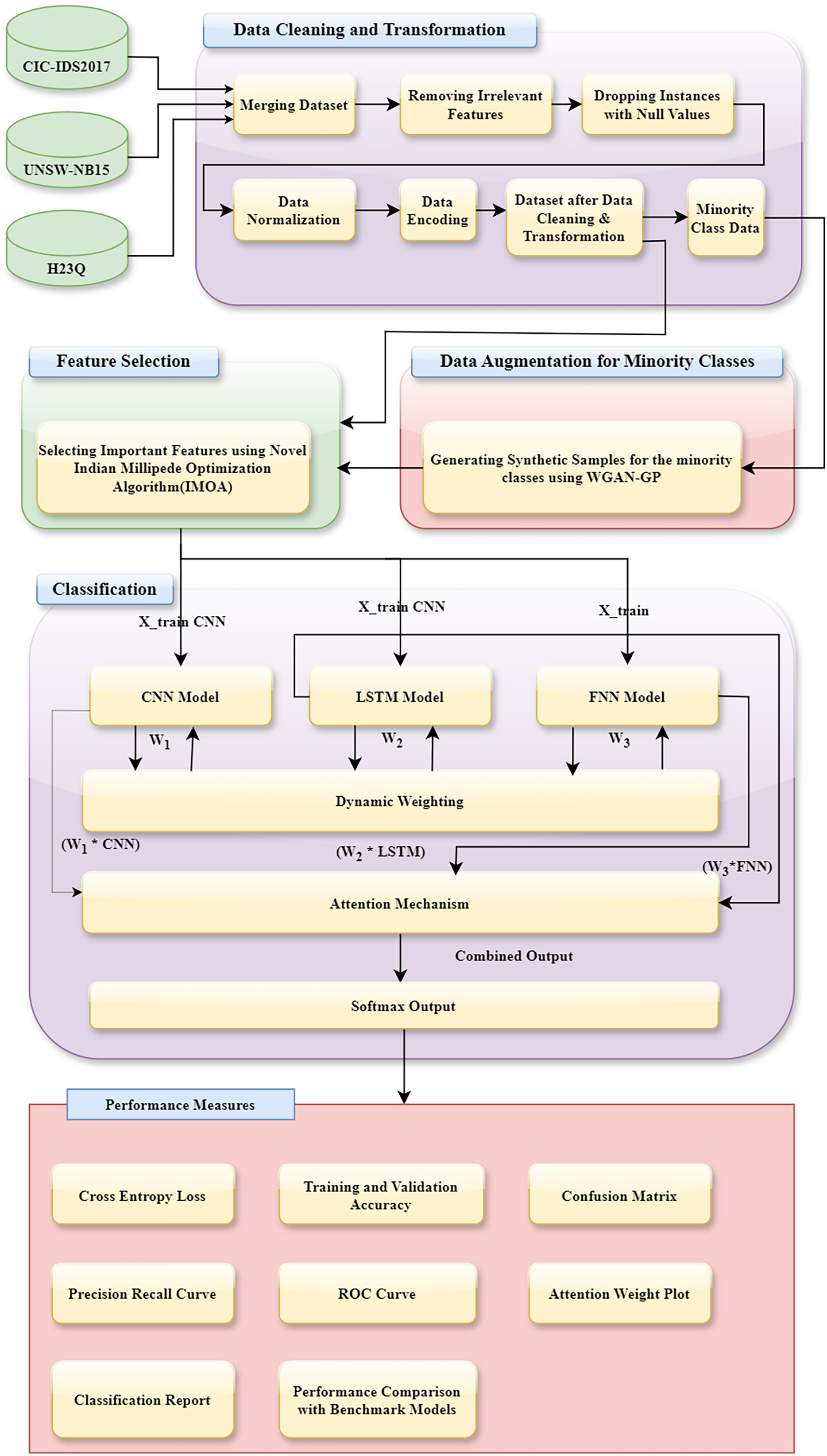
This section provides the details of the proposed methodology. It has five significant steps. (1) Description of datasets used, (2) initial data preprocessing, (3) data augmentation with WGAN-GP, (4) feature selection using IMOA, and (5) classification using a DA_Ensemble approach. The complete workflow of our IDS is illustrated in Fig. 7. The pipeline integrates IMOA-based feature selection, WGAN-GP augmentation for class balancing, and a DA based ensemble classifier for final decision-making.
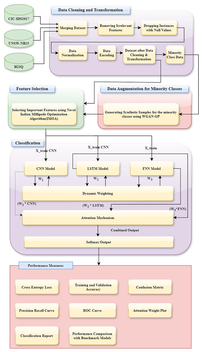
Figure 7: Architecture of the proposed WGAN-GP_IMOA_DA_Ensemble method for intrusion detection.
Dataset description
This section gives a detailed description of the datasets used in this research. It uses three datasets, namely (i) CIC-IDS2017, (ii) UNSW-NB15, and (iii) H23Q, to evaluate the effectiveness of the suggested IDS as described by Table 6.
| Dataset | Attacks | Number of instances | Total .CSV files | Instances used in experiment | Number of features |
|---|---|---|---|---|---|
| CIC-IDS2017 | 1. BENIGN | 2,273,097 | Eight files in total | 2,273,097 | 79 |
| 2. DoS Hulk | 231,073 | 231,073 | |||
| 3. PortScan | 158,930 | 158,930 | |||
| 4. DDoS | 128,027 | 128,027 | |||
| 5. DoS GoldenEye | 10,293 | 10,293 | |||
| 6. FTP-Patator | 7,938 | 7,938 | |||
| 7. SSH-Patator | 5,897 | 5,897 | |||
| 8. DoS slowloris | 5,796 | 5,796 | |||
| 9. DoS Slowhttptest | 5,499 | 5,499 | |||
| 10. Bot | 1,966 | 1,966 | |||
| 11. Web Attack Brute Force | 1,507 | 1,507 | |||
| 12. Web Attack XSS | 652 | 652 | |||
| 13. Infiltration | 36 | 36 | |||
| 14. Web Attack Sql Injection | 21 | 21 | |||
| 15. Heartbleed | 11 | 11 | |||
| Total | 2,830,743 | 2,830,743 | |||
| UNSW-NB15 | 1. Normal | 93,000 | Two files (Train file, test file) | 93,000 | 45 |
| 2. Generic | 58,871 | 58,871 | |||
| 3. Exploits | 44,525 | 44,525 | |||
| 4. Fuzzers | 24,246 | 24,246 | |||
| 5. DoS | 16,353 | 16,353 | |||
| 6. Reconnaissance | 13,987 | 13,987 | |||
| 7. Analysis | 2,677 | 2,677 | |||
| 8. Backdoor | 2,329 | 2,329 | |||
| 9. Shellcode | 1,511 | 1,511 | |||
| 10. Worms | 174 | 174 | |||
| Total | 257,673 | 257,673 | |||
| H23Q | 1. Normal | 95,69,662 | In all 60 files | 1,372,539 | 200 |
| 2. HTTP3-flood | 498,810 | 6 | 62,383 | ||
| 3. Fuzzing | 22,224 | 6 | 8,046 | ||
| 4. HTTP3-loris | 74,572 | 6 | 17,502 | ||
| 5. QUIC-flood | 61,340 | 6 | 17,159 | ||
| 6. QUIC-loris | 24,269 | 6 | 3,762 | ||
| 7. QUIC-enc | 5,829 | 6 | 1,663 | ||
| 8. HTTP-smuggle | 3,337 | 6 | 508 | ||
| 9. HTTP2-concurrent | 60,273 | 6 | 8,980 | ||
| 10. HTTP2-pause | 53,549 | 6 | 7,458 | ||
| Total | 10,401,928 | 60 files | 1,500,000 |
UNSW-NB15
The UNSW-NB15 dataset is a comprehensive intrusion detection dataset created by the Australian Centre for Cyber Security (ACCS) (Otair et al., 2022). It is freely available for download at https://research.unsw.edu.au/projects/unsw-nb15-dataset. It consists of two .csv files, namely “UNSW_NB15_training_set.csv” of 175,341 instances and “UNSW_NB15_testing_set.csv” of 82,332 instances. It contains a total of 257,673 instances. It has nine attack categories. Various attacks and their total number of occurrences in the dataset are depicted in Table 6. It has 45 features, including four categorical features and 41 numerical features. The t-distributed Stochastic Neighbor Embedding (t-SNE) visualizations of binary and multiclass labels for this dataset are shown in Figs. 8A and 8D, respectively.
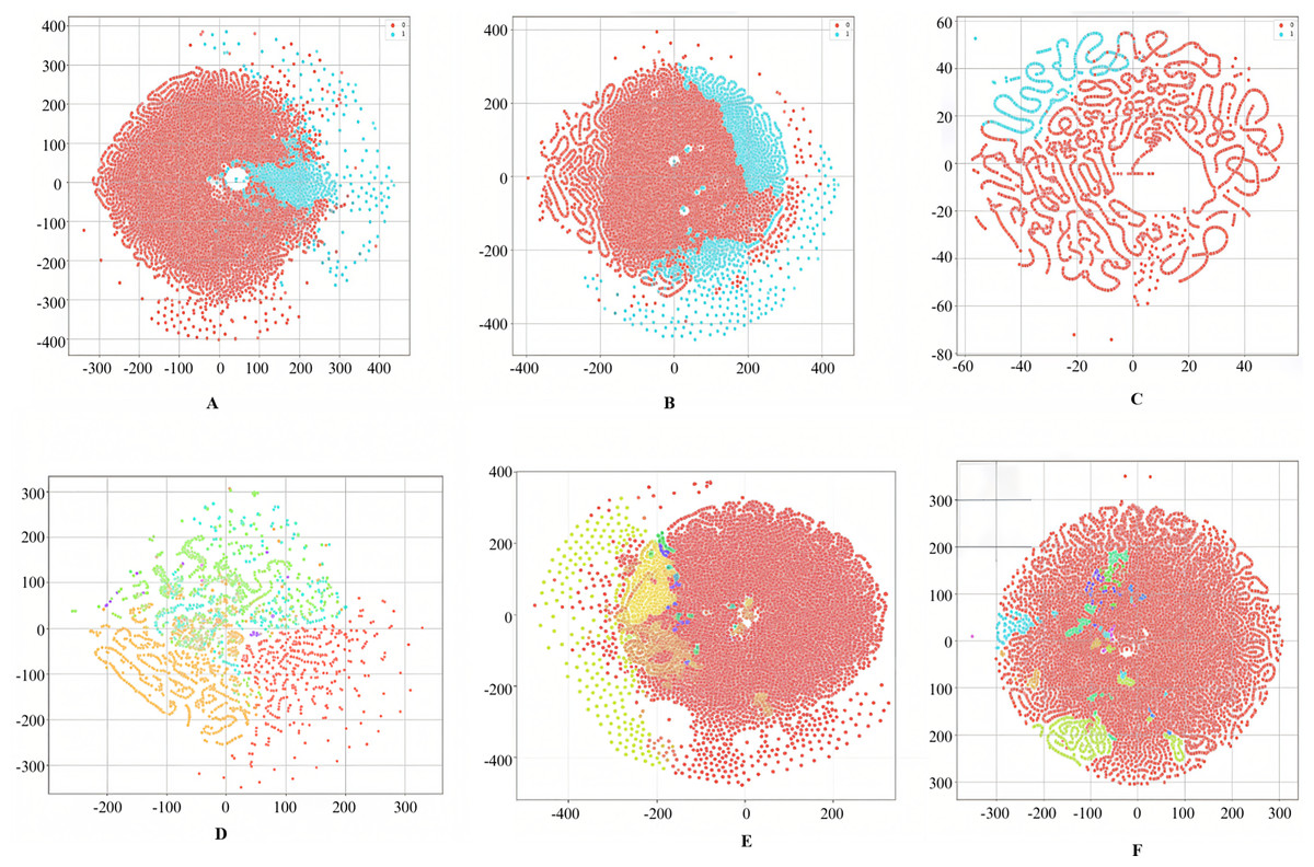
Figure 8: t-SNE visualizations of the WGAN-GP_IMOA_DA-Ensemble model for binary (A–C) and multiclass (D–F) classification on UNSW-NB15, CIC-IDS2017, and H23Q datasets.
t-SNE plots illustrating the feature space separation achieved by the proposed model for both binary and multi-class classification tasks across the UNSW-NB15, CIC-IDS2017, and H23Q datasets. Each color represents a distinct class label.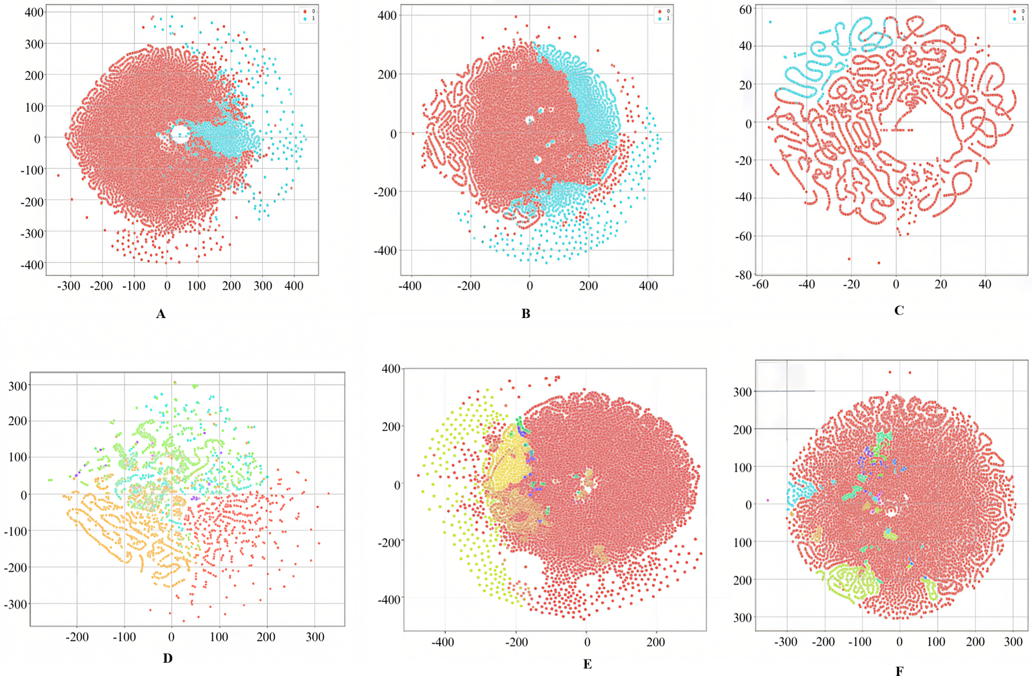
CIC-IDS 2017
The Canadian Institute for Cybersecurity IDS (CIC-IDS) 2017 dataset is a comprehensive dataset designed for evaluating the performance of IDS (Jia et al., 2023). It is freely available for download at https://www.unb.ca/cic/datasets/ids-2017.html. It has 2,273,097 instances of benign samples. In addition, it has 14 attack types of a total of 557,646 instances, as shown in Table 6. It has 79 features. It has all numeric features except the label. The t-SNE visualizations of binary and multiclass labels for this dataset are shown in Figs. 8B and 8E, respectively.
H23Q
The H23Q Dataset is a comprehensive 802.3 dataset containing labelled (Aljehane et al., 2024) traces of ten attack types against Hypertext Transfer Protocol (HTTP)/2, HTTP/3, and Quick UDP (User Datagram Protocol) Internet Connections (QUIC) services, with a focus on modern HTTP/3-specific attacks. Available at https://icsdweb.aegean.gr/awid/other-datasets/H23Q in pcap and CSV formats, it has 9,569,662 normal instances and 804,203 attack instances. Additionally, this dataset has 200 features, as shown in Table 6. It has all numeric features except the label. The t-SNE visualizations of binary and multiclass labels for this dataset are shown in Figs. 8C and 8F, respectively.
Initial data preprocessing
Data preprocessing, also known as data preparation, is the process of transforming raw data into a clean and usable format (Fraihat et al., 2023). The main aim of data preprocessing is to improve the quality of the data. The proposed model uses the following data preprocessing techniques.
Merging datasets (data integration)
Usually, the IDS dataset is very large in size and is available in chunks of many files. To make use of the complete dataset for the comprehensive analysis or modelling, all the chunks need to be merged (Moustafa & Slay, 2015). Table 6 provides the count of files in each dataset, along with the total number of features and instances for each one (Fraihat et al., 2023). The CIC-IDS2017 dataset consists of a total of eight .csv files, while the UNSW-NB15 dataset contains two files. In contrast, the H23Q dataset comprises sixty files. For the CIC-IDS2017 and UNSW-NB15 datasets, all the files have been merged for utilization. Due to the substantial size of the H23Q dataset, which is 30 GB, a sample of 150,000 instances for each attack type has been extracted, resulting in a total of 1,500,000 instances for experimentation.
Data cleaning
Data cleaning is the process of identifying and correcting or removing errors or inconsistencies in the dataset (Hanafi et al., 2023). The data cleaning techniques employed for the CIC-IDS2017 dataset include removing columns that are entirely homogeneous and dropping rows with NA values. For the UNSW-NB15 dataset, the methods applied involve eliminating the ‘id’ column, which is deemed unnecessary; checking for any missing values and removing those rows; and replacing categorical columns with a value of ‘-’ with ‘None.’ In the case of the H23Q dataset, missing values for categorical features are filled using mode imputation, while numerical features are addressed with mean imputation.
Data Transformation
Data encoding is a kind of data transformation where categorical data are converted into numerical data as required by modelling and analysis (Bowen et al., 2023). In this study, label encoding was utilized for all the categorical features in binary classification to reduce dimensionality. Conversely, one-hot encoding was employed for the ‘Label’ feature in multiclass classification to avoid making any ordinal assumptions among the multiple classes. Data normalization is a data transformation technique where numerical data is scaled to a consistent range, such as 0–1 (Fraihat et al., 2023).
Min-Max Scaling: Min-max scaling transforms features to a fixed range, usually 0 and 1 (Hanafi et al., 2023). The formula for min-max scaling is
(22)
Min-max scaling was applied to the CIC-IDS 2017 and UNSW-NB15 datasets to normalize features within a bounded range of [0, 1], because these datasets have limited outlier influence.
Z-Score Scaling: Z-score scaling, also known as standardization, transforms the data to have a mean of 0 and a standard deviation of 1 (Sajid et al., 2024). The formula for z-score scaling is:
(23)
Standard scaling (z-score scaling) was utilized for the H23Q dataset, given its larger size and potentially diverse feature distributions, ensuring that all features had a mean of 0 and a standard deviation of 1 while being less sensitive to outliers.
Data augmentation with WGAN-GP
This research utilizes the WGAN-GP model to generate synthetic samples for the minority classes to address the class imbalance problem. The details of various parameters of WGAN-GP used in this study are given in Table 7. This noise vector, z ~ N(0, 1), has a dimension of z_dim = 10. The generator network has three fully connected layers, each followed by batch normalization and a Leaky ReLU activation function. The generator’s output layer applies a tanh activation function. The discriminator D is also composed of three dense layers, each followed by Leaky ReLU activations. Its final layer outputs a single scalar value D(x) for a given input x. After training, the generator G is used to produce synthetic data samples corresponding to the minority classes identified in CIC-IDS2017, UNSW-NB15, and H23Q, as shown in Table 5. For example, in UNSW-NB15, the discriminator assigns higher scores to synthetic ‘Worms’ traffic that resembles real samples, penalizing only when gradients deviate significantly from 1. This stabilizes training and avoids mode collapse. Specifically, for CIC-IDS2017, synthetic data is generated for the classes Infiltration, Web Attack—SQL Injection, and Heartbleed. In contrast, for UNSW-NB15, the targeted class is Worms, and for H23Q, they are quic-enc and http-smuggle. The created augmented dataset combines both real and synthetic samples, denoted by Xcombined and ycombined. This augmented dataset is subsequently used to train the final detection model.
| Variable | Value |
|---|---|
| z_dim | 10 |
| gp_weight | 10.0 |
| batch_size | 128 |
| epochs | 50 |
| input_dim | Based on X |
| output_dim | Based on X |
| generator_optimizer | Adam (learning rate: 10−4) |
| discriminator_optimizer | Adam (learning rate: 10−4) |
| real_data | Based on X |
| noise | Sampled from a normal distribution with dimension z_dim |
IMOA-based feature selection
Feature selection is a data pre-processing method that reduces the number of features of a dataset that is fed as input to an artificial intelligence model. It enhances the performance of the learning models by keeping only the most significant features (Moustafa & Slay, 2015). Various techniques, such as wrapper methods, filter methods, and embedded methods, are available for feature selection (Chatzoglou et al., 2023). Recently, researchers have shown phenomenal interest in using optimization algorithms for feature selection due to the improved model performance (Bowen et al., 2023). This article utilizes the IMOA algorithm for feature selection from the datasets.
IMOA mechanisms in feature selection
In this application, IMOA’s objective is to maximize the relevance of selected features based on their mutual information with the target variable (attack type or benign). This is formulated as a fitness function given in Eq. (24).
(24) where f is a binary mask indicating selected features, Xj denotes a specific feature in the dataset, and y represents the target class labels. For instance, in UNSW-NB15, IMOA evaluates feature sbytes by calculating its mutual information with the attack label. A higher MI score indicates that this feature strongly correlates with attack presence, hence it is more likely to be selected. The mutual information, MI (Xj, y), measures the statistical dependency between each selected feature Xj and y, guiding the algorithm towards high-information features. The parameter configuration of IMOA for feature selection is given in Table 8.
| Parameter | Value |
|---|---|
| Population size (N) | 20 |
| Dimensions (d) | Feature count varies based on the dataset |
| Maximum iterations (T) | 100 |
| Seasonal activity (α) | 0.1 |
| Reversal factor (β) | 0.5 |
| Learning rate (γ) | 0.1 |
| Penalty coefficient (λ) | 10 |
| Crossover coefficient (η) | 0.5 |
| Batch size | 128 |
| No improvement limit | 10 |
For each mask, the fitness function evaluates the relevance of the selected features based on mutual information. Penalized fitness is calculated by subtracting the product of the penalty coefficient = 10 and any constraint violation. In this application, there are no hard constraints, so constraint violations are zero, simplifying the penalized fitness to the raw fitness score. Through iterative updates and fitness evaluations, IMOA identifies the optimal subset of features for each dataset.
Outcome and final feature set
The IMOA was applied to CIC-IDS2017, UNSW-NB15, and H23Q to select the most informative features based on mutual information with respect to attack labels. The selected features help in distinguishing between normal and malicious network traffic while maintaining the balance between detection accuracy and computational efficiency. This optimized feature subset reduces computational overhead, allowing the IDS to operate efficiently even in real-time environments. The resulting feature sets are given in Table 9.
| Dataset | Selected features count | Selected features |
|---|---|---|
| CIC-IDS2017 | 40 | Total Backward Packets, Total Length of Fwd Packets, Total Length of Bwd Packets, Fwd Packet Length Max, Fwd Packet Length Min, Fwd Packet Length Std, Bwd Packet Length Min, Bwd Packet Length Std, Flow IAT Std, Flow IAT Max, Flow IAT Min, Fwd IAT Max, Fwd IAT Min, Bwd IAT Mean, Bwd IAT Max, Bwd IAT Min, Fwd URG Flags, Fwd Header Length, Bwd Header Length, Bwd Packets/s, Max Packet Length, Packet Length Mean, Packet Length Variance, SYN Flag Count, RST Flag Count, PSH Flag Count, ACK Flag Count, URG Flag Count, CWE Flag Count, Down/Up Ratio, Average Packet Size, Avg Fwd Segment Size, Avg Bwd Segment Size, Subflow Fwd Packets, Subflow Bwd Packets, Subflow Bwd Bytes, Active Mean, Active Max, Active Min, Idle Std |
| H23Q | 14 | Frame. Time, frame.time_epoch, frame.time_delta, frame.time_delta_displayed, frame.time_relative, frame.len, ip.hdr_len, ip.dsfield.dscp, ip.dsfield.ecn, ip.flags.df, ip.flags.mf, ip.ttl, ip.src, ip.dst |
| UNSW-NB15 | 22 | dur, proto, service, state, sbytes, dbytes, dload, sloss, sinpkt, sjit, swin, stcpb, dtcpb, dwin, synack, ackdat, dmean, trans_depth, ct_state_ttl, ct_dst_src_ltm, ct_ftp_cmd, ct_src_ltm |
Dynamic attention-based ensemble mechanism for intrusion detection
This research proposes a DA_Ensemble ensemble mechanism for classification that combines predictions from three distinct models: a CNN, LSTM, FNN to enhance the classification accuracy. This ensemble method utilizes the individual strengths of each model and dynamically assigns weights based on their validation accuracy, allowing the ensemble to focus on the models with the highest predictive performance. This section provides an overview of each model, describing the model architecture along with the parameters applied in this research and an explanation of the dynamic attention mechanism.
Convolutional Neural Network (CNN)
A CNN is a deep learning method that learns and identifies patterns from raw data by using filters (or kernels) that slide across the input data and capture local features (Kareem et al., 2022). The basic architecture of a CNN consists of three main types of layers (Kareem et al., 2022):
Convolutional Layers: These layers perform convolutions, which involve applying filters to small regions of the input data. Each filter in a convolutional layer is a matrix of weights that is learned during training. For a single convolution operation, a filter W of size k × k is applied to an input X, producing an output (feature map) h, calculated as
(25) where represents the dot product between the filter and the input region, b is the bias term, and f is a non-linear activation function.
In the proposed model, the 1D convolutional layer is configured with 64 filters and a kernel size of 3, followed by the ReLU activation function.
Pooling Layers: A pooling layer downsamples a feature map from a convolutional layer by selecting the maximum value from each sub-region (Bella et al., 2024). The pooled value is given by Eq. (26).
(26) where is the pooled value, and represents the values within the pooling window. The proposed model utilizes a global average pooling layer, which reduces the dimensionality of the feature maps by taking the average value of each feature map across all positions.
Fully Connected Layers: At the end of the CNN, fully connected layers take the flattened feature maps and apply a series of dense connections to combine features across the entire input, resulting in an output suitable for classification (Kareem et al., 2022). This research employs a fully connected layer with 128 units. A sigmoid activation function in the output layer for binary classification and SoftMax activation for multiclass classification.
Long Short-Term Memory (LSTM)
LSTM networks are a special type of recurrent neural network (RNN) that excel at capturing dependencies over long sequences of data (Chinnasamy, Malliga & Sengupta, 2022). The fundamental structure of an LSTM consists of memory cells and a series of gates (Ahmed et al., 2024). The main gates in an LSTM cell.
Forget Gate: It controls whether the information from the previous cell state is retained or forgotten. This is given by Eq. (27).
(27) where is the forget gate‘s output, and are weights and biases, is the previous hidden state, and is the current input (Chinnasamy, Malliga & Sengupta, 2022). The activation function (sigmoid) scales the output between 0 and 1 (Ahmed et al., 2024).
Input Gate: It determines how much new information will enter the cell state from the current input (Chinnasamy, Malliga & Sengupta, 2022). It consists of an input update and the input gate activation is given by Eqs. (28) and (29).
(28)
(29)
Here, regulates the input’s influence on the cell state, while represents a candidate update to the cell state (Chinnasamy, Malliga & Sengupta, 2022).
Output Gate: It controls the amount of information passed to the next layer or output by adjusting the hidden state (Ahmed et al., 2024). This is given by Eq. (30).
(30) where is the output gate value. The final hidden state for the time step is calculated with the Eq. (31) (Chinnasamy, Malliga & Sengupta, 2022).
(31)
This research utilizes a single LSTM layer with 128 units, batch normalization, a dense layer with 64 units, and a ReLU activation function. This research utilizes a Sigmoid activation function in the output layer for binary classification and SoftMax activation for multiclass classification.
Feedforward Neural Networks (FNN)
FNNs consist of layers of interconnected nodes (neurons) where information moves in one direction—from the input layer, through one or more hidden layers, and finally to the output layer (Moustafa & Slay, 2015). Each neuron in an FNN performs a weighted sum of its inputs and passes this through an activation function. The operation of a single neuron is given by the Eq. (32) (Moustafa & Slay, 2015).
(32) where is the input vector, is the weight matrix associated with the connections, is the bias term, σ is the activation function, such as ReLU, sigmoid, or tanh, is the output. This research has an FNN with three fully connected layers as given below. It has an input layer that accepts a set of network traffic features, which are then passed to the subsequent hidden layers. The first hidden layer contains 128 units and uses the ReLU activation function. The second hidden layer contains 64 units, also with ReLU activation. The output layer utilizes a sigmoid activation function in the output layer for binary classification and a SoftMax activation function for multiclass classification.
Dynamic attention-based ensemble
The dynamic attention mechanism is an approach in machine learning that selectively focuses on certain parts of input data based on the relevance to a specific task, enhancing model interpretability. Unlike static attention mechanisms, where attention weights are predetermined, dynamic attention recalculates these weights in real-time, adapting to each input instance and thereby allowing the model to dynamically adjust its focus (Moustafa & Slay, 2015). The dynamic attention mechanism involves assigning a score or weight to each input feature or part of the input sequence, which determines its contribution to the final output (Sharafaldin, Lashkari & Ghorbani, 2018). Attention weights for each input is calculated with Eq. (33).
(33) where is a scoring function that evaluates the relevance of . The exponential function normalizes the scores to form a probability distribution (Sharafaldin, Lashkari & Ghorbani, 2018). The final attention-weighted output combines the inputs according to their weights, as shown in Eq. (34).
(34)
In this study, the dynamic attention mechanism specifically utilizes the outputs of the CNN, LSTM, and FNN models to adaptively weight each model’s contribution based on its relevance to the input instance. The models CNN, LSTM, and FNN produce a predictive output for a given input instance. For example, when analyzing Distributed Denial of Service (DDoS) traffic, CNN output receives the highest attention weight of around 0.6, whereas for sequential attacks such as infiltration, LSTM is prioritized. This research uses a cosine similarity function to compute the similarity between each model’s output vector and the ideal target vector y. The relevance score si for each model i is computed with Eq. (35).
(35) where is the output vector of model , is the target vector and measures the alignment between the model’s prediction and the target output. Once the relevance score for CNN, LSTM, and FNN are calculated, these scores are passed through a softmax function to transform them into attention weights . The attention weight for each model is computed with Eq. (36).
(36) where is the relevance score for model , ensures non-negativity and emphasizes higher relevance scores, the sum acts as a normalization factor across all models. The final output of the ensemble is computed as a weighted sum of the outputs from the CNN, LSTM, and FNN models. Each model’s output is scaled by its respective attention weight to form the final prediction. The final output is calculated with Eq. (37).
(37) where represents the output vector of model and is the attention weight for model i.
The dynamic fusion of CNN, LSTM, and FNN outputs using attention weights is detailed in Algorithm 3, which illustrates the complete classification process of our ensemble model.
| Input: Preprocessed feature set X |
| Base Models: Convolutional Neural Network (CNN), Long Short-Term Memory (LSTM), Feedforward Neural Network (FNN) |
| Output: Final class prediction Ypred |
| 1. Extract features from input X: |
| • Pass X through CNN to obtain local spatial feature representation HCNN. |
| • Pass X through LSTM to capture temporal dependencies HLSTM. |
| • Pass X through FNN to learn global feature interactions HFNN. |
| 2. Normalize outputs of all three models to a uniform dimensional space. |
| 3. Compute attention weights for each model: |
| • Concatenate [HCNN, HLSTM, HFNN] into a joint feature vector. |
| • Apply attention mechanism (Eqs. (32)–(34)): |
| ▪ Compute similarity scores between model outputs and target context. |
| ▪ Normalize scores via softmax to obtain attention weights: |
| wCNN, wLSTM, wFNN |
| 4. Fuse model outputs dynamically: |
| • Compute weighted sum of outputs: |
| Hfusion = wCNN HCNN + wLSTM HLSTM + wFNN HFNN. |
| 5. Feed fused representation into a final dense + softmax layer for classification. |
| 6. Return prediction Ypred for each input instance. |
Theoretical justification of the attention mechanism
The attention mechanism serves as a dynamic weighting strategy that allows the model to focus selectively on more informative components of the input or intermediate representations. Theoretically, attention can be interpreted as a form of soft feature selection, where importance scores are assigned to each input or sub-model output based on their learned relevance to the target task (Momand, Jan & Ramzan, 2024). In our ensemble model, attention weights are computed using a trainable dense layer followed by a SoftMax activation, ensuring that the weights are positive and sum to one. This formulation enables the network to adaptively emphasize the outputs of the CNN, LSTM, or FNN sub-models depending on the specific characteristics of each input instance. From an optimization perspective, this setup introduces inductive bias that can help reduce overfitting by guiding the model to rely more heavily on the most relevant components, especially in cases of class imbalance or noisy data. Although a full theoretical proof of optimality for attention mechanisms in deep ensembles is still an open problem, recent literature (Momand, Jan & Ramzan, 2024; Cai et al., 2023) supports its role in improving representational capacity and model interpretability.
DA_Ensemble—relevance to our IDS
The proposed dynamic attention-based ensemble directly enhances intrusion detection by adaptively weighting the contributions of CNN, LSTM, and FNN learners. Unlike static ensembles that assign equal or fixed weights, the attention mechanism dynamically adjusts weights according to the confidence of each model for a given traffic flow. For example, in CIC-IDS2017, CNN received higher attention scores when processing DDoS flows due to its strength in capturing local packet patterns. At the same time, LSTM was prioritized for Infiltration and Slowloris attacks, where temporal dependencies are critical.
This adaptive fusion ensures that no single learner dominates across all attack types, thereby reducing bias and improving robustness. Empirical evaluation shows that the attention-based ensemble outperforms simple majority-voting or averaging ensembles, achieving higher accuracy and lower false-positive rates, particularly on rare attack classes that benefit from the complementary strengths of different deep learning models.
By explicitly mapping theoretical attention weights to model outputs, the ensemble translates mathematical formulation into a practical mechanism for IDS, delivering a more context-aware and attack-specific detection capability.
Replication rationale and comparative validation
In addition to proposing a novel IDS framework, we designed parts of our methodology to replicate and validate existing GAN-based data augmentation and ensemble classification techniques under new conditions. Specifically,
We replicate WGAN-GP’s role in addressing class imbalance, as applied in prior works such as Park et al. 2022 and Lee, Li & Li 2023 by deploying it across three benchmark datasets: UNSW-NB15, CIC-IDS2017, and H23Q. However, we go beyond mere replication by introducing architectural improvements to the WGAN-GP discriminator, including attention layers, layer normalization, and skip connections. These enhancements enable the discriminator to better capture fine-grained patterns in minority-class data, resulting in more realistic and diverse synthetic samples, which improve downstream classification performance.
We also replicate ensemble-based IDS architectures such as CNN+LSTM and CNN+FNN as seen in works by Meliboev, Alikhanov & Kim (2022), Altunay & Albayrak (2023), and Chatzoglou et al. (2023). In our study, these are extended with a dynamic attention mechanism and informed by optimization-driven feature selection using our proposed IMOA. This integration allows for adaptive weighting of models based on relevance.
By framing these components as replications and extensions, we provide both validation of previously established techniques and a demonstration of their improved effectiveness under new conditions, including imbalanced data distributions, high-dimensional feature spaces, and a modern, large-scale dataset like H23Q. This approach strengthens the reproducibility and comparative validation of our work.
Experimental results and discussion
In this section, we present the experimental results obtained from applying our proposed WGAN-GP_IMOA_DA_Ensemble approach to three benchmark datasets. Here, we analyze the performance of the CNN, LSTM, and FNN models as an ensemble with the dynamic attention mechanism, focusing on metrics such as accuracy, precision, recall, F1-score, and loss. The downstream effects of IMOA, WGAN-GP, and dynamic attention on loss, accuracy, ROC, and PR are analyzed in Figs. 9–13, with learned attention patterns in Figs. 14, 15.
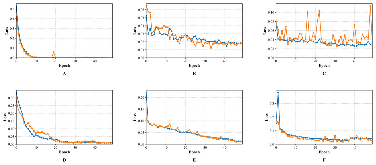
Figure 9: Training and validation loss curves of the WGAN-GP_IMOA_DA-Ensemble model for binary (A–C) and multiclass (D–F) classification on UNSW-NB15, CIC-IDS2017, and H23Q datasets.
Subplots (A–C) show binary classification loss curves, and (D–F) show multiclass classification loss curves on UNSW-NB15, CIC-IDS2017, and H23Q datasets using the proposed model.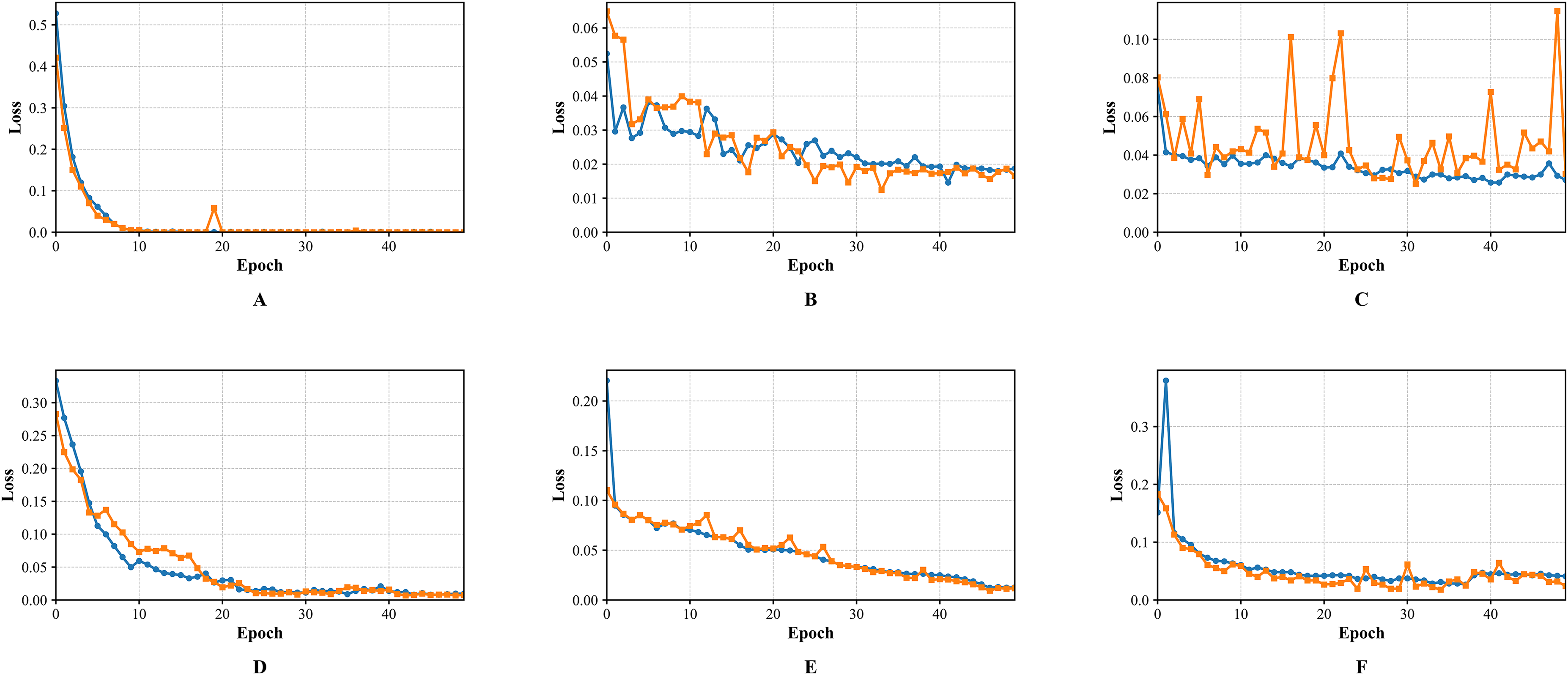
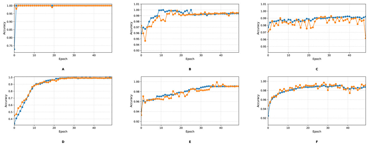
Figure 10: Training and validation accuracy curves of the proposed WGAN-GP_IMOA_DA-Ensemble model for binary (A–C) and multiclass (D–F) classification tasks on UNSW-NB15, CIC-IDS2017, and H23Q datasets.
Subplots (A–C) depict training and validation accuracy curves for binary classification, while (D–F) represent multiclass classification on the UNSW-NB15, CIC-IDS2017, and H23Q datasets.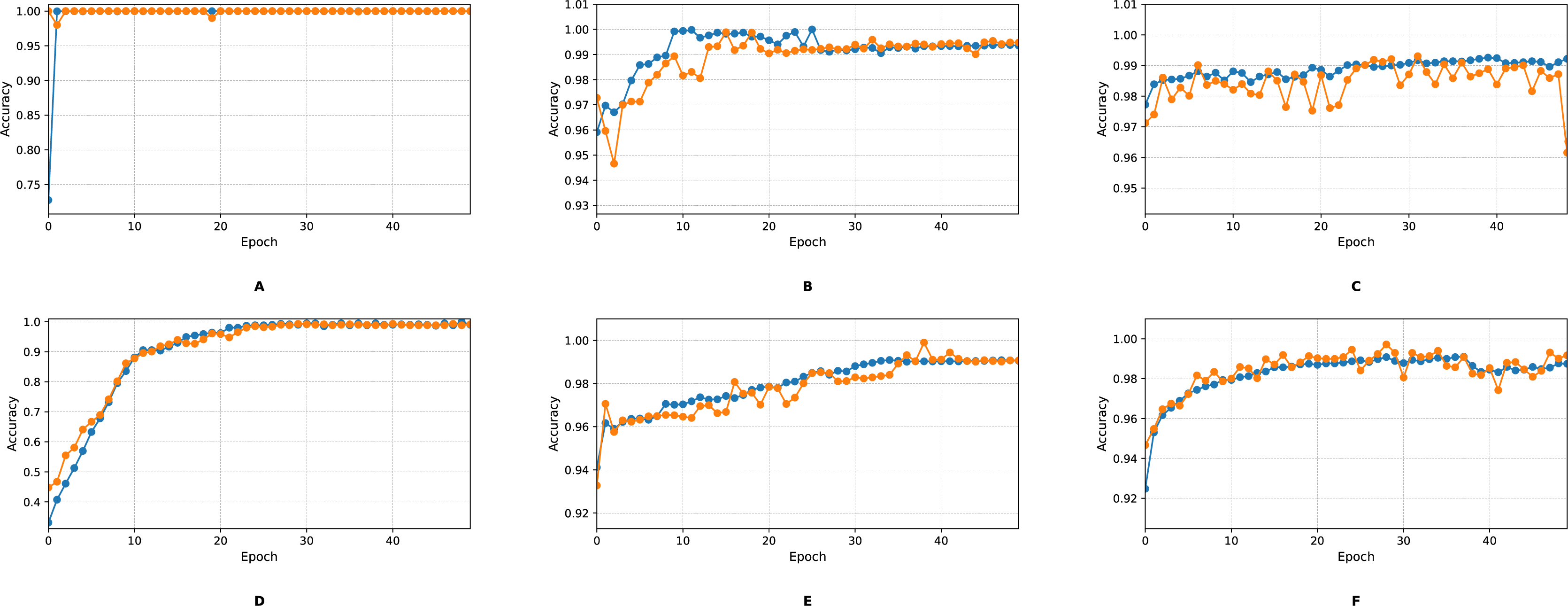
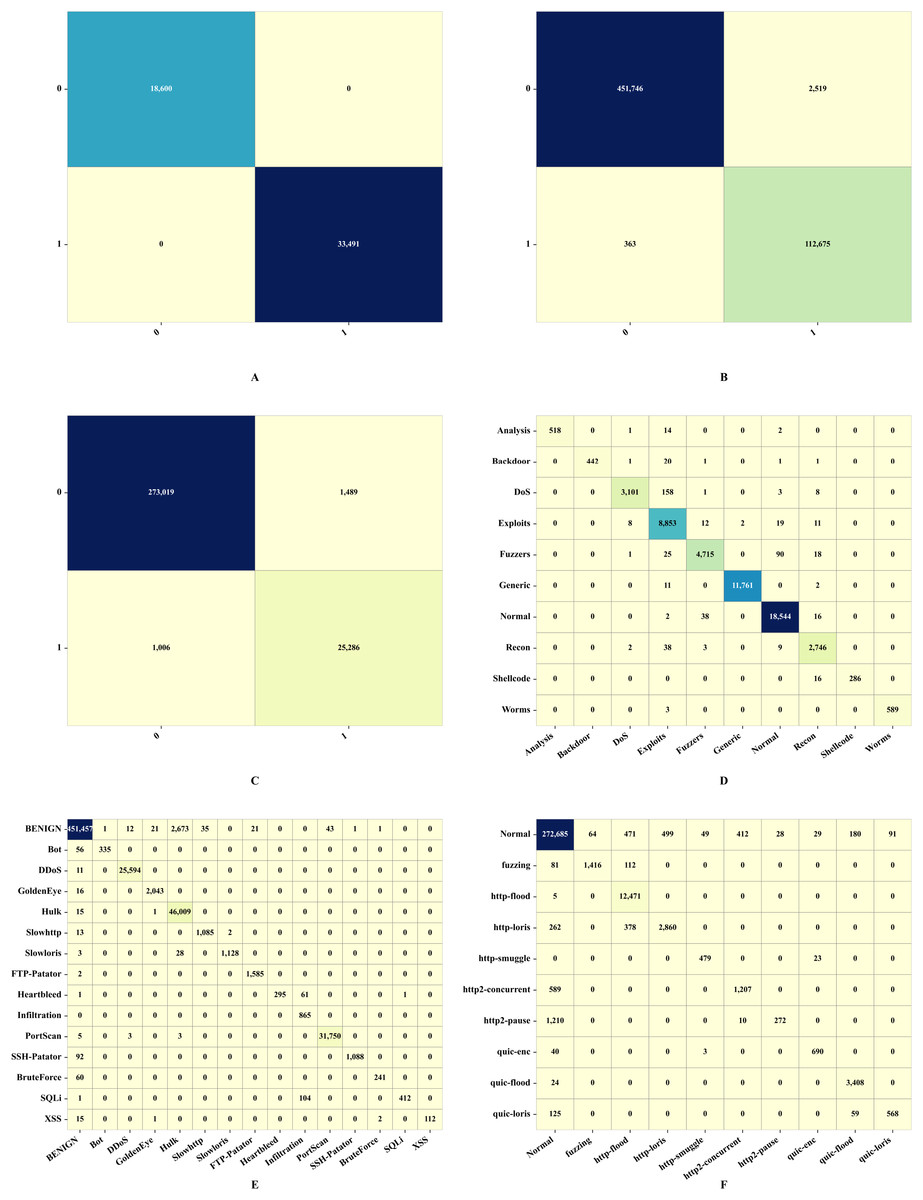
Figure 11: Confusion matrices for the proposed WGAN-GP_IMOA_DA-Ensemble model for binary (A–C) and multiclass (D–F) classification tasks on UNSW-NB15, CIC-IDS2017, and H23Q datasets.
Subplots (A–C) show confusion matrices for binary classification, and (D–F) show confusion matrices for multiclass classification on the UNSW-NB15, CIC-IDS2017, and H23Q datasets.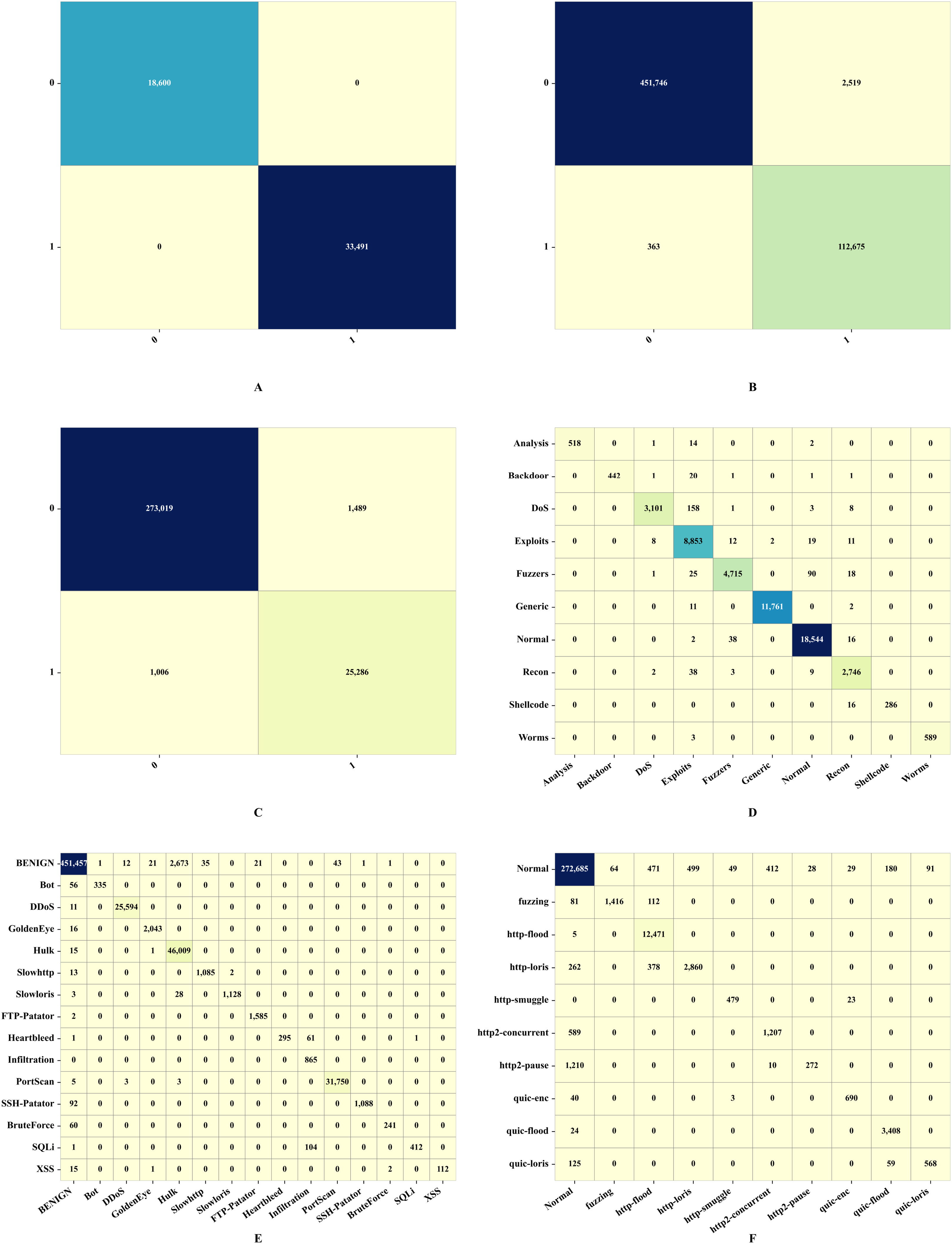
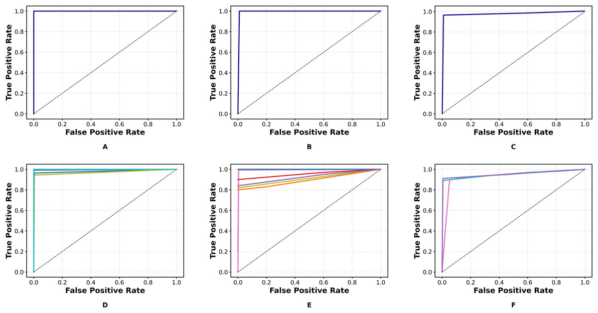
Figure 12: Precision Recall Curve of the proposed WGAN-GP_IMOA_DA-Ensemble model for binary (A–C) and multiclass (D–F) classification tasks on UNSW-NB15, CIC-IDS2017, and H23Q datasets.
Subplots (A–C) display Precision-Recall curves for binary classification, while (D–F) illustrate multiclass classification performance on UNSW-NB15, CIC-IDS2017, and H23Q datasets.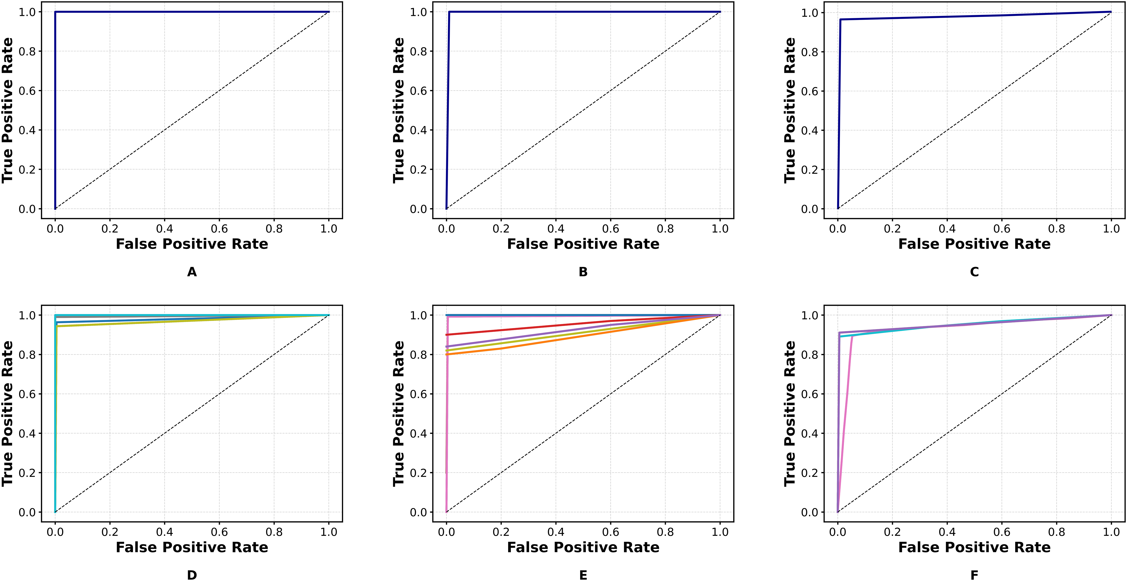
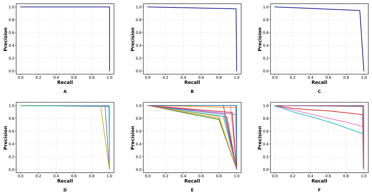
Figure 13: ROC Curve of the proposed WGAN-GP_IMOA_DA-Ensemble model for binary (A–C) and multiclass (D–F) classification tasks on UNSW-NB15, CIC-IDS2017, and H23Q datasets.
Subplots (A–C) present ROC curves for binary classification, and (D–F) present ROC curves for multiclass classification on the UNSW-NB15, CIC-IDS2017, and H23Q datasets.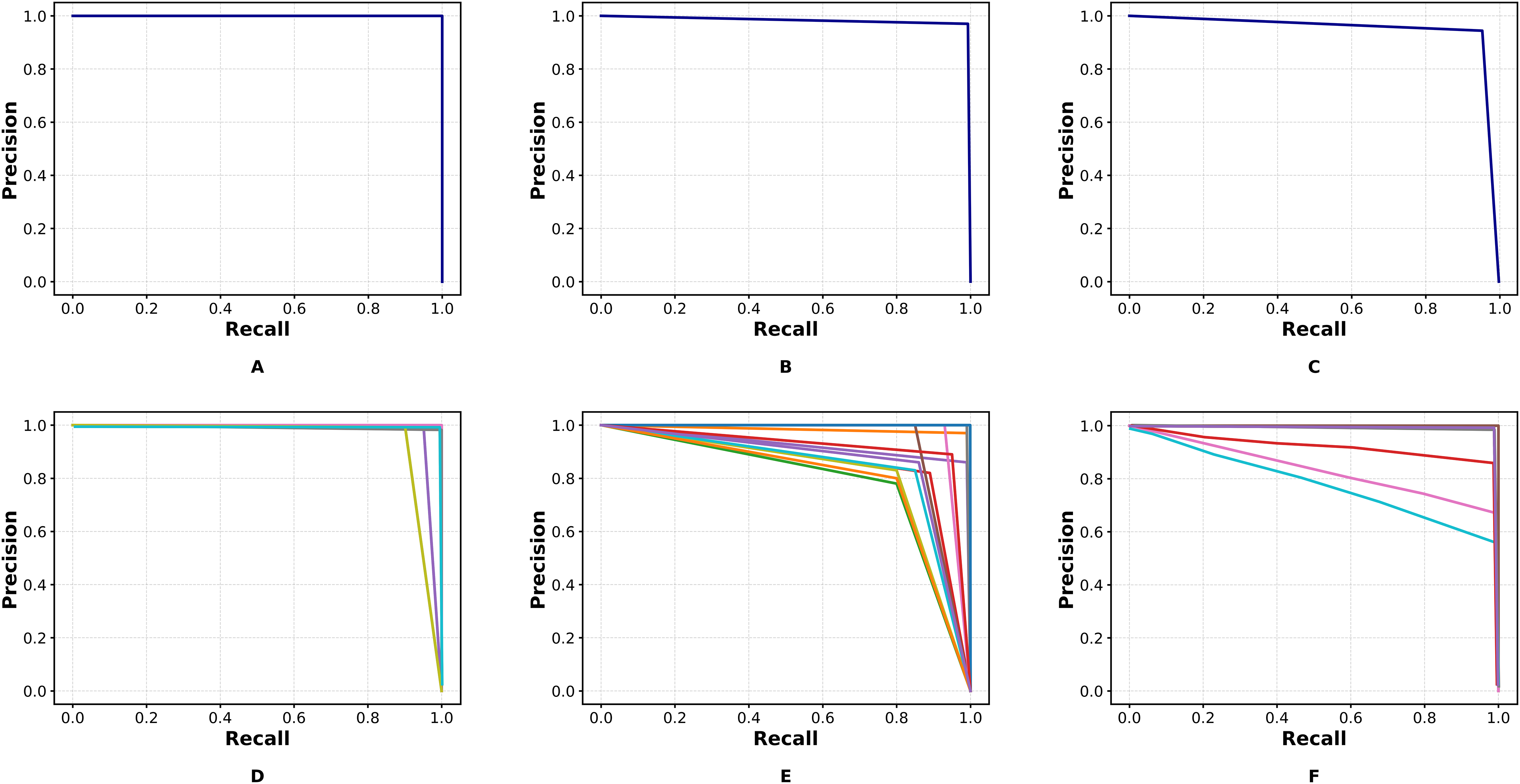
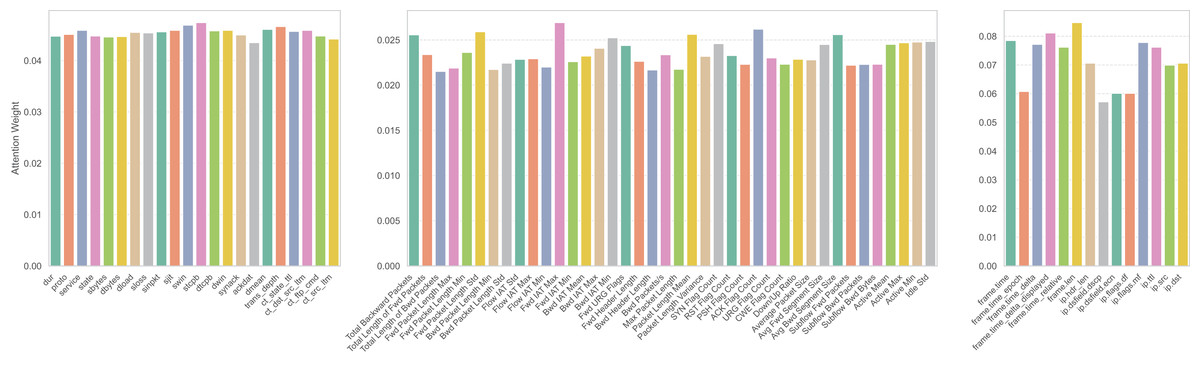
Figure 14: Attention weight plots of the proposed WGAN-GP_IMOA_DA-Ensemble model for binary classification on UNSW-NB15 (A), CIC-IDS2017 (B), and H23Q (C) datasets.
Subplots (A–C) illustrate the attention weights learned by the proposed model during binary classification on the UNSW-NB15, CIC-IDS2017, and H23Q datasets.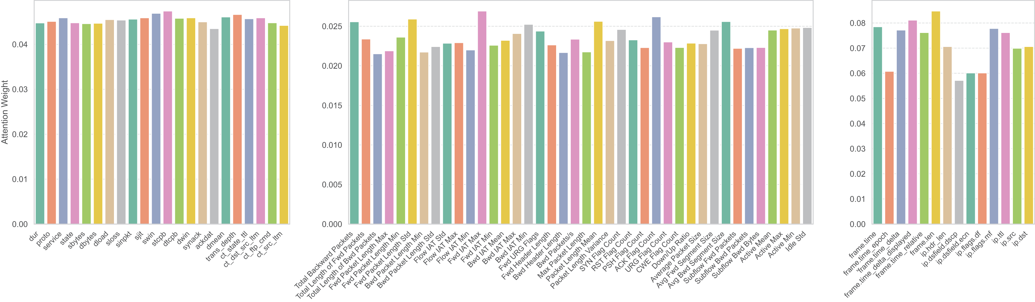
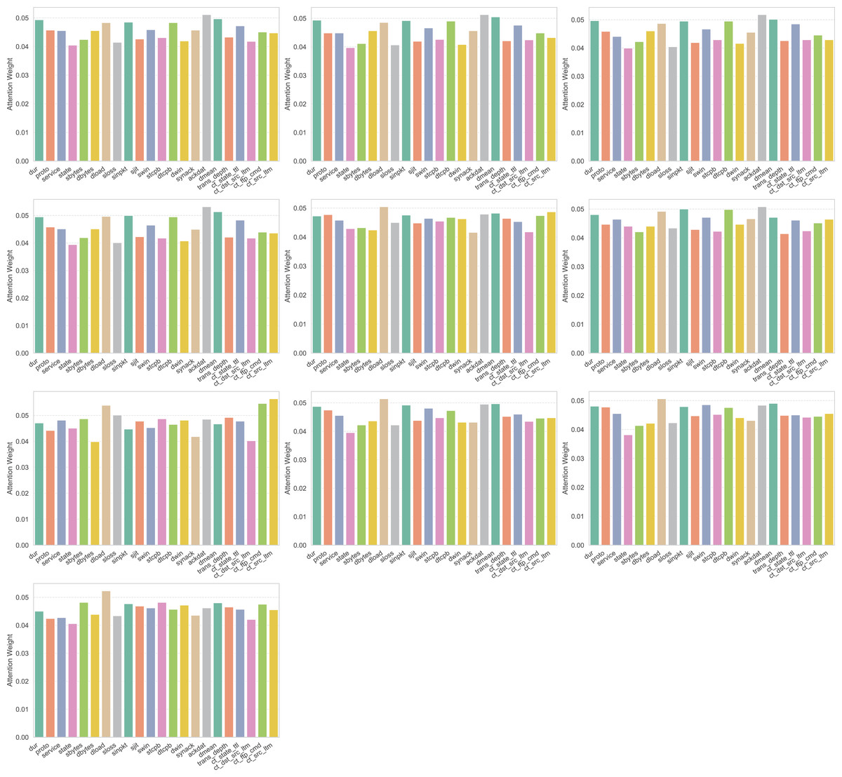
Figure 15: Attention weight distributions for multiclass classification on the UNSW-NB15 dataset across different attack classes.
The plot shows how the proposed model assigns attention weights to different features for each attack class in the UNSW-NB15 dataset during multiclass classification.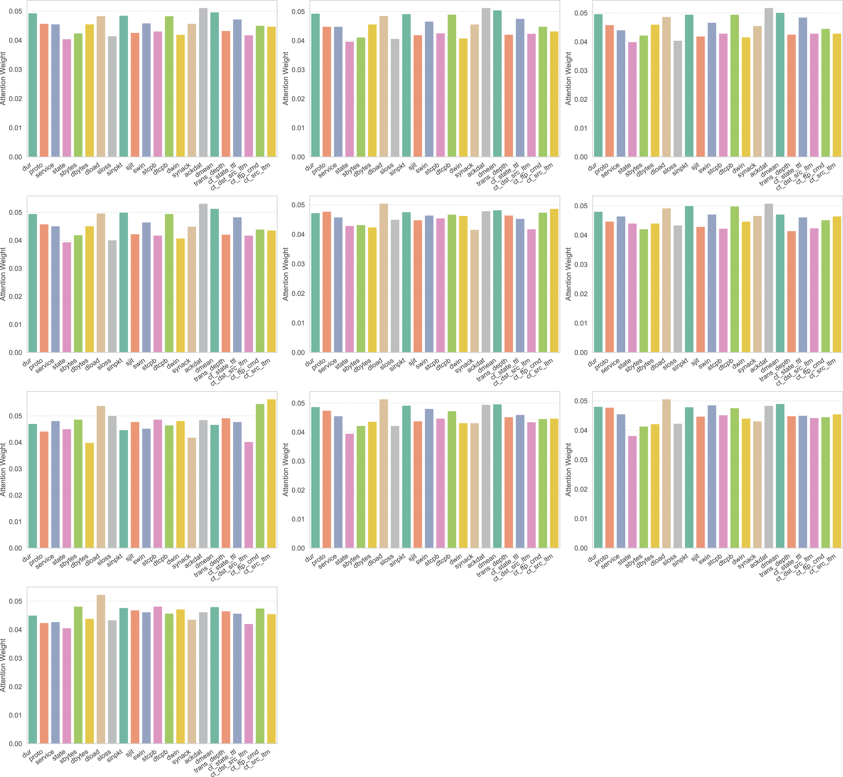
Experimental setup
The experiments were performed on a Dell Latitude laptop with an Intel Core i7-1265U processor, 16 GB of RAM, and Windows 11 Pro (64-bit). Programming was done in Python 3.7, using the Anaconda IDE along with Keras and TensorFlow for deep learning tasks. Microsoft Excel 2021 was utilized to generate comparison charts, and Fotor Pro was used to enhance the quality of images produced by the programming tools.
Experimental design and statistical validity
To ensure the statistical validity and reliability of our evaluation, we adopted the following methodologies across all three datasets.
5-Fold Cross-Validation: All experiments were performed using five-fold stratified cross-validation to ensure class balance in each fold. This approach allowed us to evaluate the consistency and generalizability of model performance across different subsets of data. The metrics accuracy, training time, and memory usage are averaged over the five folds and presented as mean ± standard deviation.
Statistical Significance Testing: To support performance claims, we conducted paired t-tests (α = 0.05) comparing the proposed IMOA-based model with baseline models CNN, LSTM, and FNN. The tests confirmed that the improvements in accuracy are statistically significant in both binary and multiclass settings.
Random Seed Control and Data Partitioning:
For the UNSW-NB15 and CIC-IDS2017 datasets, we utilized the complete datasets with stratified 5-fold cross-validation and ensured no data leakage occurred during preprocessing or splitting. As these datasets are well-structured, we followed consistent fold generation.
For the H23Q dataset, due to its size (~10 million instances), we extracted a stratified random sample of 1,500,000 instances while maintaining class distribution. We used a fixed random seed for repeatability and applied stratified k-fold splitting to avoid bias and ensure no overlap between folds.
These controls ensure that our model evaluations are both statistically grounded and robust across datasets of varying sizes and characteristics.
Performance measures
This section provides an overview of the performance measures applied in this research. The confusion matrix for performance measurement is given in Table 10. The following figures are interpreted alongside the design choices of our framework. Briefly, IMOA reduces redundant and noisy features to improve separability; WGAN-GP addresses class imbalance by synthesizing high-quality minority samples; and the dynamic attention ensemble adaptively weights CNN, LSTM, and FNN learners per instance to leverage their complementary strengths. Together, these components explain why the proposed system consistently outperforms single-model baselines across loss, accuracy, PR/ROC behavior, and confusion matrices.
| Predicted positive | Predicted negative | |
|---|---|---|
| Actual positive | True positive | False negative |
| Actual negative | False positive | True negative |
Loss
The loss function measures the difference between the predicted and actual values. A lower loss indicates that the model’s predictions are closer to the true labels (Bowen et al., 2023). It is calculated for both training and validation sets. Training loss measures the model’s performance on the training data, updated at each epoch. Validation loss measures the model’s performance on the validation set. This research utilizes the Binary cross-entropy (BCE) loss function for binary classification tasks and the Categorical Cross-Entropy (CCE) loss function for multiclass classification tasks (Ahmed et al., 2024).
Binary Cross-Entropy (BCE) loss
It measures the discrepancy between the predicted probability and the actual label. The BCE loss for a dataset of N samples is given by the Eq. (38) (Santos, Miani & de Oliveira Silva, 2024).
(38) where is the true label for the th sample and is the predicted probability of the th sample.
Categorical Cross-Entropy (CCE) loss
It calculates the loss by comparing the predicted probability distribution with the true label’s one-hot encoded representation (Jain et al., 2022). The CCE loss for a dataset of N sample is given by the Eq. (39).
(39) where is the total number of classes, is 1 if the true label is class for the sample and 0 otherwise. is the predicted probability of the sample belonging to class .
Accuracy
Accuracy is defined as the fraction of correct predictions out of the total predictions made (Chinnasamy, Subramanian & Sengupta, 2023b). The formula is
Precision
Precision is the ratio of true positive predictions to the total number of positive predictions made by the model (Subramani & Selvi, 2024). The formula is
Recall
Recall is the ratio of true positive predictions to the total actual positives in the dataset (Subramani & Selvi, 2024). The formula is
F1-score
The F1-score is the harmonic mean of precision and recall, providing a single metric that balances both values (Yesodha et al., 2024).
Precision Recall (PR) curve
A Precision-Recall (PR) Curve is a graphical representation that evaluates the performance of a classification model by illustrating the trade-off between precision and recall at various classification thresholds (Kilichev, Turimov & Kim, 2024).
Receiver Operating Characteristic (ROC) curve
The Receiver Operating Characteristic (ROC) curve is a graphical representation of a classifier’s performance across different threshold settings. It plots the True Positive Rate (TPR) against the False Positive Rate (FPR).
Attention weight plot
This plot shows the attention weights assigned to each feature (or each model’s output component) after the attention mechanism has been applied. By analyzing these weights, one can discern which features or components the model deems most influential in forming its predictions.
The proposed system is trained and tested with the benchmark datasets UNSW-NB15, CIC-IDS2017, and H23Q. The following section explicates the performance of the proposed model applied on the three datasets. The pre-processed datasets are utilized for both binary and multi-class classification tasks.
Results
The proposed model receives input from the pre-processed UNSW-NB15, CIC-IDS2017, and H23Q datasets, which have undergone WGAN-GP data augmentation and IMOA-driven feature selection. The following section analyses various performance measures for the proposed model on the mentioned datasets.
Training and validation loss
This section details the training and validation loss of the WGAN-GP_IMOA_DA_Ensemble model on the mentioned datasets.
Binary Cross Entropy (BCE) loss
The BCE loss curves of the proposed model on the UNSW-NB15 dataset, which are shown in Fig. 9A, start at approximately 0.5 and decrease rapidly to 0.05 by epoch 10. Similarly, the validation loss begins at 0.4 and follows a similar downward trend, converging with the training loss by epoch 10 and stabilizing near 0.01 by epoch 20. The consistent stabilization of both training and validation losses close to 0.01 after epoch 20. However, a notable spike in validation loss occurs at around epoch 20, where it briefly rises to 0.03 before quickly stabilizing again. The BCE loss curves of the proposed model on the CIC-IDS2017 dataset is shown in Fig. 9B. The training loss starts at approximately 0.05 in the first epoch and decreases consistently, stabilizing near 0.02 by epoch 30.
Similarly, the validation loss begins slightly higher, at around 0.06, and follows a similar trend, converging with the training loss by epoch 20 and stabilizing close to 0.02. The BCE loss curves of the proposed model on the H23Q dataset is shown in Fig. 9C. With the training loss starting at approximately 0.06 in the initial epoch and steadily decreased to stabilize near 0.02 after epoch 30. However, the validation loss exhibits notable spikes at several points, such as at epoch 10 (~0.08), epoch 20 (~0.10), and epoch 50 (~0.11), despite following a general downward trend.
In conclusion, the UNSW-NB15 dataset demonstrates the best performance, as its training and validation losses decrease smoothly and stabilize at low values without significant fluctuations. The CIC-IDS2017 dataset performs moderately well, with a stable training loss and slightly noisier validation loss. In contrast, the H23Q dataset shows the least stability, with significant spikes in validation loss despite a steady decrease in training loss.
The DA-Ensemble demonstrates faster and smoother convergence than the baselines because IMOA reduces feature redundancy and WGAN-GP ensures balanced training samples. This leads to lower and more stable validation loss, supporting higher accuracy and F1-scores.
Categorical Cross-Entropy (CCE) loss
The CCE loss curve for the UNSW-NB15 dataset is shown in Fig. 9D. The training loss begins at approximately 0.32 in the initial epoch and decreases steadily, stabilizing close to 0.02 by epoch 30. Similarly, the validation loss starts at 0.30 and follows a comparable downward trend, converging with the training loss around epoch 20 and stabilizing near 0.02 by epoch 40. The CCE loss curve for the CIC-IDS2017 dataset is shown in Fig. 9E. The training loss starts at approximately 0.22 in the first epoch and decreases sharply, reaching 0.05 by epoch 20, and continues to decline gradually, stabilizing near 0.02 by epoch 50. The validation loss follows a similar trajectory, starting at around 0.11, and steadily aligns with the training loss after epoch 20, stabilizing at 0.02 toward the end of training. The CCE loss curve for the H23Q dataset shown in Fig. 9F. The training loss starts at approximately 0.36 in the initial epoch and decreases rapidly to around 0.05 by epoch 10. The validation loss follows a similar trend, starting at approximately 0.22 and aligning closely with the training loss as the epochs progress. Both losses stabilize near 0.02 by epoch 30 and maintain stability throughout the remainder of training, with only minor fluctuations.
Overall, the CIC-IDS2017 dataset demonstrates the best performance. It exhibits steady convergence for both training and validation losses. In comparison, the UNSW-NB15 dataset also performs well, showing rapid convergence and stable validation loss, but its validation loss is slightly higher than that of CIC-IDS2017. The H23Q dataset, while converging, displays slower stabilization and occasional oscillations in validation loss, indicating minor instability.
In multiclass tasks, WGAN-GP balances rare classes, and IMOA selects clearer features, resulting in steadier CCE curves and better results compared to baselines.
The consistently lower and more stable loss of the DA-Ensemble in both binary and multiclass setting arises from (i) IMOA removing redundant/noisy attributes before training, which reduces variance and accelerates convergence, (ii) WGAN-GP rebalancing rare classes to prevent loss spikes from minority misfits, and (iii) dynamic attention dampening over-reliance on any single learner when its confidence is low. Together, these mechanisms reduce overfitting and yield smoother generalization across datasets.
Accuracy curve
This section gives a detailed explanation of the accuracy curve of the proposed WGAN-GP_IMOA_DA_Ensemble model on the datasets UNSW-NB15, CIC-IDS2017, and H23Q with both binary and multi-class classification.
Binary classification
Binary classification refers to the process of categorizing network traffic or system activity into one of two classes: normal (benign) or intrusive (malicious) (Bowen et al., 2023). The accuracy curve of the UNSW-NB15 dataset for binary classification is given in Fig. 10A. The training accuracy reaches a perfect value of 1.0 within the first few epochs, with validation accuracy closely following and stabilizing around the same value. The accuracy curve of the CIC-IDS2017 dataset for binary classification is given in Fig. 10B. The training and validation accuracies steadily improve over the first 20 epochs, stabilizing around 99%. Fluctuations are observed in both curves, particularly during the early and middle epochs of complexity. The accuracy curve of the H23Q dataset for binary classification is given in Fig. 10C. The training accuracy steadily improves and stabilizes around 99%, but the validation accuracy exhibits significant fluctuations throughout the training process.
Overall, the UNSW-NB15 dataset emerges as the best-performing dataset for this binary classification task. The CIC-IDS2017 dataset also performs well, with minor fluctuations. However, the H23Q dataset requires further investigation to address its instability.
The DA-Ensemble reaches higher accuracy levels by combining CNN, LSTM, and FNN strengths through attention weighting, while IMOA and WGAN-GP reduce bias and variance.
Multi-class classification
Multi-class classification involves categorizing network traffic or system activity into one of several predefined classes, each representing a specific type of behavior or attack (More et al., 2024). The accuracy curve of the UNSW-NB15 dataset for multi-class classification is given in Fig. 10D. The training and validation accuracies are stabilizing near-perfect values (close to 1.0) by epoch 30. The accuracy curve of the CIC-IDS2017 dataset for multi-class classification is given in Fig. 10E. It demonstrates slightly lower performance, with training accuracy stabilizing around 99.5% and validation accuracy fluctuating between 98% and 99%. The accuracy curve of the H23Q dataset for multi-class classification is given in Fig. 10F. The training accuracy is stabilizing around 98% but the validation accuracy showing significant fluctuations, particularly in the later epochs.
Overall, UNSW-NB15 is the best-performing dataset for multiclass classification. The CIC-IDS2017 dataset follows as a close second, with strong performance but minor issues in validation stability. The H23Q dataset, however, requires additional preprocessing to improve model stability and generalization. In multiclass settings, balanced samples from WGAN-GP and IMOA-selected features reduce confusion between classes, resulting in consistently higher accuracy.
Accuracy gains are primarily due to IMOA focusing learning on discriminative features, while WGAN-GP mitigates bias toward majority traffic, enabling reliable updates from underrepresented attacks. Dynamic attention then assigns higher weights to CNN on spatially patterned traffic and to LSTM on temporally evolving attacks, which improves accuracy across heterogeneous classes.
Confusion matrix
This section gives details about the confusion matrix of the proposed WGAN-GP_IMOA_DA_Ensemble model on the UNSW-NB15, CIC-IDS2017, and H23Q datasets.
Binary classification
The confusion matrix of the WGAN-GP_IMOA_DA_Ensemble model for binary classification on the UNSW-NB15 dataset is shown in Fig. 11A This confusion matrix indicates that the proposed model achieved perfect classification with no false positives or false negatives. The confusion matrix of the WGAN-GP_IMOA_DA_Ensemble model for binary classification on the CIC-IDS2017 dataset is shown in Fig. 11B. On the CIC-IDS2017 dataset, the model maintains strong performance with 112,675 true positives and 45,146 true negatives, though there are 2,519 false positives and 363 false negatives. The confusion matrix of WGAN-GP_IMOA_DA_Ensemble model for binary classification on the H23Q dataset is shown in Fig. 11C. The model performs well, with 273,019 true positives and 25,286 true negatives, but it has slightly higher false negatives at 1,006 compared to CIC-IDS2017.
Overall, while the UNSW-NB15 dataset shows the highest accuracy, the CIC-IDS2017 dataset provides a more realistic evaluation of the model’s capabilities due to its diversity and complexity. Therefore, the CIC-IDS2017 dataset results highlight the model’s robustness and suitability for practical IDSs.
The DA-Ensemble produces fewer false positives and false negatives, especially for minority classes, because WGAN-GP improves class balance and IMOA enhances class separation.
Multi-class classification
The confusion matrix for multi-class classification of the proposed model on the UNSW-NB15 dataset is shown in Fig. 11D. For normal traffic, there are 18,544 true positives with negligible misclassifications. Among attacks, the model performs well on classes like “Generic” with 11,761 true positives and “Exploits” with 8,853 true positives, indicating strong recognition of these prevalent attack types. However, for minority classes such as “Analysis” and “Backdoor,” the model achieves 518 and 442 true positives, respectively, with some confusion across other classes. Similarly, the “Denial of Service (DoS)” attack class has 3,101 true positives but exhibits minor confusion with “Exploits” and “Fuzzers”.
The confusion matrix for multi-class classification of the proposed model on the CIC-IDS2017 dataset is shown in Fig. 11E. The model performs exceptionally well for the “BENIGN” class, achieving 451,457 true positives with very few false positives. The model also handles high-volume attack classes like “DDoS” and “DoS Hulk” efficiently, with 25,594 and 46,009 true positives, respectively. However, for rare attack types like “Heartbleed” and “Web Attack–SQL Injection,” the true positive counts are 295 and 104, with minor misclassifications into other categories.
The confusion matrix for multi-class classification of the proposed model on the H23Q dataset is shown in Fig. 11F. It shows strong performance for the “Normal” class, with 272,685 true positives and minimal confusion with attack types. Attack types such as “http-flood” and “quic-flood” are also well-classified, with 12,471 and 3,408 true positives, respectively. However, certain attack types like “http2-pause” and “quic-loris” demonstrate lower true positive counts, 272 and 568, respectively, with some confusion across other categories.
Overall, the CIC-IDS2017 dataset offers the best balance between real-world diversity and attack type coverage, showcasing the model’s ability to handle both majority and minority classes effectively. The UNSW-NB15 dataset reflects high accuracy for major classes but struggles more with rare classes, while the H23Q dataset shows strong classification for normal traffic and common attack types but slightly lower performance for rare and complex attacks.
The improved clarity of the diagonals and the reduction in misclassifications for rare classes can be attributed to the proposed components of our framework. Specifically, WGAN-GP generates realistic synthetic samples that mitigate decision-boundary bias against minority classes, while IMOA eliminates redundant features that previously contributed to cross-class confusion. In addition, the dynamic attention mechanism adaptively emphasizes the base learner most suitable for a given instance, further reducing misclassification rates.
Precision-Recall curve
This section provides a detailed explanation of Precision-Recall curve of the WGAN-GP_IMOA_DA_Ensemble model.
Binary classification
For binary classification, the PR curve is generated by plotting precision against recall as the decision threshold. A high area under the curve (AUC) indicates a model that performs well in distinguishing between the positive and negative classes (Yao, Shi & Zhao, 2023).
The PR curve for the UNSW-NB15 dataset in Fig. 12A shows an almost perfect rectangular curve, with precision remaining consistently at 1.0 across all recall values until it sharply drops at the end. The PR curve for the CIC-IDS2017 dataset in Fig. 12B exhibits a minor decline in precision as recall increases, but the overall curve remains close to the top, demonstrating strong model performance. The PR curve for the H23Q dataset in Fig. 12C shows a more pronounced decline in precision as recall increases, resulting in a less rectangular shape.
Overall, based on the PR curves, the proposed model performs best on the UNSW-NB15 dataset, where it achieves near-perfect precision and recall, indicating its robustness in classifying binary labels with minimal errors. The DA-Ensemble maintains high precision even at broad recall ranges, as WGAN-GP addresses class imbalance and IMOA filters for useful features.
Multiclass classification
The PR curves for the UNSW-NB15 dataset in Fig. 12D indicate strong performance across all classes, with average precision (AP) scores ranging from 0.95 to 1.00. The “Normal” and “Generic” classes achieve an AP of 1.00, signifying perfect precision and recall across all thresholds. Minority classes like “Analysis” and “Fuzzers” also perform exceptionally well, with AP values around 0.97. All curves exhibit steep declines only at the extreme right, showcasing strong classification capability until very high recall values.
The PR curves for the CIC-IDS2017 dataset are shown in Fig. 12E. Classes such as “BENIGN,” “DDoS,” and “PortScan” have AP values of 1.00, indicating perfect classification. Certain attack types, including “Web Attack–Brute Force” and “Web Attack–SQL Injection,” show comparatively lower AP scores of 0.79 and 0.80, respectively. The “Bot” and “Heartbleed” classes exhibit moderate AP scores of 0.85 and 0.82, respectively.
The PR curves for the H23Q dataset are shown in Fig. 12F. The “Normal” class achieves an AP of 1.00, showcasing perfect classification performance. Most attack classes, including “http-flood,” “quic-enc,” and “quic-flood,” have AP values of 0.99. However, classes like “fuzzing” and “http-smuggle” display significantly lower AP values of 0.67 and 0.57, respectively.
Overall, the UNSW-NB15 dataset exhibits the best overall performance, with consistently high AP scores across all classes, reflecting a well-trained model and effective feature representation. Minority classes benefit from synthetic balancing and adaptive ensemble weighting, leading to higher average precision across all classes.
Higher AP, especially on minority attacks, stems from WGAN-GP improving positive class coverage at training time, so precision remains high as recall increases. IMOA keeps only signal-bearing attributes, boosting precision at moderate to high recall, while dynamic attention adapts weights per instance, preserving precision under class overlap.
ROC curve
This section gives the details of the ROC curve of both binary and multiclass classification of the proposed WGAN-GP_IMOA_DA_Ensemble on UNSW-NB15, CIC-IDS2017 and H23Q datasets.
Binary classification
The ROC curve for binary classification of the UNSW-NB15 dataset, which is shown in Fig. 13A, is a perfect curve with an AUC score of 1, indicating that the proposed model achieves 100% True Positive Rate (TPR) with no false positives across all thresholds. This implies that the model performs well in distinguishing between benign and malicious traffic on the UNSW-NB15 dataset. The ROC curve for binary classification of the CIC-IDS2017 dataset, which is shown in Fig. 13B, is a perfect diagonal with an AUC score of 1.00, suggesting the model perfectly classifies all instances. The ROC curve for binary classification of the H23Q dataset which is shown in Fig. 13C shows a near-perfect performance but slightly below the previous datasets, with an AUC score of 0.98.
Overall, the proposed model achieves the best results on the UNSW-NB15 and CIC-IDS2017 datasets with binary classification, with AUC scores of 1.00. The performance on the H23Q dataset is slightly lower, with an AUC of 0.98. The DA-Ensemble achieves near-perfect AUC because IMOA prunes noisy features and WGAN-GP balances samples, creating clearer separation between benign and attack traffic.
Multi-class classification
The ROC curve for multi-class classification of the UNSW-NB15 dataset is shown in Fig. 13D. It demonstrates that the model performs exceptionally well on most classes, achieving perfect classification (AUC = 1.00) for classes like Exploits, Generic, Normal, and Worms. The lowest performance is observed for Shellcode, Backdoor, and DoS (AUC = 0.97), which still indicates high separability. The ROC curve for multiclass classification of the CIC-IDS2017 dataset is shown in Fig. 13E. The model achieves excellent performance for major attack types like DDoS, DoS, and infiltration (AUC = 1.00). Performance is slightly lower for Web Attacks, Heartbleed, and Bot, with AUC values ranging from 0.90 to 0.93. The ROC curve for multiclass classification of the H23Q dataset is shown in Fig. 13F. The model shows high performance across all classes, with AUC values between 0.92 and 0.95. Fuzzing exhibits the lowest AUC (0.92), likely due to its complex patterns or overlap with other attack classes. The overall performance is consistent but slightly lower than the other two datasets.
Overall, the UNSW-NB15 dataset demonstrates the best performance, with multiple classes achieving perfect classification (AUC = 1.00) and all other classes maintaining AUC values of 0.97 or higher.
The near-perfect AUC can be attributed to three key factors: (i) IMOA-enhanced feature selection, which improves feature-space separability; (ii) WGAN-GP augmentation, which balances sensitivity to rare attack classes; and (iii) the dynamic attention mechanism, which provides threshold-robust fusion by adaptively reallocating emphasis among CNN, LSTM, and FNN components as operating points vary. Together, these factors account for the consistently higher ROC performance of the proposed model across datasets.
Taken together, the analyses of loss, accuracy, confusion matrices, PR curves, and ROC curves illustrate the stable learning behavior and balanced classification performance of the proposed DA-Ensemble across all datasets. The improvements observed in the evaluation tables and confirmed through statistical tests can be explained by three complementary components: (1) IMOA reduces redundant features and improves class separation, (2) WGAN-GP generates synthetic samples that help balance majority and minority classes, and (3) the dynamic attention ensemble adjusts the weighting of base learners to exploit their different strengths. As a result, DA-Ensemble achieves faster convergence, reliable accuracy, improved recognition of minority classes, and more consistent Precision–Recall and ROC behavior.
Attention weight plot
This section highlights the attention-based visualization of feature importance for binary and multiclass classification in the proposed model, applied to the UNSW-NB15, CIC-IDS2017, and H23Q datasets.
Binary classification
The attention weights for binary classification of the UNSW-NB15 dataset are shown in Fig. 14A, indicate a nearly uniform contribution of features, with slight prominence for features like stcpb (source Transmission Control Protocol (TCP) base), swin (source window size), dmean (mean of destination packets), and trans_depth (transaction depth), which have the highest weights above 0.046. Most features, such as proto, sinpkt, and dtcpb, fall in a narrow range around 0.045, suggesting they also play a significant role in classification. The feature ackdat has the lowest weight (0.0435), indicating a relatively minor influence compared to others.
The attention weight plot for binary classification of the CIC-IDS2017 dataset is shown in Fig. 14B. It demonstrates features such as Fwd Inter-Arrival Time (IAT) Max, Fwd Packet Length Std, Total Backward Packets, and Acknowledgment (ACK) Flag count exhibit significantly higher attention weights. The weights across other features, including Idle Std and Avg Fwd Segment Size, appear evenly distributed with moderate importance. Features including Bwd Packet Length Min and Subflow Fwd Packets received less importance.
The analysis of the H23Q dataset’s attention weights shown in Fig. 14C reveals that frame_len has the highest importance, followed by features like frame_time and frametime_delta_displayed. Network-related features such as ip.ttl, ip.src, and ip.dst also play a moderate role, emphasizing the relevance of protocol-level information. Meanwhile, features like ip.dsfield.dscp and frame.time_epoch have lower attention weights, indicating their relatively minimal contribution to the model’s decision-making.
Multiclass classification
Figure 15 shows the attention weight plots for individual classes of attack for multiclass classification of the proposed model on the UNSW-NB15 dataset. The notable observations are
Analysis: The features such as ackdat and dur have high attention where as dmean, ct_state_ttl, dtcpb received medium attention, and sloss has the least attention.
Backdoor: The model emphasizes ackdat, dmean, dtcpb and dur as key contributors for detecting backdoor attacks, suggesting these features effectively capture patterns associated with unauthorized access.
DoS: Features such as ackdat, dmean and sinpkt, receive higher attention. This aligns with the nature of DoS attacks, where traffic volume is a critical indicator.
Exploits: The focus is distributed among multiple features, including ackdat, dmean sinpkt and dur, indicating the need for a broader feature set to capture the subtleties of Exploits.
Fuzzers: Features such as dload and ct_src_ltm are highlighted, reflecting the importance of data transfer and connection metrics in detecting fuzzing behaviors.
Generic: Protocol-specific features like ackdat and packet-specific attributes like sinpkt stand out, showcasing the model’s ability to identify generic attack patterns using diverse feature sets.
Normal: Traffic attributes like ct_ftp_cmd, ct_src_ltm has higher importance and features such as dbytes and synack has less attention.
Reconnaissance: Features like ackdat, dmean and dload are prioritized, likely due to their role in identifying probing behaviors typical of reconnaissance attacks.
Shellcode: The model emphasizes dload and proto, reflecting their significance in capturing low-level attack behaviors inherent to Shellcode.
Worms: Similar to other classes, dload and dwin receive attention, highlighting their importance in detecting propagation-related activities.
Figure 16 shows the attention weight plots for individual classes of attack for multiclass classification of the proposed model on the CIC-IDS2017 dataset. The notable observations are
-
Benign: Key traffic features such as Active IAT Min, Active Mean, and Total Length of Fwd Packets have higher attention weights, suggesting that these attributes are significant in distinguishing benign traffic patterns.
Bot: Notable features such as Total Backward Packets, Bwd Packets/s, and Avg Fwd Segment Size have high attention weights, indicating their crucial role in identifying bot-related network traffic.
DDoS: Key features such as Total Length of Bwd Packets, Bwd IAT Mean and Average Packet Size have prominent attention weights, reflecting their significance in detecting DDoS attacks.
DoS GoldenEye: Prominent features include Down/Up Ratio, Active Mean and Active Max, which play a critical role in detecting DoS GoldenEye attacks.
DoS Hulk: The DoS Hulk class-specific feature importance plot indicates that Total Length of Fwd Packets, Flow IAT Min, and Max Packet Length are the most critical features.
DoS Slowhttptest: The DoS Slowhttptest class-specific feature importance plot highlights Total Backward Packets, Fwd IAT Max, and Active Max as significant features.
DoS Slowloris: The DoS Slowloris feature importance visualization indicates that Fwd Packet Length Std, Down/Up Ratio, and Flow IAT Min are key distinguishing features.
File Transfer Protocol (FTP)-Patator: The FTP-Patator feature importance analysis highlights that Fwd Packet Length Std, Bwd Packet Length Std, and active mean are significant in identifying this attack type.
Heartbleed: The feature importance analysis reveals that Bwd Packet Length Std, Bwd IAT Min, and Common Weakness Enumeration (CWE) Flag Count are highly weighted.
Infiltration: The feature importance analysis highlights Bwd Packet Length Std, Bwd IAT Min and CWE Flag Count as significant contributors.
Portscan: It reveals that Bwd IAT Max, Bwd IAT Min and Idle Std are key contributors, indicating their relevance in identifying anomalies associated with scanning activity.
Secure Shell (SSH)-Patator: It reveals that Bwd Packet Length Std and Reset (RST) Flag Count are highly influential, indicating their critical role in capturing the nature of brute-force SSH attacks.
Web Attack—SQL Injection: It highlights Bwd Packet Length Std, Bwd IAT Min and CWE Flag Count as dominant contributors.
Web Attack—Cross-Site Scripting (XSS): The top features include Active Min, Total Backward Packets, and Bwd IAT Max, indicating their significance in detecting cross-site scripting attacks.
Web Attack—Brute Force: Active Min, Fwd Packet Length Std, and Bwd IAT Max emerge as the most influential features.
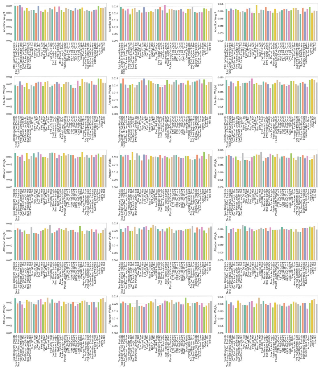
Figure 16: Attention weight distributions for multiclass classification on the CIC-IDS2017 dataset across different attack classes.
The plot shows how the proposed model assigns attention weights to different features for each attack class in the CIC-IDS2017 dataset during multiclass classification.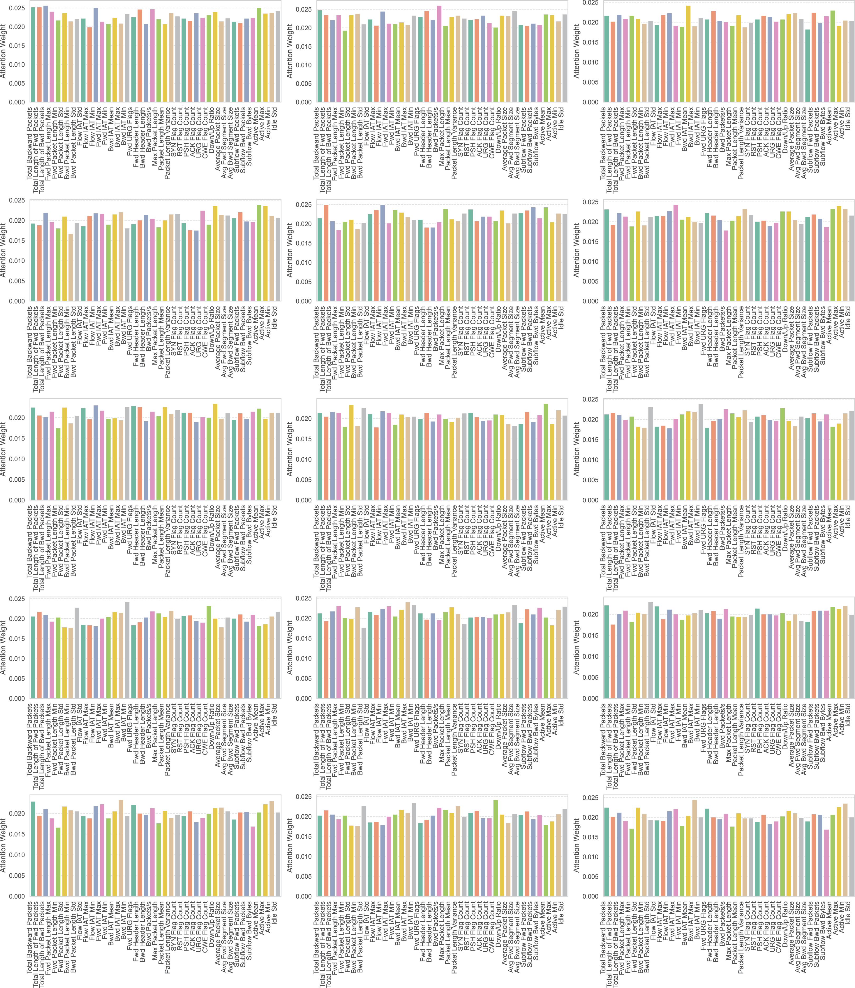
Figure 17 shows the attention weight plots for individual classes of attack for multiclass classification of the proposed model on the H23Q dataset. The notable observations are,
-
Fuzzing: Packet level features such as frame.time,frame.time_epoch and frame.len has high attention.
http2-concurrent: frame.time_relative and ip.ttl among the features receiving higher weights.
http2-pause: frame.len,ip.ttl, and ip.dst are the features having high importance.
http-flood: frame.time_epoch, frame.len, ip.dsfield.ecn and ip.dst are dominant features in deciding the attack http-flood
http-loris: frame.time, frame.len and bip.src are the major contributors in detecting the http-loris attack.
http-smuggle: frame.time_relative, ip.hdr_len and bip.src are the features that receives high attention.
Normal: frame.time, frame.time_relative and ip.dst are the features that receives major attention.
quic-enc: frame.time_epoch, frame.time_relative and frame.len are the major contributing features to detect quic-enc.
quic-flood: frame.time, frame.time_epoch,frame.len and ip.flags.mf has received more attention in detecting quic-flood.
quic-loris: The top features include frame.time,frame.len and ip.dst, indicating their significance in detecting quic-loris attacks.
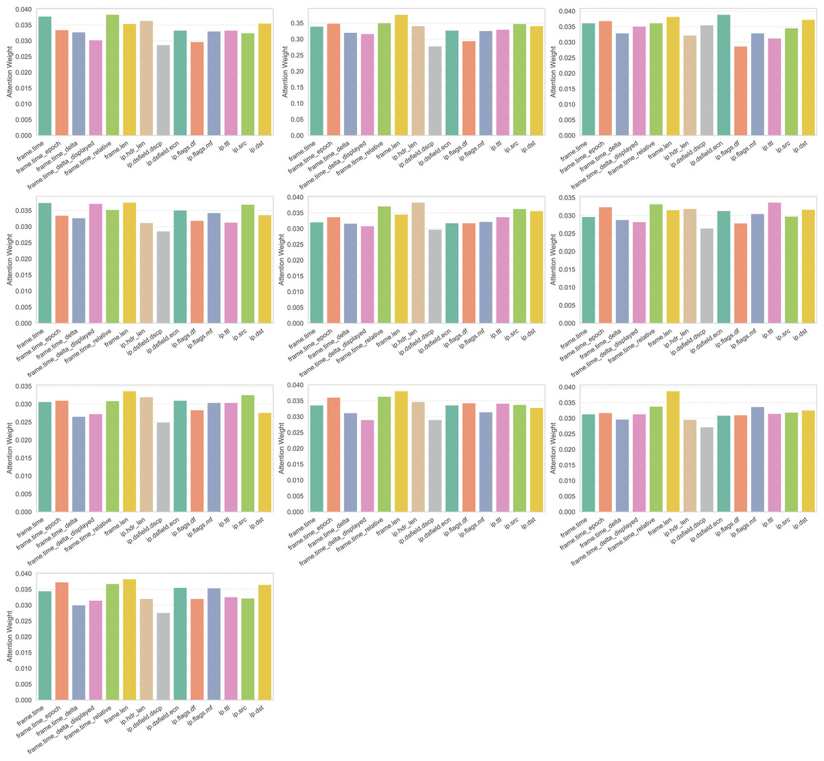
Figure 17: Attention weight distributions for multiclass classification on the H23Q dataset across different attack classes.
The plot shows how the proposed model assigns attention weights to different features for each attack class in the H23Q dataset during multiclass classification.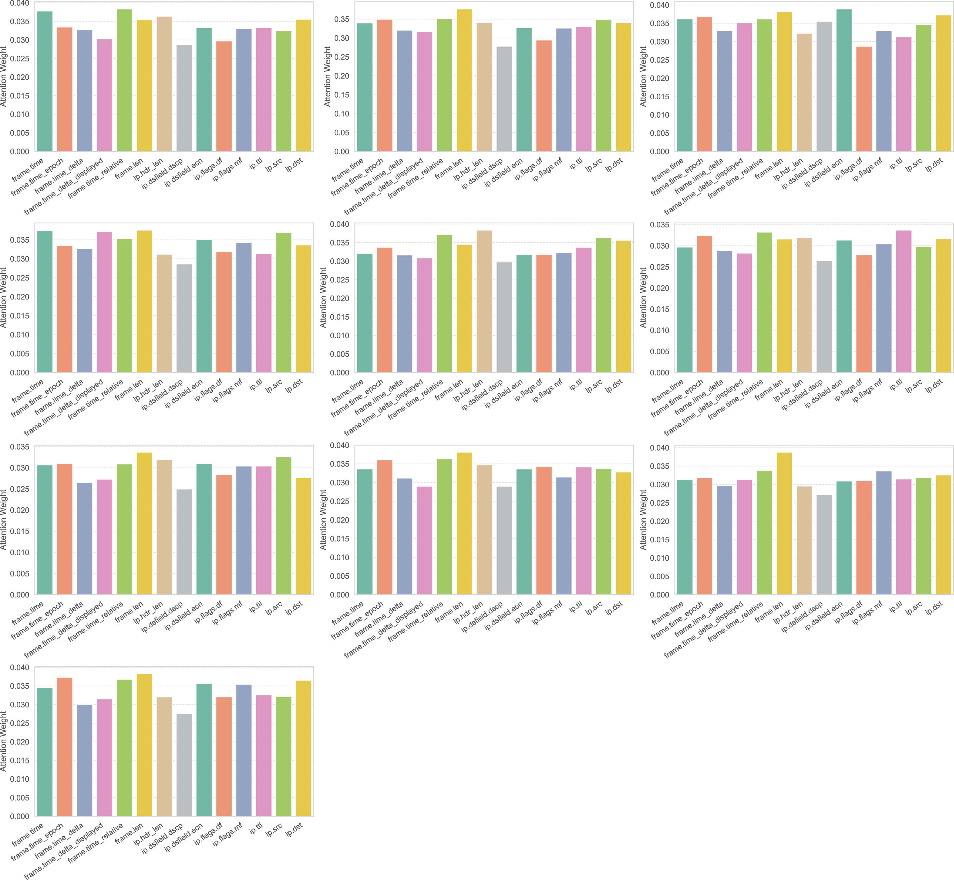
These attention plots from Figs. 14–17 not only highlight which features dominate in each dataset but also explain the superior performance of the DA-Ensemble over baseline methods. By elevating attributes that distinguish minority and complex attack classes, the attention mechanism reduces bias toward majority classes and improves recall on rare categories. When combined with IMOA feature selection, which ensures that only discriminative features enter the model, and WGAN-GP augmentation, which balances the data distribution, the learned attention weights provide a causal explanation for the consistently lower validation loss, higher AUC values, and improved accuracy observed in Figs. 9–13. Thus, Figs. 14–17 provide interpretability that directly supports why the proposed model outperforms existing IDS baselines.
Discussion
Ablation study and component-wise evaluation
To evaluate the contribution of each component in the proposed framework, we conducted an extensive ablation study by progressively integrating the modules such as static ensemble, DA_Ensemble, IMOA-based feature selection, and WGAN-GP-based data augmentation. The results, summarized in Table 11, demonstrate a clear performance improvement at each stage across both binary and multiclass classification tasks on all three datasets. The static ensemble baseline achieved reasonable accuracy, but its performance was limited by feature redundancy and data imbalance. Integrating dynamic attention improved classification consistency and adaptability, while the addition of IMOA further enhanced accuracy and reduced computational overhead by selecting discriminative features. Finally, incorporating WGAN-GP significantly boosted minority class detection, resulting in near-perfect performance metrics (up to 1.00 accuracy, precision, recall, and F1-score) in binary classification and 0.98–0.99 in multiclass settings. Moreover, the proposed model demonstrated favorable trade-offs in terms of training time and memory usage, especially when compared to static and DA_Ensemble configurations, underscoring its practicality for real-world deployment. This ablation analysis confirms that each module contributes meaningfully to the overall performance and justifies the integrated design of the final framework.
| Dataset | Modules | Classification | Accuracy | Precision | Recall | F1-score | Average training time (s) | Average memory |
|---|---|---|---|---|---|---|---|---|
| UNSW-NB15 | Static ensemble | Binary | 0.90 | 0.92 | 0.90 | 0.91 | 5,247.47 ± 28.25 s | 1,012.70 ± 115.70 MiB |
| Multi-class | 0.86 | 0.91 | 0.86 | 0.88 | 34,050.42 ± 56,997.44 s | 815.22 ± 106.29 MiB | ||
| DA_Ensemble | Binary | 0.92 | 0.93 | 0.92 | 0.92 | 5,227.59 ± 207.43 s | 1,255.67 ± 218.77 MiB | |
| Multi-class | 0.88 | 0.93 | 0.88 | 0.90 | 6,020.92 ± 875.14 s | 1,186.44 ± 158.21 MiB | ||
| IMOA + DA_Ensemble | Binary | 0.93 | 0.93 | 0.93 | 0.93 | 4,893.41 ± 112.68 s | 896.91 ± 138.40 MiB | |
| Multi-class | 0.89 | 0.93 | 0.89 | 0.91 | 3,261.76 ± 282.17 s | 1,721.63 ± 102.96 MiB | ||
| WGAN-GP + IMOA + DA_Ensemble (Proposed) | Binary | 1.0 | 1.0 | 1.0 | 1.0 | 5,597.69 ± 1,055.79 s | 1,053.21 ± 217.09 MiB | |
| Multi-class | 0.99 | 0.99 | 0.99 | 0.99 | 514.55 ± 8.35 s | 1,283.10 ± 185.32 MiB | ||
| CIC-IDS2, 017 | Static ensemble | Binary | 0.89 | 0.92 | 0.89 | 0.90 | 87,161.15 ± 2,682.68 s | 3,623.59 ± 426.31 MiB |
| Multi-class | 0.88 | 0.95 | 0.88 | 0.91 | 96,837.78 ± 4,101.75 s | 1,137.00 ± 53.24 MiB | ||
| DA_Ensemble | Binary | 0.90 | 0.93 | 0.90 | 0.91 | 82,206.24 ± 1,265.54 s | 3,852.75 ± 215.90 MiB | |
| Multi-class | 0.89 | 0.95 | 0.89 | 0.91 | 17,370.50 ± 1,722.94 s | 2,552.87 ± 421.04 MiB | ||
| IMOA + DA_Ensemble | Binary | 0.91 | 0.93 | 0.91 | 0.91 | 52,948.40 ± 2,053.89 s | 1,709.12 ± 115.38 MiB | |
| Multi-class | 0.92 | 0.97 | 0.92 | 0.93 | 11,738.25 ± 498.18 s | 1,443.31 ± 348.46 MiB | ||
| WGAN-GP + IMOA + DA_Ensemble (Proposed) | Binary | 0.99 | 1.00 | 0.99 | 0.99 | 60,545.77 ± 2,799.15 s | 1,444.08 ± 441.24 MiB | |
| Multi-class | 0.99 | 0.99 | 0.99 | 0.99 | 139,234.90 ± 17,927.13 s | 1,672.20 ± 242.21 MiB | ||
| H23Q | Static ensemble | Binary | 0.87 | 0.93 | 0.87 | 0.89 | 18,845.71 ± 1,710.39 s | 845.10 ± 110.74 MiB |
| Multi-class | 0.88 | 0.97 | 0.88 | 0.92 | 36,784.18 ± 1,525.64 s | 1,652.21 ± 47.61 MiB | ||
| DA_Ensemble | Binary | 0.91 | 0.94 | 0.91 | 0.92 | 23,622.68 ± 693.11 s | 1,323.90 ± 198.70 MiB | |
| Multi-class | 0.89 | 0.97 | 0.89 | 0.92 | 5,852.00 ± 236.48 s | 1,340.00 ± 208.85 MiB | ||
| IMOA + DA_Ensemble | Binary | 0.92 | 0.94 | 0.92 | 0.92 | 10,009.53 ± 535.43 s | 2,106.70 ± 85.24 MiB | |
| Multi-class | 0.90 | 0.97 | 0.90 | 0.93 | 4,377.13 ± 144.94 s | 1,309.69 ± 176.29 MiB | ||
| WGAN-GP + IMOA + DA_Ensemble (Proposed) | Binary | 0.99 | 0.99 | 0.99 | 0.99 | 9,759.59 ± 775.36s | 1,497.67 ± 77.17 MiB | |
| Multi-class | 0.98 | 0.98 | 0.98 | 0.98 | 2,039.61 ± 234.18 s | 1,488.80 ± 140.32 MiB |
Statistical significance analysis
To ensure that the performance improvements achieved by the proposed WGAN-GP_IMOA_DA-Ensemble model are not due to random variation, we conducted a series of paired t-tests comparing its classification accuracy against three baseline models, such as CNN, LSTM, and FNN across both binary and multiclass settings for all datasets. The results, summarized in Table 12, show that all comparisons yielded p-values below 0.05, confirming that the improvements are statistically significant. In many cases, the p-values were far smaller like less than 0.001, accompanied by extremely high t-statistics, which provide strong evidence of consistent and reproducible improvements.
| Dataset | Classification | Baseline vs. proposed | t-statistic | p-value | Statistically significant (p < 0.05) |
|---|---|---|---|---|---|
| UNSW-NB15 | Binary | CNN vs. DA-Ensemble | 1.7404557886333356 | 0.01567545111738706 | Yes |
| LSTM vs. DA-Ensemble | 1,563.7300000004682 | 1.0034667664427704e-12 | Yes | ||
| FNN vs. DA-Ensemble | 3,294.555746438036 | 5.092881150858561e-14 | Yes | ||
| Multiclass | CNN vs. DA-Ensemble | 12.889258189933278 | 0.0002089343865805691 | Yes | |
| LSTM vs. DA-Ensemble | 6.699023290065787 | 0.00258341180114001 | Yes | ||
| FNN vs. DA-Ensemble | 11.97626398351866 | 0.0002785766624558316 | Yes | ||
| CIC-IDS2017 | Binary | CNN vs. DA-Ensemble | 32.31013064432767 | 5.470512987977092e-0 | Yes |
| LSTM vs. DA-Ensemble | 5.810480547643236 | 0.0043658384460866255 | Yes | ||
| FNN vs. DA-Ensemble | 13.253003293334746 | 0.0001873213167449350 | Yes | ||
| Multiclass | CNN vs. DA-Ensemble | 83.06522046184398 | 1.259084449585072e-07 | Yes | |
| LSTM vs. DA-Ensemble | 5.55420830644023 | 0.005142676188209267 | Yes | ||
| FNN vs. DA-Ensemble | 9.047216336434865 | 0.0008270310181249053 | Yes | ||
| H23Q | Binary | CNN vs. DA-Ensemble | 82.5118686776108 | 1.2931842692845362e-07 | Yes |
| LSTM vs. DA-Ensemble | 16.75371119090979 | 7.438098006382559e-05 | Yes | ||
| FNN vs. DA-Ensemble | 108.40719208481883 | 4.3418272910447173e-08 | Yes | ||
| Multiclass | CNN vs. DA-Ensemble | 7.852240113549909 | 0.0014210846958986809 | Yes | |
| LSTM vs. DA-Ensemble | 4.5188955914851805 | 0.010667313739832018 | Yes | ||
| FNN vs. DA-Ensemble | 13.997412174613357 | 0.0001511212440940260 | Yes |
For the UNSW-NB15 dataset, the DA-Ensemble achieved highly significant improvements in binary classification, outperforming the LSTM baseline with a t value of 1,563.73 and a p value of 1.00 × 10⁻¹² and the FNN baseline with a t value of 3,294.56 and a p value of 5.09 × 10⁻¹⁴. In multiclass classification, the DA-Ensemble again demonstrated clear statistical significance, such as against CNN with a t value of 12.89 and a p value of 2.09 × 10⁻⁴. On the CIC-IDS2017 dataset, the results were equally impressive. In binary classification, the DA-Ensemble significantly outperformed CNN with a t value of 32.31 and a p value of 5.47 × 10⁻⁹, LSTM with a t value of 5.81 and a p value of 4.37 × 10⁻³, and FNN with a t value of 13.25 and a p value of 1.87 × 10⁻⁴. In multiclass settings, the DA-Ensemble consistently outperformed all baselines, with strong results such as CNN vs. DA-Ensemble with a t value of 83.07 and a p value of 1.26 × 10⁻⁷.
For the H23Q dataset, statistical significance was again observed across both tasks. In binary classification, the DA-Ensemble demonstrated highly significant improvements, such as against the FNN baseline, with a t value of 108.41 and a p value of 4.34 × 10⁻⁸. Multiclass classification results also confirmed the robustness of the approach, with examples including CNN vs. DA-Ensemble, with a t value of 7.85 and a p value of 1.42 × 10⁻³, and FNN vs. DA-Ensemble, with a t value of 13.99 and a p value of 1.51 × 10⁻⁴.
Collectively, these findings emphasize two key points. First, the consistently low p-values across three benchmark datasets and both binary and multiclass tasks confirm that the observed improvements are not due to random chance. Second, the size of the t-statistics highlights that the gains are both statistically significant and practically meaningful. Overall, this thorough statistical validation offers strong confidence in the reliability, robustness, and generalizability of the DA-Ensemble framework for intrusion detection. Although this study focuses on t-tests and p-values, future work could include confidence intervals and effect size measures such as Cohen’s d to enhance the statistical analysis further.
Validation of the research hypothesis through performance metrics
To evaluate our research hypothesis, we assessed the performance of the proposed IDS framework using standard classification metrics such as accuracy, precision, recall, F1-score, and confusion matrix. These metrics were used to examine whether the IMOA_WGAN-GP_DA_Ensemble model effectively enhances performance, particularly for underrepresented attack classes. The results obtained across all datasets demonstrate consistent improvements in classification performance for both binary and multiclass settings, supporting the validity of the proposed approach.
Computational performance
To assess the feasibility and efficiency of the proposed IDS model, we performed detailed experiments measuring the computational cost, including average training time and memory usage, across three benchmark datasets: UNSW-NB15, CIC-IDS2017, and H23Q. The proposed WGAN-GP_IMOA_DA_Ensemble was compared to baseline deep learning models (CNN, LSTM, and FNN), each integrated with WGAN-GP and IMOA to ensure a fair comparison.
The results, summarized in Table 13, show that the proposed ensemble incurs higher training time and moderate memory overhead due to the attention mechanism and multi-model integration. However, this trade-off is justified by its consistently better classification performance across datasets, making it computationally feasible for real-world IDS deployment.
| Dataset | Modules | Classification | Accuracy | Average training time (s) | Average memory |
|---|---|---|---|---|---|
| UNSW-NB15 | WGAN-GP + IMOA + CNN | Binary | 0.9590 ± 0.0815 | 904.67 ± 26.81 s | 839.07 ± 247.97 MiB |
| Multi-class | 0.8393 ± 0.0241 | 457.50 ± 10.39 s | 1,211.23 ± 138.86 MiB | ||
| WGAN-GP + IMOA + LSTM | Binary | 0.9700 ± 0.0000 | 4,991.16 ± 246.31 s | 879.13 ± 215.07 MiB | |
| Multi-class | 0.8489 ± 0.0402 | 2,646.59 ± 103.84 s | 1,224.04 ± 151.46 MiB | ||
| WGAN-GP + IMOA + FNN | Binary | 0.9800 ± 0.0000 | 480.41 ± 20.58 s | 828.51 ± 281.62 MiB | |
| Multi-class | 0.9203 ± 0.0132 | 221.67 ± 4.82 s | 1,129.61 ± 292.43 MiB | ||
| WGAN-GP + IMOA + DA_Ensemble (Proposed) | Binary | 1.0000 ± 0.0000 | 5,597.69 ± 1,055.79 s | 1,053.21 ± 217.09 MiB | |
| Multi-class | 0.9901 ± 0.0038 | 514.55 ± 8.35 s | 1,283.10 ± 185.32 MiB | ||
| CIC-IDS2017 | WGAN-GP + IMOA + CNN | Binary | 0.8829 ± 0.0022 | 8,588.95 ± 725.30 s | 1,169.48 ± 470.16 MiB |
| Multi-class | 0.8685 ± 0.0029 | 26,282.20 ± 479.48 s | 1,516.99 ± 265.11 MiB | ||
| WGAN-GP + IMOA + LSTM | Binary | 0.8975 ± 0.0363 | 57,653.00 ± 3,068.33 s | 1,328.84 ± 463.46 MiB | |
| Multi-class | 0.8733 ± 0.0419 | 227,192.97 ± 169,782.02 s | 1,563.88 ± 254.57 MiB | ||
| WGAN-GP + IMOA + FNN | Binary | 0.9464 ± 0.0039 | 3,804.13 ± 86.41 s | 1,335.71 ± 463.04 MiB | |
| Multi-class | 0.9412 ± 0.0105 | 8,532.20 ± 785.83 s | 1,575.86 ± 250.06 MiB | ||
| WGAN-GP + IMOA + DA_Ensemble (Proposed) | Binary | 0.9918 ± 0.0052 | 60,545.77 ± 2,799.15 s | 1,444.08 ± 441.24 MiB | |
| Multi-class | 0.9906 ± 0.0005 | 139,234.90 ± 17,927.13 s | 1,672.20 ± 242.21 MiB | ||
| H23Q | WGAN-GP + IMOA + CNN | Binary | 0.8247 ± 0.0029 | 1,853.33 ± 73.06 s | 1,307.13 ± 197.40 MiB |
| Multi-class | 0.9332 ± 0.0027 | 497.34 ± 145.28 s | 1,488.62 ± 170.04 MiB | ||
| WGAN-GP + IMOA + LSTM | Binary | 0.8719 ± 0.0122 | 9,579.01 ± 284.30 s | 1,331.18 ± 118.14 MiB | |
| Multi-class | 0.9424 ± 0.0123 | 2,600.65 ± 1,077.18 s | 1,500.22 ± 145.61 MiB | ||
| WGAN-GP + IMOA + FNN | Binary | 0.9126 ± 0.0000 | 1,130.35 ± 59.30 s | 1,216.68 ± 197.20 MiB | |
| Multi-class | 0.9126 ± 0.0000 | 288.00 ± 113.86 s | 1,317.63 ± 111.91 MiB | ||
| WGAN-GP + IMOA + DA_Ensemble (Proposed) | Binary | 0.9806 ± 0.0013 | 9,759.59 ± 775.36 s | 1,497.67 ± 77.17 MiB | |
| Multi-class | 0.9800 ± 0.0096 | 2,039.61 ± 234.18 s | 1,488.80 ± 140.32 MiB |
Moving beyond computational cost, we next evaluate the classification performance.
Classification performance
The classification report for the binary classification of the proposed model on UNSW-NB15, CIC-IDS2017, and H23Q datasets is shown in Table 14. For UNSW-NB15, the model achieves perfect performance (1.00 for all metrics), indicating perfect classification. In CIC-IDS2017, the model maintains a strong overall accuracy of 0.99, with near-perfect metrics for the benign class. In contrast, the attack class shows slightly lower precision of 0.98 due to some false positives. The H23Q dataset also achieves 0.99 accuracy, with perfect metrics for the normal class but slightly lower precision of 0.94 and an F1-score of 0.95 for the attack class.
| Dataset | Class | Precision | Recall | F1-score | Support |
|---|---|---|---|---|---|
| UNSW-NB15 | 0 | 1.00 | 1.00 | 1.00 | 18,600 |
| 1 | 1.00 | 1.00 | 1.00 | 33,492 | |
| Macro average | 1.00 | 1.00 | 1.00 | 52,092 | |
| Weighted average | 1.00 | 1.00 | 1.00 | 52,092 | |
| Accuracy | 1.00 | 52,092 | |||
| CIC-IDS2017 | 0 | 1.00 | 0.99 | 1.00 | 454265 |
| 1 | 0.98 | 1.00 | 0.99 | 113,038 | |
| Macro average | 0.99 | 1.00 | 0.99 | 567,303 | |
| Weighted average | 0.99 | 0.99 | 0.99 | 567,303 | |
| Accuracy | 0.99 | 567,303 | |||
| H23Q | 0 | 1.00 | 0.99 | 1.00 | 274,508 |
| 1 | 0.94 | 0.96 | 0.95 | 26,292 | |
| Macro average | 0.97 | 0.98 | 0.97 | 300,800 | |
| Weighted average | 0.99 | 0.99 | 0.99 | 300,800 | |
| Accuracy | 0.99 | 300,800 | |||
The performance comparison of the proposed model with benchmark models on binary classification is provided in Table 15. For the UNSW-NB15 dataset, it achieves a perfect 100% across accuracy, precision, recall, and F1-score, outperforming models like OHDNN + Enhanced Conditional Random Field (ECRF) (98.30% accuracy) and CNN + LSTM (93.21% accuracy). Similarly, for the CIC-IDS2017 dataset, the proposed model reaches 99% in all metrics, surpassing benchmark models such as Naïve Bayes (NB)+Elliptic Envelop (EE), which achieved 98.59% accuracy, and Hybrid convolutional neural network + Bidirectional Long Short-Term Memory (HCNN + BLSTM), which scored 98% accuracy but lower precision and recall. Although models like Sample Generation Model (SGM)+CNN and Tree-CNN+Simple Random Sampling (SRS) demonstrate strong performance, they are outperformed in key metrics by the proposed model. Since the H23Q dataset is new, there is no direct performance comparison available, making this work a pioneering contribution in this area.
| Model | Year | Accuracy | Precision | Recall | F1-score |
|---|---|---|---|---|---|
| UNSW-NB15 binary classification | |||||
| K-NN (Kareem et al., 2022) | 2022 | 97.01% | 81.53% | ||
| MMultiSVM (Turukmane & Devendiran, 2024) | 2024 | 97.53% | 97.67% | 98.94% | 97.99% |
| CNN + LSTM (Meliboev, Alikhanov & Kim, 2022) | 2022 | 87.60% | 85.50% | 90.60% | 88% |
| HCNN + ALSTM (Ragab & Sabir, 2022) | 2022 | 92.87% | 97.33% | 77.53% | 72.53% |
| CNN + LSTM (Altunay & Albayrak, 2023) | 2023 | 93.21% | |||
| CNN + LSTM + AES (Thilagam & Aruna, 2023) | 2023 | 96.99% | 95.45% | ||
| OHDNN + ECRF (Karthic & Kumar, 2023) | 2023 | 98.30% | 97.50% | 96.70% | 97.10% |
| Proposed model | 2025 | 100% | 100% | 100% | 100% |
| CIC-IDS2017 binary classification | |||||
| LSTM (Hanafi et al., 2023) | 2024 | 98.36% | 96.68% | 97.91% | 97.29% |
| HCNN + ALSTM (Ragab & Sabir, 2022) | 2022 | 97.62% | 97.26% | 97.25% | 99% |
| HCNN + BLSTM (Bowen et al., 2023) | 2023 | 98% | 86% | 84% | 81% |
| GAN + CNN + BiLSTM (Li, Li & Li, 2023) | 2023 | 96.32% | 96.55% | 95.38% | 96.04% |
| NB + EE (Vishwakarma & Kesswani, 2023) | 2023 | 98.59% | 95.40% | 97.51% | 96.44% |
| HBO + ANN (Chinnasamy, Subramanian & Sengupta, 2023a) | 2023 | 97.60% | |||
| Proposed model | 2025 | 99% | 99% | 99% | 99% |
The classification reports for the multi-class classification of the proposed model on UNSW-NB15, CIC-IDS2017, and H23Q datasets are given in Table 16. For UNSW-NB15, the model achieves an impressive 0.99 accuracy, with near-perfect metrics across most classes. Attack “Generic” achieves 1.00 precision, recall, and F1-score, indicating flawless classification. However, attacks like ”Backdoor“ and “Shellcode” show slightly lower recall (0.95), suggesting some false negatives. The macro average metrics (0.99 precision, 0.98 recall, 0.98 F1-score) indicate balanced performance across all classes.
| Dataset | Class | Precision | Recall | F1-score | Support | |
|---|---|---|---|---|---|---|
| UNSW-NB15 | Analysis | 1.00 | 0.97 | 0.98 | 535 | |
| Backdoor | 1.00 | 0.95 | 0.97 | 466 | ||
| DoS | 1.00 | 0.95 | 0.97 | 3,271 | ||
| Exploits | 0.97 | 0.99 | 0.98 | 8,905 | ||
| Fuzzers | 0.99 | 0.97 | 0.98 | 4,849 | ||
| Generic | 1.00 | 1.00 | 1.00 | 11,774 | ||
| Normal | 0.99 | 1.00 | 1.00 | 18,600 | ||
| Reconnaissance | 0.97 | 0.98 | 0.98 | 2,798 | ||
| Shellcode | 1.00 | 0.95 | 0.97 | 302 | ||
| Worms | 1.00 | 0.99 | 1.00 | 592 | ||
| Macro average | 0.99 | 0.98 | 0.98 | 52,092 | ||
| Weighted average | 0.99 | 0.99 | 0.99 | 52,092 | ||
| Accuracy | 0.99 | 52,092 | ||||
| CIC-IDS2017 | BENIGN | 1.00 | 0.99 | 1.00 | 454265 | |
| Bot | 1.00 | 0.86 | 0.92 | 391 | ||
| DDoS | 1.00 | 1.00 | 1.00 | 25,605 | ||
| DoS GoldenEye | 0.99 | 0.99 | 0.99 | 2,059 | ||
| DoS Hulk | 0.95 | 1.00 | 0.97 | 46,025 | ||
| DoS Slowhttptest | 0.95 | 0.99 | 0.97 | 1,100 | ||
| DoS slowloris | 1.00 | 0.97 | 0.99 | 1,159 | ||
| FTP-Patator | 0.99 | 1.00 | 0.99 | 1,587 | ||
| Heartbleed | 1.00 | 0.82 | 0.90 | 358 | ||
| Infiltration | 0.84 | 1.00 | 0.91 | 865 | ||
| PortScan | 1.00 | 1.00 | 1.00 | 31,761 | ||
| SSH-Patator | 1.00 | 0.92 | 0.96 | 1,180 | ||
| Web Attack-Brute Force | 0.99 | 0.80 | 0.88 | 301 | ||
| Web Attack-Sql Injection | 1.00 | 0.80 | 0.89 | 517 | ||
| Web Attack-XSS | 1.00 | 0.86 | 0.93 | 130 | ||
| Macro Average | 0.98 | 0.93 | 0.95 | 567,303 | ||
| Weighted Average | 0.99 | 0.99 | 0.99 | 567,303 | ||
| Accuracy | 0.99 | 567,303 | ||||
| H23Q | Normal | 0.99 | 0.99 | 0.99 | 274,508 | |
| fuzzing | 0.96 | 0.88 | 0.92 | 1,609 | ||
| http-flood | 0.93 | 1.00 | 0.96 | 12,476 | ||
| http-loris | 0.85 | 0.82 | 0.83 | 3,500 | ||
| http-smuggle | 0.90 | 0.95 | 0.93 | 502 | ||
| http2-concurrent | 0.74 | 0.67 | 0.70 | 1,796 | ||
| http2-pause | 0.91 | 0.18 | 0.30 | 1,492 | ||
| Quic-enc | 0.93 | 0.94 | 0.94 | 733 | ||
| Quic-flood | 0.93 | 0.99 | 0.96 | 3,432 | ||
| Quic-loris | 0.86 | 0.76 | 0.81 | 752 | ||
| Macro average | 0.90 | 0.82 | 0.83 | 300,800 | ||
| Weighted average | 0.98 | 0.98 | 0.98 | 300,800 | ||
| Accuracy | 0.98 | 300,800 | ||||
For CIC-IDS2017, with an overall 0.99 accuracy, the model performs exceptionally well for the attack types like “DDoS” and “PortScan” (all scoring 1.00 F1-score). However, attack classes like “Bot” and “Heartbleed” have lower recall (0.86 and 0.82, respectively), indicating some missed detections. Additionally, “Web Attack” variants show variability in performance, with “Web Attack–XSS” achieving an F1-score of 0.93, while “Web Attack—SQL Injection” and “Web Attack–Brute Force” score lower (0.89 and 0.88). The macro average metrics (0.98 precision, 0.93 recall, 0.95 F1-score) highlight slightly reduced performance for minority classes compared to the majority.
For H23Q, the model achieves 0.98 accuracy. The “Normal” traffic is classified with high precision and recall (0.99), minority classes like “http2-pause” and “http2-concurrent” perform poorly, with F1-scores of 0.30 and 0.70, respectively, due to low recall. Attack types like “http-loris” and “quic-loris” also show reduced performance, with F1-scores of 0.83 and 0.81. The macro average metrics (0.90 precision, 0.82 recall, 0.83 F1-score) indicate significant room for improvement in handling certain attack types, though the weighted average metrics remain high due to the dominance of well-classified majority classes.
The performance comparison in Table 17 has proved that the proposed WGAN-GP_IMOA_DA_Ensemble model outperforms the benchmark models in multiclass classification tasks. For the UNSW-NB15 dataset, the proposed model achieves 99% accuracy, precision, recall, and F1-score, surpassing models like LR + DT (98.63%) and ELM + LR (98.16%) in both accuracy and consistency across metrics. On the CIC-IDS2017 dataset, the proposed model achieves 99% across all metrics, outperforming the SVM model (97.12% accuracy) and CNN 1D + BLSTM (98% accuracy but significantly lower recall and F1-score). For the H23Q dataset, the proposed model demonstrates remarkable improvements over existing methods like Bagging and LightGBM, which achieved 94.82% and 94.76% accuracy, respectively, but with significantly lower precision and recall.
| Methods/Metrics | Year | Accuracy | Precision | Recall | F1-score |
|---|---|---|---|---|---|
| UNSW-NB15 multiclass classification | |||||
| RF + GOA (Bakro et al., 2024) | 2024 | 98.11% | 98.11% | 98.22% | 98.12% |
| RF + GA (Bakro et al., 2024) | 2024 | 97.98% | 97.94% | 97.98% | 97.95% |
| RFE + LSTM (Sayegh, Dong & Al-madani, 2024) | 2024 | 98.31% | 97.87% | 98.74% | 98.30% |
| ELM + LR (Sajid et al., 2024) | 2021 | 98.16% | 98.43% | ||
| LR + DT (More et al., 2024) | 2024 | 98.63% | 97.80% | ||
| MLP (Yin et al., 2023) | 2023 | 84.24% | 83.60% | 84.24% | 82.85% |
| Proposed model | 2025 | 99% | 99% | 99% | 99% |
| CIC-IDS2017 multiclass classification | |||||
| BiGAN (Yao, Shi & Zhao, 2023) | 2023 | 82.30% | 76.30% | 76.50% | 76.40% |
| Decision Tree (DT) (Bacevicius & Paulauskaite-Taraseviciene, 2023) | 2023 | 91.48% | 96.87% | ||
| CNN–GRU (Kilichev, Turimov & Kim, 2024) | 2024 | 98.82% | 98.03% | 97.46% | 98.02% |
| KELM Model (Kilichev, Turimov & Kim, 2024) | 2024 | 98.12% | 97.51% | 97.31% | 97.11% |
| CNN 1D+BLSTM (Aljehane et al., 2024) | 2023 | 98.00% | 86.00% | 84.00% | 81.00% |
| CHEM (Ahmed et al., 2024) | 2024 | 97.63% | 97.63% | 79.81% | 86.35% |
| DCAE (Aktar & Nur, 2023) | 2023 | 92.46% | 92.45% | 92.45% | 92.45% |
| Proposed model | 2025 | 99% | 99% | 99% | 99% |
| H23Q multiclass classification | |||||
|---|---|---|---|---|---|
| Methods/Metrics | Accuracy | Precision | Recall | F1-score | |
| DT (Chatzoglou et al., 2023) | 94.44% | 65.93% | 63.56% | 64.21% | |
| LightGBM (Chatzoglou et al., 2023) | 94.76% | 79.71% | 64.72% | 68.40% | |
| Bagging (Chatzoglou et al., 2023) | 94.82% | 79.95% | 64.81% | 68.77% | |
| MLP (Chatzoglou et al., 2023) | 92.62% | 62.15% | 51.15% | 53.71% | |
| AE (Chatzoglou et al., 2023) | 92.51% | 63.50% | 33.15% | 39.59% | |
| TextCNN (Chatzoglou et al., 2023) | 92.37% | 72.44% | 45.90% | 46.71% | |
| Proposed model | 98% | 98% | 98% | 98% | |
The reported improvements in accuracy, precision, recall, and F1-score are not only numerical gains but also translate into meaningful benefits for intrusion detection. For example, higher recall directly reduces the likelihood of missed attacks, which is critical for maintaining system security, while higher precision minimizes false alarms that could otherwise overwhelm analysts. The consistently higher F1-scores across datasets demonstrate that the proposed DA-Ensemble balances both objectives better than individual CNN, LSTM, and FNN models. These results can be attributed to three design factors: (1) IMOA ensures that only the most discriminative features are used, reducing noise and redundancy; (2) WGAN-GP balances the datasets by generating high-quality minority-class samples, thereby improving classification of rare attacks; and (3) the dynamic attention ensemble adaptively weights the contributions of CNN, LSTM, and FNN, leveraging their complementary strengths. Together, these elements provide the basis for the observed higher performance, and explain why the DA-Ensemble consistently achieves more reliable and robust results across binary and multiclass tasks.
In summary, the results across UNSW-NB15, CIC-IDS2017, and H23Q confirm that the proposed WGAN-GP_IMOA_DA_Ensemble consistently outperforms both internal baselines (CNN, LSTM, FNN) and state-of-the-art IDS approaches from the literature. The integration of IMOA for feature selection, WGAN-GP for minority augmentation, and DA_Ensemble results in a significant improvement in both classification accuracy and robustness, although at a modest computational cost.
Conclusion and future work
This study investigated whether an IDS that integrates the IMOA for feature selection, WGAN-GP for addressing class imbalance, and a DA-Ensemble of deep neural networks such as CNN, LSTM, and FNN can outperform traditional IDS models. In our experiments on three benchmark datasets, namely UNSW-NB15, CIC-IDS2017, and a representative sample of H23Q. The proposed WGAN-GP_IMOA_DA_Ensemble model achieved consistently high classification performance across both binary and multiclass intrusion detection tasks. Accuracy scores approached or exceeded 99%, with strong precision, recall, and F1-scores. The results were validated using 5-fold stratified cross-validation, and all reported metrics represent mean ± standard deviation across folds. Additionally, paired t-tests confirmed that the performance improvements over baseline models such as CNN, LSTM, and FNN were statistically significant (p < 0.05), reinforcing the reliability of these results. While the model incurred moderately higher training time and memory consumption, the trade-off proved worthwhile for high-accuracy, security-critical applications.
Limitations
While the proposed approach shows promise, the study has a few important limitations:
Hyperparameter Dependency: The model’s performance depends on careful tuning of GAN architecture, attention layers, and learning rates. These settings were optimized empirically and may require adjustment for new datasets or environments.
Lack of Real-Time Evaluation: The system was evaluated offline; its scalability and latency in real-time or streaming environments (e.g., edge networks or IoT gateways) have not been assessed.
Scope of Optimizer Benchmarking: Although we compared IMOA with other popular optimization algorithms such as PSO, GA, GWO, additional comparison with newer or domain-specific metaheuristics (e.g., Differential Evolution (DE), Ant Colony Optimization (ACO), Simulated Annealing (SA)) could further validate IMOA’s relative performance.
Dataset Diversity: The datasets used are benchmark standards but may not fully reflect real-world encrypted traffic or zero-day attack scenarios. Further testing on dynamic and diverse datasets is necessary for broader generalization.
Future work will focus on evaluating the WGAN-GP_IMOA_DA_Ensemble model’s performance and optimizing its components for better efficiency. Strategies to minimize training time without compromising accuracy will be explored. Additionally, the model’s ability to enhance the detection of rare attack classes will be improved by leveraging innovative data sampling and augmentation techniques. To ensure adaptability, the model will be tested on diverse and emerging datasets, including those specific to IoT and edge computing environments. This will validate its robustness and applicability in various real-world scenarios.