
Optimizing membership inference attacks against low self-influence samples by distilled shadow models and inference models
- Published
- Accepted
- Received
- Academic Editor
- Giovanni Angiulli
- Subject Areas
- Algorithms and Analysis of Algorithms, Artificial Intelligence, Data Mining and Machine Learning, Security and Privacy, Neural Networks
- Keywords
- AI security, Data privacy, Membership inference attack, Likelihood ratio attack, Privacy protection
- Copyright
- © 2025 Xu and Tan
- Licence
- This is an open access article distributed under the terms of the Creative Commons Attribution License, which permits unrestricted use, distribution, reproduction and adaptation in any medium and for any purpose provided that it is properly attributed. For attribution, the original author(s), title, publication source (PeerJ Computer Science) and either DOI or URL of the article must be cited.
- Cite this article
- 2025. Optimizing membership inference attacks against low self-influence samples by distilled shadow models and inference models. PeerJ Computer Science 11:e3269 https://doi.org/10.7717/peerj-cs.3269
Abstract
Machine learning models face increasing threats from membership inference attacks, which aim to infer sample membership. Sample membership represents whether or not a particular data sample is included in the training set of a given model and is considered a fundamental form of privacy leakage. Recent research has focused on the likelihood ratio attack, a membership inference attack that aggregates membership-relevant features through difficulty calibration and infers sample membership through hypothesis testing. However, difficulty calibration approaches typically require large amounts of labeled data to train shadow models, limiting their general applicability. Moreover, hypothesis testing often fails to identify training samples with low self-influence, resulting in suboptimal attack performance. To address these shortcomings, we propose Distilled Shadow Model and Inference Model to perform Membership Inference Attack (DSMIM-MIA) a novel membership inference attack that reduces the reliance on ground-truth labels through knowledge distillation and mitigates the bias against low self-influence samples using an inference model. Specifically, we distill the target model to train shadow models, which not only remove the dependence on labeled data but also transfer potential membership-relevant information to improve feature aggregation. In place of hypothesis testing, we train a neural network, referred to as the inference model, to predict sample membership. By learning membership decision functions directly from data, without relying on predefined statistical assumptions, our method achieves more accurate and generalizable predictions, especially for samples with low self-influence. Extensive experiments across three datasets and four model architectures demonstrate that DSMIM-MIA consistently outperforms existing state-of-the-art attacks under various evaluation metrics.
Introduction
Machine learning models are increasingly deployed in data-sensitive fields such as medicine (Fernando et al., 2021; Yu et al., 2021), politics (Cardaioli et al., 2020; Beltran et al., 2021), and criminal records (Wexler et al., 2019; Sagala, 2022). However, these models are vulnerable to privacy risks (Song & Shmatikov, 2020; Mehnaz et al., 2022; Balle, Cherubin & Hayes, 2022), particularly through membership inference attacks (MIAs), where adversaries aim to determine whether a specific data point is part of a model’s training set. MIAs have become a de facto standard for evaluating privacy leakage in machine learning systems.
MIAs typically exploit the overfitting behavior of the target model to distinguish between members and nonmembers, based on the model’s output confidence. The target model refers to the model under attack. Members represent samples used to train the target model, and nonmembers represent samples not used to train the target model. Existing approaches have adopted various techniques to perform this distinction, including the use of statistical metrics such as predictive loss (Shokri et al., 2017) and entropy (Yeom et al., 2018), or by training binary classifiers as attack models (Liu et al., 2022). Although these methods have achieved good performance on average case metrics such as accuracy and area under the curve (AUC), Carlini et al. (2022) argued that these metrics were insufficient to reflect the actual privacy risk. Specifically, many prior attacks exhibit high accuracy by correctly identifying nonmembers, yet perform poorly at identifying members. To address this issue, Carlini et al. (2022) introduced a stricter evaluation criterion, true positive rate at low false positive rate (TPR at low FPR), to better assess attack performance under low-error conditions. Under this metric, nearly all previous attacks were shown to be ineffective, often misclassifying a substantial portion of nonmembers as members, thus limiting their real-world applicability.
To address the limitations of traditional MIAs, Watson et al. (2021) proposed difficulty calibration, a technique that adjusts for the representational bias of samples in the data distribution. Their empirical results show that nonmembers that are over-represented in the data distribution are more likely to be misclassified. To mitigate this bias, they quantified sample difficulty as the degree to which a sample aligns with the overall data distribution, and used it to regularize the original output scores of the model. This adjustment produces calibrated scores, which have since been widely adopted in subsequent MIAs (Jayaraman et al., 2021; Rezaei & Liu, 2021; Shi, Ouyang & Wang, 2024). Carlini et al. (2022) then proposed the Likelihood Ratio Attack (LiRA), a state-of-the-art membership inference attack which combined difficulty calibration with hypothesis testing. LiRA first estimates the difficulty of each target sample using predictions from models trained on similar data, then applies a likelihood ratio test to calibrate the model outputs, and finally infers membership based on the calibrated score.
Despite LiRA’s strong overall performance, it lacks a fine-grained analysis explaining why it succeeds for some samples while failing for others. To better understand its limitations, we closely examine its two core components: difficulty calibration and hypothesis testing. First, existing difficulty calibration methods typically require a large amount of labeled data to train shadow models. In practice, however, obtaining sufficient ground-truth labels can be challenging. Moreover, training shadow models solely with labeled data may overlook latent membership signals present in the target model, thereby limiting the amount of information available for aggregation. Second, we observe that the effectiveness of hypothesis testing is closely related to the self-influence of the sample, which refers to the degree to which an individual training point affects the model’s learning process. As formally defined in the ’Background’ section, self-influence measures a sample’s impact on the trained model. Our experiments reveal that hypothesis testing tends to successfully detect members with high self-influence, but frequently misclassifies members with low self-influence as nonmembers. Furthermore, we show for the first time that the membership score, i.e., the likelihood that a sample is classified as a member, is positively correlated with the sample’s self-influence. This finding offers a plausible explanation for LiRA’s bias toward detecting only certain types of training samples. In summary, LiRA’s reliance on labeled data for difficulty calibration and its inherent bias in hypothesis testing against low self-influence samples are the two primary factors limiting its effectiveness.
Our approach. To improve the effectiveness of MIAs, we propose a novel method named DSMIM-MIA that leverages Distilled Shadow Model and Inference Model to perform Membership Inference Attack. DSMIM-MIA utilizes two key components: distilled shadow models and an inference model. We first generate a set of shadow models, which are trained on data distributions similar to that of the target model but without containing the target sample. Rather than training these models using ground-truth labels, we perform knowledge distillation on the target model. This process enables the transfer of latent membership-related signals embedded in the target model to the shadow models, thereby enriching the information available for attack. Notably, knowledge distillation does not rely on ground-truth labels, but instead uses the Kullback–Leibler (KL) divergence between the output distributions of the target and shadow models as the training objective. We then train an inference model that learns the relationship between the outputs of the shadow models on a given sample and the sample’s membership. Unlike LiRA, which relies on statistical hypothesis testing for this purpose, DSMIM-MIA replaces this step with a trainable inference model, allowing for more flexible and accurate membership predictions, particularly for samples with low self-influence. Details of the training process and architecture of DSMIM-MIA are provided in the ‘Methods’ section.
Contribution. Our contribution can be summarised as follows
-
We identify and analyze two key limitations of LiRA: its reliance on labeled data for difficulty calibration, and its bias toward samples with high self-influence. We further demonstrate a positive correlation between sample self-influence and membership scores, offering a theoretical explanation for this bias.
-
We propose a novel membership inference attack method, DSMIM-MIA, which eliminates label dependency through knowledge distillation and improves member detection performance, particularly for samples with low self-influence. Our method achieves competitive results at a comparable attack cost.
-
We conduct extensive experiments on three datasets and four model structures to verify the effectiveness and efficiency of the attack across various settings in the image classification domain.
Background
Machine learning
This work focuses on training data privacy issues for supervised machine learning classification tasks. A classification neural network fθ:X⟶Y is a learned function that maps each sample in a dataset X to its class in a n-class label set Y. Given a sample (x, y), fθ outputs a n-class prediction vector p = fθ(x) = [p1, p2, …, pn] and pi represents the prediction probability of ith class. In a machine learning (ML) model training process, it is necessary to set a reasonable loss function to minimize the sample prediction distribution from the ground truth of the samples. The cross-entropy loss is one of the most commonly used loss functions in classification tasks and is defined as: The model is trained by stochastic gradient descent to minimize the empirical losses just as follows: where is a small set of training samples and γ is the learning rate for iteratively updating the neural network parameters θ.
Membership inference attack
A membership inference attack (MIA) is an attack that aims to predict whether a given sample is from the training set or not. As one of the most popular forms of data privacy leakage, MIA has developed a number of attack and defense mechanisms (Shokri et al., 2017; Jia et al., 2019; Chen & Pattabiraman, 2023).
Definition. Given a sample x with ground truth y, a trained ML model denoted as M, a learning algorithm of M denoted as A, a training dataset of M denoted as Dtrain and some auxiliary information denoted as I, we follow a common definition of membership inference attack (Liu et al., 2022): , where Atk means the membership inference attack, 1 means x ∈ Dtrain and 0 means x⁄ ∈ Dtrain. From the adversary’s point of view, (x, y) is also known as the target sample representing the sample waiting to be detected, and M is also known as the target model representing the model waiting to be detected. The membership score is defined as the probability that the adversary predicts that the target sample (x, y) is a member of the target model M. Since M is trained on Dtrain using A, the membership scores can be denoted as s(x, y, Dtrain, A). The score function can be the loss value, entropy, etc.
Evaluation. To assess the effectiveness of MIAs we follow (Yeom et al., 2018) and use a classic inference game to outline MIA evaluations. In this case, most of the studies adopt the balanced set as the evaluation dataset and use the AUC metric and true positive rate (TPR) at low false positive rate (FPR) metric to measure the performance of MIA. A balanced set consists of an equal number of members and nonmembers and provides a fair test of a sample’s ability to recognize members and nonmembers. The AUC metric reflects the overall ability of the MIA to distinguish between members and nonmembers. TPR can be thought of as the adversary’s power while FPR can be thought of as the adversary’s errors, and ultimately TPR at low FPR reflects the adversary’s ability to be effective at low error rates.
Intuition. Early membership inference attacks were grounded in a simple but effective intuition that, due to overfitting, machine learning models typically assign significantly lower loss values to training samples (members) than to unseen data points (nonmembers). As a result, the loss of the sample was often used as an indicator of its membership. While such attacks performed well on average-case metrics like AUC, they exhibited a steep performance decline under stricter evaluation criteria such as TPR at low FPR, revealing difficulty in accurately identifying member samples with minimal error. To overcome this limitation, Watson et al. (2021) proposed difficulty calibration, which has become a cornerstone in contemporary MIAs. Difficulty calibration attributes the failure of past methods to ignoring the role of sample difficulty. Sample difficulty is defined as the degree to which a sample is represented in the data distribution, and samples with high difficulty tend to be over-represented in the data distribution. In particular, nonmembers with high difficulty are likely to produce membership scores close to or higher than those of members, thereby increasing the risk of misclassification. To alleviate such issues, difficulty calibration involves explicitly quantifying sample difficulty and using it to adjust the raw membership scores. This process relies on accurately modeling the data distribution, which is typically achieved by training a large number of OUT models. An OUT model is defined as a model whose training set has the same distribution as the target model’s training set but does not contain the target sample. The average membership score of a given sample across all OUT models serves as an estimate of its difficulty. Finally, the calibrated membership score is computed as the difference between the original score and this estimated difficulty, yielding a more robust and discriminative indicator for membership inference.
Assume the target model is M, the learning algorithm is A, and the training set is Dtrain. The Dtrain is sampled from the data distribution 𝔻. Let N be the number of OUT models and be the ith OUT model’s training set where ∀i|Dk| = |Dtrain| = m and Di∩Dtrain = 0̸. For a given sample (x, y), its membership score on the target model and the ith OUT model can be denoted as s(x, y, Dtrain, A) and s(x, y, Di, A), respectively. Since the learning algorithm A is often fixed, the final calibrated score expression of (x, y) can be abbreviated as: (1)
Data influence
Examining the influence of individual training sample on machine learning models is a fundamental and sophisticated issue with widespread implications, especially when it comes to data evaluation. A commonly used technique for this purpose is the leave-one-out (LOO) approach which estimates the influence of a specific training instance by measuring its impact on model performance when it is removed from the training set. Formally, let Dtrain and Dval denote the training and validation sets respectively, and let A denote the learning algorithm. The validation accuracy of a model trained on Dtrain using algorithm A, evaluated on Dval, is written as UA,Dval(Dtrain). The influence of a target sample (x, y) is then defined as: (2) Although the LOO approach is intuitive and effective, it suffers from prohibitive computational costs, as it requires retraining a separate model for each training instance. To address this limitation, Feldman & Zhang (2020) proposed a downsampling-based approximation to reduce the computation burden. This strategy involves training only K submodels, each on a random subset of the full training set. To further reduce complexity, the validation set in the original LOO method was replaced with the sample itself, and the accuracy metric was replaced with the model’s predicted probability of the sample’s true label (Hammoudeh & Lowd, 2024). Specifically, let be the k-th submodel’s training set with ∀k|Dk| = m. Let be the number of submodels whose training set contains instance (x, y). Define f(x, Dtrain, A)y as the predicted probability for label y when sample x is evaluated on a model trained on Dtrain. Since the learning algorithm A for the target model is often fixed, f(x, Dtrain, A)y can be abbreviated as f(x, Dtrain)y. The approximate influence of (x, y) is computed as: (3) In this work, we integrate the LOO and downsampling methodologies to introduce a novel metric called self-influence, which is designed to quantify the influence of individual training sample. Specifically, we retain the first term from Eq. (2) and simplify it to f(x, Dtrain)y. This simplification is justified by the fact that the target model is trained on a complete dataset, making its output more reliable and representative than that of submodels. Meanwhile, we preserve the second term from Eq. (3), training K submodels as in the downsampling approach. Notably, since the target model often yields extremely confident predictions for its training samples, we apply a logit transformation to the model outputs to better differentiate between samples with high-confidence scores. The transformation is defined as . Assuming that the target model training set Dtrain is drawn from a data distribution 𝔻, each submodel training set Dk ⊂ Dtrain can also be regarded as a sample from 𝔻. To generalize further, we relax this condition by directly drawing new submodel training sets Dk ∼ Dtrain, ensuring that ∀k|Dk| = |Dtrain| = m and Dk∩Dtrain = 0̸. For the sake of brevity, we further abbreviate ϕ(f(x, Dtrain)y) as ϕ(ft(x)y) and ϕ(f(x, Dk)y) as ϕ(fk(x)y). The self-influence of sample (x, y) is then formally defined as: (4)
Related Work
According to the existing taxonomy (Dionysiou & Athanasopoulos, 2023; Wen et al., 2022; Salem et al., 2023), MIA can be classified into score-based MIA (Shokri et al., 2017; Nasr, Shokri & Houmansadr, 2018; Carlini et al., 2022) and label-based MIA (Choquette-Choo et al., 2021; Li, Li & Ribeiro, 2021; Chaudhari et al., 2023). Score-based MIA allows the adversary to obtain the predicted probability distribution of the sample (e.g., soft labels). In contrast, label-based MIA allows the adversary to obtain only the predicted labels of the sample (e.g., hard labels). This paper concentrates on score-based MIA, whose attack principles can be divided into the following three categories.
Neural network-based attack trains a binary classifier to infer whether a candidate sample is a member of the target model. Shokri et al. (2017) proposed the first neural-network-based membership inference attack. They trained a shadow model for each class in the data to mimic the behaviour of the target model in that class and trained a neural network on the posterior obtained from these shadow models for each class. Salem et al. (2019) simplified this by reducing the number of shadow models to only one and keeping the attack effect the same. Our attack is also essentially a neural network-based attack, as we need to train an inference model to predict the sample membership.
Metric-based attack selects a number of statistical metrics that characterise the distribution of model outputs and assumes that there is a significant difference between the member and nonmember samples with respect to those metrics. Yeom et al. (2018) proposed a loss-based attack grounded in the observation that models typically exhibit lower prediction loss on training samples compared to test samples. Yeom et al. (2018) also proposed an entropy-based attack, which leverages the observation that output scores for training samples tend to be closer to the hard labels, resulting in lower predictive entropy compared to test samples. Song & Mittal (2021) improved the entropy-based attack by considering the thresholds associated with the categories and the ground truth and demonstrated that this approach achieves a higher level of attack effectiveness. Recently, Ye et al. (2024) also proposed the leave-one-out distinguishability (LOOD) metric for quantifying information leakage, which enables identifying the causes and locations of high leakage. The most relevant metric-based attack to our method is the Loss Trajectory Attack (Liu et al., 2022). This attack applies knowledge distillation to the target model and records the prediction loss trajectory of samples across training epochs as a statistical metric for inference. Although both our attack and the loss trajectory attack utilize knowledge distillation, they do so for fundamentally different purposes. The loss trajectory attack trained only one shadow model via knowledge distillation, and monitors its prediction behavior at multiple training epoch. In contrast, our approach performs knowledge distillation on the target model using multiple different shadow training sets, resulting in a collection of shadow models that better capture sample-level variations and support more robust inference.
Likelihood ratio attack (LiRA) is a state-of-the-art attack that achieves high member detection rates while maintaining a low error rate. Carlini et al. (2022) proposed the first LiRA, combining per-example difficulty scores (Rahimian, Orekondy & Fritz, 2020; Choquette-Choo et al., 2021; Li & Zhang, 2021), with hypothesis testing. Wen et al. (2022) improved the LiRA by directly optimising queries with differentiation and diversity using adversarial tools. The most relevant variant to our attack is the Guided Likelihood Ratio Attack (GLiRA) attack (Galichin et al., 2024). The GLIRA attack similarly distills knowledge from the target model to obtain the shadow model. However, it still uses hypothesis testing to calculate the membership score. As a result, GLIRA suffers in scenarios involving low self-influence samples, whereas our method remains effective under such conditions.
Methods
This section provides an overview of DSMIM-MIA. We begin by defining the threat model, specifying the adversary’s assumptions and capabilities. We then analyze the limitations of prior attacks and present an improved attack intuition that guides the design of our approach. Finally, we detail each component of the attack pipeline and describe the implementation of DSMIM-MIA.
Threat model
In line with prior research on score-based MIAs (Shokri et al., 2017; Yeom et al., 2018; Ye et al., 2022), we assume that the adversary operates under a black-box threat model. Specifically, the adversary is assumed to have access to the target model’s output through query interfaces, as well as knowledge of an auxiliary dataset and the target model’s architecture.
Under the black-box setting, the adversary can feed arbitrary inputs to the target model and observe the corresponding outputs. Such access is commonly available in real-world systems where public APIs or service endpoints expose model predictions. The auxiliary dataset is defined as a set of samples drawn from the same distribution as the target model’s training set, but with no overlap in actual instances. In practice, this dataset can be constructed by sampling from public testing datasets when available. Compared to black-box access and auxiliary dataset, obtaining the exact architecture of the target model is more challenging. Nonetheless, this assumption can be slightly relaxed. Our ablation experiments (see the ‘Ablation Study’) show that DSMIM-MIA maintains strong performance even with only similar model structures.
Attack intuition
This subsection contrasts the core intuition behind our proposed attack with those of prior approaches, highlighting their limitations and detailing how our method improves upon them. Some key concepts referenced in this subsection, such as difficulty calibration, OUT models, and self-influence, have been introduced in the ‘Background’.
Prior attack intuition. We focus on the LiRA, as it has become a foundational framework for most recent membership inference attacks. LiRA is built on the principle of difficulty calibration, which aims to reduce false positives by adjusting raw membership scores with the sample difficulty. However, LiRA diverges significantly from earlier methods in its specific implementation of difficulty calibration, particularly in the membership score adjustment module.
On one hand, LiRA interprets the sequence of membership scores generated by multiple OUT models for a given target sample as sampling results from a Gaussian distribution. The difficulty of the target sample can then be characterized by this Gaussian distribution. Let (x, y) denote the target sample, n denote the number of OUT models, fi denote the ith OUT model and fi(x)y denote the confidence value of model fi on input x at class label y. A logit transformation is applied to each output to better separate high confidence predictions fi(x)y and also to make the transformed output sequences more closely resemble the Gaussian distributed samples. Assuming that these transformed values follow a Gaussian distribution, we estimate its parameters as: (5) In this context, the Gaussian distribution N(μ, σ2) serves as a quantification of the sample’s difficulty.
On the other hand, LiRA casts membership inference as a statistical hypothesis testing task. This task evaluates whether the output of the target model belongs to the output distribution of OUT models when feeding the same target sample. According to Eq. (5), the output distribution of the OUT models can be approximated as a Gaussian distribution N(μ, σ2). If the target model output lies deep in the tail of the Gaussian distribution, it indicates that the target model is unlikely to be one of the OUT models, thus suggesting that the target sample is likely to be a member. To formalize this, LiRA computes the cumulative distribution function (CDF) of the transformed target model output under the Gaussian distribution: (6) Here, Λ serves as the membership score. A higher value of Λ implies that the target model’s behavior deviates more from the OUT models’ behavior, thereby indicating a higher likelihood that the sample is a member.
Intuition flaw. Although LiRA has produced state-of-the-art results, we have found two critical limitations that hinder its applicability and effectiveness. First, LiRA trains OUT models using cross-entropy loss, which requires a large quantity of labeled data. In practical scenarios, adversaries often only have access to unlabeled samples and have to incur significant annotation costs. This reliance on ground-truth labels limits both the scalability and practicality of the attack. Second, the membership scores produced by LiRA’s likelihood ratio test are intrinsically tied to the self-influence of the sample. Samples with low self-influence typically yield lower membership scores, making them less likely to be correctly identified. Specifically, we demonstrate that there is a positive association between membership score and self-influence, and members with low self-influence may have trouble obtaining high membership scores.
The proof of that positive correlation is given below.
According to Eq. (6), the membership score is calculated using the CDF of a Gaussian distribution, which can be expressed by the error function erf: (7) Equation (7) indicates that the membership score exhibits a positive correlation with the term . In practice, to improve the attack performance, LiRA typically employs a global standard deviation σ, rather than estimating it per sample. This is particularly useful when the number of OUT models is limited (Carlini et al., 2022). Therefore, the denominator can be considered as a constant C and the membership score becomes a function of only . Referring to Eq. (4), the term is equivalent to the sample self-influence sinf(x, y), and the membership score can be reformulated as follows: (8) This reformulation confirms that the membership score is a monotonic function of the sample’s self-influence. As depicted in the center subplot of Fig. 1, there is a clear positive correlation between membership score and self-influence. Moreover, the left subplot reveals that a large portion of member samples have low self-influence, resulting in relatively low membership scores. Consequently, LiRA’s ability to detect such members is significantly diminished, which limits its effectiveness in comprehensively assessing model privacy risk.

Figure 1: An illustration exhibiting how neural networks may more effectively deduce the membership of low self-influence samples in contrast to hypothesis testing.
This example utilises a model trained on CIFAR10 as the target model, employing 10,000 samples from the training set as the target samples. The left subplot illustrates the probability density of the self-influence attribute among 10,000 samples. The central subplot illustrates the correlation between the membership score of hypothesis testing and the self-influence. The right subplot illustrates the correlation between the membership score of neural networks and self-influence. Although there is no clear trend in the neural network, it can be clearly seen that the self-influence and the membership score of hypothesis testing are positively correlated. Samples with high probability density show low self-influence, indicating that many samples find it difficult to achieve higher membership scores.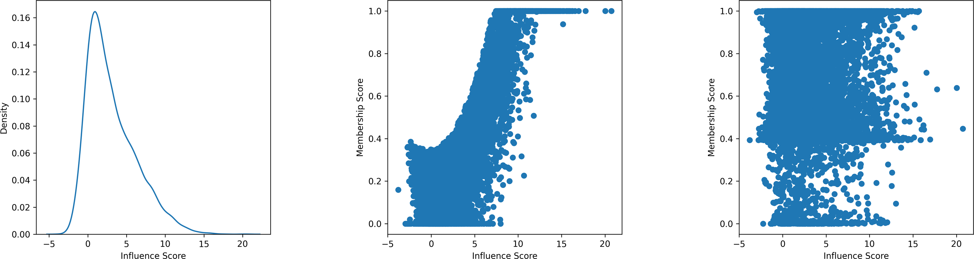
Our attack intuition. To overcome the aforementioned limitations, we propose a new attack intuition that adheres to the basic principles of difficulty calibration but improves both generality and performance. This intuition consists of two main components: aggregating membership-relevant information and inferring sample membership.
Membership information aggregation. We train each OUT model by distilling knowledge from the target model on a randomly selected subset of the auxiliary dataset. Since sample difficulty is closely related to sample membership and can be effectively quantified by the outputs of the OUT models, these outputs can be used as an indirect but informative proxy for inferring membership. The impact of knowledge distillation is twofold. On one hand, because the OUT models are optimized using a different loss function (e.g., KL divergence rather than cross-entropy), they may not fully replicate the training behavior of the target model, which could introduce output bias. On the other hand, inspired by Liu et al. (2022), we argue that membership-related signals embedded in the target model can be effectively transferred to the OUT models via distillation. Moreover, knowledge distillation uses KL divergence between the output distributions of the target and OUT models as its objective, which eliminates the need for ground-truth labels and simplifies the training process. Overall, knowledge distillation achieves a practical trade-off between fidelity and feasibility in OUT model construction.
Membership inference via neural network. Instead of using hypothesis testing as in LiRA, we propose training a neural network, referred to as the inference model, to directly predict whether a sample is a member of the target model. This inference model learns a mapping from membership-related signals (e.g., outputs of OUT models and the target model) to a predicted membership score. It is worth noting that employing neural networks in this context is a heuristic strategy. The underlying intuition is that, compared to hypothesis testing, neural networks, with their high capacity and large number of parameters, can better approximate complex mappings and thereby recognize a broader set of member samples. Specifically, we hypothesize that the inference model is capable of identifying low self-influence members that LiRA often fail to detect. This hypothesis is empirically supported by the right subplot of Fig. 1, which shows that the membership scores produced by the inference model do not exhibit a strong correlation with self-influence, indicating improved detection performance for such hard cases. A key challenge, however, lies in constructing a reliable training set for the inference model, as the adversary does not know the ground-truth labels for the target model. To overcome this, we introduce a reference model that mirrors the structure and training distribution of the target model. Using this reference model and multiple OUT models distilled from it, we obtain training samples with known membership labels (i.e., whether a sample was used to train the reference model). This enables supervised training of the inference model. While training the inference model requires additional OUT models, we mitigate the overhead by halving the number of OUT models used per attack stage, thus keeping the overall model budget constant. Subsequent experimental results also show that even with half the number of OUT models, the performance of attacks using the inference model still outperforms the performance of attacks using hypothesis testing.
Summary. Our proposed strategy distills membership-relevant signals from the target model and leverages a learned inference model to more accurately predict membership. As detailed in the ‘Ablation Study’ section, we compare the effectiveness of label-supervised models, knowledge-distilled models, hypothesis testing, and inference models to assess their individual contributions to attack performance.
Attack method
In this article, we propose a new membership inference attack, DSMIM-MIA, which targets the challenge of identifying low self-influence samples while adhering to the principle of difficulty calibration. The detailed architecture of the attack pipeline is shown in Fig. 2. Our DSMIM-MIA mainly consists of three modules: shadow model training, inference model training and inference model prediction. To prevent data leakage between modules, we randomly divide the auxiliary dataset DAux into two disjoint halves: one serving as the reference dataset DRef and the other as the shadow dataset DSha.
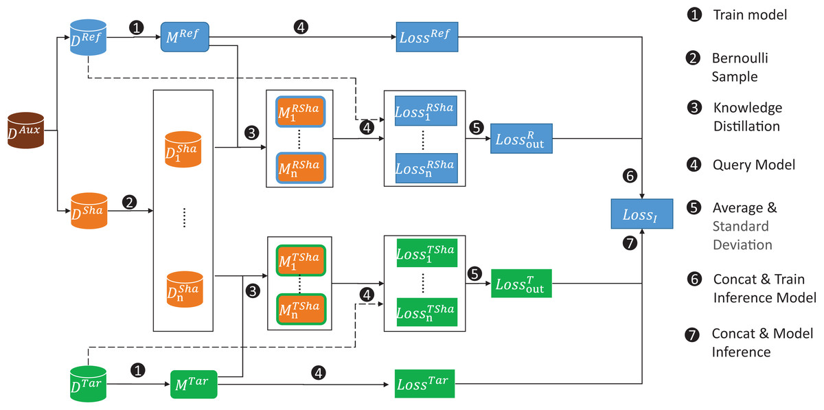
Figure 2: Our general attack pipeline for DSMIM-MIA.
First, we train the reference model with the reference dataset and the target model has already been trained. Second, we construct shadow dataset subsets using Bernoulli sampling. Third, for each subset we train the shadow model with knowledge distillation on the reference model or the target model. Fourth, we query the reference dataset for the reference model and its shadow models to obtain the original and shadow predictive losses, respectively, and do the same for the target dataset. Fifth, we take the mean and standard deviation of multiple shadow model prediction losses for each sample as the sample predictive loss features on the OUT model. Sixth, we use the concatenation of the OUT model predictive loss features and the original predictive loss as data features, the membership of the samples on the reference model as labels to form the inference model training set, and train the inference model. Finally, we obtain the data features of the target samples using similar concatenating methods and use the trained inference model to predict the membership of the target samples.
____________________________
Algorithm 1 Inference Model Training Algorithm._____________________________________________________________
Input: Reference Dataset DRef, Training Algorithm τ, Shadow Dataset DSha, Knowledge Distil-
     lation Algorithm κ, Shadow Model Numbers n
Output: Trained Inference Model I
 1:  Split DRef into two equal-sized and mutually disjoint part DRef
train and DRef
test
  2:  Mref ← τ(DRef
train)
  3:  Dinf
train ←{}
 4:  for i = 1 to n do
 5:       Bernoulli sampling DSha yields the subset DShai
  6:       MRshai ← κ(
 Mref,DShai)
 7:  end for
 8:  for each sample (x,y) in DRef do
 9:       lossRout = {}
10:       if ((x,y) ∈ DRef
train) then
11:            sign ← 1
12:       else
13:            sign ← 0
14:       end if
15:       for i = 1 to n do
16:            lossRshai ← MRshai (x)
17:            lossRout ← lossRout ∪{
 lossRshai}
18:       end for
19:       lossref ← Mref(x)
20:       μout ← mean(lossRout)
21:       σout ← std(lossRout)
22:       Dinf
train ← Dinf
train ∪{
 (lossref,μout,σout,sign)}
23:  end for
24:  I ← τ (
 Dinf
train)_________________________________________________
Shadow model training. Our attack begins with the shadow model training, which aims to obtain a set of OUT models for each sample. A shadow model is defined as a model trained on data drawn from the same distribution as the target model’s training set and sharing the same architecture. When a shadow model is queried with samples not included in its own training set, it functions as an OUT model for those samples. The shadow model training module involves two main steps: constructing the training set and setting the loss function. As shown in Fig. 2, our attack performs n times Bernoulli sampling on the shadow dataset DSha to generate training subsets . Unlike previous approaches that train shadow models with cross-entropy loss, our attack adopts the KL divergence loss between the target model ’s outputs and those of shadow models. After completing the above steps, we obtain a set of shadow models .
Inference model training. After constructing the shadow models, the next phase involves training the inference model to predict sample membership based on model outputs. This step directly addresses the challenge of accurately identifying low self-influence samples, which traditional hypothesis-based methods often fail to detect. The complete steps of the inference model training module are described in Algorithm 1 . First, we train a reference model Mref which shares the same architecture as the target model and is trained using a subset with the cross-entropy loss. Second, this module feeds each sample in the Dref to n shadow models and obtain their prediction losses . Our attack then compute the mean μout and standard deviation σout of these losses to represent the behavior of OUT models. These statistics, along with the reference model’s own predictive loss, are concatenated to form the feature representation. The membership label (indicating whether the sample was used in training Mref) serves as the ground truth. These two together form the training set of the inference model. The inference model I is then trained on this dataset using the cross-entropy loss. It is worth noting that the association between OUT model outputs and sample memberships learned by the inference model essentially only applies to the reference model. However, given the high similarity between the reference and target models, we assume that the inference model can effectively generalize to successfully predict the sample membership of the target model.
Inference model prediction. After training the inference model, the attack enters the prediction phase, where it estimates the sample membership. The procedure is detailed in the Algorithm 2 . In brief, the inference model receives two types of input features: (1) the output of the target model on the sample (2) the mean and standard deviation of outputs from shadow models. Rather than directly feeding all individual outputs from the OUT models, which may include redundant or noisy information, we use only the statistical summaries (mean and standard deviation) as feature inputs. This design reduces noise while preserving key membership-related patterns. We can formalize this as follows.
_____________________________________________________________
Algorithm 2 Inference Model Inference Algorithm_____________________________________________________________
Input: Target sample (x,y), Target Model Mtar, Shadow Dataset DSha, Knowledge Distillation
     Algorithm κ, Trained Inference Model I, Shadow Model Numbers N
Output: Target Sample Membership score p
 1:  lossTout = {}
 2:  for i = 1 to n do
 3:       Bernoulli sampling DSha yields the subset DShai
  4:       MTshai ← κ(
 Mtar,DShai)
 5:       lossTshai ← MTshai (x)
  6:       lossTout ← lossTout ∪{
 lossTshai}
 7:  end for
 8:  losstar ← Mtar(x)
  9:  μout ← mean(lossTout)
10:  σout ← std(lossTout)
11:  p ← I (losstar,μout,σout)___________________________________________________________________________________________
For any sample (x, y) in the target dataset Dtarget, our attack query the target model Mtar and the OUT models to get losstar and . Our attack then computes μout and σout over the OUT model losses, and concatenate μout, σout, and losstar into a single feature vector. The trained inference model I then uses this vector to output a membership score p. If p exceeds a predefined threshold, the sample is predicted as a member; otherwise, it is predicted as a nonmember
_________________________________________________________________________________________________________________________________
Algorithm 3 Online Inference Model Training Algorithm.____________________________________________________
Input: Reference Dataset DRef, Training Algorithm τ, Shadow Dataset DSha, Knowledge Distil-
     lation Algorithm κ, Shadow Model Numbers n
Output: Trained Inference Model I
 1:  Split DRef into two equal-sized and mutually disjoint part DRef
train and DRef
test
  2:  Mref ← τ(DRef
train)
  3:  Dinf
train ←{}
 4:  for i = 1 to n do
 5:       Bernoulli sampling DSha yields the subset DShai
  6:       Bernoulli sampling DRef yields the subset DRef
i
  7:       MRshai ← κ(
 Mref,DShai ∪ DRef
i    )
 8:  end for
 9:  for each sample (x,y) in DRef do
10:       lossRout = {}
11:       if ((x,y) ∈ DRef
train) then
12:            sign ← 1
13:       else
14:            sign ← 0
15:       end if
16:       for i = 1 to n do
17:            if ((x,y) ∈ DRef
i    ) then
18:                  lossRini ← MRshai (x)
19:                  lossRin ← lossRin ∪{
 lossRini}
20:            else
21:                  lossRouti ← MRshai (x)
22:                  lossRout ← lossRout ∪{
 lossRouti}
23:            end if
24:       end for
25:       lossref ← Mref(x)
26:       μin ← mean(lossRin)
27:       σin ← std(lossRin)
28:       μout ← mean(lossRout)
29:       σout ← std(lossRout)
30:       Dinf
train ← Dinf
train ∪{
 (lossref,μin,σin,μout,σout,sign)}
31:  end for
32:  I ← τ (
 Dinf
train)_________________________________________________
Cost and online attack. DSMIM-MIA incurs a one-time training cost. Once the inference and shadow models are trained, inference on new test samples can be performed efficiently by simply querying the existing models. This enables DSMIM-MIA to handle updated or streaming test samples with minimal computational overhead. We refer to this version as DSMIM OFFLINE. To further enhance performance, we introduce a more powerful but computationally intensive variant called DSMIM ONLINE. The full procedures for training and inference under DSMIM ONLINE are presented in Algorithm 3 and Algorithm 4 . Unlike the offline variant, DSMIM ONLINE additionally trains IN models to explicitly simulate the member case. Similar to the OUT model definition, the IN model is defined as a shadow model whose training set includes the target sample and can be referred to line 7 in Algorithm 3 and line 4 in Algorithm 4 . We believe that the comparison of the IN models’ outputs the OUT models’ outputs can drive the inference model to learn more about the sample membership. Thus, DSMIM ONLINE extends the input features of the inference model from , to , σin, μout, , and train a better inference model as shown in line 30 of Algorithm 3 . Despite its outstanding performance, DSMIM ONLINE comes with a significant runtime cost. This is mainly because DSMIM ONLINE has to spend a lot of time processing updated test samples. As shown in the Algorithm 4 , for each new test sample (x, y), all shadow models need to be retrained to fit the IN models. This makes it computationally prohibitive in settings where test samples arrive continuously or change frequently. In contrast, DSMIM OFFLINE does not require retraining because its models are fixed and independent of new inputs. In summary, DSMIM ONLINE achieves higher accuracy but at the expense of scalability, making it more suitable for static or small-scale evaluation tasks, whereas DSMIM OFFLINE is preferable for real-time or large-scale deployment.
_____________________________________________________________
Algorithm 4 Online Inference Model Inference Algorithm____________________________________________________
Input: Target sample (x,y), Target Model Mtar, Shadow Dataset DSha, Knowledge Distillation
     Algorithm κ, Trained Inference Model I, Shadow Model Numbers N
Output: Target Sample Membership score p
 1:  lossTout = {}
 2:  for i = 1 to n do
 3:       Bernoulli sampling DSha yields the subset DShai
  4:       MTini ← κ(
 Mtar,DShai ∪{x})
 5:       MTouti ← κ(
 Mtar,DShai)
 6:       lossTini ← MTini (x)
  7:       lossTouti ← MTouti (x)
  8:       lossTin ← lossTin ∪{
 lossTini}
 9:       lossTout ← lossTout ∪{
 lossTouti}
10:  end for
11:  losstar ← Mtar(x)
12:  μin ← mean(lossTin)
13:  σin ← std(lossTin)
14:  μout ← mean(lossTout)
15:  σout ← std(lossTout)
16:  p ← I (losstar,μin,σin,μout,σout)________________________________________________________________________________
Results
Experimental setup
Datasets. Our experiments focused on three datasets as follows.
(item CIFAR10 Krizhevsky, 2009). It is a benchmark dataset for image classification tasks and is widely used for MIA evaluation. It consists of 60,000 32 × 32 colour images divided into 10 classes of 6,000 images each. (item CIFAR100 Krizhevsky, 2009). It is similar to CIFAR-10, but it has 100 classes, each containing 600 images. (item CINIC10 Darlow et al., 2018). It extends CIFAR10 by adding downsampled ImageNet images to the same categories as in CIFAR10. CINIC10 also has 10 classes, but has a total of 270,000 images.
For each dataset, we set the number of samples to 10,000 for both the training and test sets of the target and reference models and extracted 20,000 samples from the remaining samples as the shadow model dataset. There is no overlap between the five sub-datasets described above, and we will vary the size of the datasets in subsequent ablation experiments to explore the performance of the attacks under different dataset distributions.
Target model architecture. To comprehensively assess the performance of the proposed attack, we conducted experiments on each dataset using multiple target model architectures, including ResNet-56 (He et al., 2016), MobileNetV2 (Sandler et al., 2018), VGG-16 (Simonyan & Zisserman, 2014), and WideResNet-32 (Zagoruyko & Komodakis, 2016). In the following experiments, the default target model architecture is ResNet-56 unless otherwise stated.
Inference model architecture. For the inference model, we used a 4-layer multilayer perceptron (MLP) with hidden dimensions [512, 128, 32], ReLU activations, and a final softmax output layer. This architecture follows the design proposed in Liu et al. (2022), where a similar architecture was shown to achieve strong performance even on low-dimensional inputs. In our ablation study, we compared this model against simpler alternatives, including a 2-layer MLP, logistic regression, and decision trees. The 4-layer MLP achieved the best overall performance across most evaluation metrics.
Metrics. We use the following evaluation metrics.
-
Log-scale ROC Curve. Receiver operating characteristic curves (ROC) are widely used to compare the true positive rate (TPR) and true positive rate (FPR) of attacks at all possible decision thresholds.
-
TPR at low FPR. The TPR at a low FPR metric evaluates the effectiveness of an attack under strict false positive constraints, such as [email protected]% FPR or TPR@1% FPR. It enables quick and intuitive comparisons between different attack configurations. However, in practice, the target FPR may not be included in the computed sequence consisting of <FPR, TPR > pairs. For instance, the evaluation may require the TPR at 0.1% FPR, while available data points only include TPRs at 0.01% and 0.12% FPR. To address this, we estimate the TPR at the target FPR via linear interpolation between the two nearest FPR points that bracket the target value (one immediately below and one immediately above the target FPR). This interpolation yields a stable and reproducible estimate of TPR at a given FPR.
-
Area under the curve (AUC) is an average-case metric widely used in many MIAs to measure the overall performance of classifiers for binary classification tasks.
Attack baselines. We mainly compare our attack (DSMIM ONLINE and DSMIM OFFLINE) with four representative MIA attacks as baselines. LIRA attack is the current SOTA attack that achieves the highest TPR at lower FPR metrics than other methods. LIRA attacks are further divided into LIRA ONLINE (Carlini et al., 2022) and LIRA OFFLINE (Carlini et al., 2022). The former is only applicable to the case of a fixed test sample while the latter can flexibly cope with an uncertain number of test samples, similar to the difference between our DSMIM ONLINE and DSMIM OFFLINE. GLIRA attack (Galichin et al., 2024) is a variant of the LIRA OFFLINE attack which performs knowledge distillation of the target model to obtain shadow models. GLIRA differs from our attack because it uses hypothesis testing to predict membership, whereas our attack uses the inference model. LOSS TRAJECTORY (Liu et al., 2022) exploits the performance discrepancy between member and nonmember samples on distilled models to reason about sample membership.
For the sake of brevity, LON, LOFF, DON, DOFF, GL, and LT are abbreviations for the above attacks LIRA ONLINE, LIRA OFFLINE, DSMIM ONLINE, DSMIM OFFLINE, GLIRA, and LOSS TRAJECTORY, respectively.
For the fairness of the comparison, the number of shadow models for each attack is equal and not greater than thirty two, and the number of data enhancements is equal and not greater than eight. LT is an exception to this rule because it requires only one shadow model to be trained and more shadow models do not improve its performance. In addition, all attacks perform data augmentation on the test samples. Since data augmentation is a common technique used in model training, the target model may have remembered the augmented sample. We randomly flip or crop the image of each sample for data augmentation and fix the number of augmented samples to eight.
Attack performance comparison
We trained twelve different target models on three datasets four model structures. Six different attacks were executed on each target model and the results are shown in Fig. 3. It is clear that for most target models, DON has the highest ROC curve height, LON the second highest, DOFF the third highest, and the other three attacks (LOFF, GL, and LT) have much lower curve heights. Since the height of the ROC curve reflects the attack’s ability to correctly identify members, the above phenomenon shows that the three attacks, LON, DON, and DOFF, are far more effective than the others. A simple explanation is that the first three attacks all employ the difficulty calibration technique while the last three do not. Another interesting point is that as the number of target model structure parameters increases (from ResNet-56 to WideResNet-32), the performance of the last three attacks improves but still falls short of the first three. This seems to indicate the impact of model structure on attack performance, which we discuss further in the ‘Ablation Study’.
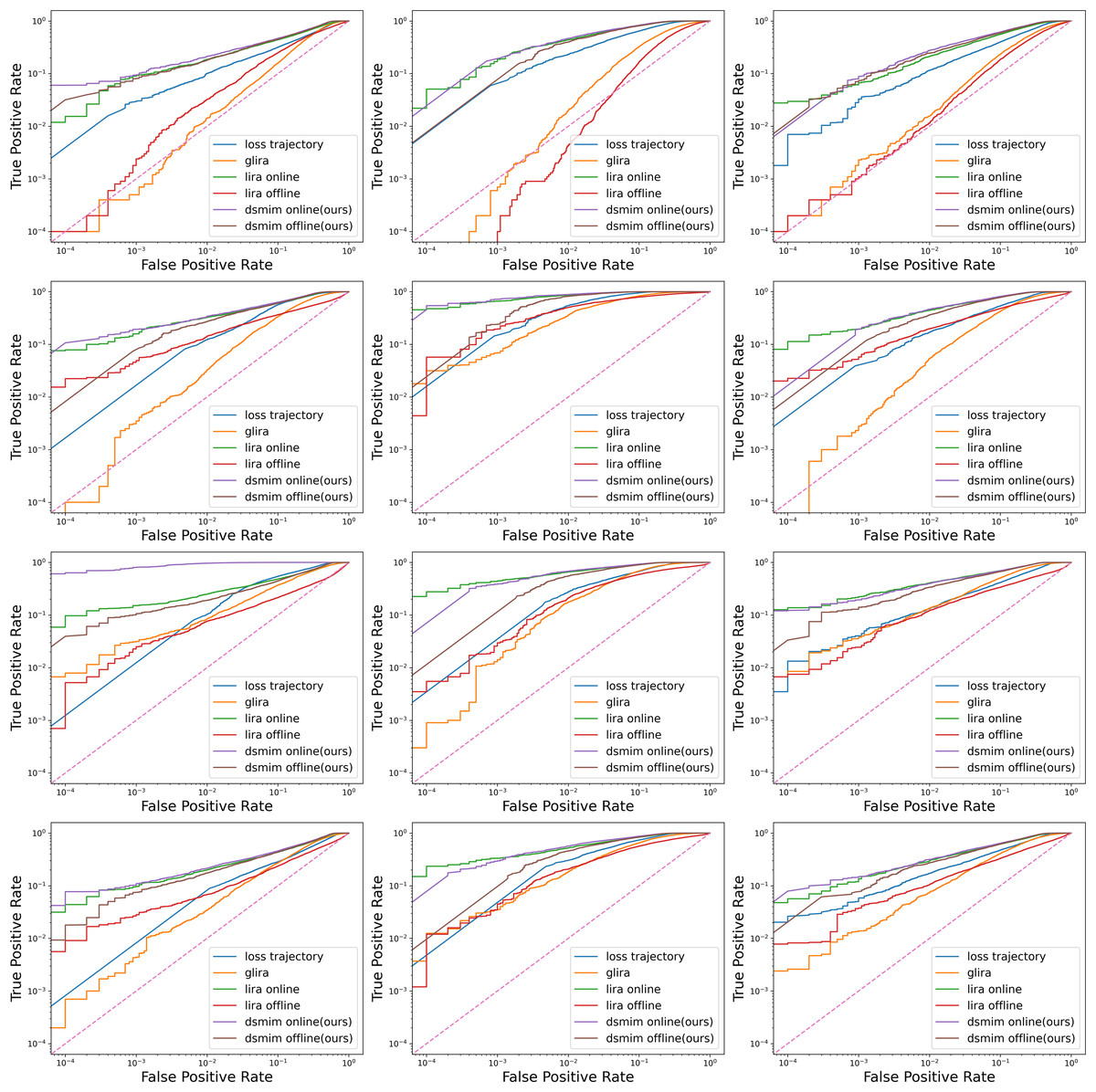
Figure 3: Log-scale ROC curves for six attacks on three datasets and four model architectures.
Dataset from left to right: CIFAR10, CIFAR100, CINIC10. Model structure from top to bottom: ResNet-56, MobileNetV2, VGG-16, and WideResNet-32.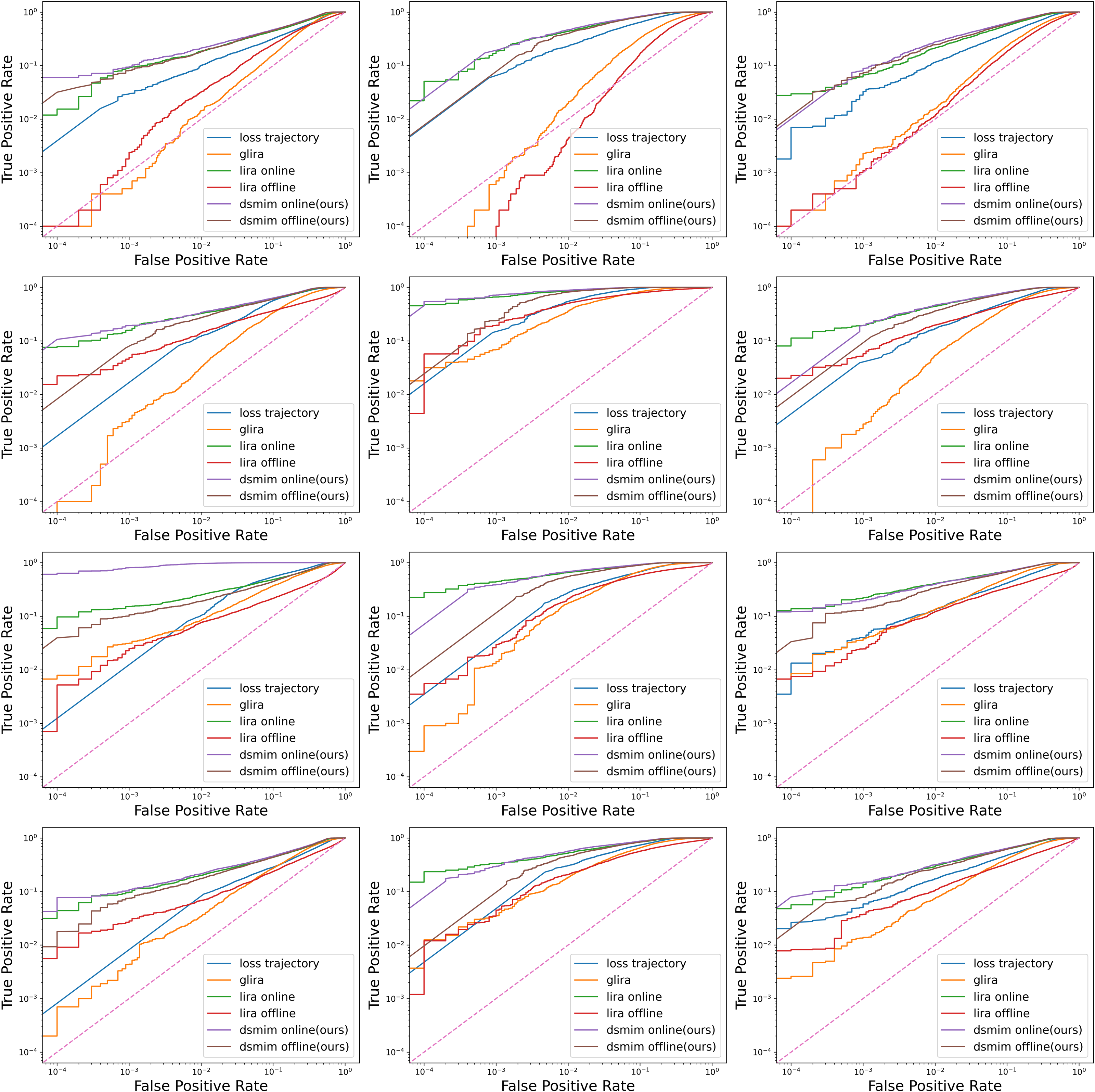
Table 1 gives the more detailed metrics of different attacks under the ResNet-56 model. Overall, the data in the table matches the curves in Fig. 3, with the three attack metrics of DON, DOFF, and LON attacks being much higher than the other three attacks. Specifically, DON attack outperforms the LON attack in all metrics, especially on the CINIC10 dataset where the metrics are higher by 2.7%, 6.7% and 2.8%, respectively. This suggests that the DON identifies more members at low error rates and is a more powerful membership inference attack than LON.
| Attack method | [email protected]%FPR | TPR@1%FPR | AUC | ||||||
|---|---|---|---|---|---|---|---|---|---|
| CIFAR10 | CIFAR100 | CINIC10 | CIFAR10 | CIFAR100 | CINIC10 | CIFAR10 | CIFAR100 | CINIC10 | |
| LT | 3.0% ± 0.53% | 5.9% ± 1.89% | 3.3% ± 1.02% | 10.1% ± 0.76% | 23.2% ± 2.89% | 11.5% ± 1.23% | 0.727 | 0.902 | 0.796 |
| GL | 0.1% ± 0.05% | 0.6% ± 0.12% | 0.2% ± 0.07% | 1.4% ± 0.27% | 2.0% ± 0.32% | 1.5% ± 0.41% | 0.689 | 0.768 | 0.694 |
| LON | 7.9% ± 1.14% | 18.7% ± 2.12% | 7.8% ± 1.25% | 19.2% ± 0.89% | 44.2% ± 3.20% | 23.1% ± 2.18% | 0.801 | 0.950 | 0.875 |
| LOFF | 0.2% ± 0.05% | 0% ± 0.00% | 0.1% ± 0.04% | 3.1% ± 0.43% | 0.4% ± 0.10% | 1.1% ± 0.33% | 0.661 | 0.679 | 0.645 |
| DON | 9.1% ± 0.93% | 20.4%± 2.29% | 10.8%± 1.30% | 20.4% ± 0.67% | 49.7% ± 2.91% | 27.6% ± 1.67% | 0.822 | 0.959 | 0.895 |
| DOFF | 7.5% ± 0.67% | 11.1% ± 1.78% | 8.4% ± 1.47% | 19.4% ± 1.31% | 40.7% ± 2.23% | 24.8% ± 1.01% | 0.818 | 0.950 | 0.890 |
In addition, the attack performance of DOFF cannot be ignored. The DOFF is slightly inferior to the LON attack in the [email protected]% FPR and TPR@1% FPR metrics, but the reverse is true in the AUC metrics. According to the metrics definition, a low TPR at low FPR represents more false identifications for member samples, while a high AUC represents less false identifications for all samples. Therefore, we believe that DOFF is slightly less capable of identifying members and slightly more capable of identifying nonmembers than LON.
Last but not least, DOFF is greater than the remaining three attacks (LOFF, GL and LT) on all metrics. This implies that our DOFF attack is the state of the art among all the attacks in the case of uncertainty in the size of the test set. Based on the above experimental results, it is clear that all three attacks, LON, DON and DOFF, perform much better than the other attacks when the number of shadow models is fixed. Therefore, our subsequent experiments focus on the comparison between these three attacks.
Attack performance with fewer shadow models
In this subsection, we compared the attacks’ performance with fewer shadow models. We conducted further experiments against the above three attacks with fewer shadow models and the results are shown in Table 2. Specifically, the TPR @1%FPR metrics of LON declined by 7.7%, 17.2%, and 10.3% on the three datasets, respectively. For the same metrics, DON decreased by 6.8%, 16.0%, and 10.9%, and DOFF decreased by 6.4%, 13.8%, and 9.2%. The above results show that the performance of the DON and LON attacks decreases rapidly and the performance of the DOFF attack decreases slowly as the number of shadow models decreases. This means that the DOFF attack will be more powerful than other attacks in some tasks where resources are severely constrained. A reasonable guess is that the shadow models for LON and DON need to fit both the IN model and the OUT model, whereas the shadow model for DOFF only needs to fit the OUT model. Thus, as the number of shadow models decreases, the quality of the LON and DON fits decreases more rapidly than the DOFF.
| Attack method | [email protected]%FPR | TPR@1%FPR | AUC | ||||||
|---|---|---|---|---|---|---|---|---|---|
| CIFAR10 | CIFAR100 | CINIC10 | CIFAR10 | CIFAR100 | CINIC10 | CIFAR10 | CIFAR100 | CINIC10 | |
| LON(shadow_num=32) | 7.9% ± 1.14% | 18.7% ± 2.12% | 7.8% ± 1.25% | 19.2% ± 0.89% | 44.2% ± 3.20% | 23.1% ± 2.18% | 0.801 | 0.950 | 0.875 |
| LON(shadow_num=16) | 6.8% ± 1.29% | 17.4% ± 3.16% | 6.1% ± 1.54% | 17.2% ± 0.50% | 40.6% ± 2.81% | 20.8% ± 1.53% | 0.788 | 0.942 | 0.862 |
| LON(shadow_num=8) | 4.7% ± 0.33% | 12.3% ± 2.11% | 4.8% ± 0.66% | 14.7% ± 0.67% | 34.1% ± 2.97% | 16.8% ± 1.36% | 0.767 | 0.927 | 0.840 |
| LON(shadow_num=4) | 3.3% ± 0.50% | 9.8% ± 1.92% | 3.3% ± 0.58% | 11.5% ± 0.63% | 27.0% ± 2.75% | 12.8% ± 0.88% | 0.737 | 0.904 | 0.806 |
| DON(shadow_num=32) | 9.1% ± 0.93% | 20.4% ± 2.29% | 10.8% ± 1.30% | 20.4% ± 0.67% | 49.7% ± 2.91% | 27.6% ± 1.67% | 0.822 | 0.959 | 0.895 |
| DON(shadow_num=16) | 7.1% ± 0.82% | 18.7% ± 1.01% | 8.9% ± 0.94% | 17.9% ± 1.02% | 44.8% ± 1.96% | 24.2% ± 1.36% | 0.807 | 0.951 | 0.883 |
| DON(shadow_num=8) | 5.8% ± 0.58% | 16.0% ± 0.97% | 8.0% ± 0.64% | 16.1% ± 0.85% | 39.0% ± 1.71% | 20.8% ± 1.04% | 0.787 | 0.940 | 0.864 |
| DON(shadow_num=4) | 5.1% ± 0.42% | 13.1% ± 1.30% | 5.4% ± 0.45% | 13.6% ± 0.86% | 33.7% ± 0.97% | 16.9% ± 0.60% | 0.764 | 0.926 | 0.840 |
| DOFF(shadow_num=32) | 7.5% ± 0.67% | 11.1% ± 1.78% | 8.4% ± 1.47% | 19.4% ± 1.31% | 40.7% ± 2.23% | 24.8% ± 1.01% | 0.818 | 0.950 | 0.890 |
| DOFF(shadow_num=16) | 6.1% ± 0.51% | 10.9% ± 1.65% | 7.1% ± 1.24% | 16.9% ± 0.99% | 36.1% ± 1.84% | 21.2% ± 1.10% | 0.802 | 0.941 | 0.874 |
| DOFF(shadow_num=8) | 4.4% ± 0.61% | 9.2% ± 1.14% | 4.9% ± 1.16% | 13.4% ± 0.90% | 28.9% ± 2.15% | 16.4% ± 0.95% | 0.776 | 0.926 | 0.850 |
| DOFF(shadow_num=4) | 4.0% ± 0.45% | 8.9% ± 0.50% | 4.5% ± 0.67% | 13.0% ± 0.44% | 26.9% ± 1.80% | 15.6% ± 0.42% | 0.744 | 0.901 | 0.814 |
Data augmentation analysis
In addition to the quantity of shadow models, data augmentation may also affect the attack performance. We varied the number of augmented samples and executed the attacks separately and the results are shown in Table 3. As the number of data augmentations is reduced from 8 to 1, the TPR @1%FPR metrics of LON on three datasets decrease by 7.3%, 12.0%, and 9.5%, respectively. For the same metric, DON decreased by 5.7%, 11.6%, and 7.2%, while DOFF decreased by 3.6%, 6.5%, and 4.4%. Therefore, we can reason that all attack performance decreases with the number of augmented samples, especially for DOFF. A simple interpretation of the above results is that the model is trained not only to minimise the loss of the original training samples, but also to minimise the loss of the augmented version of the samples (Carlini et al., 2022). More augmented samples means a closer approximation to the actual model minimum loss, and also means less error in fitting the output distribution.
| Attack method | [email protected]%FPR | TPR@1%FPR | AUC | ||||||
|---|---|---|---|---|---|---|---|---|---|
| CIFAR10 | CIFAR100 | CINIC10 | CIFAR10 | CIFAR100 | CINIC10 | CIFAR10 | CIFAR100 | CINIC10 | |
| LON(augment_num=8) | 7.9% ± 1.14% | 18.7% ± 2.12% | 7.8% ± 1.25% | 19.2% ± 0.89% | 44.2% ± 3.20% | 23.1% ± 2.18% | 0.801 | 0.950 | 0.875 |
| LON(augment_num=4) | 7.1% ± 1.29% | 17.3% ± 2.60% | 6.8% ± 1.04% | 18.0% ± 0.67% | 41.4% ± 2.42% | 21.7% ± 1.82% | 0.793 | 0.946 | 0.867 |
| LON(augment_num=2) | 5.2% ± 1.16% | 15.9% ± 2.57% | 4.9% ± 0.83% | 15.3% ± 0.53% | 37.6% ± 1.16% | 17.4% ± 0.60% | 0.781 | 0.940 | 0.853 |
| LON(augment_num=1) | 3.8% ± 0.76% | 11.0% ± 1.69% | 3.3% ± 0.59% | 11.9% ± 0.59% | 32.2% ± 1.49% | 13.6% ± 1.09% | 0.763 | 0.929 | 0.834 |
| DON(augment_num=8) | 9.1% ± 0.93% | 20.4% ± 2.29% | 10.8% ± 1.30% | 20.4% ± 0.67% | 49.7% ± 2.91% | 27.6% ± 1.67% | 0.822 | 0.959 | 0.895 |
| DON(augment_num=4) | 7.7% ± 0.88% | 20.0% ± 1.84% | 9.3% ± 0.76% | 19.3% ± 1.02% | 47.2% ± 2.29% | 25.9% ± 1.55% | 0.818 | 0.956 | 0.892 |
| DON(augment_num=2) | 6.2% ± 0.63% | 17.8% ± 2.19% | 7.9% ± 1.01% | 17.0% ± 0.74% | 43.1% ± 1.89% | 23.4% ± 1.05% | 0.814 | 0.951 | 0.886 |
| DON(augment_num=1) | 5.1% ± 0.58% | 11.8% ± 1.74% | 6.2% ± 1.18% | 14.7% ± 1.08% | 38.1% ± 2.13% | 20.4% ± 0.76% | 0.806 | 0.944 | 0.878 |
| DOFF(augment_num=8) | 7.5% ± 0.67% | 11.1% ± 1.78% | 8.4% ± 1.47% | 19.4% ± 1.31% | 40.7% ± 2.23% | 24.8% ± 1.01% | 0.818 | 0.950 | 0.890 |
| DOFF(augment_num=4) | 8.0% ± 0.73% | 10.0% ± 1.57% | 7.8% ± 1.39% | 18.6% ± 1.16% | 38.5% ± 1.92% | 24.1% ± 1.03% | 0.816 | 0.948 | 0.888 |
| DOFF(augment_num=2) | 7.8% ± 0.85% | 10.0% ± 2.30% | 7.4% ± 1.36% | 18.1% ± 0.71% | 36.3% ± 2.08% | 22.1% ± 1.31% | 0.813 | 0.945 | 0.884 |
| DOFF(augment_num=1) | 6.1% ± 0.74% | 9.9% ± 1.45% | 7.0% ± 1.78% | 15.8% ± 1.10% | 34.2% ± 1.92% | 20.4% ± 1.28% | 0.809 | 0.941 | 0.880 |
Ablation Study
In this section, we analyze the contributions of individual components to the effectiveness of DSMIM-MIA. Specifically, we examine the separate impacts of knowledge distillation and the inference model. Furthermore, we evaluate three additional factors: (1) the degree of model overfitting, (2) the target model architecture mismatch between the target and shadow models, and (3) the inference model architecture.
Individual component impact
To understand the role of each component, we compare the inference model against hypothesis testing, and knowledge distillation against label-based training. Let KD represent knowledge distillation, LT represent label training, HT represent hypothesis testing, and IM represent the inference model. By combining these components, we construct four variants of the attack LT + HT, KD + HT, LT + IM, KD + IM.
We evaluate these combinations on the CIFAR10 dataset and results are presented in the Table 4. Interestingly, we observe that knowledge distillation has both pros and cons. On the one hand, knowledge distillation weakens the ability of the OUT model to mimic the target model’s training process due to its specialized loss function (KL divergence), as evidenced by the reduced performance of KD + HT compared to LT + HT. On the other hand, knowledge distillation transfers part of the information related to membership from the target model and enhances the correlation between the OUT model’s output and membership, which can be confirmed by the superior performance of KD + IM compared LT + IM. Overall, the advantages of knowledge distillation outweigh its drawbacks, because the performance of KD + IM is better than that of LT + HT.
| Attack combination | [email protected]%FPR | TPR@1%FPR | AUC |
|---|---|---|---|
| LT+HT | 7.9% ± 1.14% | 19.2% ± 0.89% | 0.801 |
| KD+HT | 7.7% ± 1.01% | 18.1% ± 0.84% | 0.649 |
| LT+IM | 8.0% ± 0.91% | 19.8% ± 0.78% | 0.810 |
| KD+IM | 9.1% ± 0.93% | 20.4% ± 0.67% | 0.822 |
Furthermore, we observe that the inference model consistently improves all evaluation metrics, regardless of whether it is trained on ground-truth labels or distilled outputs. To better understand this improvement, we analyze the distribution of membership scores produced by the hypothesis testing method and the inference model, as shown in Fig. 4. Specifically, 98.5% of member samples evaluated by the inference model obtain membership scores greater than 0.6, whereas 31.1% of members evaluated via hypothesis testing fall below this threshold. This observation aligns with our design intuition: the inference model outperforms the hypothesis test in identifying low self-influence members due to the inference model’s stronger representational capability. In addition, while the inference model does improve the membership scores of some nonmember samples, the proportion of nonmembers in the very-high-score regions decreases compared to members. This shift in distribution provides an explanation for the inference model’s superior performance as measured by the TPR at low FPR metric.
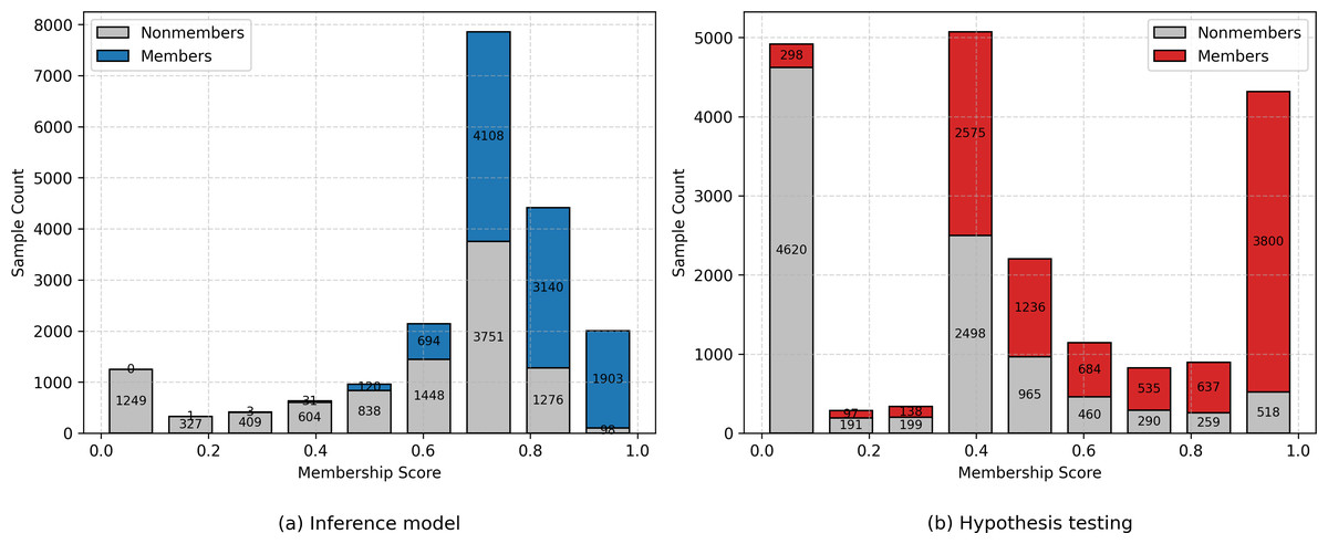
Figure 4: Histogram of membership scores for different methods on the CIFAR-10 dataset.
Each bin shows the count of member and nonmember samples separately. (A) Inference Model (Neural Network). (B) Hypothesis Testing.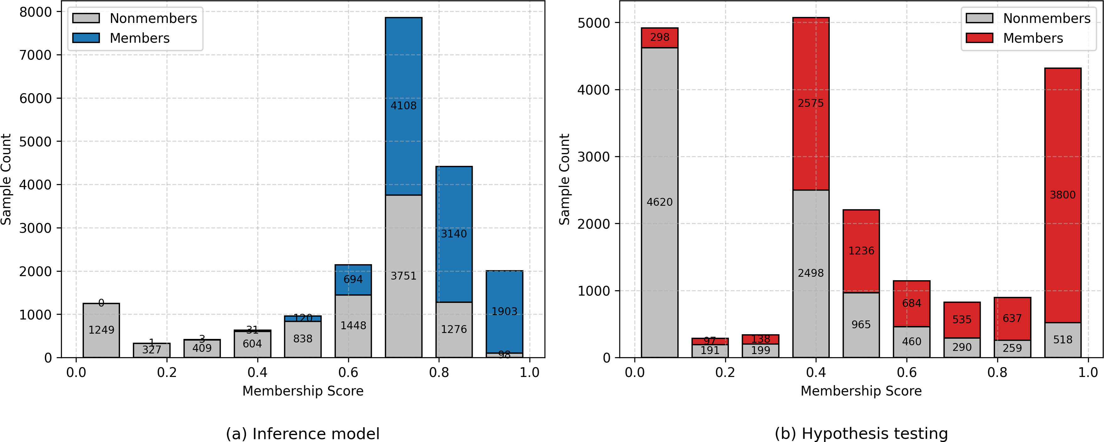
Training size impact
In the above experiments, we fixed the size of the training set for each model for comparative fairness. In this section, we will resize the training set and test the performance of DON and DOF attacks.
To obtain more training set samples, we adopt the CINIC10 dataset as the evaluation dataset, which has 270,000 images and is sufficient to support experiments with many training set samples. Here, we fix the model architecture WideResNet-32 and vary the number of training samples for the target model, keeping the same number of training samples for the target model, the reference model, and the shadow model.
As shown in Tables 5 and 6, as the training size of the target model increases, the train-test-gap of the model gradually decreases, weakening the attack’s ability to distinguish between members and nonmembers as a whole (AUC metrics decrease). However, the TPR at a low FPR metric remains relatively high with decreasing model overfitting. Under a training size of 40,000 and a well-trained target model, the DON attack achieves a 12.2% [email protected]%FPR metric, and the DOF attack achieves an 8.6% [email protected]%FPR metric. This high metric indicates that our attack can identify many membership samples at low error rates, even in well-trained models, and can be applied to models with different levels of overfitting.
| Training size | Train test gap | [email protected]%FPR | TPR@1%FPR | AUC |
|---|---|---|---|---|
| 10,000 | 0.355 | 8.9% ± 0.77% | 27.8% ± 1.35% | 0.891 |
| 15,000 | 0.301 | 13.6% ± 1.23% | 30.5% ± 1.61% | 0.879 |
| 25,000 | 0.240 | 14.1% ± 1.08% | 26.1% ± 1.04% | 0.854 |
| 40,000 | 0.205 | 12.2% ± 0.89% | 21.7% ± 1.28% | 0.811 |
| Training size | Train test gap | [email protected]%FPR | TPR@1%FPR | AUC |
|---|---|---|---|---|
| 10,000 | 0.355 | 8.4% ± 1.64% | 27.0% ± 0.94% | 0.892 |
| 15,000 | 0.301 | 12.2% ± 1.48% | 26.9% ± 1.47% | 0.873 |
| 25,000 | 0.240 | 10.5% ± 1.72% | 24.7% ± 0.87% | 0.850 |
| 40,000 | 0.205 | 8.6% ± 1.35% | 20.7% ± 1.23% | 0.811 |
Target model architecture impact
In previous experiments, we assumed the adversary knew the target model structure and aligned the reference and shadow model architectures with the target model architecture. However, the adversary may have difficulty knowing the target model structure in a real-world environment. Thus, similar to Liu et al. (2022), Carlini et al. (2022), we change the architecture of the target model, the reference model, and the shadow model while keeping the architecture of the reference model and the shadow model aligned since both models are entirely under the control of the adversary locally.
As shown in Fig. 5, our attack performs best when the target and shadow model structures are aligned. Furthermore, when the target model structure is similar to the shadow model structure (e.g., ResNet-56 and WideResnet-32), the performance of our attack is similar to that under the same structure for both. Regarding target and shadow models with entirely different structures, our attack also performs well if the shadow model size is much larger than the target model (e.g., WideResnet-32 vs. MobileNetV2). In contrast, if the shadow model size is much smaller than the target model, the performance of our attack becomes relatively worse. One possible reason is that larger models may have more complex structures and can fit smaller ones with different structures, while the reverse is untrue.
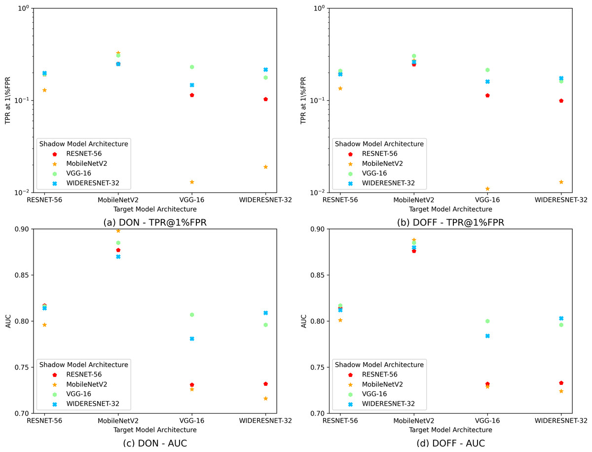
Figure 5: Impact of structural differences between target and shadow models trained on the CIFAR10 dataset.
(A) Hows the values of TPR@1%FPR on the CIFAR-10 dataset for the DISTILL ONLINE (DON) attack under varying choices of target and reference model structures. (B) Shows the values of TPR@1%FPR on the CIFAR-10 dataset for the DISTILL OFFLINE (DOFF) attack under varying choices of target and reference model structures. (C) Shows the AUC values on the CIFAR-10 dataset for the DON attack under varying choices of target and reference model structures. (D) Shows the AUC values on the CIFAR-10 dataset for the DOFF attack under varying choices of target and reference model structures. Together, (A–D) Illustrate how varying the structural choices of the target and reference models influences the performance of DON and DOFF attacks, across both TPR@1%FPR and AUC metrics.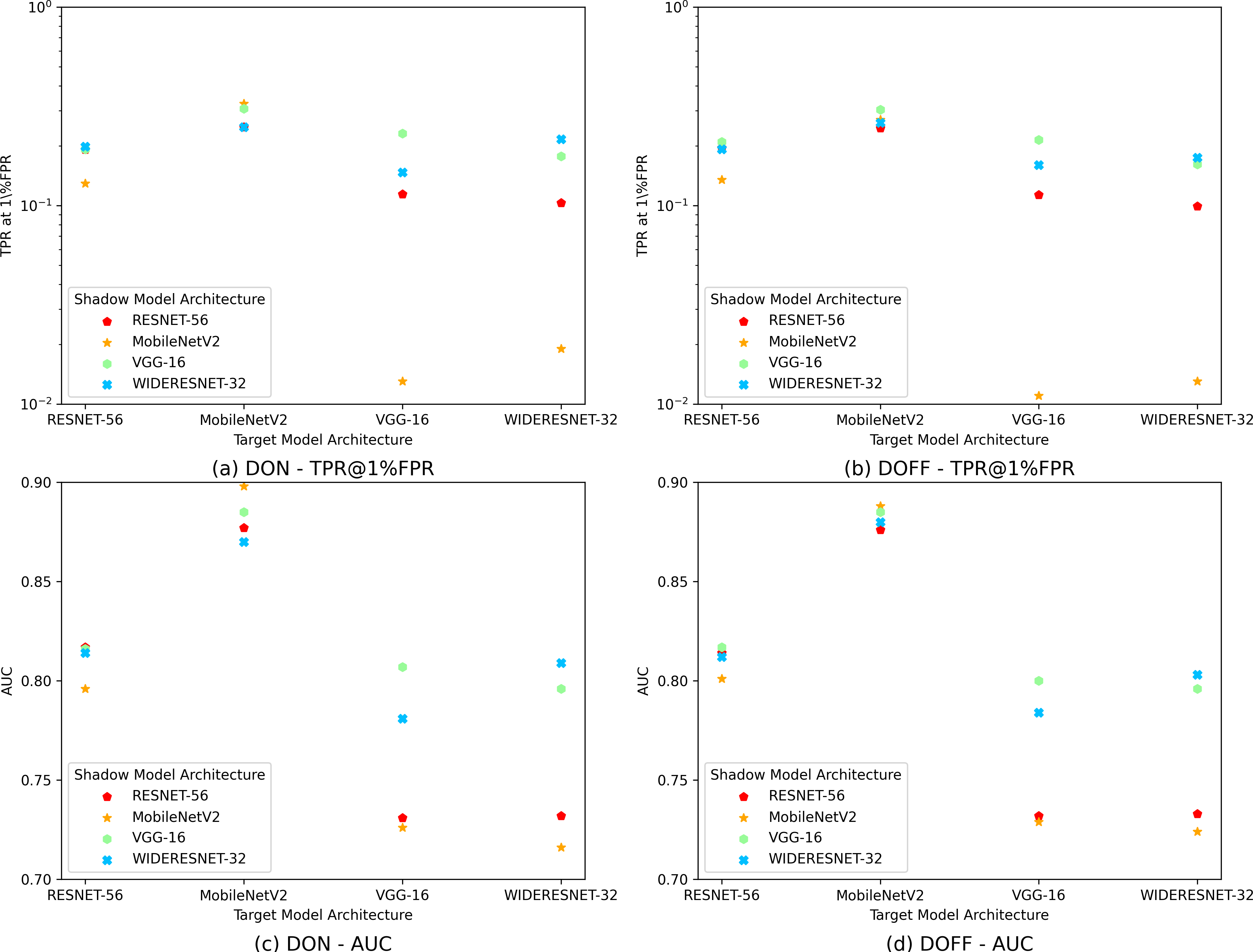
Inference model architecture impact
In our previous experiments, we employed a 4-layer MLP as an inference model. However, since the input features consist of only a few low-dimensional statistics, it is unclear whether such a complex model is necessary to capture the decision boundary effectively. To further assess the impact of model complexity, we organized three additional experiments with simpler inference model architectures: a 2-layer MLP with 32 hidden units, logistic regression, and the decision tree. We denote the 4-layer MLP as MLP4, the 2-layer MLP as MLP2, logistic regression as LR, and the decision tree as DT. Both the DSMIM ONLINE and DSMIM OFFLINE algorithms were executed with each of these inference models. Since DSMIM ONLINE uses five statistics as input features, we denote this setting as dim = 5, whereas DSMIM OFFLINE uses three statistics as input features, denoted as dim = 3.
| Attack method | [email protected]%FPR | TPR@1%FPR | AUC | ||||||
|---|---|---|---|---|---|---|---|---|---|
| CIFAR10 | CIFAR100 | CINIC10 | CIFAR10 | CIFAR100 | CINIC10 | CIFAR10 | CIFAR100 | CINIC10 | |
| MLP4(dim=5) | 9.1% ± 0.93% | 20.4% ± 2.29% | 10.8% ± 1.30% | 20.4% ± 0.67% | 49.7% ± 2.91% | 27.6% ± 1.67% | 0.822 | 0.959 | 0.895 |
| MLP2(dim=5) | 9.3% ± 0.42% | 23.2% ± 2.41% | 10.6% ± 1.04% | 19.9% ± 0.76% | 49.1% ± 2.02% | 27.1% ± 0.89% | 0.819 | 0.958 | 0.893 |
| LR(dim=5) | 6.7% ± 0.29% | 23.1% ± 3.21% | 10.6% ± 0.82% | 17.3% ± 0.89% | 47.8% ± 2.03% | 26.7% ± 0.74% | 0.803 | 0.956 | 0.891 |
| DT(dim=5) | 6.3% ± 0.41% | 22.4% ± 2.73% | 10.0% ± 0.80% | 16.7% ± 0.86% | 47.4% ± 2.13% | 25.6% ± 0.99% | 0.798 | 0.955 | 0.889 |
| MLP4(dim=3) | 7.5% ± 0.67% | 11.1% ± 1.78% | 8.4% ± 1.47% | 19.4% ± 1.31% | 40.7% ± 2.23% | 24.8% ± 1.01% | 0.818 | 0.950 | 0.890 |
| MLP2(dim=3) | 8.2% ± 0.38% | 12.0% ± 2.14% | 8.8% ± 0.87% | 19.2% ± 1.14% | 39.9% ± 2.10% | 24.4% ± 1.32% | 0.816 | 0.949 | 0.887 |
| LR(dim=3) | 7.2% ± 0.81% | 14.4% ± 1.02% | 9.1% ± 1.01% | 18.1% ± 0.71% | 39.2% ± 1.72% | 24.1% ± 1.46% | 0.806 | 0.948 | 0.886 |
| DT(dim=3) | 7.1% ± 0.91% | 13.4% ± 1.10% | 8.8% ± 1.03% | 17.9% ± 0.91% | 38.9% ± 1.87% | 23.6% ± 1.20% | 0.804 | 0.947 | 0.884 |
The experimental results are presented in Table 7. The MLP-based models consistently outperform the non-MLP models in both TPR@1%FPR and AUC metrics. This indicates that deep neural networks are more capable of capturing subtle nonlinear relationships among features, thereby achieving more accurate membership predictions with low error rates. Furthermore, MLPs achieve substantially higher [email protected]%FPR on CIFAR-10, comparable results on CINIC-10, and noticeably lower performance on CIFAR-100. These mixed results suggest that there is no consistent pattern linking adversary performance at very low false positive rates to model complexity. Interestingly, although MLP4 has significantly more parameters than MLP2, the performance gains are relatively modest. This implies that the benefits of increasing model capacity are constrained by the low dimensionality of the input features, thus limiting the advantages of hyperparameterization in this case.
Conclusions
In this work, we revealed a key limitation of LiRA and similar membership inference attacks: their effectiveness is biased toward samples with high self-influence, leading to degraded performance on low self-influence members. We formally and empirically demonstrated that LiRA’s membership scores are positively correlated with sample self-influence, which fundamentally restricts its generality. To address this issue, we propose a novel attack framework, DSMIM-MIA, which aggregates membership features through distilled shadow models and predicts membership by the inference model, ultimately removing the bias of low self-influence samples. The distillation process transfers membership-relevant signals from the target model to shadow models without requiring ground-truth labels, enabling more scalable shadow model training. The inference model adaptively learns the relationship between shadow model output and membership from the data, effectively overcoming the self-influence bias inherent in hypothesis testing. In addition, extensive experiments across multiple datasets and model architectures demonstrate that our DSMIM-MIA outperforms state-of-the-art attacks, particularly in identifying low self-influence members, thereby providing a more comprehensive assessment of training data privacy. In future work, we plan to explore alternative definitions of sample influence and their impact on membership inference, aiming to better understand and quantify data vulnerability in modern machine learning systems.
Supplemental Information
Implementation of four deep learning model architectures, namely ResNet-56, MobileNetV2, VGG-16, and WideResNet-32
Code Usage Guidelines.
Instruction on how to run the code
Deep learning model training algorithms.
Training algorithms for target, reference and shadow models
Our attack algorithm implementation.
Implementation of the DSMIM ONLINE attack algorithm as well as the DSMIM OFFLINE attack algorithm
Dataset preprocessing functions.
Import of training sets and construction of training sets for different models