
A hybrid CNN-GRU model with XAI-Driven interpretability using LIME and SHAP for static analysis in malware detection
- Published
- Accepted
- Received
- Academic Editor
- Vicente Alarcon-Aquino
- Subject Areas
- Algorithms and Analysis of Algorithms, Artificial Intelligence, Data Mining and Machine Learning, Security and Privacy, Neural Networks
- Keywords
- Explainable AI, Machine learning, Deep learning, Malware classification, Ensemble learning, Static analysis, XGBoost, CNN, GRU, SHAP
- Copyright
- © 2025 Vuran Sarı and Acı
- Licence
- This is an open access article distributed under the terms of the Creative Commons Attribution License, which permits unrestricted use, distribution, reproduction and adaptation in any medium and for any purpose provided that it is properly attributed. For attribution, the original author(s), title, publication source (PeerJ Computer Science) and either DOI or URL of the article must be cited.
- Cite this article
- 2025. A hybrid CNN-GRU model with XAI-Driven interpretability using LIME and SHAP for static analysis in malware detection. PeerJ Computer Science 11:e3258 https://doi.org/10.7717/peerj-cs.3258
Abstract
The increasing sophistication of evolving malware types and attack techniques has rendered traditional antivirus solutions inadequate, particularly in mitigating zero-day threats. To address this challenge, Machine Learning (ML) and Deep Learning (DL)-based approaches have been developed, demonstrating significant efficacy and high accuracy in malware classification. However, the black box nature of these models raises significant concerns in terms of transparency and interpretability. This study presents a comprehensive evaluation of Ensemble Learning and Deep Learning methods for static analysis-based malware classification, which allows joint analysis of Application Programming Interface (API) calls and Dynamic Link Library (DLL) data. In the study, a specially designed Convolutional Neural Network (CNN)-Gated Recurrent Units (GRU)-3 model is trained using a tailored dataset consisting of malicious and secure software. In order to better understand the model’s performance, feature importance analysis was performed using SHapley additive exPlanations (SHAP) and Local Interpretable Model-agnostic Explanations (LIME) Explainable Artificial Intelligence (XAI) techniques and the reliability of model decisions was increased. The proposed model was compared with DL models such as CNN, Long Short-Term Memory (LSTM), and GRU, as well as traditional ML algorithms such as Extreme Gradient Boosting (XGB), Extra Trees Classifier (ETC), K-Nearest Neighbor (KNN), and Random Forest (RF). While the traditional XGB model achieved the highest overall performance with a 99.81% accuracy rate, our proposed CNN-GRU-3 model demonstrated the best performance among all DL models, reaching a 99.37% accuracy rate. This study presents a powerful framework that provides both high accuracy in malware detection and makes the decision mechanism more transparent.
Introduction
With the rapid advancement of computer technologies, malware has become a significant threat to cybersecurity for individuals, organizations, and even entire nations. Therefore, it is imperative to detect and eliminate malware as soon as possible. Malware analysis is the process of understanding the behavior of malware or malicious code and determining the impact of malware on systems. Static analysis analyzes malware code without executing it (Gunduz, 2022; Calik Bayazit, Koray Sahingoz & Dogan, 2023). It is also called non-execution-based analysis. Static analysis focuses more on malware features (e.g., included text, system calls, external calls, and libraries). Using this approach, aspects and behaviors of malware such as Text/Strings/Patterns, Header, Application Programming Interface (API) Call Trace/Graphics, and Imported Libraries and File Formats are examined. Traditional techniques such as signature-based classification may not provide good results in finding unknown malware. To overcome this, Artificial Intelligence (AI)-based methods have been proposed (Yuan, Lu & Xue, 2016), which extract data from static analysis of malware and automatically classify malware from regular files and applications. AI offers techniques, approaches, and algorithms designed to address problems that require intelligent behavior (Albu, Precup & Teban, 2019). Machine Learning (ML) and Deep Learning (DL) are two of these techniques designed to protect against malware (Kadebu et al., 2023). Since then, ML (Ma et al., 2019) and DL techniques have been applied to various cybersecurity challenges, including multi-feature ensemble learning (Dai et al., 2019), static analysis for Android malware detection where recurrent neural networks like Bidirectional Long Short-Term Memory (BiLSTM) have shown high success rates (Calik Bayazit, Koray Sahingoz & Dogan, 2023), comprehensive cyberthreat detection (Ullah et al., 2022), and behavioral malware variant detection (Al-Hashmi et al., 2022). In all these cases, these techniques have been useful and have been used to detect unknown malware. Tree-based ensemble algorithms and other ML techniques have proven to be very useful in reducing false positive rates and improving prediction and classification (Euh et al., 2020). Additionally, DL algorithms have shown promise in malware identification (Aslan & Yilmaz, 2021). Static analysis looks at the content and features of the file before the malware is executed to determine the type and behavior of the malware and classifies it. To determine the presence of malware, ML and DL models use static analysis detection, which examines the code, API calls, bytes, Dynamic Link Library (DLLs), and other file attributes. For example, a neural network uses the file’s features as input to predict the type of virus and produces an output. When combined with static analysis, ML and DL models are fast and suitable for real-time malware detection, which is critical for immediate protection. This allows cybersecurity professionals to gain a deeper understanding of various malware types, behaviors, and spreading methods, allowing them to take necessary precautions. Another important advantage of ML and DL approaches is their ability to autonomously identify malicious activity and discover previously undetected threats without relying on predefined models. Despite the effectiveness of ML and DL-based malware detection, their black-box nature poses a major challenge in cybersecurity applications. Explainable AI (XAI) has emerged as a critical solution to address this issue by improving model transparency, interpretability, and trustworthiness. XAI techniques such as Shapley Additive Explanations (SHAP), Local Interpretable Model-agnostic Explanations (LIME), and Layer-wise Relevance Propagation (LRP) enable security experts to understand the reasoning behind a model’s decisions, making malware classification more reliable. This interpretability is particularly crucial for ensuring regulatory compliance, as cybersecurity regulations often mandate clear explanations for automated decisions, especially in security-critical industries. Moreover, integrating XAI into malware analysis fosters expert-human collaboration by allowing cybersecurity analysts to verify, refine, and improve ML-based detection systems based on explainable insights. By identifying the key features that influence model predictions—such as API call sequences, opcode patterns, or permission requests—XAI also helps in detecting adversarial attacks and evasion techniques used by sophisticated malware. Thus, the incorporation of explainability in AI-driven malware analysis not only enhances detection accuracy but also contributes to a more robust and secure cybersecurity ecosystem. Motivated by these observations, a new dataset containing three different models was used to classify malware and compare the effectiveness and reliability of the models. Model 1 uses Extreme Gradient Boosting (XGB), Random Forest (RF), Extra Trees Classifier (ETC), K-Nearest Neighbor (KNN), Convolutional Neural Network (CNN), Long Short-Term Memory (LSTM), and Gated Recurrent Units (GRU) to classify malware. Model 2 applies an ensemble approach that combines the best models through voting and stacking to improve classification accuracy. Model 3 introduces a custom CNN-GRU-3 model designed to leverage both spatial and sequential features for malware classification. The unique contributions of the research can be summarized as follows:
We introduce a novel hybrid CNN-GRU model specifically tailored for malware classification. We demonstrate its effectiveness by comparing its performance against not only standard ML and individual DL models but also against conventional ensemble techniques, thereby providing a comprehensive benchmark on our curated dataset. Using this dataset, we show how effective our proposed hybrid model is compared to standard ML and single DL models.
We present a tailored dataset containing various malware examples from real-world data. By including unseen data, the dataset can be considered as a reference for future research in malware classification. We provide a reliable evaluation of ML and DL methods with XAI analysis that increases the reliability of the assessments.
Unlike most studies that focus only on API calls or opcode sequences, this study integrates API Calls and DLLs for malware classification. When used together, it has proven to be more effective than analyzing API and DLL features alone. This approach differentiates this study by providing a more accurate view of malware behavior.
Although ensemble learning is well-known in other fields, it is rarely applied in Windows-based malware classification. This study contributes to the literature by demonstrating its effectiveness in this context.
To address the black-box nature of models, we incorporate XAI techniques such as SHAP and LIME to enhance interpretability in malware classification. This contribution ensures that model decisions are more transparent, facilitating trust, regulatory compliance, and expert validation. By identifying key features that influence classification, XAI helps cybersecurity professionals detect adversarial attacks and optimize malware detection strategies.
To guide our investigation, this study aims to answer the following research questions (RQs): RQ1: how does the performance of a hybrid CNN-GRU deep learning model compare to standalone deep learning models and traditional machine learning algorithms for static malware classification? RQ2: how effective is the joint analysis of API calls and DLL information for distinguishing between malicious and benign software? RQ3: what key features are most influential in model predictions, and can XAI techniques like SHAP and LIME provide transparent insights into the models’ decision-making processes? The remainder of this article is structured to address these questions.
The rest of the article is organized as follows: ‘Related Studies’ presents related studies, ‘Materials and Theorical Background’ highlight theoretical background and dataset, including malware classification methods and dataset pre-processing. ‘Experimental Results and Analysis’ presents experimental results and analysis. The study concludes by discussing research directions in ‘Conclusion’.
Related studies
There are many studies in the literature investigating the effectiveness of ML and DL techniques in malware classification and detection. Some of the studies on malware classification and detection and their methods summarized as follows. To position our research within the current academic landscape, we first provide a comparative summary of recent and relevant studies in malware detection. Table 1 summarizes these key works, outlining their methodologies, utilized features, datasets, and primary contributions.
| Reference | Methodology | Features used | Key result | Contribution/Notes |
|---|---|---|---|---|
| Bhat & Dutta (2021) | Opcode n-gram Freq. analysis | Opcode n-grams | 96.22% Acc. | A lightweight, NLP-inspired statistical approach, avoiding complex ML models. |
| Haq, Khan & Akhunzada (2021) | Hybrid CNN-BiLSTM | Permissions, API calls, Intents | 99.47% Acc. | A hybrid DL architecture for multi-vector and persistent malware. |
| Azeez et al. (2021) | Stacking ensemble (DL + ML) | PE Features | 100% Acc. | A sophisticated stacking framework using deep learning models as base learners. |
| Rezaei, Manavi & Hamzeh (2021) | DNN + K-Means clustering | PE Header (Raw Bytes) | 97.75% Acc. | A novel training approach where a DNN is guided by a clustering algorithm. |
| Gunduz (2022) | GVAE + LightGBM | API-Call graphs | 96.7% Acc. | Use of GVAE for feature learning from API-call graphs. |
| Kabakus (2022) | 1D-CNN | Permissions, Intents, API calls | 90% Acc. | Proposing a novel 1D-CNN architecture for automated feature extraction on 1D data. |
| Yousuf et al. (2023) | Ensemble learning (RF) | PE Features (DLL, API) | 99.5% Acc. | Comprehensive fusion of different static PE feature sets for improved performance. |
| Aslam et al. (2023) | Extra Trees + XAI | API & Permissions | 99.53% Acc. | Adding transparency to a high-performance ML model using Explainable AI (XAI). |
| Chen & Ren (2023) | XGBoost, Feature fusion | Binary & Assembly features | 99.87% Acc. | A forward stepwise selection algorithm for creating a highly efficient fused feature set. |
| Maniriho, Mahmood & Chowdhury (2023) | Hybrid CNN-BiGRU + LIME | Dynamic API calls | 99.07% Acc. | Proposing an end-to-end framework and a public benchmark dataset for dynamic API analysis. |
| Ma, Ryu & Lee (2024) | XAI “Reverse Analysis” | Multiple datasets | 94.2% Avg. | Proposing a “reverse analysis” process using XAI to trace back detection results. |
| Galli et al. (2024) | LSTM/GRU + XAI comparison | Behavioral API sequences | Comp. Analysis | The first comprehensive comparison of multiple XAI techniques for behavioral malware detection. |
| Baghirov (2025) | LightGBM + XAI (SHAP, LIME) | Android Permissions/APIs | 94% F1-score | Emphasizing the role of XAI in providing actionable insights over merely boosting accuracy. |
| Our work | Custom CNN-GRU, XGBoost + XAI | API Calls & DLLs | 99.81% Acc. | Proposal of a hybrid DL model with in-depth interpretability analysis using LIME and SHAP. |
Rezaei, Manavi & Hamzeh (2021) used K-means clustering with a deep neural network to reach an accuracy rate of 97.75%. Haq, Khan & Akhunzada (2021) used CNN and Bidirectional Long Short-Term Memory (BiLSTM) architectures to reach a high accuracy rate of 99.47%. Azeez et al. (2021) produced impressive results across various techniques in their investigation of ensemble learning for malware detection. Kabakus presented a framework in Kabakus (2022) that used a CNN model to attain 90% accuracy. Maniriho, Mahmood & Chowdhury (2023) demonstrated encouraging outcomes with their hybrid approach, which blends DL techniques and API call analysis. A fusion feature set technique was proposed by Chen & Ren (2023) that produced high classification accuracy rates above 99%. Similarly, Yousuf et al. (2023) demonstrated the power of comprehensive feature engineering by combining multiple static features from portable executable (PE) files, including DLLs and PE headers. Their work, which also heavily utilized ensemble learning techniques, achieved a 99.5% accuracy rate for Windows malware detection. A technique named CogramDroid was proposed by Bhat & Dutta (2021) and is centered on exploiting relative frequency patterns of opcode n-grams to detect Android malware. Some studies highlight the necessity of XAI in improving transparency, feature interpretability, and overall performance in malware detection models. Baghirov (2025) investigates the application of SHAP and LIME in malware classification and finds that Light Gradient Boosting Machine (LightGBM) achieves the highest F1-score of 94% while critical features such as getDeviceId and access significantly affect the classification accuracy. In a similar vein, Aslam et al. (2023) applied XAI techniques to a high-performance Extra Trees classifier, identifying the most influential API and permission-based features that contribute to the detection of Android malware, thereby adding transparency to a traditional ML model. Another study proposed by Ma, Ryu & Lee (2024) is an inverse analysis approach that uses XAI to backtrack malware detection results to their contributing parameters, and highlights the effectiveness of SHAP values in identifying key malware indicators. A different approach (Gunduz, 2022), uses Graph Variational Autoencoder (GVAE) to generate embeddings from API call graphs, and demonstrates improved malware detection accuracy by integrating GVAE reduced features with classifiers such as SVM and LightGBM. Additionally, another study proposed by Galli et al. (2024) evaluates XAI methods such as SHAP, LIME, LRP, and attention mechanisms in behavioral malware detection, comparing their effectiveness on DL models such as LSTM and GRU.
Materials and theorical background
Windows portable executable file format
A Windows operating system can manage executable code by using portable executables, which contain the information needed. The headers and sections in a PE file instruct the dynamic linker how to map the file into memory.
In the realm of malware detection, a critical focus lies in the analysis of Windows PE files, where the examination of API call sequences and Dynamic Link Libraries (DLLs) proves indispensable. Windows PE files encapsulate executable programs, and by scrutinizing the API call sequences embedded within them, researchers gain profound insights into the runtime behaviour of applications. This analysis becomes particularly crucial in detecting and thwarting malware, as malicious programs often exhibit distinctive API call patterns during execution. Investigating the interactions between Windows PE files, API call sequences, and DLLs enables a nuanced understanding of malware behavior, facilitating the development of effective detection strategies.
PE files are commonly used in static malware analysis techniques. Static analysis involves examining the features of an executable code without executing it, making it suitable for endpoint antivirus systems (Rhode, Burnap & Jones, 2018). Researchers have developed various methods to analyse PE files for malware detection. One approach is to extract distinguishing features from PE files using the structural information standardized by the Windows operating system (Shafiq et al., 2009). These features can be computed in real-time and used for classification between benign and malicious executables. Another method involves the analysing of PE header and section table information to detect packed malware (Maleki, Bateni & Rastegari, 2019). Features such as the count of suspicious sections and the frequency of function calls can be used for detection by extracting information from PE file format (Maleki, Bateni & Rastegari, 2019). A PE file also has numerous sections which contain the executable’s code and data. In this study, the following PE sections were used to obtain data within the scope of static analysis.
The .idata section: the program imports data and functions from DLLs, and this section specifies those imports.
The .edata section: the list of data and functions that PE file exports for other programs are found in this section.
The .rdata section: the file’s type, size, and location of several sorts of debug information are all saved in the file’s.rdata section, which also contains the debug directory.
Overall, static analysis of PE files for malware detection involves extracting features such as structural information, API calls, and byte/entropy histograms from PE file format. These features can be used for classification between benign and malicious executables. Various techniques, including ensemble-based (EB) and DL algorithms, have been employed for this purpose.
Dataset and data pre-processing
The executable code can be managed by the Windows operating system using portable executable files with the necessary information. The analysis of Windows PE files, especially the examination of API call sequences and DLLs, is a significant area of interest in the field of malware identification (Rhode, Burnap & Jones, 2018; Maleki, Bateni & Rastegari, 2019; Moreira, Moreira & Sales, 2024). API calls exchange data between two software components, allowing one application to send requests to the other for specific functions or data. On the other hand, DLLs contain ready-made code fragments and functions that the software needs to perform certain functions (Yousuf et al., 2023). C-Prot Cyber Security Technologies company provided the dataset for this study, which was collected from real-world environments and consists of PE files with their corresponding API calls and DLLs. The initial dataset contained a balanced collection of 1,000 malicious and 1,000 benign software samples, for a total of 2,000 samples. To create a more substantial dataset for training our deep learning models and to prevent class imbalance, we applied an upsampling technique. This process expanded the dataset to a final count of 8,000 samples, equally balanced with 4,000 malicious and 4,000 benign instances. The raw data for the initial samples can be accessed at https://c-prot.com/en/research (both benign and malware samples). A sample table of the dataset is also provided in Table 2.
| SHA-256 | Size | Digital sign. | Libraries | Functions | Label |
|---|---|---|---|---|---|
| e57d065… | 1,564,672 | 0 | WINMM.dll, comdlg32.dll, GDI32.dll, KERNEL32.dll | GetProcessId, GetSystemTime, EnumCalendarInfo, CloseClipboard, RegUnLoadKey | Malicious |
| 9372bc5b… | 59,528 | 1 | WINMM.dll, VCRUNTIME140.dll, ole32.dll | GetVersion, GetSystemTime, GetDesktopWindow, Sleep, IsDebuggerPresent | Benign |
| 4ea1879… | 41,376 | 1 | USERENV.dll, ntdll.dll, WINSTA.dll | GetService, InitOnceExecuteOnce, GetVersion, DelayLoadFailureHook | Benign |
| 815b16e… | 1,939,173 | 0 | kernel32.dll, WS232.dll, ADVAPI32.dll | SHA, ShowWindow, SetLastError, CreateProcess, VirtualProtect | Malicious |
| 7529eb8… | 80,562 | 0 | KERNEL32.dll, OLE32.dll, cygwin1.dll | GetStdHandle, GetSystemDirectory, SetDllDirectory, GetDriveType | Malicious |
| c5961d1… | 116,280 | 1 | ntdll.dll | GetSystemTime, OpenThread, ZwQueryAttributesFile | Benign |
| 4368370… | 90,448 | 0 | GDI32.dll, user32.dll, KERNEL32.dll | MapUserPhysicalPages, ReadConsoleOutputAttribute, SetConsoleScreenBufferSize | Malicious |
The initial dataset consisted of a balanced set of 2,000 samples. A data augmentation step was performed to provide more data specifically for our deep learning models. We used a simple random oversampling (upsampling with replacement) technique using Scikit-learn’s resampling function. This method involves randomly copying samples from the existing dataset until each class (benign and malignant) reaches a target size of 4,000 samples, resulting in a balanced final dataset of 8,000 samples. We chose this approach over synthetic data generation methods like synthetic minority oversampling technique (SMOTE) because our primary goal was to balance the class distribution for stable training rather than generating new, artificial data points, which can be challenging and potentially noisy for high-dimensional, sparse feature spaces like ours. To reduce the risk of overfitting associated with oversampling, we incorporated powerful regularization techniques like Dropout and Batch Normalization into our deep learning models, along with early stopping during training. Then, CountVectorizer is applied to convert the text data into a numerical form since API calls and DLLs consist of textual information. This step generates a feature matrix based on word counts by calculating the frequency of each word in each document (Goya, 2021). Thus, the frequency of each word is represented as a numerical value, making this matrix suitable for use in ML and DL algorithms. CountVectorizer is preferred instead of one-hot encoding because a large number of unique API calls and DLL names can lead to a large size explosion. Following the vectorization of textual features, which resulted in a high-dimensional and sparse feature space, we employed a two-stage dimensionality reduction strategy to create a compact, robust, and information-rich feature set. Stage 1: Feature Filtering with SelectKBest. As an initial filtering step, we used the SelectKBest method with the analysis of variance (ANOVA) F-statistic (f_classif). This univariate selection technique identifies and retains features that have the strongest individual relationship with the target variable. We chose to keep the top k = 1,000 features at this stage. This number was selected to be broad enough to include all potentially significant features while discarding the vast majority of irrelevant or noisy ones, effectively serving as a high-pass filter for feature relevance. Stage 2: Dimensionality Reduction with Principal Component Analysis (PCA). The 1,000 features selected by SelectKBest still contain significant multicollinearity. To address this, we subsequently applied PCA. PCA transforms the correlated features into a smaller set of uncorrelated variables called principal components, which preserve the maximum possible variance from the original data. The number of components was set to 300. This value was determined empirically by analyzing the cumulative explained variance, which confirmed that 300 components are sufficient to retain over 93.39% of the total variance in the 1,000-feature set. This two-stage approach is highly effective: SelectKBest first removes the statistically weakest features, and PCA then condenses the remaining features into a lower-dimensional space by eliminating redundant information. Also, it identifies the features most strongly associated with the target variable, which improves model performance and reduces computational complexity (Kilic, Essiz & Keles, 2023). This process facilitates a more efficient and faster learning process for our models by reducing computational complexity without significant information loss.
Model 1: vanilla ML and DL for malware classification
In malware classification through static analysis, ML and DL approaches are of critical importance (Gibert, Mateu & Planes, 2020). These methods make it possible to identify and classify malware at scale by automating the analysis process (Manzil & Naik, 2023). Malware analysts can decrease the time and effort needed for manual analysis by utilizing the power of ML and DL to boost the accuracy and speed of malware detection (Maniriho, Mahmood & Chowdhury, 2023). In Model 1, we compared the classification performance using four popular ML-based boosting algorithms (e.g., KNN, RF, XGB, and ET) and three popular DL algorithms (e.g., CNN, LSTM, GRU). This model serves as a reference for Models 2 and 3, and the results obtained from Model 2 and Model 3 will be compared against this baseline. Each of these classifiers is briefly described in the following paragraphs.
K-nearest neighbor
The K-Nearest Neighbor (KNN) algorithm is one of the supervised learning methods and is used in classification and regression problems. KNN uses neighboring data points to determine the class of a data point. The model uses the K nearest neighbors to determine which class a point belongs to. For a new data point, the distances to all training examples are calculated. Mathematically:
(1)
The labels of the K nearest neighbors are determined. The most frequently occurring class is assigned as the class of the new point (Eq. (2)).
(2)
K is the number of neighbors, usually represents a specific neighbor or class, and represents the class label of the neighbor selected in the KNN algorithm.
eXtreme gradient boosting
Gradient Boosting is an ensemble learning method that sequentially produces a number of weak learners, typically decision trees. Each succeeding tree fixes the errors of the preceding one, producing a robust and precise model (Friedman, 2001). Extreme Gradient Boosting (XGB) is an optimized version of the gradient boosting technique (Chen & Guestrin, 2016). It is basically a robust ensemble model that minimizes the error rate by using decision trees as weak learners. XGB builds a model by improving the estimation function step by step with the Eq. (3):
(3)
Here, is the prediction of the sample, T is the total number of decision trees, is the prediction made by the tree. XGB learns each new tree to correct the errors made by the previous model and minimizes the error function by optimizing based on the second derivative. The general loss function is defined as Eq. (4):
(4)
Here, is the loss function, is the model complexity penalty function (regularization), is the previous estimates, is the update done by the new tree. These penalty terms create smaller and more generalizable trees.
(5)
is the complexity penalty of the tree structure and is the L2 penalty applied to the leaf node weights.
Random forest
Random Forest is an ensemble learning algorithm that combines decision trees to form a strong model (Breiman, 2001). This method trains each tree on a different bootstrap sample (random subsets created by re-selecting) and uses a randomly selected subset instead of all features at each node. In this way, the similarity of the trees to each other is reduced and the risk of overfitting is reduced. In the estimation process of the model, while majority voting is used in classification problems, the average of the tree outputs is taken in regression problems. Classification is done by majority vote:
(6)
is the each decision tree, where 1 is an indicator function that counts how many trees vote for class . where is the prediction from tree , and is the number of trees.
Extra tree classifier
ETC is an ensemble learning method similar to the Random Forest algorithm but with some fundamental differences. It focuses on reducing the risk of overfitting while increasing the accuracy of tree-based models. While each decision tree in Random Forest is trained with bootstrap samples (randomly selected subsets from the dataset), Extra Trees constructs trees using the entire dataset. While Random Forest selects the best feature and the best split point to determine the best split at each node, Extra Trees selects the split points of each feature completely randomly. This randomness allows the trees to be more independent of each other and increases the generalization ability by reducing the variance of the model.
Convolutional neural network
CNN is a feed forward neural network that consists of convolutional operations and a depth structure, and is a typical algorithm for DL (Lecun, Bengio & Hinton, 2015). CNNs consist of a series of layers, such as a convolutional layer, an activation layer, a pooling layer, etc. The convolutional layer, often called the convolutional kernel, serves as the core of the neural network. In addition, the features obtained by the convolution layer are passed to the next layer, the pooling layer. Pooling layers usually act as an intermediate layer between the convolution and fully connected layers. This layer reduces the number of parameters in training and the computational cost while keeping overfitting under control (Essiz et al., 2024).
Long short-term memory
Neural networks in the Recurrent Neural Network (RNN) class are designed to process data sequentially. These networks employ recurrent connections to keep their memory of previous inputs (Graves & Schmidhuber, 2005). Because RNNs excel at tasks with temporal dependencies, they are suitable for time-series data analysis, which includes the analysis of bytecodes and API calls for malware detection. RNN processes sequences by updating its hidden state at each time step using the following equations:
(7)
(8)
Here, is the hidden state, is the input vector, and are the weight matrices, is the bias, is the activation function and is the output.
LSTM was developed to solve the problems of gradient vanishing and exploding that are frequently encountered in basic RNNs (Yalda et al., 2024). According to Hochreiter & Schmidhuber (1997), it has memory cells and switching mechanisms that improve the storage and utilization of important data across extended time periods. LSTM is powerful in capturing long-term dependencies in sequential data, making it effective for analyzing complex behavioral patterns in malware samples. Unlike LSTM, GRU is another type of RNN intended to address the vanishing gradient issue and simplify the architecture. It effectively captures long-term dependencies in sequential data because it employs migration techniques to control information flow and maintain the memory of pertinent data over time (Fu et al., 2024).
(9)
(10)
(11)
(12)
(13)
(14) where W and U present the weight matrices for each gate, and denotes the sigmoid function (Liu et al., 2024). Equations (9), (10), (11) presents , , and where are the forget state, update state, and output state gates, respectively. stands for the output vector of the previous moment, while presents the input vector. Equation (4) presents which is the hidden internal state calculated with the current input and the previous state , Eq. (13) presents the cell state and Eq. (14) presents the output vector .
Gated recurrent units
Unlike LSTM, GRU is another type of RNN intended to address the vanishing gradient issue and simplify the architecture. It effectively captures long-term dependencies in sequential data because it employs migration techniques to control information flow and maintain the memory of pertinent data across time (Fu et al., 2024). GRU uses fewer parameters to simplify the LSTM structure. Equations are as follows:
(15)
(16)
(17)
(18)
Here, as presented in Eqs. (15), (16), and are the update and reset gates, Eqs. (17), (18) present as the candidate and as the updated hidden states.
Model 2: ensemble learning for malware classification
Ensemble methods aim to achieve higher accuracy, generalization, and robustness compared to individual models (weak learners) by leveraging model diversity and error reduction to improve prediction results (Gurcan, 2025). Ensemble learning can be particularly effective in malware classification because it combines multiple models to capture complex patterns and subtle variations that a single model might miss (Euh et al., 2020; Mihalache & Burileanu, 2023). Malware data presents unique challenges, such as high dimensionality, diverse patterns across different malware families, and imbalanced class distributions (malicious vs. benign). Different models specialize in capturing different aspects. For instance, neural networks such as CNN and LSTMs excel at identifying sequential patterns in API call sequences, while tree-based methods such as RF or XGB effectively handle structured data with complex feature interactions. Combining these models allows an ensemble to leverage each model’s strength in capturing distinct characteristics of malware data. In Model 2, an ensemble framework is implemented by integrating the predictions of top-performing models through a soft voting classifier, where the probabilities generated by each model are averaged to determine the final prediction (Mim, Majadi & Mazumder, 2024).
Model 3: custom CNN-GRU-3 model for malware classification
The custom CNN-GRU-3 model is designed to classify malware based on the API Calls and DLLs. The model employs a combination of CNN and GRU networks to automate the classification of sequential feature maps for this custom malware classification task. The pseudocode for custom CNN-GRU-3 model is given in Algorithm 1. The CNN component extracts complex features, while the GRU component handles their classification. The model has three convolutional layers, three pooling layers, three GRU layers, and one fully connected layer. The size of the convolutional layer used for feature extraction is 3 × 3. We use the ELU activation function (Clevert, Unterthiner & Hochreiter, 2015). Maxpooling layers with 2 × 2 kernels reduce feature map dimensions, followed by a flattening layer that converts the output into a one-dimensional vector. The model architecture includes a GRU layer with 512, 256, 128 neurons, a depth 3, and a dropout rate of 0.3. Finally, a fully connected dense layer with 64 neurons and a Rectified Linear Unit (ReLU) activation function was added, followed by a dense layer with a single neuron and a sigmoid activation function. This GRU component improves the model’s capacity to discern intricate patterns within the sequential data. The optimization process for the model involved 150 epochs and a batch size of 64 during training. The Adam optimizer, which has a learning rate of 0.001, was preferred for its adaptive learning rate calculations, making it a suitable choice for efficient optimization. The overall design of the malware classification system used in the study is represented in Fig. 1 below.
| Inputs: Draw: Raw dataset of malware and benign samples, k: Number of top features for SelectKBest (e.g., 1,000), ncomponents: Number of principal components for PCA (e.g., 300). |
| Outputs: Mtrained: The trained classification model, Pmetrics: Performance metrics on the test set (Accuracy, F1-score, etc.). |
| — 1. Data Preprocessing — |
| 1: ▹ Upsample the dataset to 8,000 samples |
| 2: |
| 3: ▹ Convert text to a numerical matrix |
| 4: |
| 5: |
| 6: |
| 7: |
| 8: ▹ Final feature vector after dimensionality reduction |
| — 2. Model Training and Evaluation — |
| 9: |
| 10: // For Deep Learning Models (e.g., CNN-GRU-3): |
| 11: ▹ Reshape data for CNN input, e.g., to (samples, 300, 1) |
| 12: |
| 13: ▹ See function below for architecture |
| 14: |
| 15: ▹ Early-stopping is applied |
| 16: |
| 17: |
| 18; |
| 19: function Build_CNN_GRU_Model |
| 20: ▹ Input shape based on n_components from PCA |
| 21: |
| 22: |
| 23: |
| 24: |
| 25: |
| 26: ▹ Output is a sequence for GRU layers |
| 27: |
| 28: |
| 29: |
| 30: |
| 31: |
| 32: |
| 33: |
| 34: |
| 35: return model |
| 36: end function |
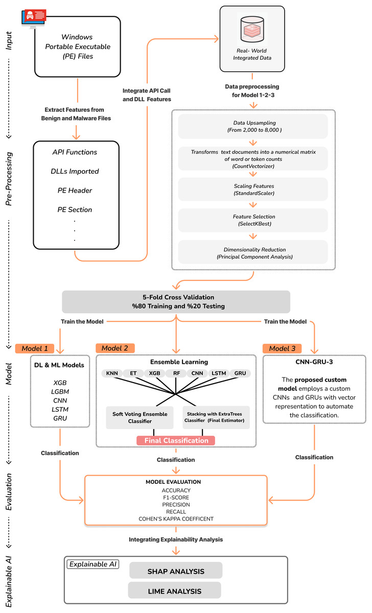
Figure 1: The overall design of the malware classification system.
The overall computational complexity of our approach, detailed in Algorithm 1, encompasses both data preprocessing and the CNN-GRU-3 model itself. The preprocessing pipeline is primarily constrained by PCA, which has a complexity of approximately , where N is the number of samples and k is the number of features before reduction. Following this, the complexity of the CNN-GRU-3 model is determined by its most demanding components. While the 1D CNN layers are efficient, the dominant factor is the stack of GRU layers. The complexity of a single GRU layer is , where T is the sequence length (300 in our case, determined by PCA components), n is the number of hidden units, and d is the feature dimension of the input to the layer. For each of the T timesteps in the input sequence, a GRU layer performs matrix multiplications between the input (dimension d) and the previous hidden state (dimension n). The operations involving the recurrent n n weight matrices are the most costly, resulting in a per-layer complexity of . As the number of hidden units (n) is a key hyperparameter and typically large, this expression is dominated by the quadratic term, simplifying to . Consequently, the model’s training complexity per epoch is largely driven by these operations. The inference complexity for a single sample, involving only a forward pass, follows the same order, ensuring that despite the intensive training, predictions remain computationally feasible for real-world applications.
Explainable artificial intelligence (XAI)
Explainable AI (XAI) is an approach that aims to make the decision-making processes of artificial intelligence models transparent and understandable (Galli et al., 2024; Ma, Ryu & Lee, 2024). Although ML and DL-based systems have high success rates, especially in the field of cybersecurity, how their decisions are made is often unclear. This poses a serious problem in terms of the reliability and applicability of the models. XAI provides security analysts with more explainable results by understanding the internal processes of the model through techniques such as LIME (Ribeiro, Singh & Guestrin, 2016), SHAP (Lundberg & Lee, 2017), LRP (Bach et al., 2015), and the attention mechanism (Bahdanau, Cho & Bengio, 2015). Understanding the reasons behind the decisions made by autonomous models provides a more reliable system (Qamar & Bawany, 2023). In the field of malware detection, AI techniques have been widely adopted due to the inadequacy of traditional signature-based methods. In particular, static and behavioral analysis methods are used to detect malware. However, the fact that these models are generally “black box” makes it difficult for security analysts to understand which features the model classifies a software as malicious (Aslam et al., 2023). At this point, XAI techniques play an important role in making malware analysis more transparent and determining the basic attributes that affect the decisions of the models (Baghirov, 2025). For example, by using SHAP values, the most effective API calls and permissions in the model’s decisions can be determined, while with the help of LIME, it can be explained on a local basis which inputs the model made a certain classification. As a result, XAI not only increases model accuracy in malware detection, but also contributes to the development of more reliable and interpretable artificial intelligence systems in the field of cybersecurity.
SHapley additive exPlanations
SHAP (SHapley Additive Explanations) (Lundberg & Lee, 2017) is a game theory-based approach to explain the predictions of a ML model. It mathematically determines how much weight the model gives to which features and how each input contributes to the prediction. SHAP is based on the concept of Shapley values (Shapley, 1953). Shapley values are a method used in game theory to fairly measure the contribution of each player to the game. SHAP adapts this approach to ML models and calculates the contribution of each feature to the model’s prediction. SHAP measures the positive or negative impact of features on the prediction by calculating the contribution of each feature on the model’s prediction. For example, the Shapley value represents the contribution of the API call in the sequence to the prediction. It increases transparency by explaining the decisions made by the model.
Local interpretable model-agnostic explanations
LIME (Local Interpretable Model-agnostic Explanations) is a model-agnostic method developed to explain the predictions of complex and unexplainable (black-box) models at a local level (Ribeiro, Singh & Guestrin, 2016). The basic assumption of LIME is that although a model has a complex decision function in general, this function can be approximated by a linear model around a specific sample (local region). LIME applies the following steps to explain a specific data sample predicted by a model: (i) Data Perturbation: it creates a neighborhood set ( ) by randomly generating perturbed data points around the targeted sample (S). For example, in a malware analysis model, LIME creates different variations by changing certain parts of an API call sequence. (ii) Generating Predictions with a Black-box Model: the newly created data points are fed to the analyzed black-box model (e.g., a CNN or LSTM model) and its predictions are obtained. (iii) Training a Weighted Linear Model: a local linear model ( ) is trained using the model’s predictions on these corrupted examples. The target function used here is defined by the following optimization problem:
(19)
is the error (unfaithfulness) between the Black-box model and the local model created, and is a regularization term that limits the complexity of the local model (Galli et al., 2024). (iv) Extraction of Feature Importances: LIME analyzes which features are weighted by the linear model created and explains the decision mechanism of the model. In malware analysis, LIME can be used to understand why a particular set of API calls is classified as malicious or safe. For example, it can show that a model detects malware based on API calls such as ‘NtCreateFile’ and ‘RegOpenKey’.
In malware classification, the output of the model (e.g., probability of malware) is taken and assigned to neurons in the last layer as an importance score R. The importance score received by each neuron is distributed to neurons in the previous layer. Importance is backpropagated using weighting rules. As a result, it is calculated how much each input feature (e.g., API calls or opcode sequences) contributes to the model prediction.
Experimental results and analysis
This study applies ML and DL on a real-world dataset for malware classification through static analysis, with Google Colab PRO+ for high-performance processing, and uses Keras 2.10.0, Scikit-learn 1.5.2, and TensorFlow 2.10.0 as the back end to build, train, and evaluate DL models (Google, 2024; Keras, 2024; TensorFlow, 2024). In this study, hyperparameter optimization was performed with the Grid Search method to ensure the best performance of the models. The hyperparameter configurations for all evaluated models are provided in Table 3.
| Algorithm | Hyperparameter | Value |
|---|---|---|
| RF | n_estimators | 100 |
| max_depth | 3 | |
| min_samples_split | 2 | |
| min_samples_leaf | 2 | |
| XGB | n_estimators | 100 |
| max_depth | 10 | |
| learning_rate | 0.1 | |
| KNN | n_neighbors | 7 |
| weights | Distance | |
| distance_metric | Euclidean | |
| ETC | n_estimators | 50 |
| max_depth | 20 | |
| min_samples_split | 2 | |
| min_samples_leaf | 1 | |
| CNN, GRU, LSTM (Baseline) |
Activation | ReLU, Sigmoid |
| Dropout | 0.3, 0.4 | |
| Learning rate | 0.0001 | |
| Batch size | 32 | |
| Epochs | 150 | |
| Optimizer | Adam | |
| CNN-GRU-3 (Proposed) |
CNN Layers | 3 (64 filters each) |
| GRU Layers | 3 (256, 128, 64 units) | |
| CNN kernel size | 3 | |
| Pool Size | 2 | |
| Activation | ELU, ReLU | |
| Dropout | 0.3, 0.4 | |
| Learning rate | 0.0001 | |
| Batch size | 64 | |
| Optimizer | Adam |
The evaluation of the models was conducted as follows: first, the entire upsampled dataset of 8,000 samples was split into a training set (80%, 6,400 samples) and a final, held-out test set (20%, 1,600 samples). For the traditional Machine Learning models (XGBoost, RF, KNN, etc.), we performed hyperparameter optimization using the GridSearchCV utility. This process involved a five-fold cross-validation scheme applied only on the training set to find the optimal combination of hyperparameters for each model. Subsequently, the model with the best-found parameters was retrained on the entire training set and its final performance was evaluated on the single, held-out test set. For the Deep Learning models (CNN, LSTM, GRU, and CNN-GRU-3), the models were trained directly on the training set, and their performance was similarly evaluated on the same held-out test set. The baseline DL models (CNN, GRU, LSTM) were structured with three layers and a varying number of units (32, 64, 128), regularized with dropout rates of 0.3 and 0.4. These models were trained for 150 epochs with a batch size of 32 and a learning rate of 0.0001, utilizing ReLU and sigmoid activation functions. For our proposed CNN-GRU model, the optimized hyperparameters, including a batch size of 64 and the Adam optimizer with a 0.0001 learning rate, are also listed in Table 3.
Evaluation metrics
Evaluating the model is one of the essential aspects of the assessment methodology (Tharwat, 2022). Performance metrics include accuracy, precision, recall, F1-score and Cohen’s kappa coefficient ( ). The confusion matrix is a framework for assessing the performance of any classifier, and it consists of four numbers: True Positive (TP): represents the number of samples correctly classified as malicious. True Negative (TN): represents the number of correctly classified benign samples. False Positive (FP): represents the number of samples incorrectly classified as malicious. False Negative (FN): represents the number of samples incorrectly classified as benign. The accuracy determines how many malicious and benign samples are correctly classified. Evaluates the effectiveness of the algorithm by calculating the ratio of the actual value of the class label (Sokolova, Japkowicz & Szpakowicz, 2006). Accuracy is calculated as follows:
(20)
Recall determines the rate of correctly classified malicious samples to all malicious samples. Recall is calculated as follows:
(21)
Precision determines the rate of correctly classified malicious samples to all malicious predicted samples. Precision is calculated as follows:
(22)
The F1-score is a harmonic mean of precision and recall for a more precise evaluation of the model performance. The F1-score is a composite metric that evaluates algorithms with greater sensitivity and tests those with greater specificity. F1-score is calculated as follows:
(23)
Cohen’s kappa coefficient, denoted as , is a statistical measure used to assess the level of agreement between two raters or classifiers beyond that which would be expected by chance. It is calculated as:
(24)
represents the observed agreement between the raters or classifiers. represents the expected agreement between the raters or classifiers by chance. indicates perfect agreement between the raters or classifiers. indicates agreement equivalent to that expected by chance. indicates agreement worse than expected by chance.
Results of ML and DL models
This section addresses RQ1 and RQ2 by presenting a comparative performance analysis of the evaluated models. Table 4 compares the accuracy, F1-score, precision, recall and Cohen’s kappa values of ML and DL models. The highest accuracy (99.81%) was obtained by the XGB model and it also exhibited a strong performance with the highest F1-score (99.81%) and 100% recall. Among the traditional ML algorithms, KNN, RF and ETC models show a strong performance with accuracy values ranging from 99.62% to 99.75%. Among the DL models, CNN stands out with 99.25% accuracy, while LSTM (98.87%) and GRU (96.31%) have lower accuracies. Custom CNN-GRU combination performed better than the stand-alone DL models by providing 99.37% accuracy.
| Model | Accuracy (%) | F1-score (%) | Precision (%) | Recall (%) | Cohen’s kappa (%) | Training time (s) | |
|---|---|---|---|---|---|---|---|
| PCA (Ours) | XGB | 99.81 | 99.81 | 99.62 | 100.00 | 99.62 | 0.55 |
| KNN | 99.68 | 99.68 | 99.62 | 99.75 | 99.37 | 0.07 | |
| ETC | 99.62 | 99.62 | 99.62 | 99.62 | 99.24 | 0.57 | |
| RF | 99.75 | 99.75 | 99.62 | 99.87 | 99.49 | 4.62 | |
| CNN | 99.25 | 99.25 | 99.25 | 99.25 | 98.50 | 47.57 | |
| LSTM | 98.87 | 98.88 | 98.15 | 99.62 | 97.74 | 1,186.26 | |
| GRU | 96.31 | 96.34 | 95.80 | 96.88 | 92.62 | 1,196.96 | |
| CNN-GRU-3 | 99.37 | 99.37 | 99.37 | 99.37 | 98.74 | 5,410.91 | |
| Stacking | 99.18 | 99.17 | 98.86 | 99.49 | 98.37 | 1,078.36 | |
| Voting | 99.25 | 99.23 | 98.98 | 99.49 | 98.49 | 980.72 | |
| Without PCA | XGB | 99.31 | 99.31 | 99.13 | 99.50 | 98.62 | 0.33 |
| KNN | 99.25 | 99.25 | 98.77 | 99.75 | 98.49 | 0.13 | |
| ETC | 99.62 | 99.62 | 99.26 | 100 | 99.24 | 0.78 | |
| RF | 99.43 | 99.44 | 98.89 | 100 | 98.87 | 1.02 | |
| CNN | 99.81 | 99.81 | 99.62 | 100 | 99.62 | 61.17 | |
| LSTM | 98.12 | 98.10 | 97.97 | 98.22 | 96.24 | 3,040.17 | |
| GRU | 95.62 | 95.57 | 95.33 | 95.81 | 91.24 | 3,155.34 | |
| CNN-GRU-3 | 95.06 | 95.12 | 94.71 | 95.53 | 90.12 | 7,542.18 | |
| Stacking | 98.11 | 97.47 | 95.97 | 99.17 | 96.03 | 2,740.32 | |
| Voting | 98.91 | 98.59 | 98.02 | 99.17 | 97.73 | 2,530.06 |
Ensemble methods such as Stacking (99.18%) and Voting (99.25%) also showed stable performance. The GRU model has the lowest Cohen’s kappa value (92.62%) and it is seen that it makes more misclassifications compared to the other models. In general, the ML-based XGB model provides the best performance, while hybrid DL models such as the proposed custom CNN-GRU also give competitive results. The quantitative impact of applying PCA is detailed in Table 4. The results present a compelling case for its inclusion in our preprocessing pipeline, revealing a critical trade-off between predictive accuracy and computational efficiency. For traditional machine learning models, particularly XGBoost, applying PCA led to a significant improvement in performance, with accuracy increasing from 99.31% to 99.81%. This suggests that PCA effectively reduced noise and collinearity in the feature set, allowing the model to identify more robust patterns. Conversely, for our deep learning models, an opposite trend was observed. The CNN model’s accuracy, for instance, dropped from a remarkable 99.81% without PCA to 99.25% with PCA. This indicates that deep learning architectures, especially CNNs, are capable of learning valuable representations directly from higher-dimensional data, and that dimensionality reduction via PCA may lead to a loss of critical information for these models. However, the most dramatic and consistent impact of PCA was on training efficiency across nearly all models. As evidenced by the training times, applying PCA led to substantial reductions in computational cost. For instance, the training time for the deep learning models was drastically lowered, with the CNN-GRU-3 model’s training duration decreasing from over 2 h (7,542.18 s) to just over 1.5 h (5,410.91 s).
The confusion matrices of ML, DL models and ensemble models are represented in the figure at https://doi.org/10.5281/zenodo.17403616. It is observed that top-performing models such as XGBoost, RF, and CNN exhibit very few misclassifications. In contrast, the GRU model shows a comparatively higher number of both false positives and false negatives, which aligns with its lower overall accuracy reported in the figure at https://doi.org/10.5281/zenodo.17403616. The proposed CNN-GRU-3 model demonstrates a more balanced error distribution, indicating a robust performance.
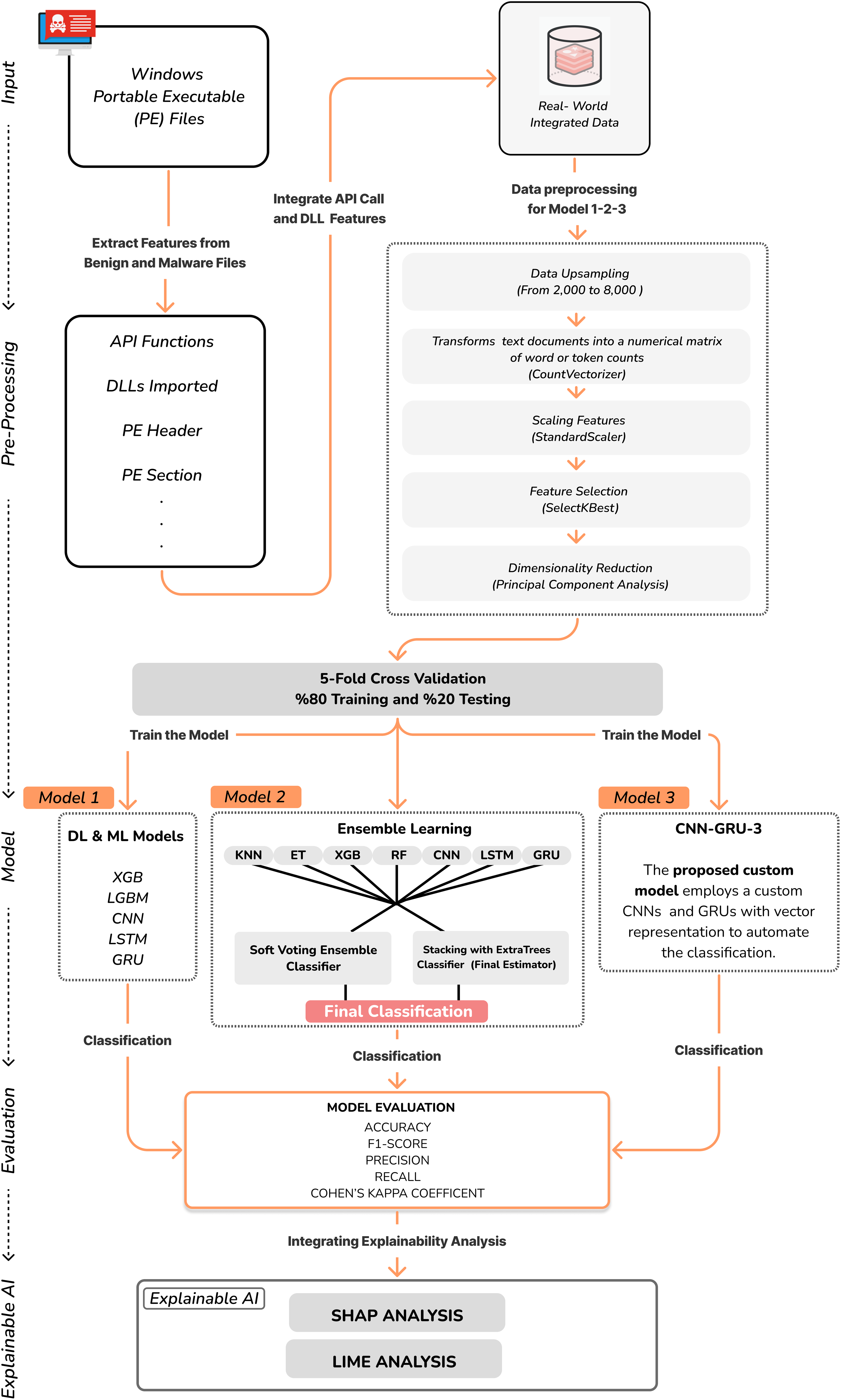
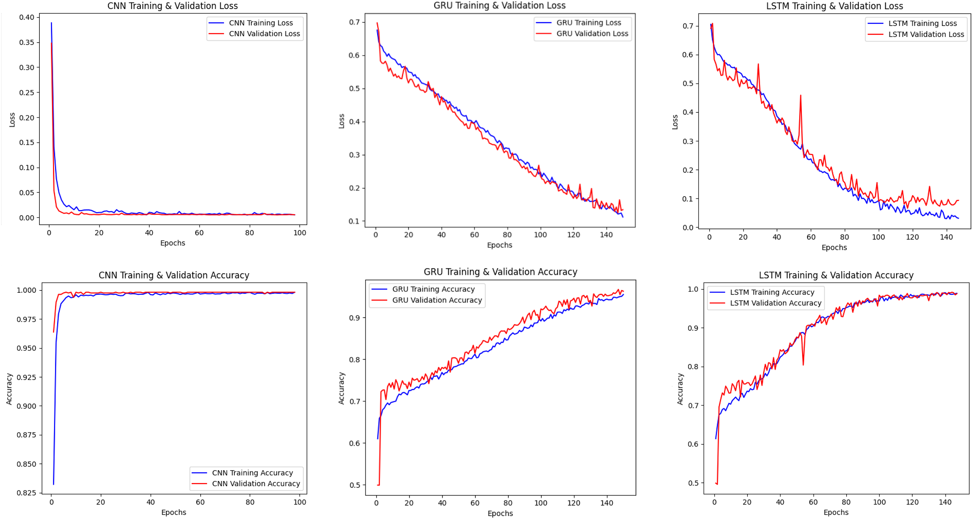
Figure 2 shows the training and validation losses and accuracies of CNN, LSTM and GRU models. The CNN model showed rapid learning in the early epochs and reached low loss and high accuracy in a short time. The LSTM and GRU models became stable in a longer time, and it was seen that the learning process was more irregular, especially in the GRU model.
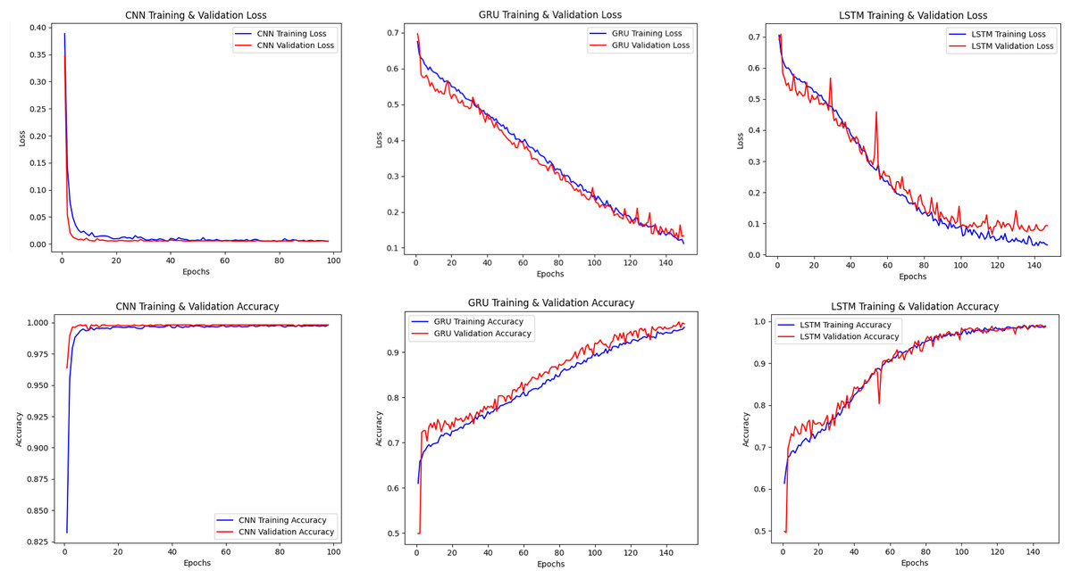
Figure 2: Accuracy-loss curves of the CNN, LSTM, GRU models.
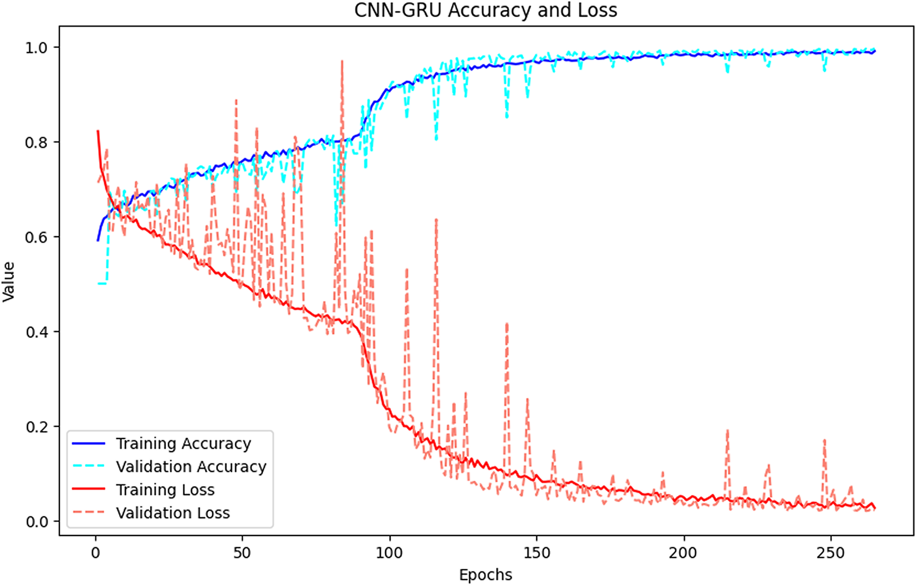
Figure 3 presents the changes in the training and validation losses of the CNN-GRU hybrid model. It was observed that the model increased its accuracy rate rapidly in the early epochs, but the validation loss became irregular after certain epochs. In particular, although the training loss decreased rapidly, the fluctuations in the validation loss indicated that the model could over-learn at certain points. However, as a result, the CNN-GRU model reached high accuracy and became one of the best performing models.
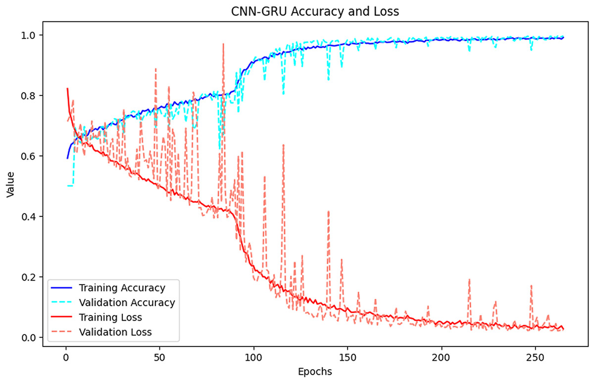
Figure 3: Accuracy-loss curves of the CNN-GRU-3 model.
While the XGB model achieved superior accuracy with a significantly shorter training time (0.55 vs. 5,410.91 s), the value of the CNN-GRU-3 model lies in its fundamentally different learning approach. As evidenced by our SHAP analysis, XGB, as a tree-based ensemble, excels at identifying and exploiting highly discriminative, individual static features. Its decisions are based on a series of splits on feature values, effectively learning a set of powerful rules (e.g., ‘if API call X is present, the probability of malware is high’). This approach is high-speed and effective when such clear indicators exist in the data. In contrast, the CNN-GRU-3 architecture is designed to understand context and sequence. The CNN layers act as pattern detectors, identifying local motifs of API calls or DLL sequences, while the subsequent GRU layers learn the long-range temporal dependencies between these patterns. Essentially, while XGB analyzes a ‘bag-of-features’, our hybrid model analyzes the grammar of the executable’s behavior. This capability is crucial for detecting more sophisticated malware that may avoid using obvious ‘red-flag’ features but exhibits malicious behavior through the specific order of its operations. While this deep architectural approach inherently leads to a substantially higher training time and computational cost, its potential for greater generalization capacity against novel or obfuscated threats presents a compelling trade-off. This investment in training is therefore justified for scenarios where detecting the nuanced grammar of malware behavior is paramount.
A notable result from our experiments is the 100% recall achieved by the XGBoost model, indicating zero false negatives. To provide a technical explanation for this perfect score beyond statistical chance, we performed a data-driven analysis of the feature distribution, focusing on the most influential features identified by SHAP. Our investigation revealed a nuanced and counterintuitive situation. A simple presence/absence analysis of top features showed that they were not simple “smoking gun” indicators of malignancy. In fact, many were paradoxically more prevalent in benign software. For instance, in our test set: the API call setunhandledexceptionfilter, despite its importance in the SHAP analysis, was present in only 31.73% of malicious samples but in a vast 88.69% of benign samples. Similarly, rtlvirtualunwind was found in just 3.44% of malicious executables compared to 75.98% of benign ones. This demonstrates that XGBoost’s perfect recall is not achieved by relying on any single deterministic feature. Instead, it is a direct result of the model’s sophisticated ability to capture complex feature interactions and non-linear relationships. As a tree-based ensemble, XGBoost learns decision paths where the predictive meaning of a feature is highly conditional on the presence or absence of others. For example, the model may have learned a highly specific rule such as: if Feature A is present AND Feature B is absent AND rtlvirtualunwind is also present, then classify as malware with high confidence. Therefore, the 100% recall is a testament to the model’s capacity to learn the subtle, combinatorial patterns within the feature space that perfectly separate the malicious class in our dataset. This highlights that the model’s strength lies in understanding the context of how features appear together, rather than just their occurrences.
In summary, the results underscore the efficacy of both advanced ensemble methods and hybrid deep learning architectures for malware classification. Our findings reveal a compelling performance landscape: the XGBoost model emerged as the top-performing model overall, demonstrating the power of gradient boosting on this type of feature-rich dataset. Simultaneously, our proposed Custom CNN-GRU-3 model distinguished itself as the most accurate among all deep learning models evaluated. This strongly suggests that its architecture, which combines spatial and sequential feature extraction, is particularly well-suited for identifying complex malware patterns. Collectively, these findings highlight that both optimized traditional methods and custom DL architectures are powerful tools for static malware analysis, providing a reliable foundation for future research.
Statistical significance analysis
To rigorously assess whether the observed performance differences between the top-performing models were statistically meaningful or merely due to chance, we conducted McNemar’s test. This test is well-suited for comparing two classifiers on the same dataset by analyzing their disagreements. We focused on key model pairs, including the overall best model (XGBoost), our proposed hybrid model (CNN-GRU-3), and other relevant benchmarks. The resulting p-values, evaluated at a significance level (alpha) of 0.05, are presented in Table 5.
| Model pair | P-value | Statistically significant? (alpha = 0.05) |
|---|---|---|
| XGBoost vs. CNN-GRU-3 | 0.0455 | Yes |
| CNN-GRU-3 vs. CNN | 0.0233 | Yes |
| XGBoost vs. CNN | 0.4795 | No |
| XGBoost vs. RF | 1.0000 | No |
| XGBoost vs. GRU | 0.0000 | Yes |
| CNN-GRU-3 vs. CNN | 0.0000 | Yes |
The results from the statistical analysis provide several critical insights. Firstly, the performance advantage of XGBoost over our proposed CNN-GRU-3 model is statistically significant . This confirms that for this specific dataset and feature set, the XGBoost model is demonstrably superior in terms of predictive accuracy. The performance difference between XGBoost and our proposed Secondly, our proposed CNN-GRU-3 model shows a statistically significant improvement over the standalone CNN model . CNN-GRU-3 model is statistically significant (p = 0.0455), confirming that XGBoost’s higher accuracy is not due to chance on this dataset. Crucially, the analysis also reveals that our CNN-GRU-3 model performs significantly better than the standalone CNN model (p = 0.0233). This provides strong evidence that the hybrid architecture, specifically the addition of GRU layers, offers a meaningful and statistically valid improvement over a standard CNN. As expected, the performance differences between models from the same family (e.g., XGBoost vs. RF) were not statistically significant. This finding is crucial as it validates our core architectural hypothesis: the integration of GRU layers to process sequential patterns provides a tangible and statistically meaningful benefit beyond what a standard CNN architecture can achieve alone. The tests also confirm the large performance gaps between the top models and the GRU model, as expected.
Explainable AI results
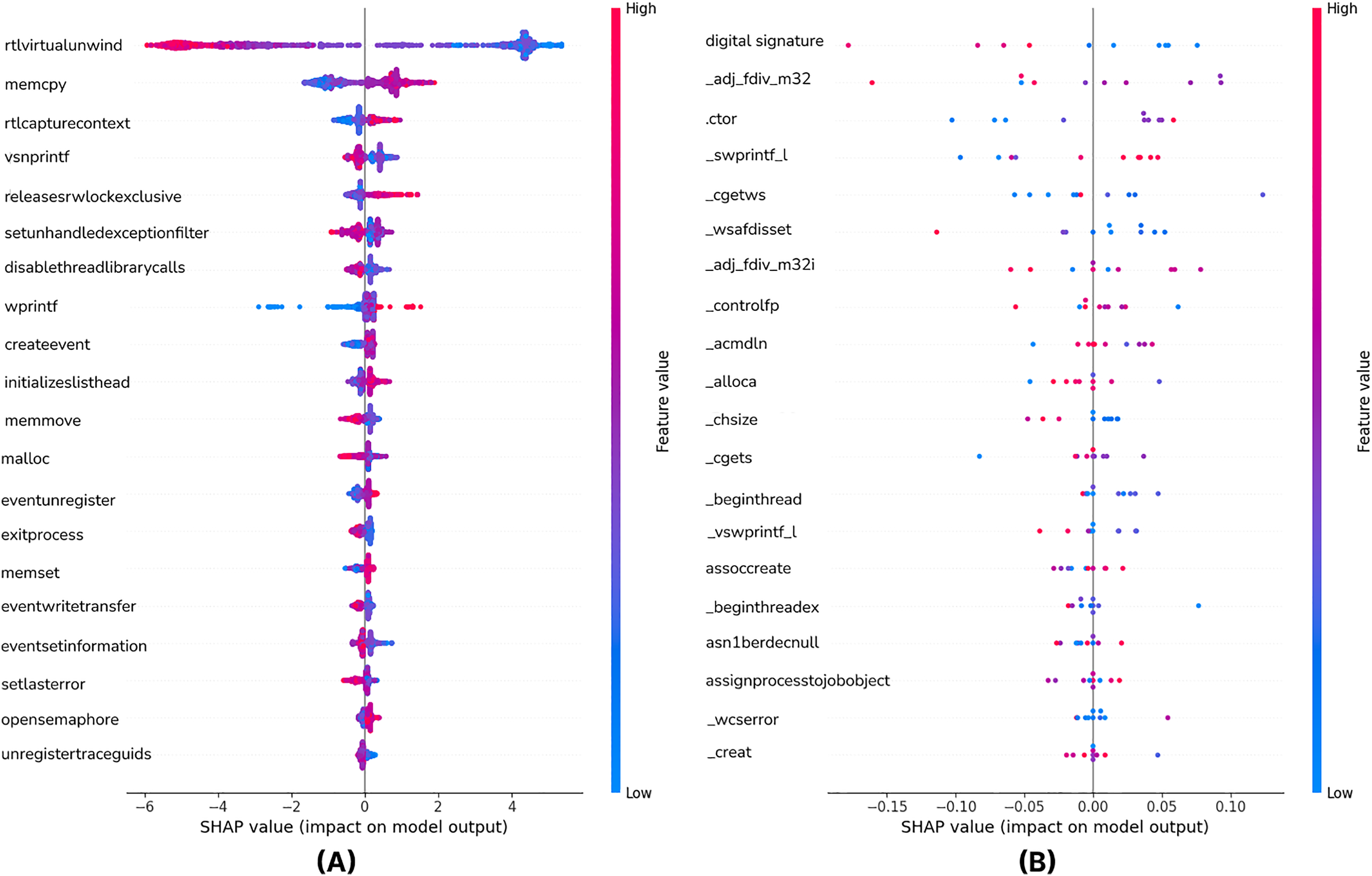
To answer RQ3, we employed XAI techniques to interpret the decisions of our best-performing models. This analysis aims to identify the most influential features and enhance the transparency of the ‘black-box’ models. Figure 4 is the SHAP Summary Plot of the XGB model showing which features affect the predictions the most on all the test data of the model. The most important features used in our model are listed. The Y-Axis (Features) lists the most important features used in the model. The X-axis is the SHAP value. It shows the effect of a feature on the model prediction. Negative values (<0) decrease the model’s prediction (for example, it pushes it more towards the benign class). Positive values (>0) increase the model’s prediction (for example, it pushes it more towards the malware class). API calls such as rtlvirtualunwind, memcpy and rtlcapturecontext are seen to be the strongest determinants in malware detection. The positive and negative SHAP values show that whether these features are specific to malware varies depending on the context. In particular, functions such as createevent and exitprocess are used in both malicious and legitimate software, so their impact varies between samples. The color scale in the SHAP graph highlights the impact of the feature values; red tones represent high values and more malware contribution, while blue tones indicate low values and generally unclear impact. These analyses show that certain API calls play a critical role in malware detection, but attackers can manipulate these calls to evade detection. Therefore, it is understood that static analysis techniques should include more adaptive and multivariate approaches.
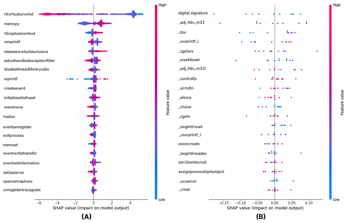
Figure 4: The shapely values of the top 20 features with the XGB (A) and CNN-GRU-3 (B) model (Summary plot).
From Fig. 4, it can be seen that features such as Digital Signature, _adj_fdiv_m32 and .ctor play an important role in the model’s prediction.
Features such as asn1berdecnull, assignprocesstojobobject, assoccreate seem to have less effect on the model. SHAP values vary between −0.15 and 0.10, meaning they have a strong but balanced effect on the model’s decisions. Some features contribute to the model’s malware prediction when they have high values (red dots are more intense at positive SHAP values), and the top 20 impactful features based on SHAP values are illustrated in the summary plot of Fig. 4.
Figure 5 is the dependence plot of the XGB model (a) shows the effect of the rtllookupfunctionentry API call on malware detection. The disablethreadlibrarycalls variable also contributes to the model as a secondary factor.

Figure 5: SHAP dependence plot of the XGB (A) and CNN-GRU-3 (B) model.
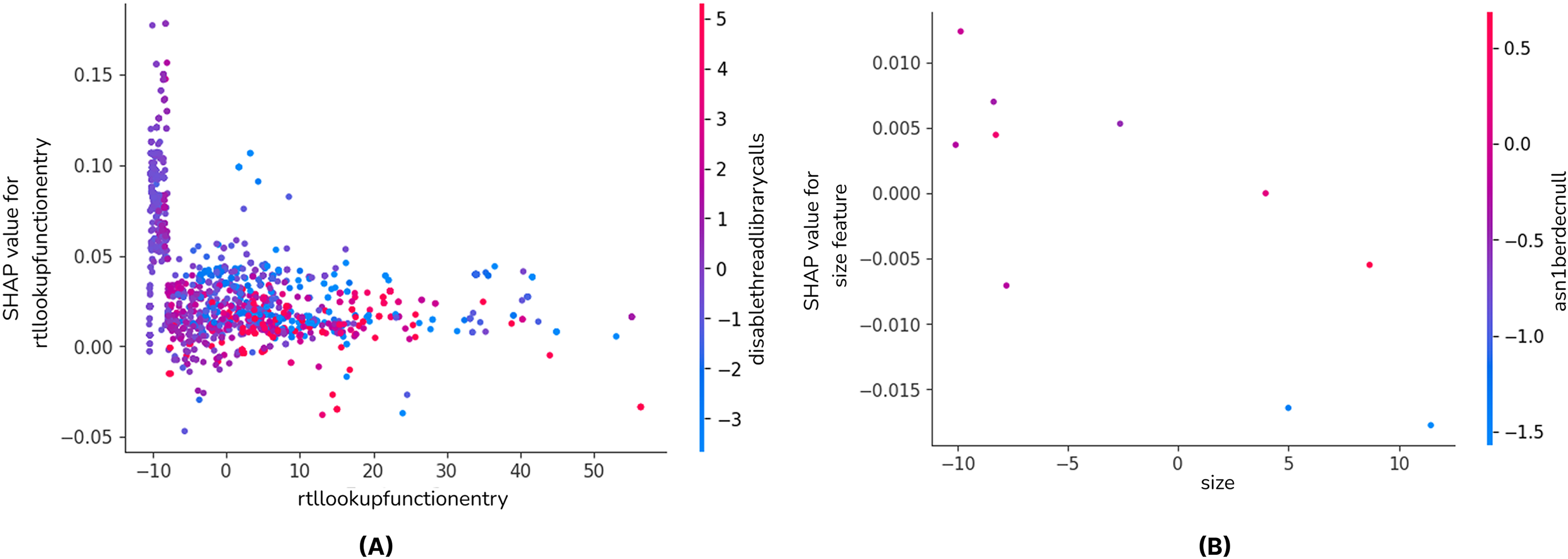
When the SHAP values are examined, it is seen that the contribution to malware detection fluctuates as the rtllookupfunctionentry values increase. The fact that the majority of the points are concentrated around zero indicates that this feature gains meaning in interaction with other API calls rather than being a sole determinant. The fact that the SHAP contribution is not significant, especially at low values, reveals that this API call affects the decision mechanism of the model only under certain conditions.
In the dependence plot of CNN-GRU-3 (b), SHAP values tend to decrease slightly as the value of size feature increases, but a very strong correlation is not observed. There is no significant change in SHAP values, especially at negative and positive values, which may indicate that this feature has a limited effect on the model’s decision. To summarize these results, when the SHAP analysis of XGBoost and CNN-GRU models is compared, the XGBoost model has a wider SHAP distribution, while the CNN-GRU model focuses more on a few important features. XGBoost evaluates all features as independent variables and calculates the effect of each on the model output. On the other hand, since the CNN-GRU model learns time series or sequential relationships, it filters out many features and uses only the critical ones. Since the XGBoost model can use all features, it can be said that the SHAP values are more widely and evenly distributed. Since the deep learning-based CNN-GRU model performs data transformation operations through convolution and GRU layers, it filters out many features and only considers the variables that directly contribute to the predictive power of the model. This causes the SHAP distribution of the CNN-GRU model to be sparser, while the XGBoost model provides a more widely and evenly distributed SHAP values since it actively uses all features.
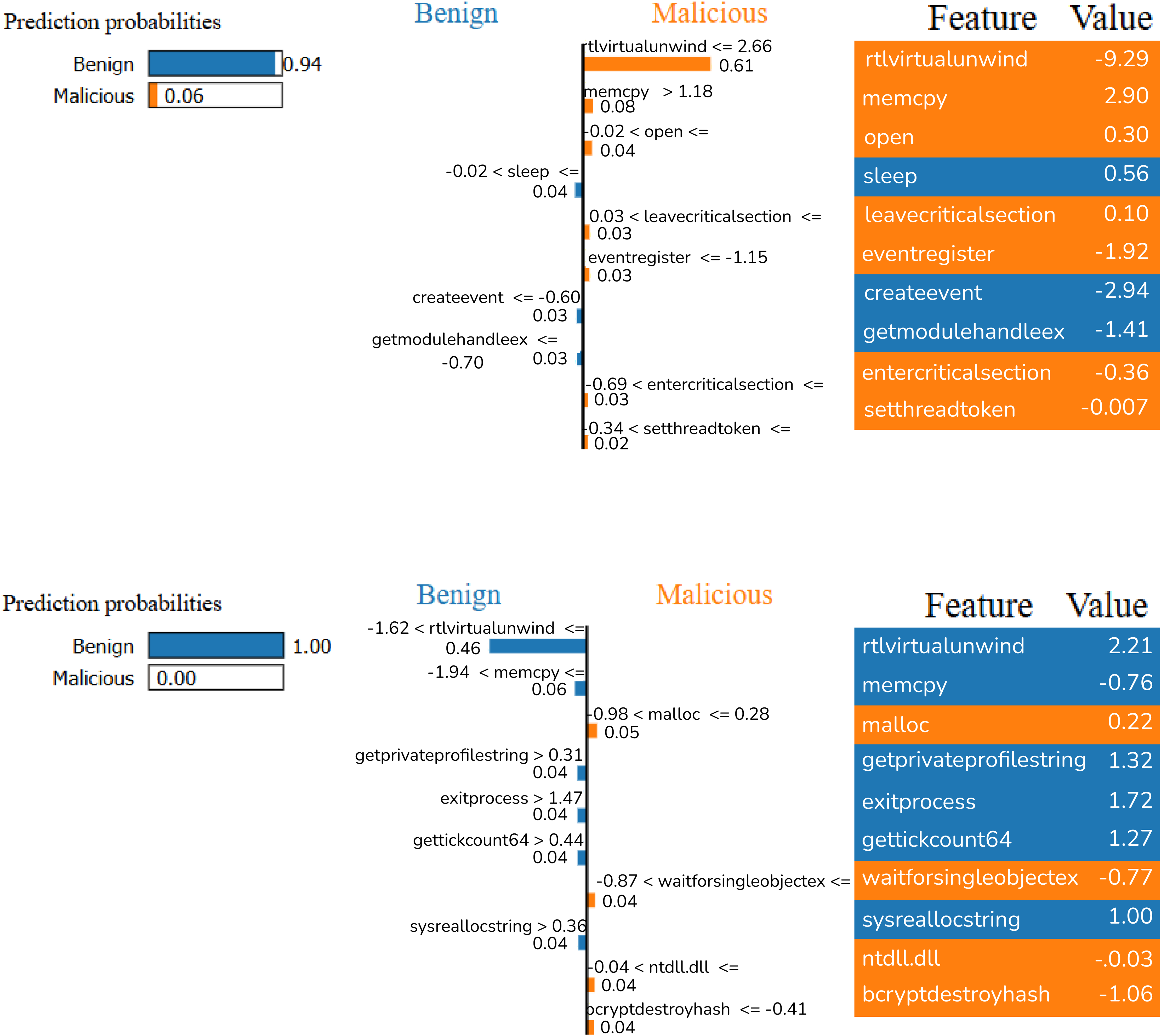
Figure 6 shows the analyses performed on two different random samples using the LIME method for XGB model. The LIME analysis visualizes the contribution of certain features to the classification decision to explain the model’s predictions. In the first analysis, it is seen that the model classifies the sample as Benign with 94% probability. These findings directly address RQ3 by revealing that API calls such as rtlvirtualunwind, memcpy, open, and sleep played a decisive role; especially the high values of rtlvirtualunwind and memcpy affected the model’s prediction. In the second analysis, the model labeled the sample as Benign with 100% probability. In this analysis, functions such as getprivateprofilestring, exitprocess, gettickcount64, and sysreallocstring were decisive. In both analyses, it is seen that the features that guide the model’s decisions are different; some features are associated with malware, while others show safe software characteristics. This shows that the model uses a dynamic decision mechanism and that certain function calls play a critical role in assessing the threat level.
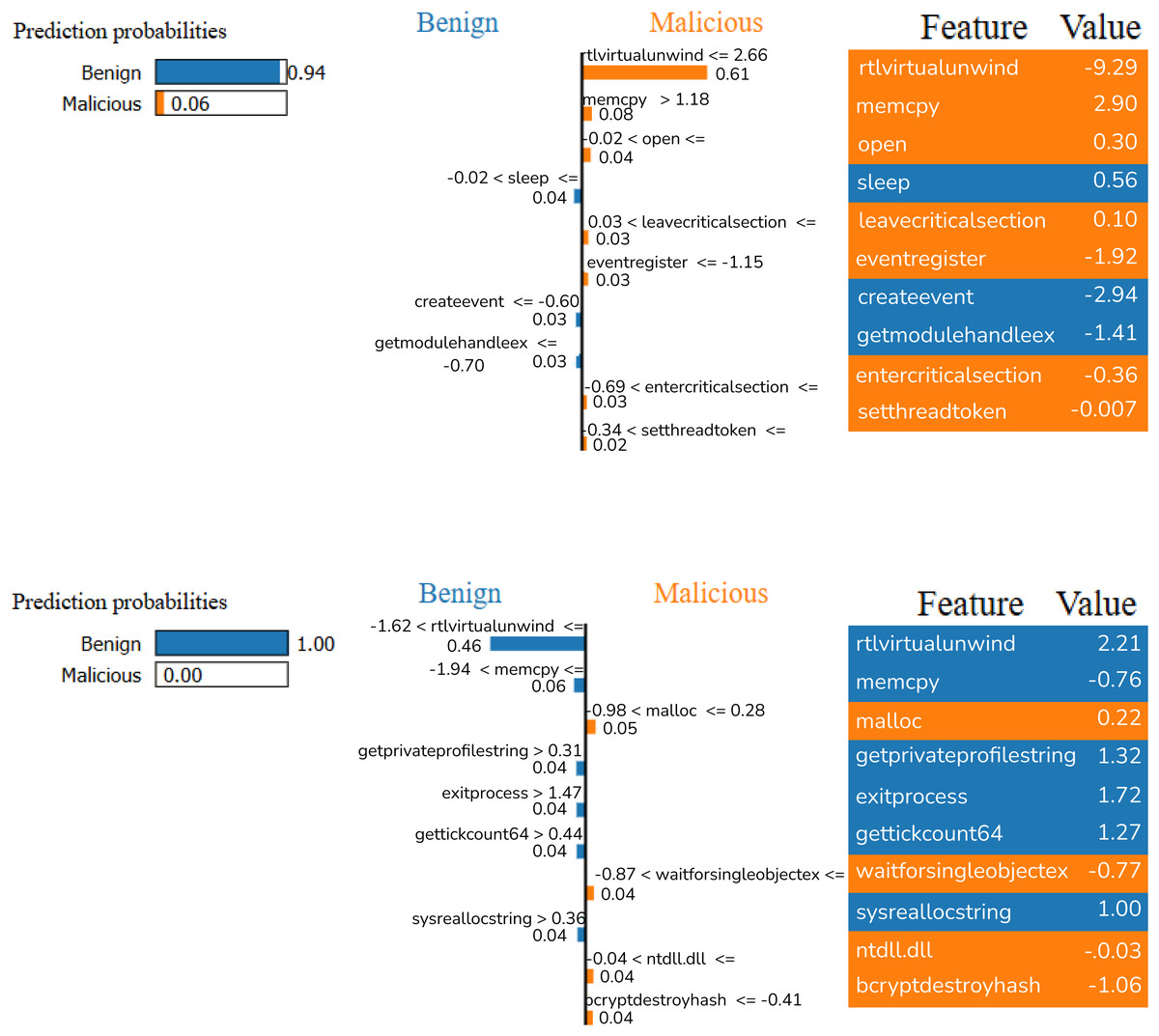
Figure 6: LIME results of XGB model with random samples.
Some of the functions mentioned,
rtlvirtualunwind is a function called in debugging and exception handling mechanisms and can be used by malware to check exceptions.
getprivateprofilestring is a Windows API call used to retrieve data from system configuration files and can be used by software trying to change system configurations. s study by providing a more accurate view of malware behavior.
exitprocess is a basic system call called when a process is terminated and can be used by malware to abruptly stop a process.
gettickcount64 returns the time elapsed since the system was started in milliseconds and can be used for time-based attacks or analysis detection.
sysreallocstring is a function used for memory management and can be exploited by malware trying to manipulate dynamic memory management.
assignprocesstojobobject is a function that used to limit system resources by assigning a process to a specific Job Object.
asn1berdecnull Used to parse NULL values when decoding Abstract Syntax Notation One (ASN.1) Basic Encoding Rules (BER).
_vswprintf_l One of the wide-character string creation functions, used to format strings in memory.
_beginthread Used to create multithreading, similar to _beginthreadex.
A comparative evaluation of the applied explainability techniques indicates that SHAP offers a globally consistent and theoretically grounded framework by assigning Shapley values to each feature, thereby enabling the identification of API calls and DLLs that systematically influence malware classification. This global perspective enhances the reliability of the interpretive analysis and allows for comprehensive assessment of the model’s behavior across the entire dataset. Conversely, LIME provides locally faithful, instance-specific explanations by approximating the decision boundary in the neighborhood of individual samples. Such localized analysis is particularly useful for illustrating why a specific executable is classified as malicious or benign, offering actionable insights at the case level. Overall, SHAP contributes to capturing the overarching importance of features with consistency, whereas LIME facilitates the interpretability of individual predictions. Their combined application ensures both global reliability and local transparency, thereby strengthening the trustworthiness of the proposed model in practical malware detection scenarios.
Conclusion
This study conducted a comprehensive comparative analysis of various machine learning and deep learning models for static malware classification. A range of models, from traditional algorithms like XGBoost, RF, and KNN to deep learning architectures such as CNN, LSTM, and GRU, were systematically evaluated. The methodology involved a rigorous preprocessing pipeline, including data augmentation, feature vectorization with CountVectorizer, feature selection using SelectKBest, and dimensionality reduction via PCA. Our experimental results, validated by statistical significance testing, revealed a nuanced performance landscape. The XGBoost model emerged as the overall top performer, achieving a statistically significant accuracy of 99.81%. This finding underscores the profound effectiveness of optimized gradient boosting methods on well-structured, high-dimensional feature sets common in static analysis. Concurrently, our proposed hybrid deep learning model, CNN-GRU-3, distinguished itself by achieving the best performance among all evaluated DL models (99.37%). Crucially, statistical analysis confirmed that this performance was a significant improvement over the baseline standalone CNN model, thereby validating our core hypothesis that synergistically combining CNNs for spatial feature extraction and GRUs for sequential pattern recognition is a highly effective strategy for this task. While acknowledging the superior accuracy of the simpler XGBoost model, we contend that the value of our more complex CNN-GRU-3 model is multifaceted. The application of XAI techniques, namely SHAP and LIME, on both the XGBoost and CNN-GRU-3 models provided deeper, complementary insights into their decision-making processes, directly addressing the black-box problem. This work, therefore, not only establishes strong performance benchmarks but also highlights a promising research direction towards building more robust, transparent, and potentially more generalizable malware detection systems. The findings provide a solid foundation for future explorations into both high-performance ensemble methods and advanced, interpretable deep learning architectures in the field of cybersecurity.