
Sliding window higher-order cumulants for detection of eye blink artifact from short segments of single-channel EEG
- Published
- Accepted
- Received
- Academic Editor
- Shibiao Wan
- Subject Areas
- Adaptive and Self-Organizing Systems, Algorithms and Analysis of Algorithms, Brain-Computer Interface, Scientific Computing and Simulation
- Keywords
- Artifact detection, Electroencephalogram (EEG), Eye blink artifacts, Sliding window higher-order cumulants (HOCs), Short segments
- Copyright
- © 2025 Wang et al.
- Licence
- This is an open access article distributed under the terms of the Creative Commons Attribution License, which permits using, remixing, and building upon the work non-commercially, as long as it is properly attributed. For attribution, the original author(s), title, publication source (PeerJ Computer Science) and either DOI or URL of the article must be cited.
- Cite this article
- 2025. Sliding window higher-order cumulants for detection of eye blink artifact from short segments of single-channel EEG. PeerJ Computer Science 11:e3249 https://doi.org/10.7717/peerj-cs.3249
Abstract
Background
The prevalence of single-channel electroencephalogram (EEG) is increasing. However, eye blink artifacts can contaminate EEG signals, potentially impacting their clinical utility.
Method
This study presents a sliding window higher-order cumulant (HOC) method for accurate blink artifact detection. The method operates in two steps. First, preliminary detection of blink artifacts is achieved by computing HOCs within the sliding windows of contaminated EEG. Second, the method identifies blink peaks within the detected intervals and further adjusts the detection results using the peaks.
Results
The study compares the effectiveness of the sliding window HOC method with the existing variational mode extraction (VME) and multi-window summation of derivatives within a window (MSDW) methods using semi-simulated and real data. The comparison results show that, for semi-simulated data, the sliding window HOC method exhibits the highest Youden index values in terms of the direct accuracy metrics. When it comes to the indirect metrics of artifact reduction effectiveness based on the three detection methods, the sliding window HOC method has the highest correlation coefficient (CC) (0.935 vs. 0.914, 0.909), the lowest relative root mean square error (RRMSE) (0.128 vs. 0.186, 0.225), and the lowest mean absolute error (MAE) (1.634 vs. 1.770, 1.748). For real data, it yields the highest MAE ratio of the lower-to-higher frequency bands among three datasets. The algorithm also demonstrates computational efficiency with millisecond-level resolution.
Discussion
The sliding window HOC method provides superior detection performance and greater robustness. The presented method provides a solid foundation for effectively removing blink artifacts in single-channel EEG.
Introduction
The prefrontal single-channel electroencephalography (EEG) system, offering portable and mobile monitoring capabilities, holds significant application value in neuroscience research and clinical diagnosis (Ali et al., 2022). As the core regulatory hub of the brain, the prefrontal cortex governs higher-order neural functions including executive control, decision-making, and motor coordination, while simultaneously participating in complex cognitive processes such as emotion regulation, attention modulation, and mental state integration. Through real-time monitoring of neural electrical signals in this region, researchers can accurately identify neural activity patterns associated with transitions from relaxed to focused states, facilitating an objective and quantifiable cognitive function assessment framework (Ahn, Ku & Kim, 2019). In clinical diagnostics, prefrontal EEG signal analysis is widely applied for biomarker detection in neurological disorders. It demonstrates significant value in early screening and disease monitoring of movement disorders, executive dysfunction syndrome, Foster-Kennedy syndrome, and other neurological conditions, providing reliable neuroelectrophysiological evidence for precision medicine (Dora & Biswal, 2020). However, similar to multichannel EEG, single-channel EEG remains susceptible to artifacts, particularly eye blinks, which can significantly affect prefrontal EEG and are difficult to manage or overcome experimentally (Shahbakhti et al., 2019).
For attenuating blink artifacts in single-channel EEG, various decomposition methods are commonly employed, including singular spectrum decomposition (Maddirala & Veluvolu, 2022a; Mary Judith, Baghavathi Priya & Mahendran, 2022; Yedukondalu & Sharma, 2023), wavelet decomposition (Maddirala & Veluvolu, 2022a; Sahoo & Mohapatra, 2022), empirical mode decomposition (Yan & Wu, 2022), and independent component analysis (Mary Judith, Baghavathi Priya & Mahendran, 2022; Sahoo & Mohapatra, 2022). However, such decomposition-based methods typically apply global filtering across the entire contaminated EEG signal instead of specifically targeting artifact-contaminated intervals. This approach may inadvertently remove both artifact-corrupted and intact neural components. Notably, emerging evidence suggests that precise temporal localization of blink events significantly improves artifact suppression efficacy while enhancing preservation of genuine neural activity (Maddirala & Veluvolu, 2022a, 2022b; Gao et al., 2023). This paradigm shift from global to targeted artifact removal thus represents a promising direction for improving EEG signal quality.
Currently, the primary methods to detect blink artifacts involve amplitude thresholding (Nolan, Whelan & Reilly, 2010), template matching (Valderrama, de la Torre & Van Dun, 2018), peak detection (Shahbakhti et al., 2021a), and derivative summation detection (Chang et al., 2016). However, most of these methods require empirically preset conditions, and few have explored whether the boundaries of blink artifact intervals are accurately recognized. Amplitude thresholding, which is based on a priori estimation of blink artifact amplitude, achieves the detection of blink peaks and thus blink position localization, but it does not accurately identify blink intervals. The peak detection method identifies the peaks using the variational mode extraction (VME) method (Shahbakhti et al., 2021a), and the boundaries of the artifact intervals are determined based on an empirical estimate of the blink interval width (400 ms) using the identified peaks. The template matching algorithm (Valderrama, de la Torre & Van Dun, 2018) was proposed to detect and eliminate eye blinks using an automatic threshold and template estimation. However, like the VME method, its blink template is fixed at 1,400 ms and does not precisely identify the boundaries of the exact blink interval. The method for multi-window detection of derivative summation (MSDW) can identify the start and end points of blink intervals (Chang et al., 2016). However, it requires the assumption that blink artifacts exhibit a triangular shape.
Therefore, it is necessary to establish an assumption-free detection approach capable of adaptively and more precisely identifying blink artifacts of varying durations by exploiting the inherent characteristic distinctions between EEG signals and blink artifacts. Hence, considering the differences in the non-Gaussian properties of EEG signals and blink artifacts, higher-order cumulants (HOCs) are introduced for distinguishing blink artifacts from EEG signals without a priori assumptions. Currently, the application of HOCs in ocular artifact processing still primarily involves combining them with various signal decomposition methods as previously mentioned, including blind source separation (Jamil, Jamil & Majid, 2021; Çınar, 2021; Gao et al., 2023), variational mode decomposition (Bisht et al., 2024), empirical mode decomposition (Teng et al., 2021), canonical correlation analysis (Yang et al., 2017), and wavelet transform (Shahbakhti et al., 2021b; Islam, Ghorbanzadeh & Rastegarnia, 2021). These methods identify and remove artifact components by calculating HOC values of the decomposed signals. However, HOCs still evaluate the decomposed signal components in their entirety. As previously mentioned, this global processing approach may compromise neural activity information within artifact-free segments. Nevertheless, these studies have laid a theoretical foundation for the effectiveness of HOCs in extracting non-Gaussian signal features, and it is precisely based on these validated findings that they provide the research impetus for our exploration into using HOCs directly for the accurate detection of blink artifacts.
This article presents a sliding window HOC method for detecting blink artifacts, which offers two advantages: First, by incorporating HOCs, it can automatically distinguish between EEG signals and blink artifacts based on their non-Gaussian characteristics, effectively overcoming the limitations imposed by empirically preset conditions. Second, the sliding-window computation strategy generates time-varying HOC series that allow precise localization of the onset and offset boundaries of blink artifacts. Specifically, a sliding window is applied to the contaminated EEG signals, and HOCs are computed window by window. These HOC values are then used to preliminarily estimate the intervals of the blink artifacts based on the local maxima. Subsequently, the pre-detected intervals are further adjusted by incorporating the peaks of the blink artifacts within those intervals to improve the precision of the final detection. This study also evaluates the efficacy of the sliding window HOC method using semi-simulated and real data. The method is compared with the existing eye blink artifact detection methods, including VME and MSDW.
Materials and Methods
HOCs
Higher-order cumulants (HOCs) are statistical measures that extend the concept of variance (a second-order cumulant) to quantify higher-order dependencies and non-Gaussian characteristics in signals (Bakouch, 2010; Antari et al., 2011). The kth-order cumulant of a random variable is derived from its characteristic function , defined as:
(1) where is the probability density function of . The second characteristic function is the natural logarithm of :
(2)
The kth-order cumulant is then obtained as the kth derivative of evaluated at ω = 0:
(3)
For a random process ], its characteristic functions are calculated as follows:
(4)
(5) The -order cumulants of are obtained by
(6) where
From the above definition and further calculations, it can be seen that the first-order cumulants of Gaussian-distributed random processes are equal to the mean, the second-order cumulants are equal to the variance, and the higher-order cumulants (for order greater than 2) are zero. Therefore, HOCs are insensitive to Gaussian-distributed signals. Due to the Gaussian characteristics of EEG signals, their amplitude distribution shares similarities with the statistical characteristics of the Gaussian distribution (Chen, 2014). As a result, their HOCs closely approach 0. Conversely, eye blink signals do not adhere to the Gaussian distribution’s characteristics, resulting in significantly larger values for their HOCs. In signal processing, the third-order and fourth-order cumulants are most commonly employed. Considering the lower computational complexity of the third-order cumulants when compared to the fourth-order (Khoshnevis & Sankar, 2020), this study adopts third-order cumulants for analysis.
The sliding window HOC method
Based on the difference in Gaussian characteristics between EEG signals and eye blink artifacts, this article proposes a sliding window higher-order cumulant analysis method for detecting eye blink artifacts in EEG signals. In this approach, the target signal to be detected is the blink artifact, whereas the EEG background activity serves as the noise source. HOCs are employed to suppress the EEG noise, enabling the detection of the blink artifacts.
The main steps of our proposed sliding window HOC with further adjustments are summarized in Algorithm 1. Assuming that the contaminated EEG time series is . The sliding window HOC are defined as
(7) where denotes the HOC function and is the sliding window length. represents the HOC value of the th sliding window of the contaminated EEG signals. Due to the difference in their Gaussian distributions, the HOC values increase when an eye blink signal is present within the sliding window. This enables the localization of the eye blink artifacts and facilitates the detection of these artifacts.
| Input: Contaminated EEG ( ), , , , |
| Output: Final detected eye blink intervals [ ] |
| Initialization: |
| {Step 1: Preliminary detection of blink intervals} |
| 1: for |
| 2: |
| 3: end |
| 4: |
| 5: |
| 6: |
| 7: {Points within of are considered to be one artifact segment} |
| 8: |
| 9: |
| 10: Step 2: Further adjustments to detected blink intervals (exemplified by D1D2 in Fig. 2)} |
| 11: |
| 12: |
| 13: |
| 14: |
| 15: |
| 16: while |
| 17: |
| 18: end |
| 19: while |
| 20: |
| 21: end |
| 22: while |
| 23: |
| 24: end |
| 25: while |
| 26: |
| 27: end |
| 28: |
| 29: |
| 30: return |
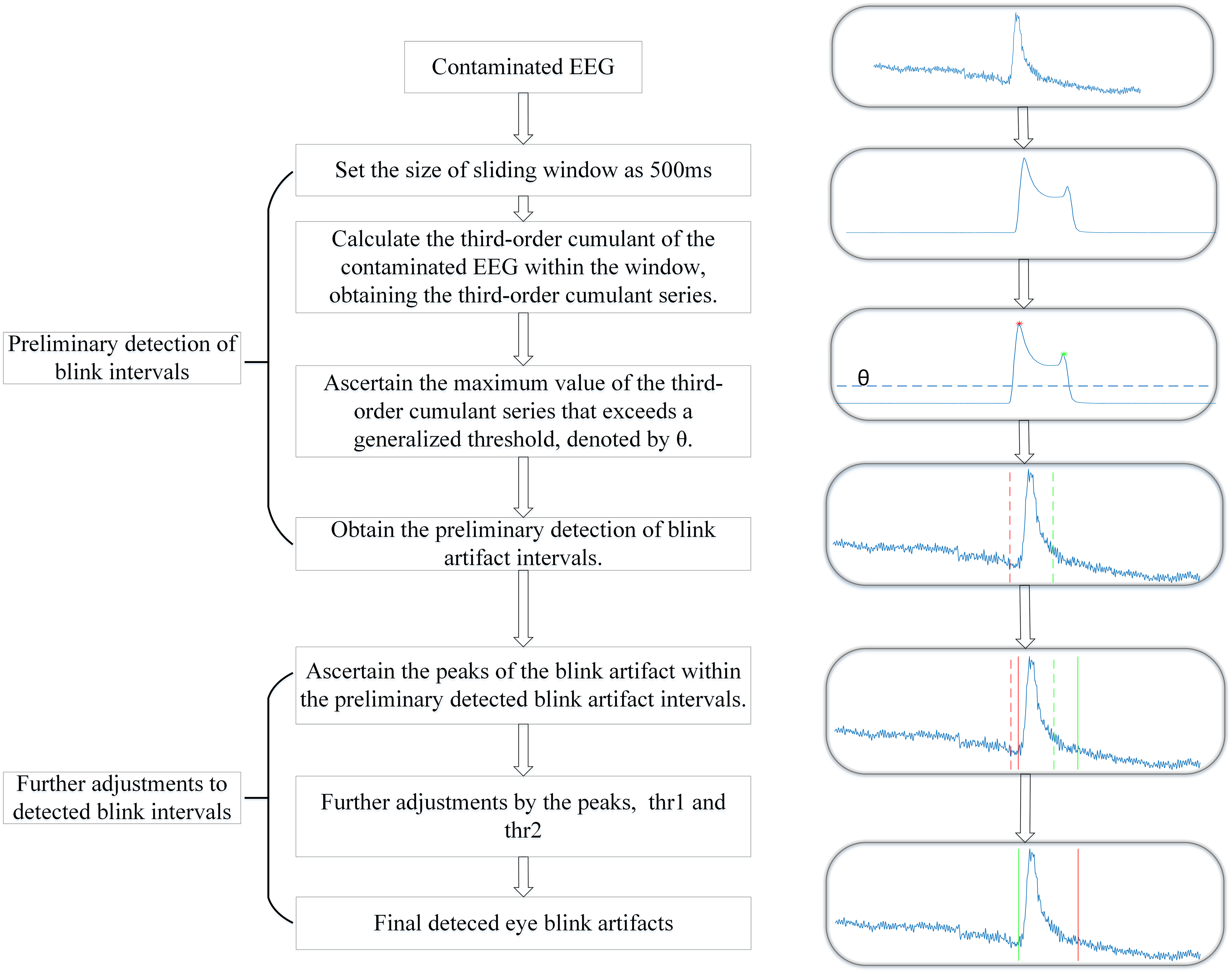
Figure 1 shows the block diagram of the sliding window HOC method, which is executed in two main steps: first, preliminary detection of eye blink intervals, and second, further adjustment of the detected intervals.
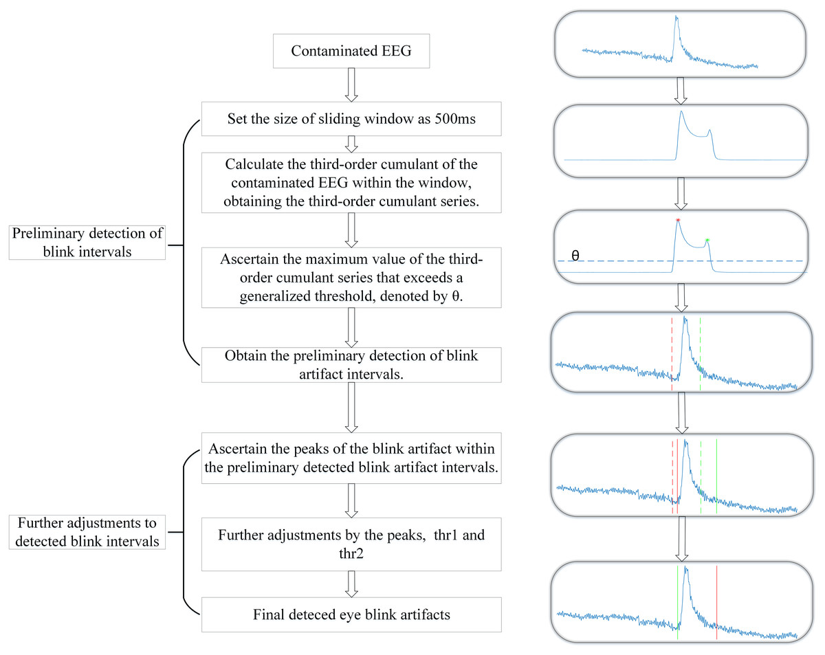
Figure 1: The block diagram of sliding window higher-order cumulant (HOC) method.
Preliminary detection of blink intervals
The preliminary detection of blink intervals refers to the preliminary localization of blink artifact intervals based on the sliding window HOC method, involving the determination of parameters that affect the accuracy of detection outcomes. The key parameter to be determined in this step is the size of the sliding window ( ). Given that the typical duration of blink artifacts ranges from 100 to 500 milliseconds (Chang et al., 2016), the preliminary detection phase must address two key requirements: first, ensuring the rough identification of time intervals containing blink artifacts; and second, guaranteeing that these initially detected intervals cover the peak positions of blink artifacts. This coverage is a critical parameter for subsequent further adjustment procedures. Based on these considerations, is empirically set to 500 milliseconds.
After the sliding window HOCs have been calculated based on the specified order and window size, the intervals containing blink artifacts are determined by identifying local maxima in the sliding-window HOCs that exceed a universal threshold (Chavez et al., 2018; Shahbakhti et al., 2021a). The universal threshold is calculated as follows:
(8) where Czzz represents the sliding-window HOCs, and N denotes the length of Czzz series. After zeroing out Czzz values below threshold θ, we employ the function to identify local maxima, where contains the peak amplitudes and indicates their corresponding time indices. When the interval between two adjacent maxima is less than 0.5 * Fs sampling points (equivalent to 500 ms), these peaks are considered to belong to the same blink artifact segment. This approach enables preliminary determination of the blink artifact’s and , as detailed in Algorithm 1.
Further adjustments to detected blink intervals
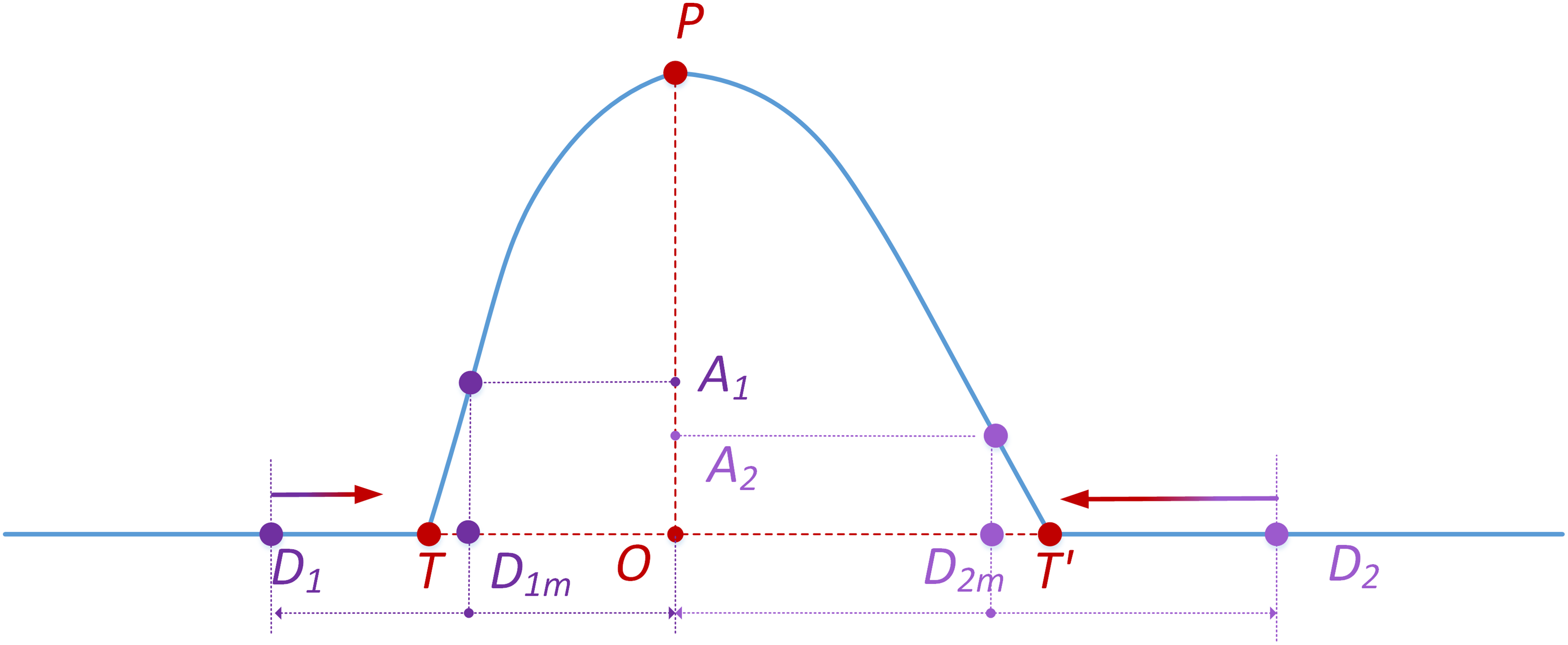
To address the detection deviation caused by the fixed sliding-window size (500 ms) in the preliminary detection stage-which fails to adapt to the dynamic variations in blink artifact durations-further adjustments are implemented. These adjustments dynamically refine detection intervals based on blink peak positions (see Fig. 2). The purpose of the two parameters, denoted as and , is to optimize the detected blink intervals and estimate the precise temporal boundaries of eye blink artifacts. These parameters are intrinsically associated with the asymmetric characteristics of blink waveforms: governs detection sensitivity for the leading edge, while controls trailing edge adjustment. Their values dynamically adapt to slope variations determined by blink width and peak amplitude. Through an iterative optimization approach using a stepwise approximation algorithm for artifact boundary refinement, precise localization of blink artifact intervals is ultimately achieved.
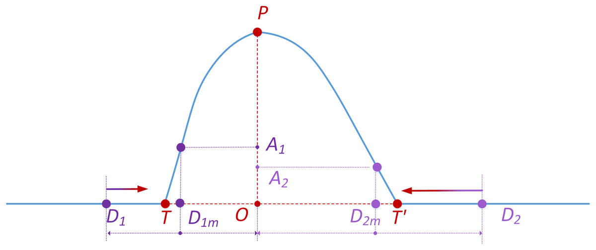
Figure 2: Schematic diagram of the further adjustment to the detected eye blink interval.
As illustrated in Fig. 2, point P represents the peak of the actual blink artifact within the detected blink interval, and point O denotes its location. While TT’ refers to the actual blink artifact interval, D1D2 represents one example of preliminarily detected blink intervals. The primary purpose of further adjustment is to draw D1D2 closer to TT’. Exemplified by D1D2, the procedure is as follows: for D1 of the D1D2, locate the centroid D1m of the D1O and calculate the magnitude of its corresponding actual blink signal. If the ratio ( ) of this magnitude (A1O) to the peak value (PO) is less than the predetermined threshold ( ), point D1 moves one sample point to the right until exceeds , and then it stops moving. For D2 of the D1D2, locate the centroid D2m of the D2O and determine the corresponding magnitude. If the ratio ( ) of the magnitude (OA2) to the peak value (OP) is less than the set threshold ( ), point D2 shifts one sample point to the left until exceeds , after which it comes to a stop. This process yields the final refined start and end points of the blink artifacts after further adjustment, which represent the algorithm’s ultimate determination of blink artifact boundaries.
Data
The proposed sliding window HOC method for the blink artifact detection was validated using semi-simulated and real data.
Semi-simulated data
Semi-simulated data are generated using the following mixing model:
(9) where is the artifact-free EEG signal, is the eye blink electrooculogram (EOG) artifact signal, and represents the contaminated EEG signals. Parameter controls the signal-to-noise ratios (SNR) in semi-simulated datasets. The objective of the sliding window HOC method is to determine the temporal location and boundaries of within .
In this article, pure blink signals were recorded using the vertical electrooculographic channels of the Neuroscan recording system (Compumedics Limited, Melbourne, Australia). To enhance signal quality, blink recordings were low-pass filtered at 10 Hz. Artifact-free EEG segments (485 epochs of 3-s duration) were selected from Klados & Bamidis (2016), originally recorded according to the 10–20 international system at 200 Hz sampling frequency. Given blink durations predominantly ranging from 100–500 ms, collected blink artifacts were categorized into five duration groups: 100, 200, 300, 400, and 500 ms. Semi-simulated datasets with varying SNR levels were generated by contaminating artifact-free EEG signals with blink artifacts.
Real data
The proposed algorithm was also evaluated using the real data. We collected 1676 3-s EEG segments from frontal channels, sourced from three public databases (Chavarriaga & del Millan, 2010; Ofner et al., 2017; Cavanagh et al., 2019). Utilizing multiple databases allowed investigation of the algorithm’s adaptability across different recording conditions. Database characteristics are summarized in Table 1.
| Database | Data1 (Ofner et al., 2017) | Data2 (Chavarriaga & del Millan, 2010) | Data3 (Cavanagh et al., 2019) |
|---|---|---|---|
| Sampling rate | 512 Hz | 512 Hz | 500 Hz |
| Selected contaminated EEG channel | FP1 | FP1 | FP1 |
| Recording system | g.tec medical engineering GmbH | Biosemi active two system | Synamps2 system |
| Number of subjects | 15 | 6 | 14 |
| Number of segments | 708 | 324 | 644 |
Methods under comparison
The proposed algorithm is compared with VME and MSDW to ascertain its effectiveness for detecting eye blink artifacts in single-channel EEG signals.
VME
The VME algorithm detects blink artifacts by first estimating the contaminated EEG signal to identify the peak of the blink artifact. Subsequently, the interval of the blink artifact is determined with a 125 ms pre-peak and a 375 ms post-peak window.
MSDW
The MSDW technique computes the summation of the first-order derivatives of the raw signal within the sliding window for the filtering of EEG ripples, thereby identifying blink artifacts. The method necessitates manual threshold setting, and we assessed its efficacy at the threshold value of 130 suggested by the authors.
Performance metrics
In order to assess the accuracy of blink artifact detection, both direct accuracy metrics and indirect artifact reduction effectiveness metrics are employed.
Accuracy metrics
Accuracy metrics offer a straightforward means of evaluating detection algorithms. To assess the accuracy of the blink detection methods in more detail, both rough and fine assessment metrics have been used.
Rough assessment metrics are employed to evaluate the algorithm’s ability to locate blink artifacts. A detection is classified as a rough true positive ( ) if it overlaps with any actual blink artifact, and as a rough false positive ( ) when no overlap occurs with genuine blink regions. These metrics include the rough true positive rate ( ) and rough false positives per sample ( ), calculated as follows:
(10)
(11) where stands for the number of correctly detected eye blinks, while denotes the total number of actual eye blinks. indicates the number of false positive detections, and represents the total duration (in samples) of artifact-free EEG. Since true negatives (TN) are undefined for continuous signals (Valderrama, de la Torre & Van Dun, 2018), is evaluated over temporal intervals, making it equivalent to the false positive rate (FPR). However, these rough metrics are inadequate for assessing endpoint recognition precision of blink artifacts.
The fine assessment metrics are designed to assess whether the method can accurately estimate the boundaries of the eye blink artifacts. Therefore, we define the fine assessment metrics by introducing the concept of “error tolerance” (Chang et al., 2016), based on the fact that blink artifacts blend with genuine EEG signals, creating boundary ambiguity that necessitates a permissible error range to avoid overly stringent determinations. Figure 3 illustrates the basic concept of error tolerance. “Ground truth” refers to the exact range of an eye blink artifact. If an error tolerance is specified for the two boundaries of the artifact, actual errors (false positives or false negatives) found within these “error tolerance” ranges are considered part of correctly detected artifact ranges. The error tolerance includes false negative tolerance (FN tolerance) and false positive tolerance (FP tolerance). FN tolerance is defined as the ratio of the tolerated FN region to the length of the ground truth segment for each artifact, since the width of each artifact varies. In contrast, the FP tolerance is defined as a fixed time interval (in seconds) extending from the boundaries of the ground truth segment for each artifact. In our implementation, FP tolerance ranges from 0 to 0.1 s and FN tolerance ranges from 0 to 40 percent of the ground truth segment (Chang et al., 2016). Specifically, the FN tolerance range of 0–40% is chosen based on the physiological characteristics of blink artifacts and signal ambiguity. Since blink artifact waveforms exhibit gradual rising and falling slopes, strictly defining their boundaries could lead to missed detections. A 40% FN tolerance means allowing a 40% margin of error relative to the artifact’s duration near its boundaries (e.g., allowing an 80 ms tolerance for a 200 ms artifact). This range covers the transition zone between artifacts and EEG signals in most practical cases, ensuring detection sensitivity while preventing excessive leniency that could introduce significant noise interference. The FP tolerance range of 0.0–0.1 s is chosen to effectively distinguish blink artifacts from other transient interference. A 0.1-s FP Tolerance accommodates the duration of brief disturbances while avoiding misclassification of longer noise (such as motion artifacts) as blinks. In addition, the figure also shows four different possible detected eye blinks.
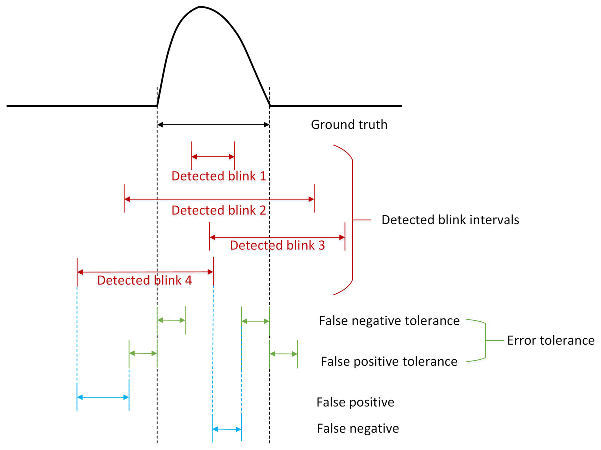
Figure 3: A schematic diagram illustrates the concepts of error tolerance and the positive detected blink intervals.
Based on the concept of “error tolerance”, we define the fine assessment metrics which include the fine true positive rate ( ) and the fine false positives per sample ( ).
(12)
(13) where , and stand for the correct, missed and false duration in samples of detected eye blinks, respectively. The is still the total duration in samples of the pure EEG.
Artifact reduction effectiveness metrics
Artifact reduction effectiveness metrics can serve as an indirectly assessment of blink detection accuracy. Better removal of blink artifacts alongside better retention of valid EEG indicates more accurate recognition of blink artifacts. The study conducts indirect verification of artifact detection accuracy by applying the same wavelet denoising method after the three blink artifact detection algorithms. Specifically, the discrete wavelet transform (DWT) is used to filter the contaminated intervals using the db4 mother wavelet at a decomposition level of 3. To quantify the artifact reduction performance, we use the correlation coefficient ( ) and the relative root mean square error ( ) in the time domain. Additionally, the mean absolute error ( ) is employed in the frequency domain.
can reflect the ability to perserve the original EEG signal during the denoising process. is calculated as
(14) where and are the pure EEG and filtered EEG signals, and are the covariance and standard deviation, respectively. The closer is to 1, the better the noise reduction.
is defined as
(15) where and represent the root mean square of the true and denoised EEG signals, respectively, and for an effective artifact reduction approach, the RRMSE value will be low.
MAE is employed to evaluate the performance in the frequency domain. and are the power spectrum of the contaminated and rectified EEG respectively. The MAE is defined as follows:
(16) where refer to the frequency range of a particular band.
For semi-simulated data, where the ground truth is known, MAE is used to evaluated EEG retention across the full frequency range (1–40 Hz) after artifact reduction. Results indicate effective artifact reduction, reflected in small MAE values. For real data, however, the lack of ground truth makes it impossible to calculate CC and RRMSE. MAE across the full frequency range (1–40 Hz) is also incalculable. Instead, MAE was always computed within the band due to blink artifact frequencies extending beyond the band (Noorbasha & Sudha, 2021; Yedukondalu & Sharma, 2023). It should be noted that insufficient artifact removal can still result in low MAE values in the α band. For instance, an MAE value of 0 in the band without artifact reduction signals adequate EEG preservation, not complete artifact elimination. Thus, we employed the MAE ratio ( ) of the low frequency band (1–10 Hz) to the high frequency band (10–40 Hz). This metric evaluates the algorithm’s efficacy in eliminating artifacts while preserving EEG signals.
Determination of parameters
The proposed sliding-window HOC method requires the optimization of two key parameters, and , designed to refine the detected blink intervals and estimate the optimal temporal range of eye blink artifacts. To systematically determine the optimal and values, we conducted an extensive parameter selection study using semi-simulated data. We generated a total of 108 semi-simulated contaminated EEG signal segments by systematically adjusting signal parameters: setting the SNR across 11 levels (−8 to 2 dB) and varying blink durations across five durations (100, 200, 300, 400, and 500 ms). This process constructed a comprehensive dataset comprising 108 × 11 × 5 samples for the determination of the optimal combination for parameters and . For each threshold combination, we computed and to evaluate detection performance across different noise conditions. The optimal threshold combination was identified by maximizing the Youden index, derived from receiver operating characteristic (ROC) curve analysis, ensuring a balanced trade-off between sensitivity and specificity. This rigorous parameter optimization framework enhances our method’s adaptability to diverse blink dynamics while maintaining robustness against noise interference.
Results
Results of parameters determination
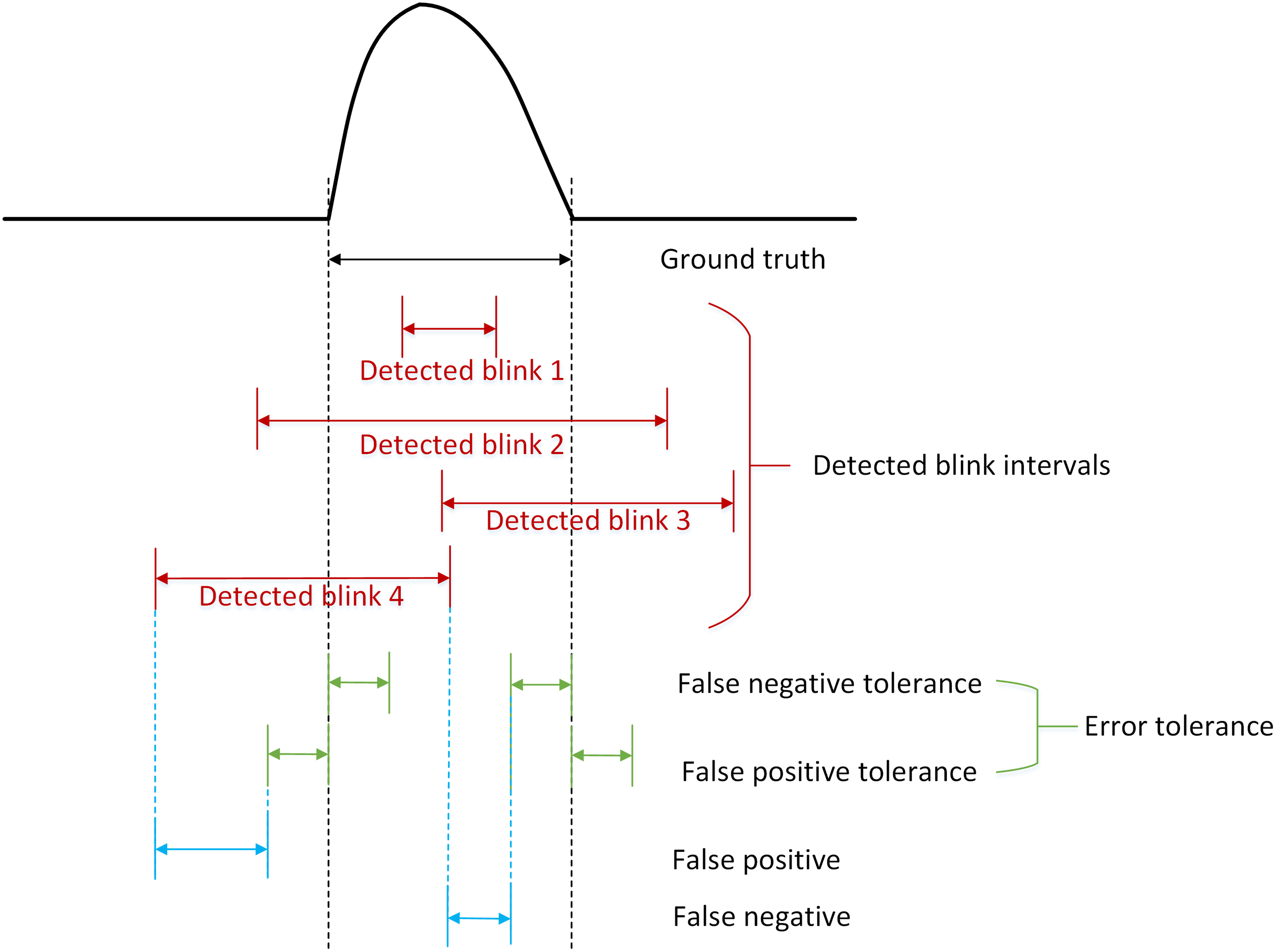
The parameters of the sliding window HOC method include and . For the chosen semi-simulated data (containing varying blink artifact intervals and different SNRs), we calculated the mean values of and false positives per second across different combinations of and , then plotted corresponding ROC curves. As shown in Fig. 4, the ten colored lines indicate values ranging from 0.0 to 0.9, while the ten circles along each line (arranged top to down) correspond to values from 0.0 to 0.9. These collectively form the ROC curves for all parameter combinations. The maximum Youden index value of the ROC curve is 0.9422, corresponding to = 0.9679 and = 0.0257. This optimal point (indicated by the third circle from the top on the bold purple line) represents the combination = 0.4 and = 0.2. Thus, and were identified as the optimal parameters for subsequent analysis.
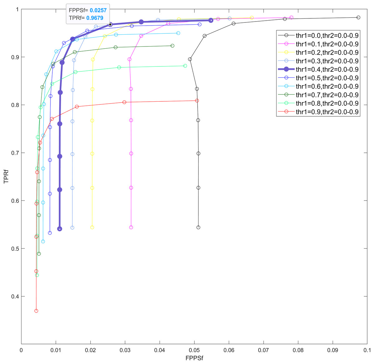
Figure 4: ROC curves under different combinations of thr1 and thr2, where both thresholds range from 0.0 to 0.9 (step size: 0.1).
Each colored line represents a distinct thr1 value, while the 10 circles along each line (from top to bottom) correspond to thr2 values. TPRf, fine true positive rate. FPPSf, fine false positives per sample.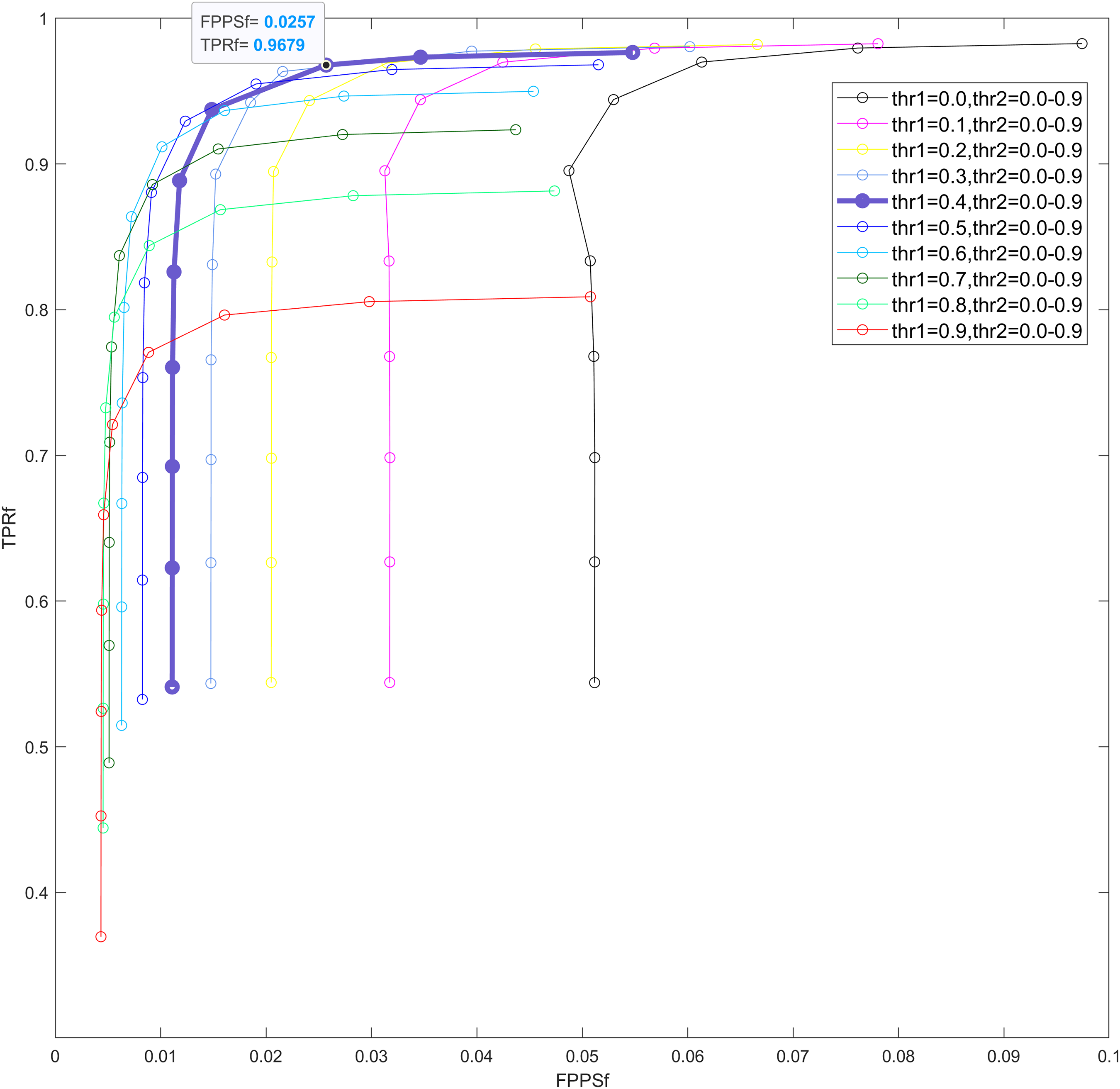
Results of semi-simulated data
Results from the semi-simulated data involved comparing the precision of three distinct blink detection methods and the denoising effectiveness generated based on these detection methods.
Table 2 illustrates the rough accuracy metrics for the proposed sliding window HOC, VME, and MSDW methods across various SNRs. The results show that the proposed method achieved consistently higher Youden index values across all SNRs, indicating superior rough detection accuracy. Figure 5 presents the ROC curves of the fine assessment metrics of each method under varying FP and FN tolerances. These results indicate that the proposed method exhibited the highest at any given .
| SNR | SNR ≤ −4 | −4 < SNR < 0 | 0 dB | |
|---|---|---|---|---|
| TPRr | Sliding window HOCs | 1.000 | 0.993 | 0.945 |
| VME | 0.990 | 0.976 | 0.853 | |
| MSDW | 0.266 | 0.215 | 0.192 | |
| FPPSr | Sliding window HOCs | 2.08E−04 | 2.39E−04 | 2.81E−04 |
| VME | 3.49E−03 | 4.51E−03 | 5.30E−03 | |
| MSDW | 1.29E−04 | 1.28E−04 | 1.26E−04 | |
| Youden index | Sliding window HOCs | 1.000 | 0.993 | 0.945 |
| VME | 0.987 | 0.971 | 0.847 | |
| MSDW | 0.266 | 0.215 | 0.192 |
Note:
Rough true positive rate (TPRr), rough false positives per sample (FPPSr) and the Youden index obtained at different SNRs with the sliding window HOC method, the VME method, and the MSDW method.
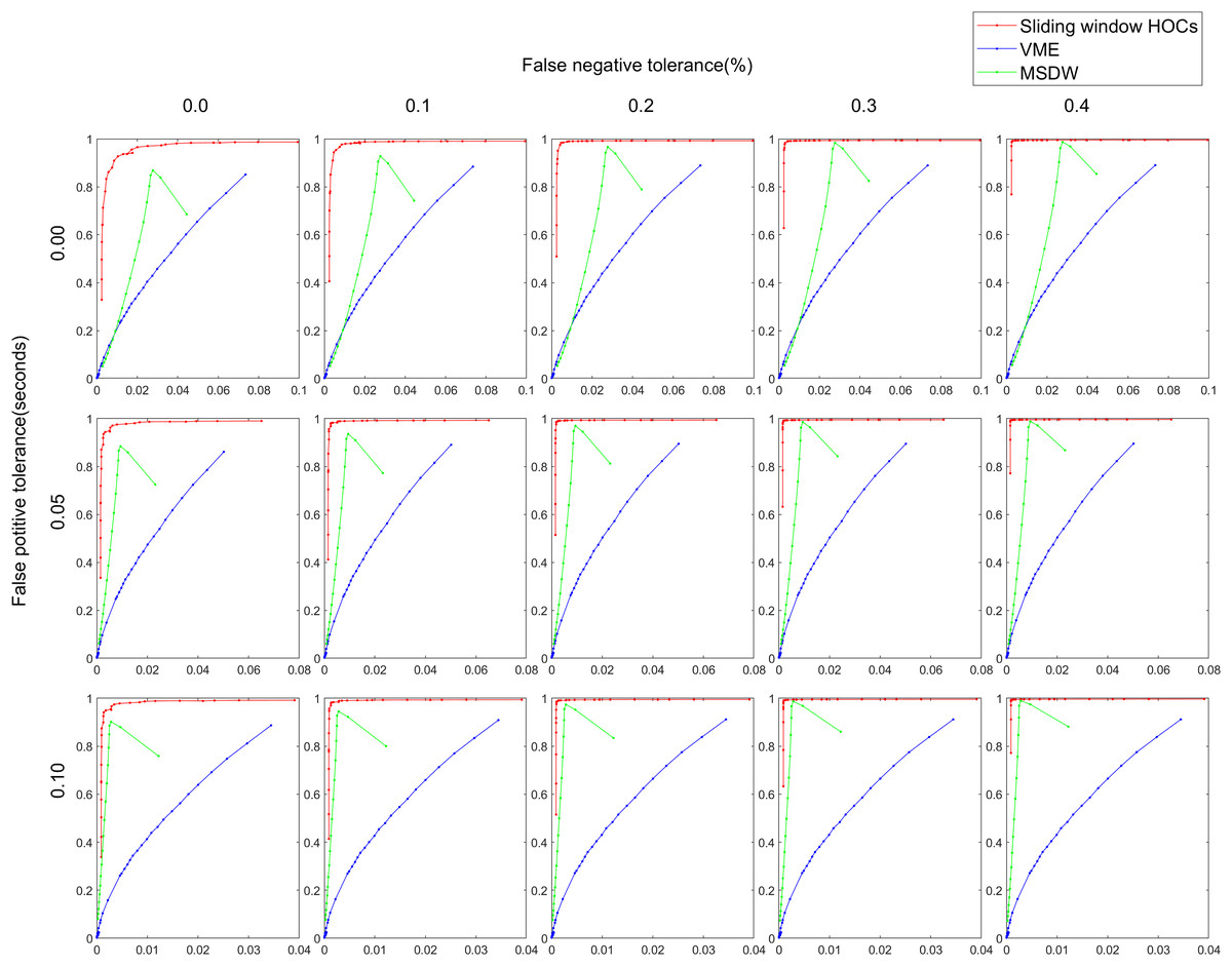
Figure 5: ROC curves with respect to different pairs of false positive tolerances and false negative tolerances in the estimation of the artifact ranges. The false positive tolerance ranges from 0.00 to 0.10 (step size: 0.05), while the false negative tolerance ran.
The abscissa of each curve represents the fine false positives per sample (FPPSf), and the ordinate represents the fine true positive rate (TPRf).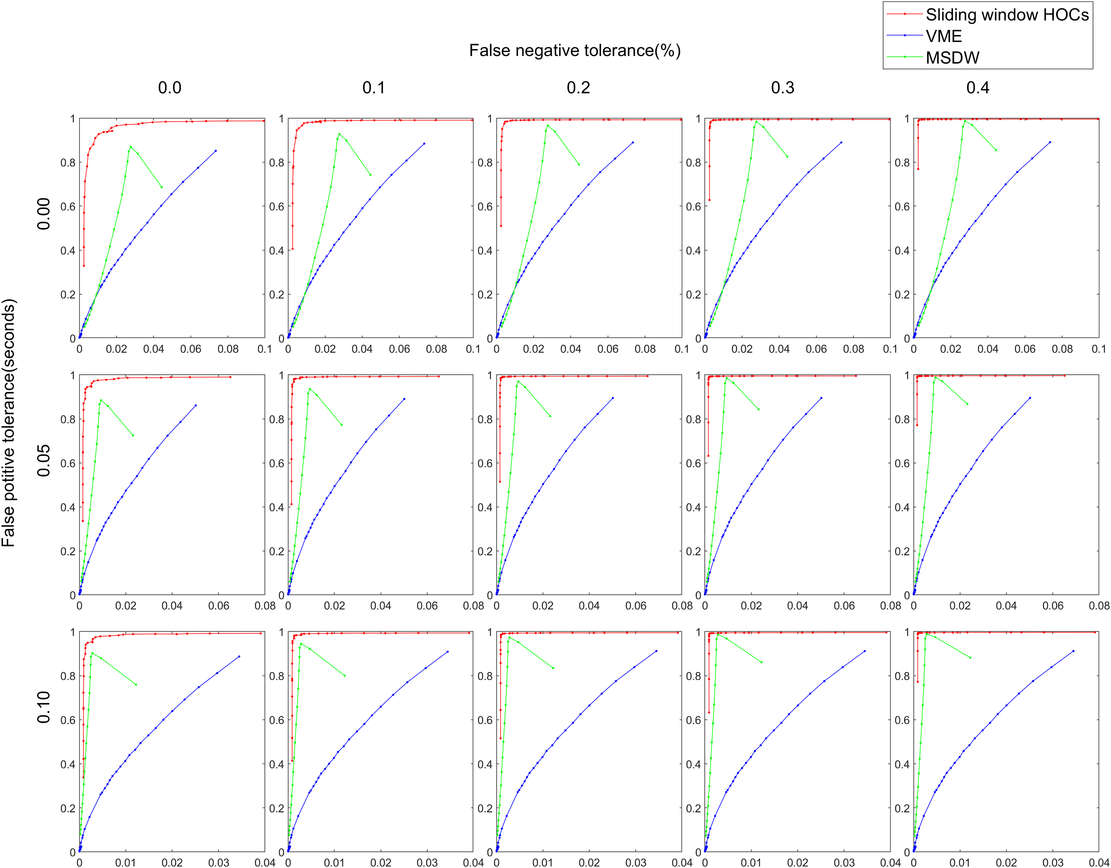
Figure 6 and Table 3 display indirect artifact reduction effectiveness metrics for the semi-simulated data, including CC, RRMSE and MAE in subplots (A), (B) and (C), respectively. The data indicates that the sliding window HOC-based blink artifact detection method attained the highest CC value, the lowest RRMSE value, and the lowest MAE value, demonstrating its exceptional artifact reduction capability.
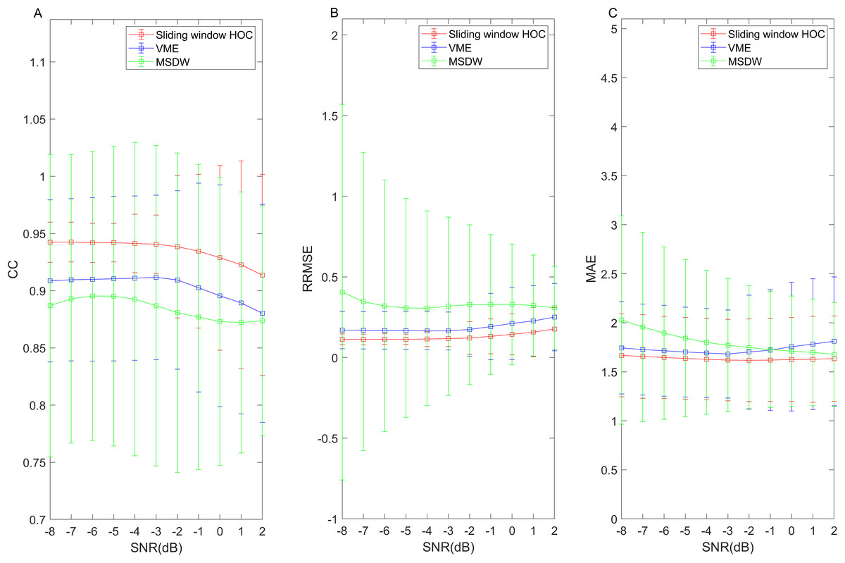
Figure 6: Artifact reduction effectiveness metrics in the semi-simulated data.
Results of metrics measuring the efficacy of artifact reduction (A) CC, (B) RRMSE and (C) MAE based on the sliding window higher-order cumulants (HOCs), variational mode extraction (VME), and multi-window summation of derivatives within a window (MSDW) method. The error bars represent the mean and standard deviation.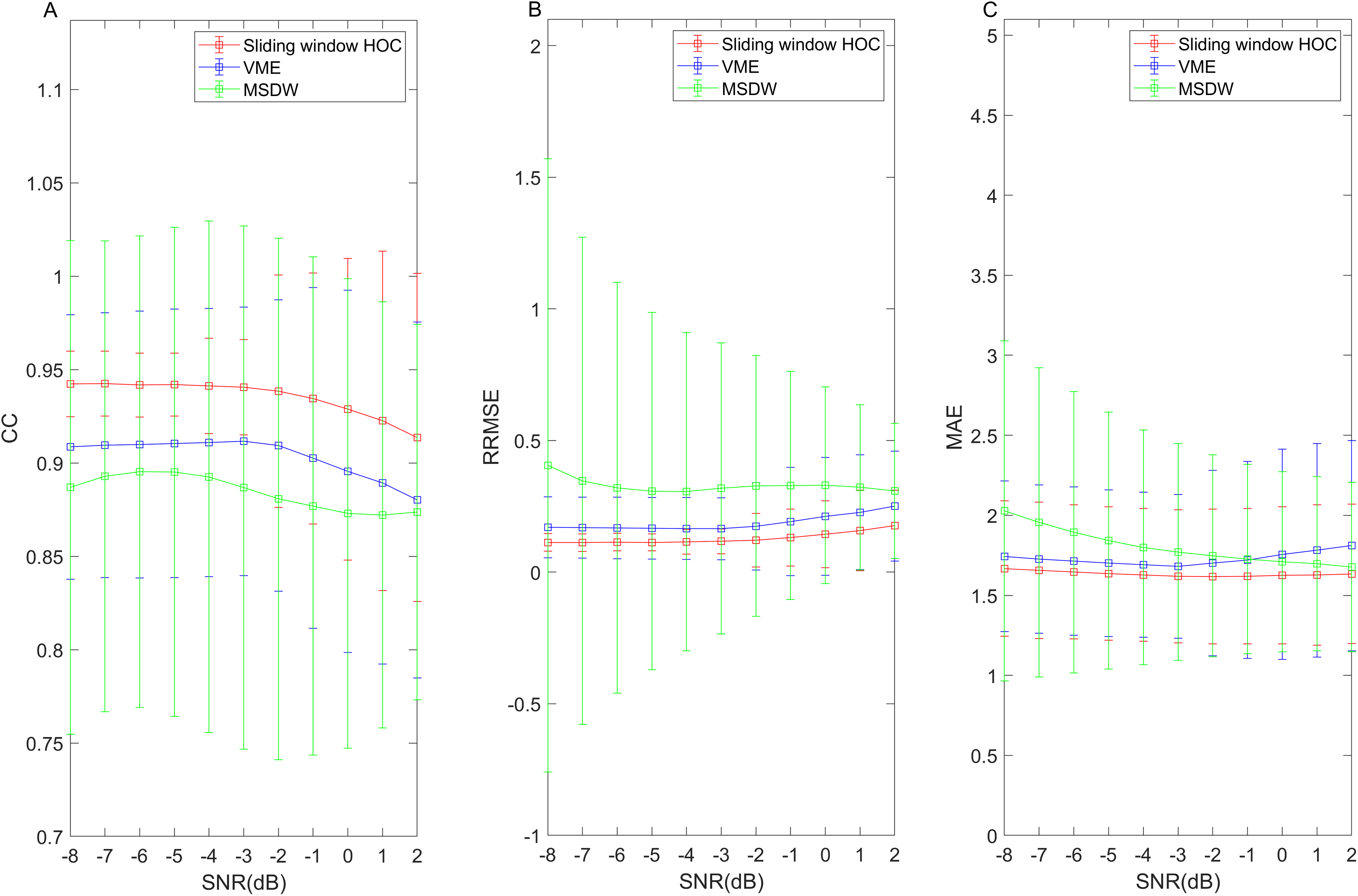
| Detection methods | Sliding window HOCs | VME | MSDW |
|---|---|---|---|
| CC | 0.935 (0.046)a | 0.914 (0.078)b | 0.909 (0.094)c |
| RRMSE | 0.128 (0.077)a | 0.186 (0.234)b | 0.225 (0.414)c |
| MAE | 1.634 (0.424)a | 1.770 (0.670)b | 1.748 (0.574)b |
Note:
Values are presented as mean (std). Groups sharing the same superscript letter are not significantly different (p > 0.05, Bonferroni-corrected), while different letters indicate statistically significant differences.
Results of real data
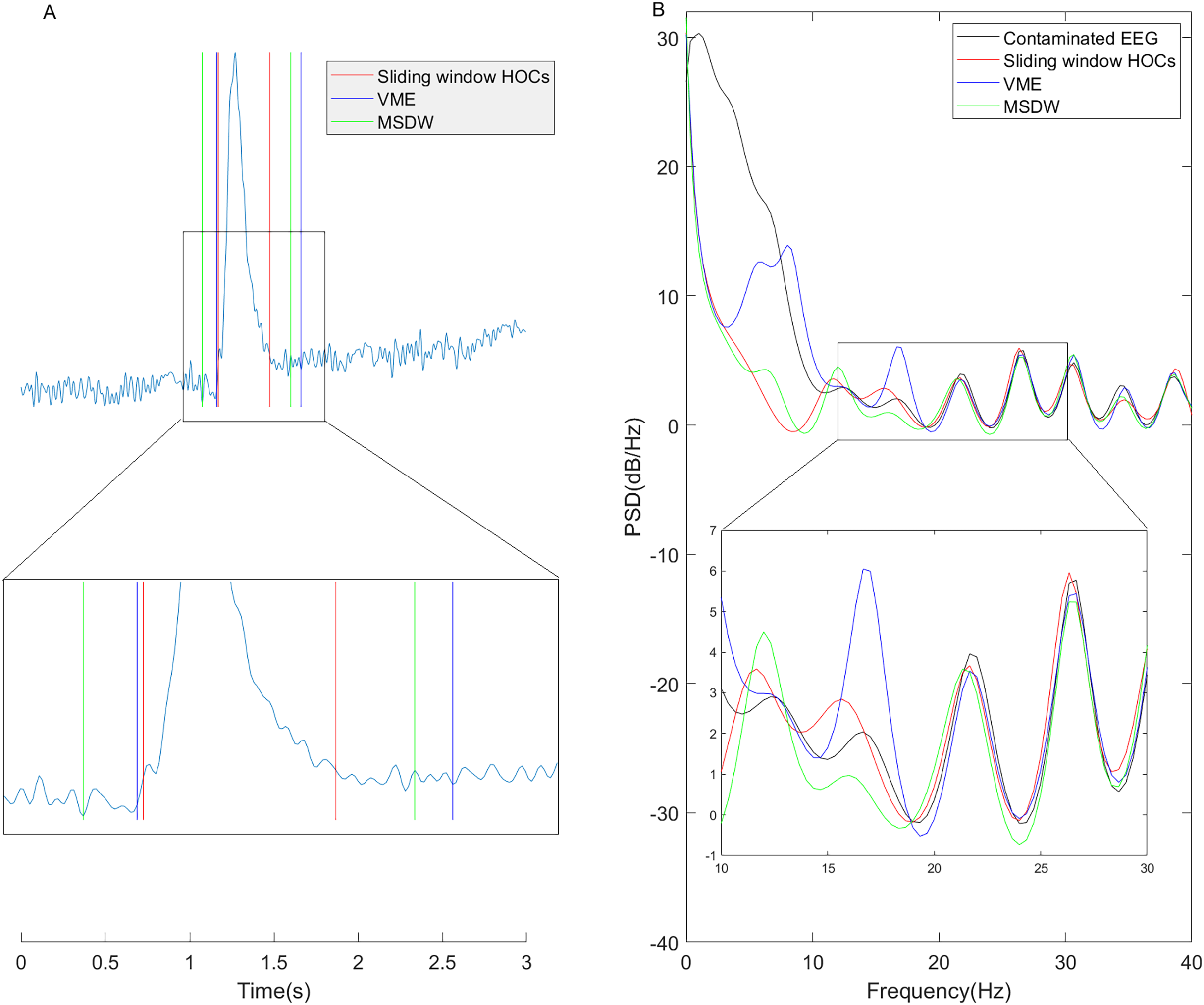
Fig. 7 compares blink artifact detection results in real data using the sliding window HOC, VME, and MSDW methods, alongside power spectra of wavelet-denoised signals following blink detection. Specifically, Fig. 7A demonstrates that the sliding window HOC method more accurately localized artifact occurrence intervals than the other two methods. Figure 7B reveals that the sliding window HOC-based filter achieved improved detection of blink artifacts in the low-frequency range while providing superior signal preservation in the high-frequency range- particularly within the EEG β-band, as shown in the magnified region (Maddirala & Veluvolu, 2021).
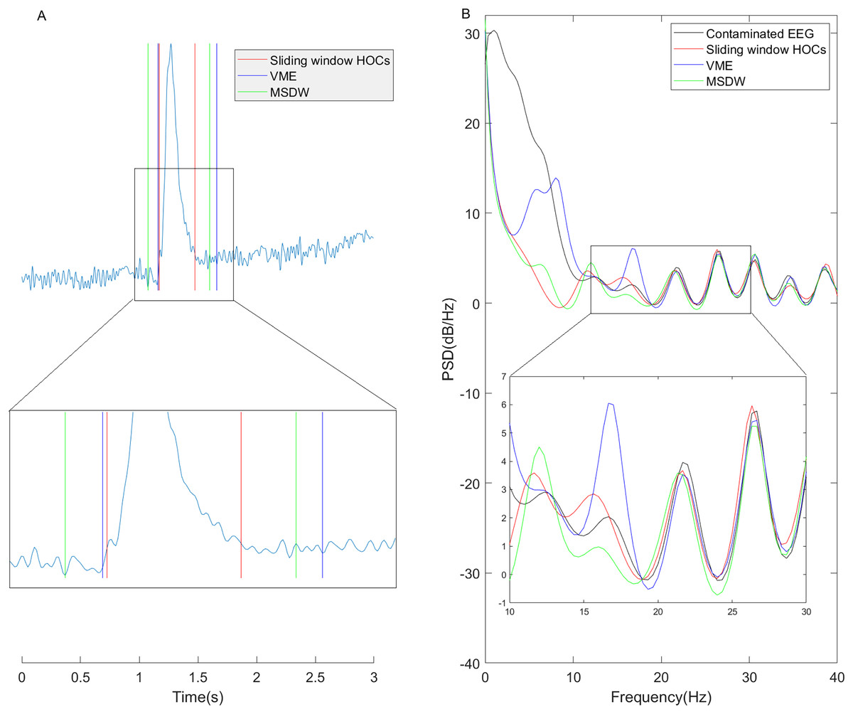
Figure 7: One example of blink artifact detection on a real data segment and the power spectrum of the altered EEG signals based on the detection results.
Figure 8 and Table 4 present box plots of the calculated values across three real datasets. These results confirm that the sliding window HOC-based filter outperformed both the VME and the MSDW methods in attenuating blink artifacts while preserving EEG signals.
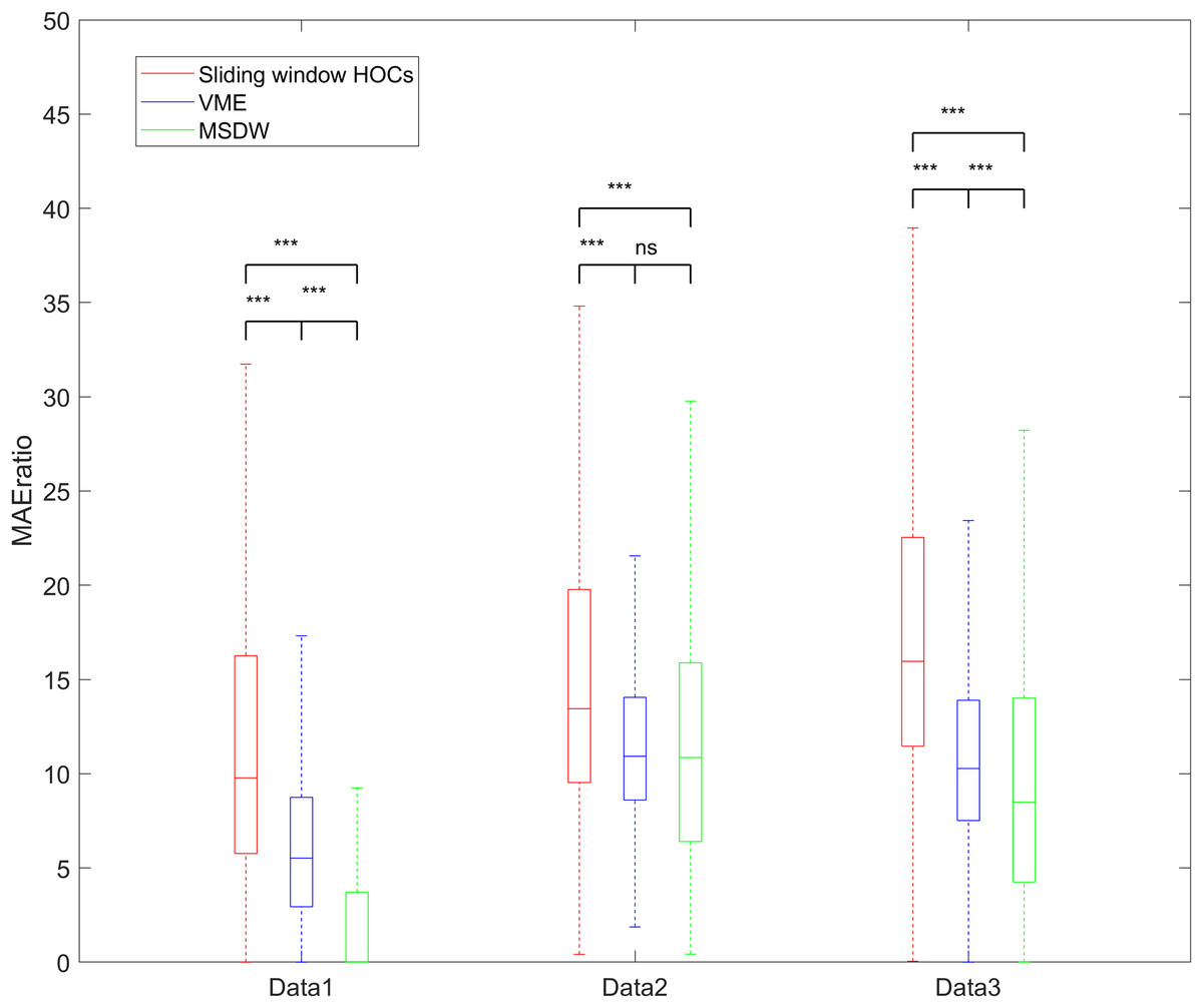
Figure 8: The box chart of the MAEratio of the three datasets.
ns, p > 0.05; ***p < 0.001.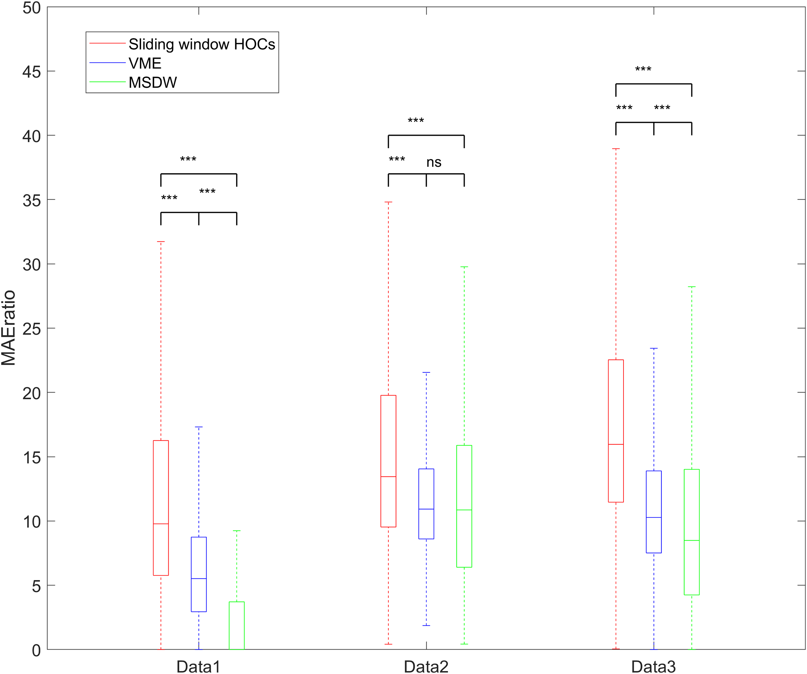
| Datasets | Sliding window HOCs | VME | MSDW |
|---|---|---|---|
| Data1 | 9.785 (10.478)a | 5.523 (5.796)b | 0.000 (3.712)c |
| Data2 | 13.450 (10.223)a | 10.925 (5.431)b | 10.861 (9.427)b |
| Data3 | 15.961 (11.055)a | 10.275 (6.373)b | 8.489 (9.743)c |
Note:
Values are presented as median (interquartile range). Groups sharing the same superscript letter are not significantly different (p > 0.05, Bonferroni-corrected), while different letters indicate statistically significant differences.
Computational time
In single-channel EEG artifact processing, computational efficiency and real-time capability are key evaluation metrics. This study compared the computational efficiency of three blink artifact detection algorithms using semi-simulated and real data. Experiments were conducted in a standardized testing environment: MATLAB 2021b on a hardware with an Intel i7-9700 processor (3.00 GHz base frequency), a 64-bit Windows 10, and 32 GB of RAM. As shown in Table 5, the proposed algorithm demonstrated significantly faster computation than the traditional VME method (Bonferroni-corrected, p < 0.05), though it remained slower than the MSDW algorithm. Our analysis confirmed the sliding window HOC method’s suitability for online, real-time EEG processing applications.
| Data | Sliding window HOCs (s) | VME (s) | MSDW (s) |
|---|---|---|---|
| Semi-simulated data | 0.0052 (0.0013)a | 0.0081 (0.0036)b | 0.0003 (0.0001)c |
| Real data (Data1) | 0.0051 (0.0004)a | 0.0057 (0.0008)b | 0.0003 (0.0001)c |
| Real data (Data2) | 0.0054 (0.0009)a | 0.0066 (0.0014)b | 0.0004 (0.0001)c |
| Real data (Data3) | 0.0056 (0.0009)a | 0.0064 (0.0010)b | 0.0004 (0.0001)c |
Note:
Groups sharing the same superscript letter are not significantly different (p > 0.05, Bonferroni-corrected), while different letters indicate statistically significant differences.
Discussion
This study proposes a sliding window HOC method for detecting artifacts in single-channel EEG. The method’s performance was evaluated using semi-simulated data and real data through direct accuracy metrics and indirect artifact reduction effectiveness metrics. Results demonstrate that: (1) the method can accurately detect blink artifact boundaries in single-channel EEG signals; (2) the method is fully automated as no human involvement is required; and (3) detection leverages the distinct Gaussian characteristics differentiating EEG signals from blink artifacts. In comparison to the VME method, which is limited to positive blink peaks and preset blink intervals, and the MSDW method, which has specific requirements for blink morphology, this method is considered to be more robust.
The sliding window HOC method focuses on accurately identifying blink artifacts. This process not only locates artifacts initially through HOCs, but also precisely determines their start and end positions via further adjustment. While most single-channel EEG blink artifact studies focused on localization (Valderrama, de la Torre & Van Dun, 2018; Shahbakhti et al., 2021a; Maddirala & Veluvolu, 2022a, 2022b), few addressed boundary-specific recognition (Chang et al., 2016). Although the proposed algorithm does not remove blink artifacts, it accurately detects contaminated intervals in single-channel EEG. This capability is essential for future effective artifact removal while preserving the EEG signal.
To improve blink artifact detection accuracy, this study introduces a crucial refinement step- further adjustments to detected blink intervals-following preliminary detection. This step dynamically identifies the precise boundaries of blink artifacts using a dual-threshold system ( and ), overcoming the limitation of fixed-window methods in adapting to variable-duration blinks. To determine the optimal thresholds, a systematic experimental design was employed: 5,940 (108 × 11 × 5) contaminated EEG segments were constructed by varying blink durations (100–500 ms) and SNR levels (–8 to 2 dB). Results demonstrate peak performance at = 0.4 and = 0.2 (Youden index = 0.9422; Fig. 4), significantly improving recognition accuracy across blink characteristics. The further adjustments step enhances the sliding window HOC method, enabling more precise dynamic detection.
The performance of the sliding window HOC method is compared with the VME and MSDW methods. For both semi-simulated data and real data, the results indicate that the sliding window HOC method outperforms both VME and MSDW. This was demonstrated using semi-simulated data generated by mixing blink artifact of varying durations with 377 segments of EEG signals at different SNRs. The sliding window HOC method demonstrates superior performance in direct detection accuracy when compared to other methods. Regarding rough assessment metrics, the sliding window HOC method exhibits the highest Youden index value. While the FPPS of the MSDW algorithm is marginally lower than that of the proposed sliding window HOC method, its is considerably lower than that of the HOC method. Overall, the proposed method is superior to other methods in terms of its capability to localize blink artifacts (see Table 2). In terms of fine assessment metrics, the ROC curves plotted for different combinations of FP and FN tolerances demonstrate that the HOC method has the highest recognition accuracy. This suggests that the HOC method is capable of identifying the boundaries of blink artifacts with the greatest precision (see Fig. 5). Regarding the artifact reduction effect achieved based on the detection methods, the sliding window HOC-based filter shows a higher CC value, lower RRMSE value, and higher MAE (see Fig. 6 and Table 3), indicating better performance in artifact reduction. Despite demonstrating superior performance compared to the other two methods, the detection efficacy of the proposed sliding window HOC method shows a gradual decline as the SNR increases. This phenomenon is characterized by a decline in the CC and an increase in the RRMSE, signifying that variations in SNR have a discernible impact on detection accuracy. This phenomenon is primarily attributable to two factors: Firstly, following the preliminary detection of blink artifact boundaries, the method must accurately localize blink peaks within these boundaries. However, higher SNR levels amplify the influence of blink artifact amplitudes on EEG signals, potentially leading to localization errors during the preliminary detection phase. Secondly, in the subsequent adjustment phase, the method employs these identified blink peaks in conjunction with predefined thresholds, which may reduce the effectiveness of the adjustment. The combined effect of these two factors results in a decline in overall performance in high-SNR environments.
For real data, results from three different databases show that the sliding window HOC-based filter achieves a higher (see Fig. 8 and Table 4), suggesting it is better at attenuating blink artifacts while retaining valid EEG signals. The causes of these results may include: (1) the sliding window HOC method is more accurate in locating the interval boundaries of blink artifacts, resulting in better recognition and filtering effects. (2) the VME and MSDW methods may require further parameter adjustments to improve blink artifact detection. This is particularly true for the VME methods, which fails to recognize blink intervals in many real data fragments; consequently, its is set to 0. This suggests that these algorithms have slightly poorer robustness compared to the sliding window HOC method. Another advantage of the sliding window HOC method is its low CPU time requirement, making it suitable for online and semi-real time applications.
While the proposed sliding window HOC method has been verified to be effective for detecting blink artifacts, several shortcomings require further investigation: (1) The current validation was conducted using specific electrode configurations and recording devices. The method’s performance may vary across different EEG hardware (e.g., dry vs. wet electrodes), montages, or sampling rates. Future studies should evaluate the approach’s robustness across diverse acquisition systems and experimental paradigms. (2) While our validation has demonstrated the method’s efficacy for isolated blink artifact detection, its performance in real-world EEG recordings - which often contain complex mixtures of muscle artifacts, line noise, and various ocular movements - requires further investigation and methodological enhancements. To address these more challenging scenarios, several key developments would be necessary: establishing comprehensive artifact-specific HOC profiles that capture the distinct higher-order statistical signatures of each major contamination type; implementing a hierarchical decision-making framework that intelligently combines multiple discriminative features beyond HOC; and developing robust integration strategies with established artifact handling techniques, such as employing independent component analysis (ICA) for muscle artifact removal and adaptive notch filtering for power line interference suppression. This multi-pronged approach would significantly improve the method’s practical utility in noisy, real-world EEG applications. (3) The two thresholds are determined from semi-simulated data generated by mixing one blink segment (and its duration variations) with 108 pure EEG segments at different SNRs. To enhance universal adaptability, future work should select blink waveforms from a wider range of subjects and recording devices to produce richer semi-simulated data for threshold calibration. (4) The current method can only identify single intervals within short segments; overlapping intervals may be misidentified as a single blink. Parameters for evaluating different blink intervals should be added to enable detection of multiple, separate blink artifacts. (5) This study only detects blink artifacts and does not include the detection of horizontal electrooculograms. Considering the fact that horizontal electrooculograms also have different Gaussian characteristics with EEGs, the sliding window HOC methods can be used to detect horizontal electrooculograms in further work.
Furthermore, our future research will pursue three key directions: First, we will optimize the computational complexity of HOCs to significantly improve processing efficiency while preserving algorithmic advantages, thereby better meeting real-time application requirements. Second, we will develop novel blink artifact removal algorithms. Building upon the high-precision artifact identification method proposed in this study, these algorithms aim to provide a more comprehensive solution to single-channel blink artifact filtering, achieving accurate artifact elimination, preservation of original EEG rhythm power characteristics, and with minimal impact on filtered EEG rhythm power. Third, while this study primarily focuses on single-channel EEG applications, future work will be extended to multi-channel EEG scenarios. By incorporating multi-channel EEG features, we intend to develop targeted solutions for the recognition and filtering of blink artifacts in multi-channel EEG systems. Finally, it should be noted that although this study has demonstrated the superior performance of the sliding-window higher-order cumulant method within the traditional signal processing framework, the rapid advancement and widespread application of deep learning technologies suggest that future research should focus on exploring integration strategies combining higher-order statistical features with deep learning models.
Conclusions
This article proposes the sliding window HOC method for accurately detecting blink artifacts in single-channel EEG. The detection accuracy and general applicability of the method are validated using both semi-simulated and real data. By utilizing the difference in Gaussian characteristics between EEG signals and blink artifact signals, the results from both semi-simulated and real data demonstrate that the proposed sliding window HOC method outperforms VME and MSDW in terms of accuracy metrics and artifact reduction effectiveness metrics. Therefore, this method proves suitable for detecting blink artifacts in single-channel EEG applications.