
Detecting spam and ham SMS messages using natural language processing and machine learning algorithms
- Published
- Accepted
- Received
- Academic Editor
- Giovanni Angiulli
- Subject Areas
- Artificial Intelligence, Data Mining and Machine Learning, Neural Networks
- Keywords
- Classification measures, Ham SMSs, Machine learning, Natural language processing, Spam SMSs
- Copyright
- © 2025 Abdel-Jaber
- Licence
- This is an open access article distributed under the terms of the Creative Commons Attribution License, which permits unrestricted use, distribution, reproduction and adaptation in any medium and for any purpose provided that it is properly attributed. For attribution, the original author(s), title, publication source (PeerJ Computer Science) and either DOI or URL of the article must be cited.
- Cite this article
- 2025. Detecting spam and ham SMS messages using natural language processing and machine learning algorithms. PeerJ Computer Science 11:e3232 https://doi.org/10.7717/peerj-cs.3232
Abstract
Many people use mobile devices for communication, including the short message service (SMS). Attackers can exploit SMS to send spam messages and carry out phishing or malware attacks. These attacks pose risks to users by potentially damaging devices or stealing, altering, or deleting data. The purpose of this study is to detect spam and ham SMSs efficiently. The methodology of this research is to propose a data-driven process model based on natural language processing (NLP) and machine learning algorithms to detect spam and ham SMSs. The machine learning algorithms used in this model are K-nearest neighbors (KNN), decision tree (DT), random forest (RF), gradient boosting (GB), multi-layer perceptron (MLP), and support vector machine (SVM). The proposed model uses several steps, such as deleting punctuation from the dataset, converting data in the dataset into lowercase letters, applying tokenization on the data in the dataset, deleting English stopwords from the dataset, utilizing stemming or lemmatization, using the map function to replace class values with numeric values, using a feature extraction method (CountVectorizer), applying stratified shuffle split cross-validation, using the random oversampling method to solve the imbalanced classes in the dataset, and training and testing the models using the above-mentioned machine learning algorithms. The classification measures used for the considered machine learning algorithms are accuracy, precision, recall, and F1-score. The proposed machine learning models are compared using the classification measures based on balanced or imbalanced dataset to specify which model provides better classification performance. In addition, the proposed machine learning models are compared using the precision-recall curve and the area under the precision-recall curve based on an imbalanced dataset to evaluate the performance of the classification models of the compared algorithms. Moreover, the proposed model is compared with related works to assess its performance against previous works. The experimental results showed that multi-layer perceptron (MLP) offers the highest accuracy, precision, and F1-score results. In addition, KNN, RF, MLP, and SVM provide similar and the highest recall results. Based on the results of the areas under the precision-recall curves, the classification models of the compared algorithms are performing well.
Introduction
Background information
With the rise in mobile device usage and the declining cost of short message service (SMS), the volume of transmitted messages has grown exponentially. SMS is one of the cheapest and most popular communication methods worldwide for exchanging messages between servers (Cormack, 2006). Mobile users send SMS messages for various purposes, including greetings, business communications, and advertisements. This growth has also led to an increase in attackers sending spam SMS messages for malicious purposes (Almeida, Gomez Hidalgo & Yamakami, 2011; Parandeh Motlagh & Khatibi Bardsiri, 2018). Spam SMS messages can be defined as unsolicited SMSs sent without the recipient’s permission (Tekerek, 2017; Sheikhi, Kheirabadi & Bazzazi, 2020; Ahmed et al., 2022; Rajput, Athavale & Mittal, 2019; Alghoul et al., 2018). These messages can contain diverse content, such as promotions, awards, phishing links, or malware, including viruses and Trojans, making them potentially harmful (Mohammadi & Hamidi, 2018; Martin et al., 2005; Rajput, Athavale & Mittal, 2019). For example, a spam SMS might include a phishing link that redirects users to a fraudulent website designed to steal their credentials and, consequently, their financial assets. Spammers often collect users’ contact information from websites, chat rooms, and similar platforms to sell to other spammers, who then use it to send additional spam SMS messages.
Spam filtering systems can be developed using data-driven approaches such as machine learning algorithms (Tekerek, 2017; Sheikhi, Kheirabadi & Bazzazi, 2020; Nyamathulla et al., 2022; Sharma & Arjun, 2023; Moutafis, Andreatos & Stefaneas, 2023; Fatima et al., 2023; Shrivas, Dewangan & Ghosh, 2021; Reddy et al., 2023; Madhavan et al., 2021). Data-driven solutions have demonstrated not only high detection rates but also cost-effectiveness and greater objectivity compared to traditional methods. For instance, Reddy et al. (2023) proposed a natural language processing (NLP) model combined with machine learning algorithms to automatically classify incoming emails as either spam or legitimate.
In Fatima et al. (2023), a machine learning algorithm was proposed to detect spam emails. This algorithm optimizes hyperparameter settings using various parameter optimization methods, including manual search, random search, grid search, and genetic algorithm (GA). Additionally, it incorporates two feature extraction modules: Term frequency-inverse document frequency (TF-IDF) vectorizer and CountVectorizer. The algorithm has been applied to three datasets, one of which is the UCI SMS Spam dataset. The algorithm follows these preprocessing steps: converting all text to lowercase or uppercase, removing hyperlinks, whitespaces, numbers, and punctuation, deleting stopwords, and applying tokenization, stemming, and lemmatization. To detect spam SMS messages, the optimized algorithm employs various machine learning methods. The classification results, such as accuracy, could be further improved by developing a model using machine learning algorithms like random forest (RF) (Breiman, 2001; Cutler, Cutler & Stevens, 2011), multi-layer perceptron (MLP) (Rosenblatt, 1958; Singh & Banerjee, 2019), and support vector machine (SVM) (Cortes & Vapnik, 1995). In Reddy et al. (2023), a project focused on preprocessing using machine learning algorithms and NLP was introduced. This project aimed to provide a system for filtering spam emails. The dataset used consisted of emails classified as either spam or ham. For NLP, preprocessing steps included tokenization, stopword removal, stemming, and feature extraction. The machine learning algorithms employed in this project included naïve Bayes (NB) (Zhang, 2004), SVM, and K-nearest neighbors (KNN) (Cover & Hart, 1967). The accuracy of SVM in this context could be improved by developing a model that combines SVM and NLP techniques, incorporating methods such as punctuation removal, stemming, lemmatization, and advanced techniques like stratified shuffle split cross-validation.
Several studies have proposed models based on machine learning algorithms to detect spam SMS messages, such as the works in Sani, Abdulrahman & Adamu (2025), de Luna et al. (2023), Hossain et al. (2021), Sjarif et al. (2019), GuangJun et al. (2020), Asirvatham & Meenakshi (2025).
Decision tree (DT) (Breiman et al., 1984; Quinlan, 1993; Hastie, Tibshirani & Friedman, 2009), J48 (Frank, Hall & Witten, 2016), and NB algorithms have been compared to detect ham or spam short messages (Sani, Abdulrahman & Adamu, 2025). Two datasets from the UCI repository and ExAIS_SMS were used; the models using k-fold cross-validation were evaluated. Accuracy and area under the receiver operating characteristic curve (AUC-ROC) metrics are used to evaluate the performance of the models. The results showed that the DT achieved the highest accuracy based on the two datasets. NB has accomplished greater ROC-AUC results. The performance of NB and J48 depends on the dataset; both NB and J48 achieve higher accuracy and ROC-AUC results using the UCI dataset. However, they have lower accuracy and ROC-AUC results using the ExAIS_SMS dataset. Moreover, the proposed model in Sani, Abdulrahman & Adamu (2025) and the baseline model have been compared using the accuracy. The results demonstrated that the accuracy of the compared algorithms is higher than that of the baseline model. Therefore, the accuracy results of the compared algorithms are improved. The Nemenyi test can be used to compare different models or classifiers (Hollander, Wolfe & Chicken, 2015). The Nemenyi test P-values are used to show the statistical differences in the rankings of the model (Sani, Abdulrahman & Adamu, 2025). The DT and NB showed no notable differences between them. However, DT and J48 showed observable differences between them.
The SMS spam dataset used in de Luna et al. (2023) was resulted by created three datasets, two of which are from Kaggle, and the researchers obtained the third one. Eleven machine learning algorithms have been compared using accuracy to discover which algorithm provides the highest accuracy in detecting spam or ham SMSs (de Luna et al., 2023). The algorithms used in the comparison are logistic regression (Bisong, 2019), KNN, DT, SVM, RF, Extra Trees (Geurts, Ernst & Wehenkel, 2006), gradient boosting, AdaBoost, XGBoost, Bernoulli naïve Bayes, and Bagging. The results showed that logistic regression provides the highest accuracy result, while KNN provides the smallest accuracy result. The remaining algorithms yield adequate accuracy results. The second, third, and fourth highest accuracy results are achieved by Bernoulli naïve Bayes, RF, and Extra Trees, respectively. The highest four algorithms regarding to accuracy were chosen for optimization. The aim of optimizing these algorithms is to note the influence of optimized parameters on their performance. These optimized algorithms are compared using accuracy, precision, recall, and F1-score to determine which optimized algorithm provides the highest performance results. The results showed that Bernoulli naïve Bayes provides the highest accuracy, recall, and F1-score. RF achieves the second highest accuracy, recall, and F1-score. Logistic regression produces an accuracy higher than Extra Trees. Extra Trees provides higher recall and F1-score than those of logistic regression. In terms of precision, logistic regression provides the highest precision. RF presents the second highest precision. Extra Trees outperforms Bernoulli naïve Bayes in terms of precision. Additionally, the optimized algorithms enhance their accuracy results.
Bernoulli naïve Bayes, Gaussian naïve Bayes, and Multinomial naïve Bayes are compared using TF-IDF and CountVectorizer to determine which algorithm provides the highest accuracy and precision results (de Luna et al., 2023). The results showed that Bernoulli naïve Bayes accomplishes the highest accuracy and precision results using TF-IDF and CountVectorizer. Additionally, the accuracy and precision results of Bernoulli naïve Bayes using TF-IDF are the same as those for Bernoulli naïve Bayes using CountVectorizer. Multinomial naïve Bayes outperforms Gaussian naïve Bayes in terms of accuracy and precision using TF-IDF and CountVectorizer.
The SMS dataset used in Hossain et al. (2021) was taken from Kaggle. SVM and multinomial naïve Bayes algorithms are compared based on three feature extraction processes to determine which algorithm provides the highest accuracy and F1-score results, as well as the lowest computational time in seconds. The three feature extraction processes are pre-processing and TF-IDF, pre-processing and TF-IDF with stemming, and pre-processing, stemming, TF-IDF, and length of the messages. This comparison comprises six experiments, which show the results of accuracy, F1-score, and the computational time based on the three feature extraction processes for the compared algorithms.
The SVM displays the same accuracy and F1-score when the feature extraction process is either pre-processing and TF-IDF or pre-processing and TF-IDF with stemming. However, the computational time for the SVM using pre-processing and TF-IDF with stemming is lower than that of the SVM using pre-processing and TF-IDF. Moreover, SVM produces the smallest accuracy and F1-score results, and the highest computational time when using pre-processing, stemming, TF-IDF, and the Length of the messages.
Multinomial naïve Bayes achieves the highest accuracy using pre-processing and TF-IDF with stemming. Additionally, multinomial naïve Bayes using pre-processing and TF-IDF achieves higher accuracy than multinomial naïve Bayes using pre-processing, stemming, TF-IDF, and Length of the messages. Multinomial naïve Bayes using pre-processing and TF-IDF has the lowest computational time. Moreover, multinomial naïve Bayes using pre-processing and TF-IDF with stemming has lower computational time than multinomial naïve Bayes using pre-processing, stemming, TF-IDF, and length of the messages. Multinomial naïve Bayes accomplishes the same F1-score using any given feature extraction process.
Multinomial naïve Bayes outperforms the SVM in terms of accuracy, regardless of the feature extraction process used. In addition, the computational times of multinomial naïve Bayes are less than those of SVM using any given feature extraction method. Both Multinomial naïve Bayes and SVM achieve the same F1-score when either pre-processing and TF-IDF or pre-processing and TF-IDF with stemming is used. Multinomial naïve Bayes achieves a higher F1-score than the SVM when pre-processing, stemming, TF-IDF, and length of the messages are applied.
Multinomial naïve Bayes outperforms SVM in terms of the micro average area under the ROC curve (Hossain et al., 2021). As a result, Multinomial naïve Bayes can detect spam SMSs based on stemming and TF-IDF better than SVM.
In Hossain et al. (2021), another comparison has been conducted among Bernoulli naïve Bayes and the works in Sjarif et al. (2019) and GuangJun et al. (2020). The work in Sjarif et al. (2019) employed the RF algorithm, while the work in GuangJun et al. (2020) utilized the logistic regression algorithm. The compared algorithms use TF-IDF feature extraction. This comparison is based on accuracy and F1-score. The results showed that Bernoulli naïve Bayes outperforms both RF and logistic regression in terms of accuracy and F1-score. Additionally, logistic regression provides higher accuracy and F1-score results than RF.
Different machine learning algorithms have been compared based on accuracy, precision, recall, and F1-score to determine which algorithm offers higher performance in detecting spam or ham SMSs (Asirvatham & Meenakshi, 2025). The compared algorithms are linear regression, logistic regression, KNN, NB, and SpamSMS. The results demonstrated that SpamSMS provides the highest accuracy. Both SpamSMS and logistic regression offer the same and the highest precision result. SpamSMS and NB produce the same and the highest recall result. NB provides the highest F1-score.
Motivations
The primary motivations for this research are as follows:
The potential theft of personal credentials through spam SMS messages.
The consumption of mobile device resources caused by spam SMS messages.
The disruption caused by the receipt of unwanted SMS messages, particularly spam.
Problem statement
SMS messages are a popular way of communicating between people. Spam SMSs are undesired messages because they may contain advertisements, malicious links, and other content that can harm people. Spam SMSs can also affect the security and privacy of people. Cybercriminals can use malicious links in spam SMS messages to commit cybercrimes, such as downloading malware, stealing user information, or redirecting users to phishing websites. Cybercriminals use spam SMSs to commit deceptive operations, such as stealing users’ financial assets. The device’s resources can be largely consumed when many spam SMSs are received, such as the device’s storage. As a result, the performance of networks is influenced. The recipient of SMSs spends more time filtering SMSs to specify whether an SMS is spam or ham.
The problems of this research are as follows:
Cybercriminals can send spam SMSs that convey undesirable content to recipients, such as advertisements.
Spam SMSs can be used to commit fraud, such as illegally obtaining users’ credentials and money.
Spam SMS can contain malware that can be used to attack users’ devices and data.
Using memory space in storing spam SMSs.
Spending more time dealing with spam SMSs by users.
Research questions
The research questions addressed in this work are as follows:
How can spam and ham SMS messages be detected?
How can users’ information be secured?
How can mobile device resources be preserved?
Which machine learning algorithm among those compared is most effective in detecting spam SMS messages?
Which algorithm offers the best classification results among the compared models?
Aims
Detecting spam SMS messages is crucial for achieving several aims, including but not limited to:
Securing user information
Protecting mobile devices
Saving user time and resources
Preserving device resources
These aims can be accomplished through the use of spam filter systems.
Main contributions
The main contributions of this research are as follows:
The novel contribution is developing a data-driven process, which contributes to proposing a model based on machine learning algorithms and NLP.
Proposing a data-driven model based on NLP and machine learning algorithms to detect spam and ham SMS messages. This model classifies SMS messages as either spam or ham, functioning as a spam filter system. It can block spam SMS messages and allow legitimate ham SMS messages to reach their recipients, contributing to the protection of users’ information, finances, and devices.
Evaluating the performance of the proposed model using several machine learning algorithms, balanced dataset, and different evaluation metrics, such as accuracy, precision, recall, and F1-score. This evaluation helps determine which machine learning model provides the best classification performance, making it suitable for use as a detection system for spam and ham SMS messages.
Evaluating the performance of the proposed model using several machine learning algorithms, an imbalanced dataset, and the abovementioned evaluation metrics, the precision-recall curve, and the area under the precision-recall curve. This evaluation helps determine which machine learning model provides the best classification performance, making it suitable for use as a detection system for spam and ham SMS messages. Additionally, evaluating the performance of classification models of the compared algorithms based on the precision-recall curve and the area under the precision-recall curve.
Comparing the results of the proposed model with those of previously published works to create a benchmark for future research in spam and ham SMS detection. This comparison also evaluates the performance of the proposed model against prior methods, helping to establish the superiority of the model based on classification metrics.
Organization of the article
The remainder of this article is organized as follows. ‘Related Works’ presents the related works, ‘The Proposed Model’ details the proposed model, ‘Discussions’ discusses the findings, and ‘Conclusions’ concludes the article.
Related works
Many studies have been conducted on spam detection in SMS messages. This section reviews related works on spam detection in SMS using data-driven techniques, focusing particularly on machine learning algorithms.
In Tekerek (2017), several machine learning techniques for detecting SMS spam were compared, including KNN, RF, NB, SVM, and RT (Gupta, Mohan & Shidnal, 2018; Kalmegh, 2015). The authors used the SMS Spam Collection dataset (Almeida, Gomez Hidalgo & Yamakami, 2011), which includes 4,827 ham SMS messages and 747 spam SMS messages. A 10-fold cross-validation method was employed during the training and testing of the machine learning algorithms. The study found that SVM achieved the highest predictive accuracy of 98.33%, with a false positive rate of 0.087.
In Sheikhi, Kheirabadi & Bazzazi (2020), a machine learning algorithm for detecting SMS spam was proposed. This method is divided into two key stages: feature extraction and decision making. To reduce complexity and improve model performance, the feature extraction stage focuses on identifying features based on the characteristics of spam and legitimate messages. An average neural network model is then applied to these features to classify messages as either spam or legitimate. The dataset used in this study is from the UCI machine learning repository (Dua & Graff, 2017), which contains 4,827 ham messages and 747 spam messages.
In Nyamathulla et al. (2022), the authors studied spam detection using several machine learning algorithms on the same UCI dataset (Dua & Graff, 2017). They employed KNN, DT (Breiman et al., 1984; Quinlan, 1993; Hastie, Tibshirani & Friedman, 2009), RF, NB, and SVM algorithms to assess their effectiveness in detecting spam messages. The data preparation involved constructing a sparse matrix by removing digits, punctuation, stopwords, and blank spaces from the SMS messages. The dataset was split into 75% for training and 25% for testing. Experimental results were based on CountVectorizer with an imbalanced dataset, CountVectorizer with the synthetic minority oversampling technique (SMOTE) for balancing the dataset, TF-IDF, and hashing vectorizer. The study also compared the results to other published works, such as a deep learning-based long short-term memory (LSTM) model (Hochreiter & Schmidhuber, 1997), RF (Amir Sjarif, Mohd Azmi & Chuprat, 2019), and SVM (Navaney, Dubey & Rana, 2018), with the proposed method showing higher predictive accuracy than those reported in Amir Sjarif, Mohd Azmi & Chuprat (2019) and Navaney, Dubey & Rana (2018).
In Sharma & Arjun (2023), the authors compared various classification algorithms, including NB (multinomial and Bernoulli), KNN, DT, logistic regression (Bisong, 2019), RF, bagging (Breiman, 1996), Extra Trees (Geurts, Ernst & Wehenkel, 2006), and XGBoost (Chen & Guestrin, 2016), using the spam dataset from Kaggle (2025). The dataset consists of 5,572 instances and four attributes, with 672 spam messages and 4,900 ham messages. The study found that DT and NB produced the best accuracy results.
Moutafis, Andreatos & Stefaneas (2023) investigated spam message detection using several machine learning algorithms, including SVM, KNN, NB, neural networks (Rumelhart, Hinton & Williams, 1986; Grosan & Abraham, 2011), RNNs (Marhon, Cameron & Kremer, 2013), AdaBoost (Mazini, Shirazi & Mahdavi, 2019), RF, GB (Hastie, Tibshirani & Friedman, 2009; Friedman, 2001), logistic regression (Bisong, 2019), and DT. The authors used the SpamAssassin dataset, consisting of 501 spam and 2,551 ham emails (https://www.kaggle.com/code/sergiovirahonda/spamassasin-spam-exploration-prediction/notebook?scriptVersionId=38100646), as well as the Enron 1 dataset, which includes 3,219 spam and 3,228 ham emails (https://www2.aueb.gr/users/ion/data/enron-spam), and a CSV file provided by Faisal Qureshi (Kaggle, 2022).
In Fatima et al. (2023), an algorithm was proposed that optimizes hyperparameter tuning for detecting spam emails. The parameter optimization methods considered were manual search, random search, grid search, and GA. Two feature extraction modules were used: TF-IDF vectorizer and CountVectorizer. These modules were applied to three datasets: Ling Spam (2,893 emails, with 481 spam and 2,412 ham) (Kaggle, 2019a), UCI SMS Spam (5,574 emails, with 747 spam and 4,827 ham) (Dua & Graff, 2017), and a dataset with 6,510 emails (1,678 spam and 4,832 ham). Several machine learning algorithms were used to measure classifier performance, including NB, SVM, RF, MLP, logistic regression, extra tree (Geurts, Ernst & Wehenkel, 2006), and stochastic gradient descent (SGD) (Bottou, 2010).
Reddy et al. (2023) presented a project based on machine learning algorithms and NLP to classify emails. The goal was to develop a spam filter system capable of accurately classifying spam emails. The dataset used contained a large number of email messages with their corresponding spam or ham labels. NLP methods such as tokenization, stopword removal, and stemming were employed for data preprocessing, and feature extraction was performed. Machine learning algorithms, including NB and SVM, were tested to determine the best model for classifying emails. Hyperparameter tuning was applied to optimize the model’s performance. Empirical results demonstrated that KNN, NB, and SVM algorithms achieved accuracies above 90%.
In Madhavan et al. (2021), the authors compared several machine learning algorithms (KNN, SVM, NB, and rough sets (Pawlak, 1982; Pérez-Díaz et al., 2012)) for spam email detection. They used various evaluation measures, such as accuracy, precision, and recall, to assess the performance of the models derived from these algorithms. The results showed that KNN, SVM, NB, and rough sets classifiers all achieved high predictive accuracy, exceeding 90%.
Shrivas, Dewangan & Ghosh (2021) compared several machine learning algorithms (NB, RF, J48 (Yadav & Chandel, 2015), RT, and AdaBoost (Mazini, Shirazi & Mahdavi, 2019)) for detecting spam emails. The authors used six different versions of the Enron dataset and created a new combined Enron dataset by merging these six datasets. During data preparation, irrelevant words were removed using techniques such as word counting, stemming, tokenization, pruning, and stopword removal. A 10-fold cross-validation was applied.
Feature selection methods such as ReliefF (Yang et al., 2011), information gain (IG) (Lei, 2012), chi-square (Rachburee & Punlumjeak, 2015), and SymmetricalUncert (Dai et al., 2020) were used, followed by a ranker approach in the combined dataset for the RF algorithm. The confusion matrix was computed for all RF datasets, and performance measures such as accuracy, precision, specificity, F-measures, false positive rate (FPR), and true positive rate (TPR) were used. The results indicated that SymmetricalUncert provided the best results for accuracy, precision, specificity, and F-measures, while chi-square produced the largest TPR. A comparison of the RF classifier with other machine learning classifiers showed that RF achieved the highest accuracy across all seven Enron datasets.
The details of the related works are summarized in Table 1, including the year of publication, machine learning methods used, datasets, dataset sizes, data preparation methods, evaluation methods, and citations.
| Year of publication | Machine learning methods used | Datasets used | Dataset sizes | Data preparation methods used | Evaluation methods used | Citation no. |
|---|---|---|---|---|---|---|
| 2017 | KNN, RF, NB, SVM, and RT. | SMS spam collection (Almeida, Gomez Hidalgo & Yamakami, 2011; Dua & Graff, 2017). | 4,827 ham SMSs and 747 spam SMSs. | 10-fold cross-validation. | Success rate and false positive rate. | Tekerek (2017) |
| 2020 | The proposed model, RT, NB, J48, decision stump (Iba & Langley, 1992), Hoeffding tree (Hulten, Spencer & Domingos, 2001), SVM, random forest, H2O + random forest (Suleiman & Al-Naymat, 2017). | SMS spam collection (Dua & Graff, 2017). | 4,827 ham SMSs and 747 spam SMSs. | Feature extraction (first stage) and decision making (second stage). | Accuracy, precision, recall, and F1-score. | Sheikhi, Kheirabadi & Bazzazi (2020) |
| 2022 | NB, SVM, and the maximum entropy; logistic regression, KNN, DT, RF; moreover, long short-term memory (LSTM). | SMS spam collection (Dua & Graff, 2017). | 4,827 ham SMSs and 747 spam SMSs. | A sparse matrix is created after removing digits, punctuation marks, stopwords, and blank spaces from SMS messages. The dataset is split into 75% for training and 25% for testing. Additional techniques include using CountVectorizer on an imbalanced dataset, applying the synthetic minority oversampling technique (SMOTE) for balancing, and using TF-IDF and hashing vectorizer. | Accuracy, precision, and recall. | Nyamathulla et al. (2022) |
| 2023 | NB-based multinomial and Bernoulli, KNN, DT, logistic regression, RF, bagging, extra trees, XGBoost. | Spam dataset on Kaggle (2025). | 5,572 instances: 672 spam emails and 4,900 ham emails, with 4 attributes. | Clean the dataset by deleting undesired data, renaming variables, labeling spam and ham messages, repairing missing data, removing duplicates, and appending extra features (e.g., letter count, word count, sentence count). | Accuracy, confusion matrix, and precision. | Sharma & Arjun (2023) |
| 2023 | SVM, KNN, NB, neural networks (Grosan & Abraham, 2011), recurrent neural networks (Marhon, Cameron & Kremer, 2013), AdaBoost (Mazini, Shirazi & Mahdavi, 2019), RF, GB (Hastie, Tibshirani & Friedman, 2009; Friedman, 2001), logistic regression (Bisong, 2019), and DT. | SpamAssasin (https://www.kaggle.com/code/sergiovirahonda/spamassasin-spam-exploration-prediction/notebook?scriptVersionId=38100646), Enron 1 (https://www2.aueb.gr/users/ion/data/enron-spam), and a csv data file (spam.csv) provided by Faisal Qureshi (Kaggle, 2022). | SpamAssassin dataset: 501 spam emails and 2,551 ham emails. Enron 1 dataset: 3,219 spam emails and 3,228 ham emails. Additional dataset (spam.csv): 5,572 messages, 13% spam, and 87% ham. 5,157 unique values. | The dataset is split with 75% for training and 25% for testing, with CountVectorizer used for feature extraction. | Accuracy, with a CSV file providing source IP addresses of spam emails, origin countries, geographical locations of spammers, and graphical and textual statistics. | Moutafis, Andreatos & Stefaneas (2023) |
| 2023 | NB, SVM, RF, MLP, logistic regression, extra tree (Geurts, Ernst & Wehenkel, 2006), and stochastic gradient descent (SGD) (Bottou, 2010). | Ling spam (Kaggle, 2019b), UCI SMS spam (Dua & Graff, 2017), and (Fatima et al., 2023) dataset. | Ling Spam dataset: 2,893 emails (481 spam, 2,412 ham); UCI SMS Spam dataset: 5,574 emails (747 spam, 4,827 ham); additional dataset: 6,510 emails (1,678 spam, 4,832 ham). | Hyperparameter optimization methods such as manual search, random search, grid search, and genetic algorithm (GA) are employed. Two feature extraction methods, TF-IDF vectorizer and CountVectorizer, are used. | Accuracy, macro average precision, macro average recall, and macro average F1-score. | Fatima et al. (2023) |
| 2021 | NB, RF, J48 (Yadav & Chandel, 2015), RT, and AdaBoosting (Mazini, Shirazi & Mahdavi, 2019). | Six different versions of the Enron dataset were used, along with a combined dataset created by merging these six versions. | Enron-1: 3,671 ham, 1,500 spam; Enron-2: 4,361 ham, 1,496 spam; Enron-3: 4,012 ham, 1,500 spam; Enron-4: 1,500 ham, 4,499 spam; Enron-5: 1,500 ham, 3,675 spam; Enron-6: 1,500 ham, 4,500 spam. Combined Enron dataset: 16,383 ham, 16,383 spam. |
Data preparation includes counting words, stemming, tokenization, pruning, and stopwords removal. 10-fold cross-validation is performed. Feature selection methods such as ReliefF, information gain (IG), chi-square, and SymmetricalUncert are applied, followed by the ranker approach in the combined dataset for the RF algorithm. | Accuracy, confusion matrix, true positive rate (TPR), false positive rate (FPR), precision, specificity, and F-measures. | Shrivas, Dewangan & Ghosh (2021) |
| 2023 | KNN, NB, and SVM. | A dataset of email messages, each labeled as either spam or ham. | A large dataset of email messages labeled as spam or ham. | Tokenization, stopwords removal, stemming, and feature extraction are applied. Hyperparameter tuning is conducted. | Accuracy. | Reddy et al. (2023) |
| 2021 | KNN, SVM, NB, and rough sets (Pawlak, 1982; Pérez-Díaz et al., 2012). | Dataset of emails (corpus). | A corpus of emails consisting of spam and non-spam messages. | Null, duplicate, and missing values are removed. The dataset is split into training and testing sets. | Accuracy, spam precision, and spam recall. | Madhavan et al. (2021) |
The related works have several research gaps. Not all steps of the proposed data-driven process model, based on NLP and machine learning algorithms, are applied in previous studies. Additionally, some works did not use all the evaluation metrics employed by the proposed model. Furthermore, certain studies could benefit from improvements in classification metrics, such as recall and F1-score.
Comparison of the proposed model and related works
Tables 1 and 2 can be used to compare the proposed model with the related works based on the datasets used, dataset sizes, data preparation methods, and evaluation methods.
| Machine learning methods used | Dataset used | Dataset size | Data preparation methods used | Evaluation methods used |
|---|---|---|---|---|
| KNN, DT, RF, GB, MLP, and SVM. | SMS Spam Collection (Kaggle, 2023). | 4,825 ham SMSs and 747 spam SMSs. | Removing punctuation marks from SMS messages, converting the text to lowercase, performing tokenization, removing English stopwords, applying stemming or lemmatization, using CountVectorizer for feature extraction, applying stratified shuffle split cross-validation, and employing random oversampling for handling class imbalance. | Accuracy, precision, recall, and F1-measure. |
An overview of the similarities and differences between the proposed model and the related works is presented below:
The model in Nyamathulla et al. (2022) employed methods not used in the proposed model, including NB, maximum entropy, logistic regression, and LSTM. Conversely, the proposed model uses GB and MLP, which are not part of the model in Nyamathulla et al. (2022).
The models in Nyamathulla et al. (2022), Moutafis, Andreatos & Stefaneas (2023) used 75% of the dataset for training and 25% for testing, while the proposed model uses stratified shuffle split cross-validation.
The technique in Sheikhi, Kheirabadi & Bazzazi (2020) incorporates the methods used in the proposed model, along with additional techniques such as RT, NB, J48, decision stump, Hoeffding tree, SVM, and H2O + RF. The technique in Shrivas, Dewangan & Ghosh (2021) uses NB, RF, J48, RT, and AdaBoosting. The technique in Sharma & Arjun (2023) includes NB-based multinomial and Bernoulli, KNN, DTs, logistic regression, RF, bagging, extra trees, and XGBoost. The proposed model in this study uses KNN, DT, RF, GB, MLP, and SVM.
DT, RF, GB, and MLP are used in the proposed model but are not part of the techniques in Reddy et al. (2023), Madhavan et al. (2021). In addition, the technique in Reddy et al. (2023) uses only accuracy as the performance measure, while the technique in Madhavan et al. (2021) uses accuracy, spam precision, and spam recall. The technique in Sharma & Arjun (2023) uses accuracy, confusion matrix, and precision, while the proposed model uses accuracy, precision, recall, and F1-score. Stemming and lemmatization are employed in the proposed model, while only stemming is used in the techniques in Shrivas, Dewangan & Ghosh (2021), Pawlak (1982)
The differences between the optimized algorithm (Fatima et al., 2023) and the proposed algorithm are as follows:
The dataset of the optimized algorithm is split into 80% for the training set and 20% for the testing set. In contrast, the proposed algorithm splits the dataset using stratified shuffle split cross-validation, which divides the dataset into ten randomized splits, maintaining the percentage of samples for each class target as in the entire dataset. Additionally, the optimized algorithm uses both TF-IDF vectorizer and CountVectorizer modules for feature extraction, while the proposed algorithm uses only the CountVectorizer module. The optimized algorithm employs parameter optimization techniques to set the parameters to their optimal values, whereas these approaches are not applied in the proposed algorithm. The optimized algorithm converts letters to both upper and lower case, whereas the proposed algorithm converts all letters to lower case. The optimized algorithm removes numbers, white spaces, and hyperlinks, while the proposed algorithm does not remove these elements. Moreover, the optimized algorithm does not address the imbalanced dataset issue, while the proposed algorithm handles it using the random oversampling method.
The differences between the technique in Tekerek (2017) and the proposed algorithm are as follows: the technique uses 4,827 ham SMS messages, while the proposed algorithm uses 4,825 SMS messages. The technique uses 10-fold cross-validation, while the proposed algorithm uses stratified shuffle split cross-validation, which provides randomized splits, ensuring that the percentage of samples for each class label remains the same as in the entire dataset. The technique does not include several NLP steps, such as removing punctuation, converting SMS messages to lowercase letters, deleting stopwords, or using stemming and/or lemmatization. In contrast, the proposed algorithm applies all of these NLP steps. In the technique, the features are automatically generated from the dataset, whereas the proposed algorithm uses CountVectorizer for feature extraction. Additionally, the technique does not address the issue of an imbalanced dataset, as there are more ham SMS messages than spam SMS messages. On the other hand, the proposed algorithm tackles this issue by balancing the dataset.
The proposed model
The proposed model is executed in several steps:
Obtaining the dataset
Removing punctuation from the dataset
Converting all text to lowercase
Tokenizing the data to obtain tokens
Removing English stopwords
Applying either stemming or lemmatization
Applying the map function to replace class values with numeric values: spam with 0 and ham with 1
Using CountVectorizer for feature extraction
Applying stratified shuffle split cross-validation, which splits the dataset into ten randomized splits (Number of folds), ensuring each split maintains the same proportion of samples from every class label as in the entire dataset (stratification method). The random_state parameter is set to an integer value that is 42 for reproducible result through several function calls (Pedregosa et al., 2011).
Using random oversampling to address class imbalance
Training and testing machine learning models to obtain classification metrics: accuracy, precision, recall, and F1-score
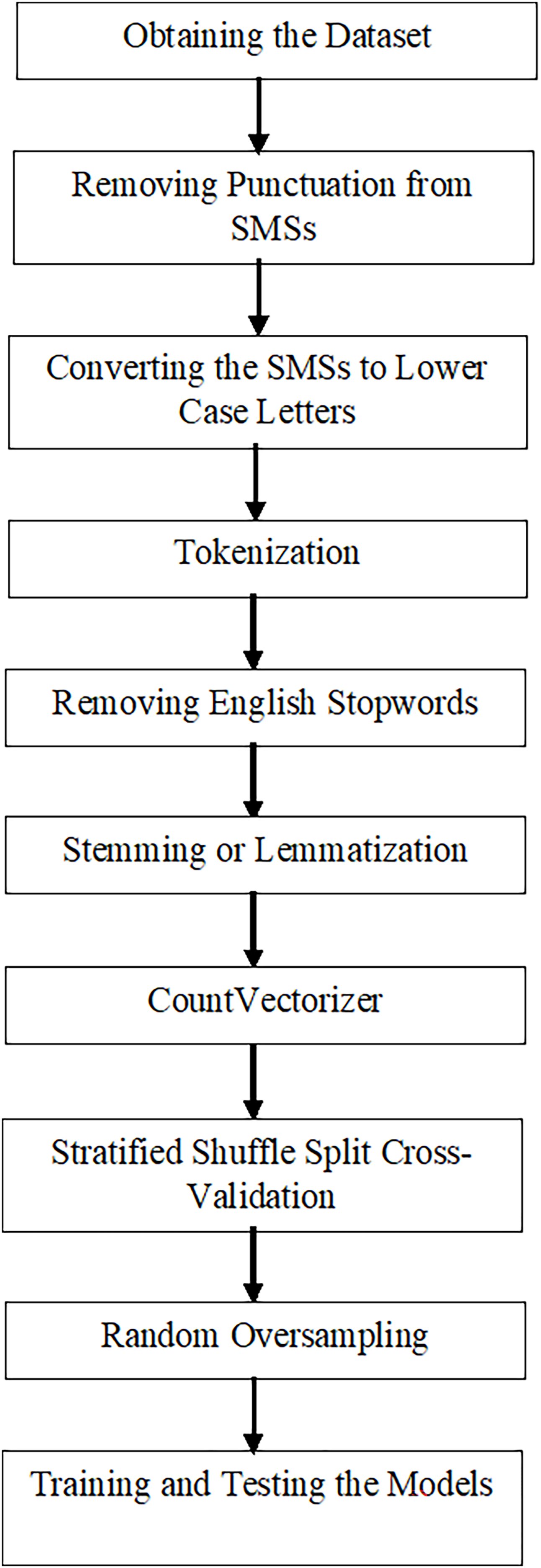
The SMS Spam Collection dataset is sourced from Kaggle. The dataset undergoes preprocessing to clean and prepare the SMSs for analysis. Punctuation marks are removed as they do not add meaningful value, and the text is converted to lowercase for consistency. Tokenization is applied to break the SMSs into smaller units, or tokens, which are useful for analysis. English stopwords are removed, as these are high-frequency words that do not contribute significantly to the meaning of the dataset. Stemming and lemmatization are applied to reduce words to their base forms. Stemming involves trimming letters from the end of words to produce stems, while lemmatization converts words into their lemma, or base form. The map function relaces spam with 0 and ham with 1. For feature extraction, CountVectorizer is employed to transform the SMSs into a matrix where the columns represent tokens, the rows represent SMSs, and each cell contains the count of a token’s occurrence in an SMS. CountVectorizer is used because it has several advantages (Van Otten, 2023), such as the simplicity of CountVectorizer, which means CountVectorizer is simple, easy to understand, and use. In addition, CountVectorizer owns particular parameters and demands low configuration to begin with the processing of text. The second advantage is that CountVectorizer is fast and efficient, which means CountVectorizer is efficient in computation and can process datasets with significant texts and many documents. CountVectorizer uses representations of sparse matrix that save processing time and memory, particularly when treating data with high dimensions. The third advantage is versatility, which means CountVectorizer permits elastic tokenization selections. Moreover, CountVectorizer controls the vocabulary size and allows filtering of the stop words. The fourth advantage is that CountVectorizer provides interpretable results, which means the resulted matrix offers interpretable results, where each cell has a value that represents the count of a token in a particular document, permitting direct exploration and analysis.
The models of transformers have several limitations (AIML.com, 2023), such as the requirements of large computations, large memory, and large training times. In addition, there is an enormous complexity of transformer-based models’ architectures. This leads to the difficulty of interpreting them. The big models are computationally intensive and energy intensive. Considerations of ethics and bias, which means training upon big available data, the language models can, without intention, inherit biases provided in the data. As a result, biased results are presented. The transformer models such as Bidirectional Encoder Representations from Transformers (BERT), DistilBERT, and RoBERTa encounter a limitation: the length of content (Bambroo & Awasthi, 2021). The model size is another limitation (Bambroo & Awasthi, 2021). As a result, these two limitations can limit the performance of transformer models (Bambroo & Awasthi, 2021).
Convolutional neural network (CNN) has different limitations (Smith, 2025), such as inadequate dealing with sequential data. Inadequate treatment for time-series data. Request massive datasets for efficient learning. LSTM has dissimilar limitations (Smith, 2025), such as complex gating methods, which results in computationally expensive. LSTM has slower training times than either CNN or transformers.
Stratified shuffle split cross-validation is used to divide the dataset into ten randomized splits, ensuring each class label is proportionally represented in each split. To address class imbalance, random oversampling is applied, where spam samples are randomly duplicated until the number of spam messages equals the number of ham messages. Finally, machine learning models are trained and tested to evaluate the classification results, including accuracy, precision, recall, and F1-score.
Further details on these steps can be found in ‘The Dataset’–‘Training and Testing the Models’.
The structure of the proposed model is illustrated in Fig. 1.
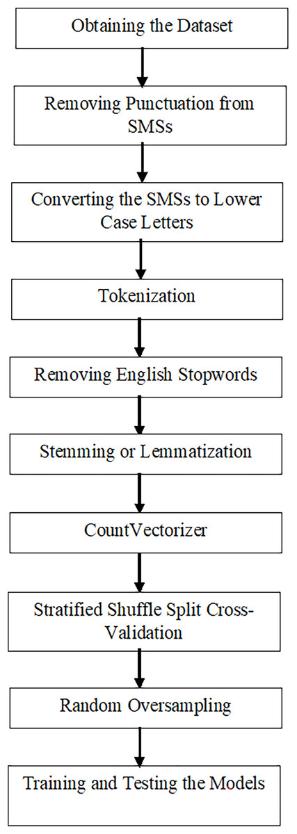
Figure 1: Structure of the proposed model.
The dataset
The SMS Spam Collection dataset, available on Kaggle (2023) and also referenced in Dua & Graff (2017), is used in this study. The dataset contains two columns: the first column represents the labels, and the second contains the SMS messages. The labels are divided into two classes: spam and ham. “Spam” refers to unwanted or unsolicited electronic messages, while "ham" refers to non-spam messages. This dataset consists of 5,572 SMS messages, with 747 messages classified as spam and 4,825 messages classified as ham. This creates an imbalanced dataset, with a significant disparity between the number of spam and ham messages. The minority class is spam, and the majority class is ham. The dataset was selected based on the following criteria: it is relevant to the problem of detecting spam SMS messages, as it includes both spam and ham SMSs. It has a sufficient size, offering a variety of both types of messages. Additionally, the dataset is sourced from Kaggle, a reliable platform, ensuring its credibility for research purposes.
Preprocessing methods of the data
This subsection outlines the data preparation and cleaning steps applied in this study. NLP methods are utilized to prepare and clean the data. NLP, a subfield of artificial intelligence (AI), enables computers to understand human languages (Khurana et al., 2023). One of the key applications of NLP is text classification. In this article, the following NLP methods are applied to preprocess the data:
Punctuation marks are removed from the SMS messages.
All SMS messages are converted to lowercase letters.
Tokenization is performed, where the SMS messages are split into tokens for easier processing.
Common English stopwords, which are frequently occurring words with little meaningful value, are removed.
Stemming is applied to reduce words to their root forms by removing suffixes. However, stemming may result in incorrect spellings and less meaningful words. The stemming algorithm used is Porter Stemming algorithm (Porter, 1980), which proposed by Porter in 1980.
Lemmatization is used to reduce words to their base forms, known as lemmas. Lemmatization maintains correct spelling and meaning and generally provides more accurate results than stemming. However, it is slower than stemming because it involves using a dictionary to determine the base form of a word.
The feature extraction method employed is CountVectorizer, which is available in Scikit-learn (Python). This method converts a set of text documents into a matrix where each column represents a unique token, and each row represents an SMS message. The values in the matrix correspond to the count of each token in the respective SMS message.
Stratified shuffle split cross-validation
Stratified shuffle split is a cross-validation method used to obtain the indices for train/test splits, with the goal of dividing the data into training and testing sets. The result of this method is a series of stratified randomized splits, meaning that each split maintains the same percentage of each class label as in the entire dataset. In other words, the splits preserve the same proportion of samples for every class label.
Random oversampling
As previously mentioned, the dataset is imbalanced, with the number of samples in the spam class (the minority class) being smaller than the number of samples in the ham class (the majority class). To address this imbalance, the random oversampling method is applied. This method increases the number of samples in the minority class by randomly duplicating existing samples. In this article, random oversampling ensures that the number of samples in the minority class matches that of the majority class.
Training and testing the models
Once the dataset has been preprocessed and is ready for training, machine learning models are trained and tested using various algorithms, including KNN, DT, RF, GB, MLP, and SVM. The classification results for each algorithm are evaluated using the following metrics: accuracy, precision, recall, and F1-score.
Hypotheses of the models
This subsection presents hypotheses that are related to the proposed model based on machine learning algorithms and NLP; these hypotheses are:
All steps of the proposed data-driven process model, based on NLP and machine learning algorithms, are applied to offer satisfactory accuracy results.
All steps of the proposed data-driven process model, based on NLP and machine learning algorithms, are applied to offer satisfactory precision results.
All steps of the proposed data-driven process model, based on NLP and machine learning algorithms, are applied to offer satisfactory recall results.
All steps of the proposed data-driven process model, based on NLP and machine learning algorithms, are applied to offer satisfactory F1-score results.
All steps of the proposed data-driven process model, based on NLP and machine learning algorithms, are applied to offer satisfactory performance of classification models based on the precision-recall curves.
All steps of the proposed data-driven process model, based on NLP and machine learning algorithms, are applied to offer satisfactory classification models’ performance based on the areas under the precision-recall curves.
Certain studies could benefit from improvements in classification metrics, such as recall and F1-score.
Discussions
This section discusses the interpretation of the results, implications, limitations, and future work of the research.
Interpretation of the results
The results of the proposed model, based on NLP and various machine learning algorithms using the balanced or the imbalanced dataset, are presented in this section. The algorithms compared include KNN, DT, RF, GB, MLP, and SVM. The comparison is made using the following classification metrics: Accuracy, precision, recall, F1-score, precision-recall curve, and the area under the precision-recall curve. The goal of this comparison is to identify which algorithm yields the best classification results. All algorithms used stratified shuffle split cross-validation, where the dataset is split into ten train/test splits. In each split, the percentage of samples for each class label is maintained to be the same as in the entire dataset. The software used is PyCharm, the versions are 2022.3.3 and 2023.3.4. The library used is Scikit-learn (Pedregosa et al., 2011).
This subsection is organized as follows: ‘Parameter Settings’ provides the parameter settings of the compared algorithms. ‘Classification Measures’ presents the classification measures. The classification results for both stemming and lemmatization based on balanced dataset and imbalanced dataset are discussed in ‘Results Relying on Stemming and Lemmatization based on a Balanced Dataset’ and ‘Results Relying on Stemming and Lemmatization based on an Imbalanced Dataset’, respectively. The area under precision-recall curve results are presented in ‘The Area Under Precision-Recall Curve Results Relying on Stemming and Lemmatization based on an Imbalanced Dataset’. ‘Comparison between the Proposed Model and Other Models’ offers a comparison between the proposed model and other machine learning models.
Parameter settings
The parameter settings for the algorithms are as follows. For the KNN algorithm, the number of neighbors is set to 5. In the DT algorithm, the Gini impurity function is used to measure split quality, and the “best” split method is applied at every node. The minimum number of samples required to split an internal node is set to 2. Nodes are expanded until all leaves are pure or the number of samples falls below the minimum required for a split. The minimum number of samples required at a leaf node is set to 1. For the RF algorithm, the number of trees in the forest is set to 100. The Gini impurity function is again used to measure split quality, and the minimum number of samples required to split an internal node is set to 2. Nodes are expanded until all leaves are pure or the number of samples falls below the minimum required for a split. The maximum number of features used for splitting is set to the square root of the total number of features. In the GB algorithm, the loss function to be optimized is log_loss. The learning rate is set to 0.1, and the number of boosting stages is set to 100. The proportion of samples used to fit each base learner is set to 1.0. The splitting quality measure is Friedman’s mean squared error (friedman_mse), and the minimum number of samples required to split an internal node is set to 2. The maximum depth of the tree, which bounds the number of nodes, is set to 3. The maximum number of features for splitting is set to the total number of features. For the MLP, the hidden layer sizes are set to (200), meaning there is one hidden layer with 200 neurons. The activation function for the hidden layer is the logistic sigmoid function. The weight optimization solver is Adam, a stochastic gradient-based optimizer proposed by Kingma and Ba. The initial learning rate is set to 0.001, and the maximum number of iterations (epochs) is set to 200. Shuffling of the samples occurs at each iteration. In the SVM algorithm, the regularization parameter is set to 1.0, and the kernel function used is the radial basis function (RBF). The Gamma parameter is set to “scale,” which represents the value of 1/(number of features * X.var()).
Classification measures
Accuracy
Accuracy is the classification score that represents the proportion of correct predictions (Pedregosa et al., 2011). It is calculated by dividing the number of correct predictions by the total number of predictions (Kumar, 2024). Accuracy can be computed using Eq. (1) (Pedregosa et al., 2011; Kumar, 2024).
(1) where TP, TN, FP, and FN represent true positive, true negative, false positive, and false negative, respectively.
Precision
Precision is the ratio of true positives to the total number of predicted positives (Pedregosa et al., 2011; Kumar, 2024). It can be calculated using Eq. (2) (Pedregosa et al., 2011; Kumar, 2024; Amer, 2022).
(2)
Recall
Recall is the ratio of true positives to the total number of actual positives (Pedregosa et al., 2011; Kumar, 2024). It can be computed using Eq. (3) (Pedregosa et al., 2011; Kumar, 2024; Amer, 2022).
(3)
F1-score
The F1-score represents the harmonic mean of precision and recall (Pedregosa et al., 2011; Kumar, 2024), offering a balance between the two measures (Amer, 2022). It can be calculated using Eq. (4) (Pedregosa et al., 2011; Kumar, 2024).
(4)
Precision-recall curve
A precision-recall curve is a graphical presentation used to evaluate the performance of classification models (Precision-Recall Curve, 2024; Precision-Recall (PR) Curve, 2024). This graphical representation shows precision values vs. recall values at different classification thresholds (Curve, 2025). The precision-recall curve is influential, especially when imbalanced datasets are used (Precision-Recall Curve, 2024).
The area under the precision-recall curve
The area under the precision-recall curve is a measure used to summarize the performance of a classification model, illustrated by the precision-recall curve (Precision-Recall (PR) Curve, 2024). The higher area indicates better model’s performance. In addition, a greater value for the area under the precision-recall curve leads to better model performance.
Results relying on stemming and lemmatization based on a balanced dataset
This sub-subsection presents the classification metric results for accuracy, precision, recall, and F1-score for the KNN, DT, RF, GB, MLP, and SVM algorithms. The random oversampling method is used to address the imbalanced dataset. Therefore, the balanced dataset is used. A comparison is made among these algorithms based on the aforementioned classification metrics. Stemming and lemmatization are applied to provide the base form of the words in this comparison. The metric results for the compared algorithms are shown in Tables 3, 4, 5, and 6. Specifically, Table 3 presents the accuracy results, Table 4 shows the precision results, Table 5 displays the recall results, and Table 6 offers the F1-score results.
| Algorithm | Accuracy based on stemming | Accuracy based on lemmatization |
|---|---|---|
| KNN | 0.949775785 | 0.948878924 |
| Decision Tree | 0.972197309 | 0.967713004 |
| Random Forest | 0.975784753 | 0.977578475 |
| Gradient Boosting | 0.950672646 | 0.951569507 |
| Multi-Layer Perceptron | 0.987443946 | 0.986547085 |
| SVM | 0.982959641 | 0.984753363 |
| Algorithm | Precision based on stemming | Precision based on lemmatization |
|---|---|---|
| KNN | 0.945205479 | 0.944281525 |
| Decision Tree | 0.975584944 | 0.982365145 |
| Random Forest | 0.972809668 | 0.974772957 |
| Gradient Boosting | 0.979978925 | 0.978991597 |
| Multi-Layer Perceptron | 0.985714286 | 0.98470948 |
| SVM | 0.98071066 | 0.982706002 |
| Algorithm | Recall based on stemming | Recall based on lemmatization |
|---|---|---|
| KNN | 1 | 1 |
| Decision Tree | 0.992753623 | 0.980331263 |
| Random Forest | 1 | 1 |
| Gradient Boosting | 0.962732919 | 0.964803313 |
| Multi-Layer Perceptron | 1 | 1 |
| SVM | 1 | 1 |
| Algorithm | F1-score based on stemming | F1-score based on lemmatization |
|---|---|---|
| KNN | 0.971830986 | 0.971342383 |
| Decision Tree | 0.984094407 | 0.98134715 |
| Random Forest | 0.986217458 | 0.987225345 |
| Gradient Boosting | 0.971279373 | 0.971845673 |
| Multi-Layer Perceptron | 0.992805755 | 0.99229584 |
| SVM | 0.990261404 | 0.991277578 |
Table 3 illustrates that the MLP achieves the highest accuracy for both stemming and lemmatization, as it has the fewest misclassified samples. SVM, with the second fewest misclassified samples, follows with the second highest accuracy results. RF, which has the third fewest misclassified samples, ranks third in terms of accuracy. DT outperforms both KNN and GB in accuracy, as it has fewer misclassified samples. Additionally, the accuracy results for GB are better than those for KNN, due to GB’s smaller number of misclassified samples.
Table 4 presents the precision results for the compared algorithms using stemming and lemmatization, all of which are smaller than 1. These results indicate that each algorithm has a number of actual negative samples incorrectly classified as positive. MLP achieves the highest precision for both stemming and lemmatization, as it has the fewest misclassified actual negative samples and a higher number of correctly classified actual positive samples compared to DT and GB. Consequently, MLP provides the best precision results. SVM follows with the second highest precision, as it has the second fewest misclassified actual negative samples, along with a higher number of correctly classified actual positive samples than DT or GB. Therefore, SVM ranks second in precision for both stemming and lemmatization.
For stemming, GB has the third fewest misclassified actual negative samples, resulting in the third best precision. DT outperforms both KNN and RF in precision for stemming, as it has fewer misclassified actual negative samples than either of these algorithms.
For lemmatization, DT ranks third in precision, as it has the third fewest misclassified actual negative samples. GB, with the fourth fewest misclassified actual negative samples, ranks fourth in precision for lemmatization.
RF has fewer misclassified actual negative samples than KNN for both stemming and lemmatization, resulting in better precision performance.
Table 5 shows that KNN, RF, MLP, and SVM all produce recall results of 1 for both stemming and lemmatization. This is because these algorithms have no false negatives, meaning no actual positive samples are misclassified as negative. In contrast, DT and GB produce recall results of less than 1, as both algorithms misclassify some actual positive samples as negative. However, DT performs better than GB, as it has fewer misclassified actual positive samples and more correctly classified positive samples. As a result, DT outperforms GB in recall for both stemming and lemmatization. Additionally, KNN, RF, MLP, and SVM have the same recall results, outperforming both DT and GB in this regard.
In Table 6, MLP achieves the highest F1-score for both stemming and lemmatization, due to its highest precision and recall results. Consequently, MLP has the best F1-score for both stemming and lemmatization. SVM ranks second in F1-score, with the second highest precision and recall. RF follows with the third highest F1-score, as it has the third smallest total of false positives and false negatives. DT ranks fourth, with the fourth smallest total of false positives and false negatives. Therefore, DT outperforms both KNN and GB in terms of F1-score for stemming and lemmatization.
For lemmatization, GB achieves a slightly higher F1-score than KNN, as it has a lower total of false positives and false negatives. Thus, GB performs better than KNN for lemmatization in terms of F1-score.
For stemming, KNN has a slightly higher F1-score than GB.
Results relying on stemming and lemmatization based on an imbalanced dataset
This sub-subsection introduces the metric results for accuracy, precision, recall, and F1-score for KNN, DT, RF, GB, MLP, and SVM algorithms. The imbalanced dataset is used. A comparison is made among these algorithms based on the abovementioned classification metrics. Stemming and lemmatization are used. The results of accuracy, precision, recall, and F1-score for the compared algorithms are shown in Tables 7, 8, 9, and 10, respectively.
| Algorithm | Accuracy based on stemming | Accuracy based on lemmatization |
|---|---|---|
| KNN | 0.910313901 | 0.908520179 |
| Decision Tree | 0.965919283 | 0.972197309 |
| Random Forest | 0.974887892 | 0.976681614 |
| Gradient Boosting | 0.9632287 | 0.955156951 |
| Multi-Layer Perceptron | 0.986547085 | 0.984753363 |
| SVM | 0.973991031 | 0.976681614 |
| Algorithm | Precision based on stemming | Precision based on lemmatization |
|---|---|---|
| KNN | 0.90619137 | 0.904494382 |
| Decision Tree | 0.969635628 | 0.974619289 |
| Random Forest | 0.971830986 | 0.973790323 |
| Gradient Boosting | 0.96111665 | 0.954365079 |
| Multi-Layer Perceptron | 0.98470948 | 0.982706002 |
| SVM | 0.970854271 | 0.973790323 |
| Algorithm | Recall based on stemming | Recall based on lemmatization |
|---|---|---|
| KNN | 1 | 1 |
| Decision Tree | 0.991718427 | 0.99378882 |
| Random Forest | 1 | 1 |
| Gradient Boosting | 0.997929607 | 0.995859213 |
| Multi-Layer Perceptron | 1 | 1 |
| SVM | 1 | 1 |
| Algorithm | F1-score based on stemming | F1-score based on lemmatization |
|---|---|---|
| KNN | 0.950787402 | 0.949852507 |
| Decision Tree | 0.980552712 | 0.984110712 |
| Random Forest | 0.985714286 | 0.986721144 |
| Gradient Boosting | 0.979177247 | 0.974670719 |
| Multi-Layer Perceptron | 0.99229584 | 0.991277578 |
| SVM | 0.985211627 | 0.986721144 |
Table 7 shows that the MLP attains the highest accuracy regarding stemming and lemmatization because it has the fewest misclassified samples. For stemming, RF has the second highest accuracy results because it has the second fewest misclassified samples. SVM presents the third fewest misclassified samples; therefore, SVM is the third in terms of accuracy.
For lemmatization, both RF and SVM achieve similar accuracy results because these algorithms have similar misclassified samples. In addition, RF and SVM have higher accuracy results than KNN, DT, and GB.
For stemming and lemmatization, DT has fewer misclassified samples than either KNN or GB. Therefore, DT has higher accuracy results than either KNN or GB. Moreover, GB outperforms KNN regarding accuracy results, because GB has fewer misclassified samples than KNN.
Table 8 shows the precision results for the compared algorithms based on stemming and lemmatization. For stemming and lemmatization, MLP accomplishes the highest precision because MLP has the fewest misclassified actual negative samples.
For stemming, RF presents the second highest precision because it has the second fewest misclassified actual negative samples. SVM has the third fewest misclassified actual negative samples; therefore, SVM has the third highest precision. DT has the fourth highest precision, because DT has the fourth fewest misclassified actual negative samples.
For lemmatization, DT has the second fewest misclassified actual negative samples; thus, DT has the second highest precision. Both RF and SVM present similar precision results, because they have similar misclassified actual negative samples and correctly classified actual positive samples. Both RF and SVM outperform KNN and GB in terms of precision results.
For stemming and lemmatization, GB outperforms KNN in terms of precision because GB has fewer misclassified actual negative samples than KNN.
Table 9 displays that KNN, RF, MLP, and SVM provide recall results of 1 using stemming and lemmatization. These results are because these algorithms have zero false negative values. On the other hand, DT and GB have recall results of less than 1 because these algorithms incorrectly classify some actual positive samples as negatives. GB outperforms DT regarding recall because GB has fewer misclassified actual positive samples than DT. Moreover, KNN, RF, MLP, and SVM produce the same recall results, which are better than those of DT and GB.
Table 10 presents the F1-score for the compared algorithms using stemming and lemmatization. This table shows that MLP accomplishes the highest F1-score because it has the fewest total of false positives and false negatives.
For stemming, RF produces the second highest F1-score because it has the second fewest total of false positives and false negatives. The third highest F1-score is for SVM, because SVM has the third fewest total of false positives and false negatives.
For lemmatization, both RF and SVM present similar F1-score results because they have similar totals of false positives and false negatives. Both RF and SVM have F1-score results that are better than those for KNN, DT, and GB.
For stemming and lemmatization, DT outperforms KNN and GB regarding the F1-score because DT has fewer total of false positives and false negatives than either KNN or GB. GB performs better than KNN regarding F1-score because GB has fewer total of false positives and false negatives than KNN.
The area under precision-recall curve results relying on stemming and lemmatization based on an imbalanced dataset
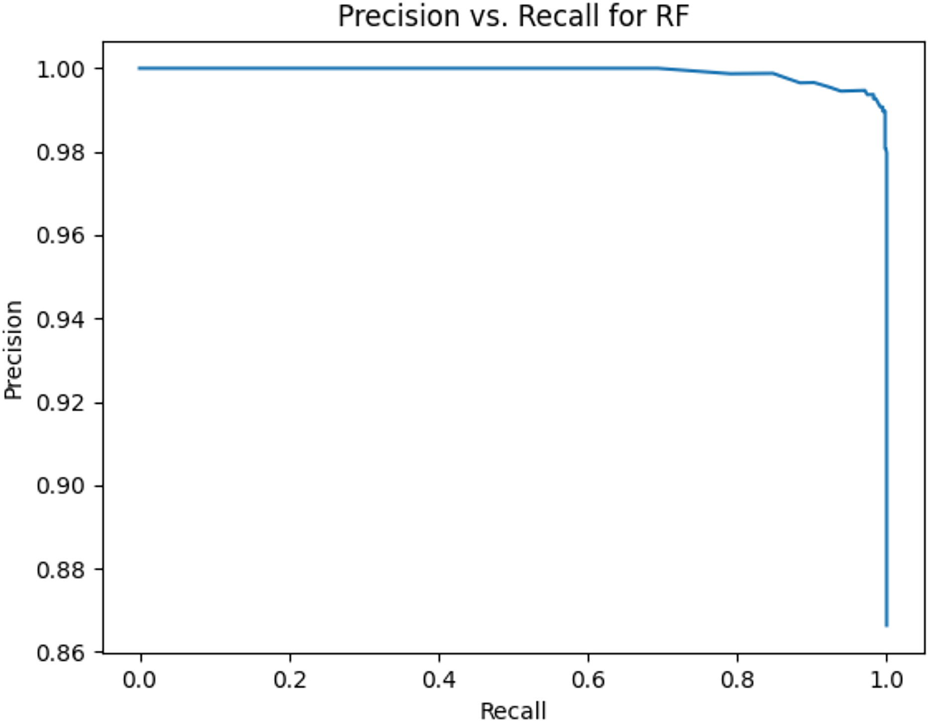
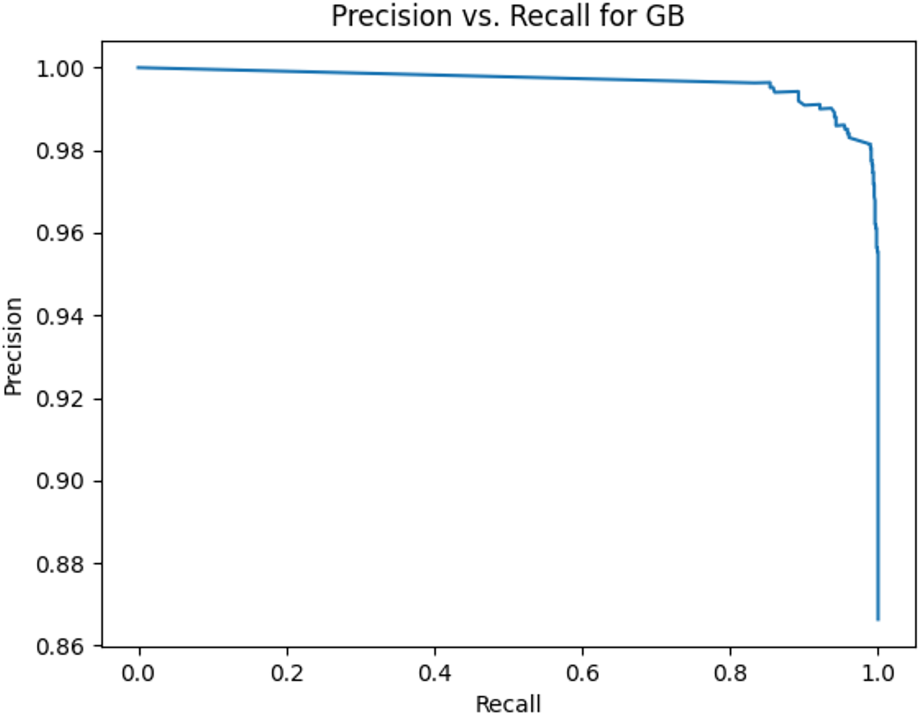
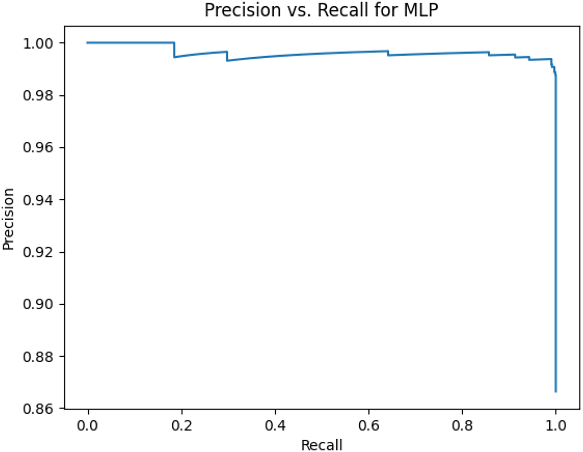
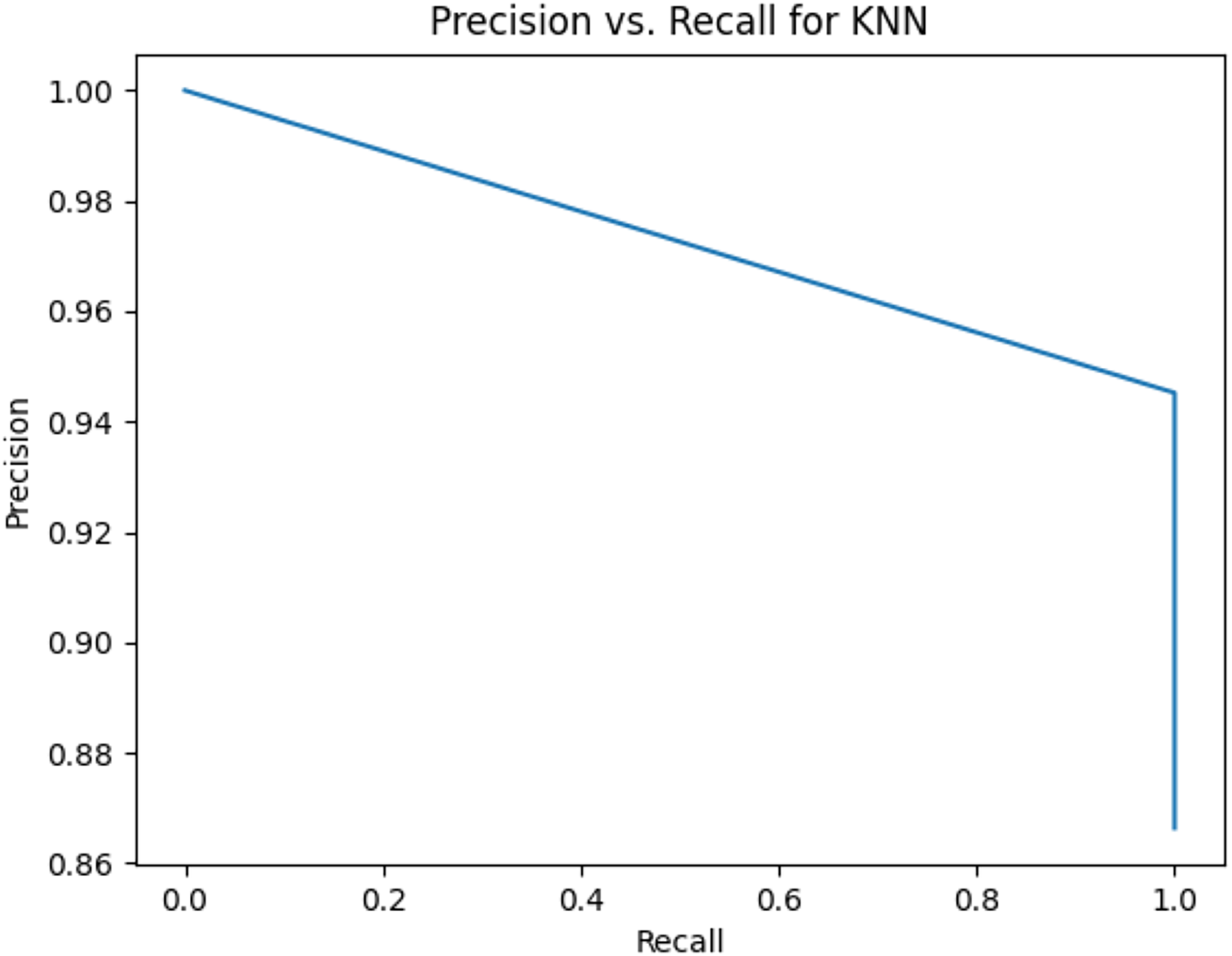
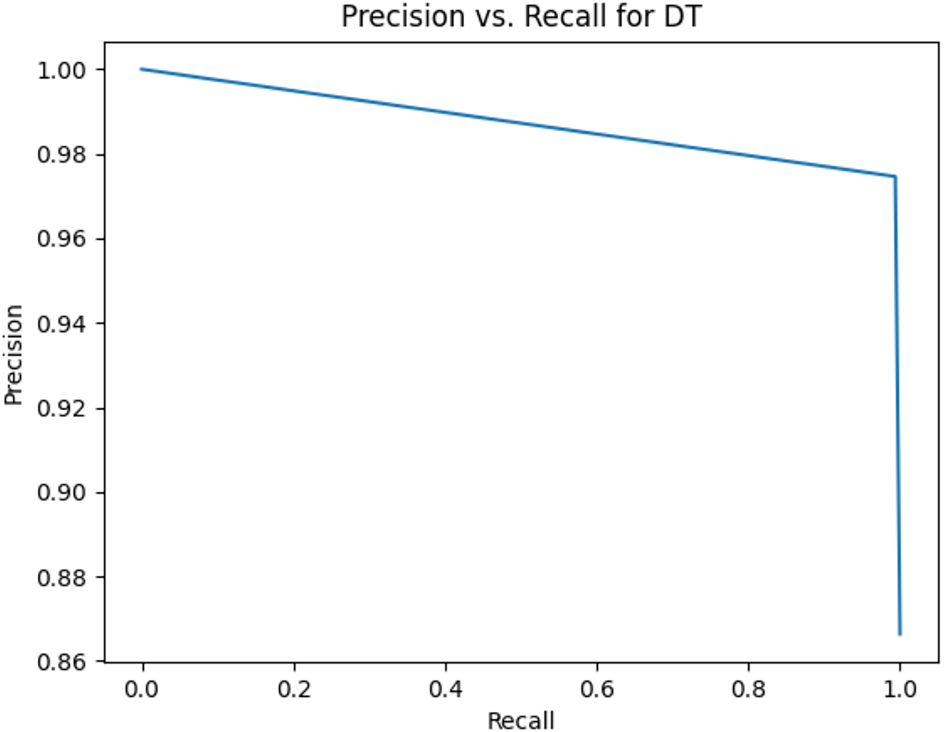
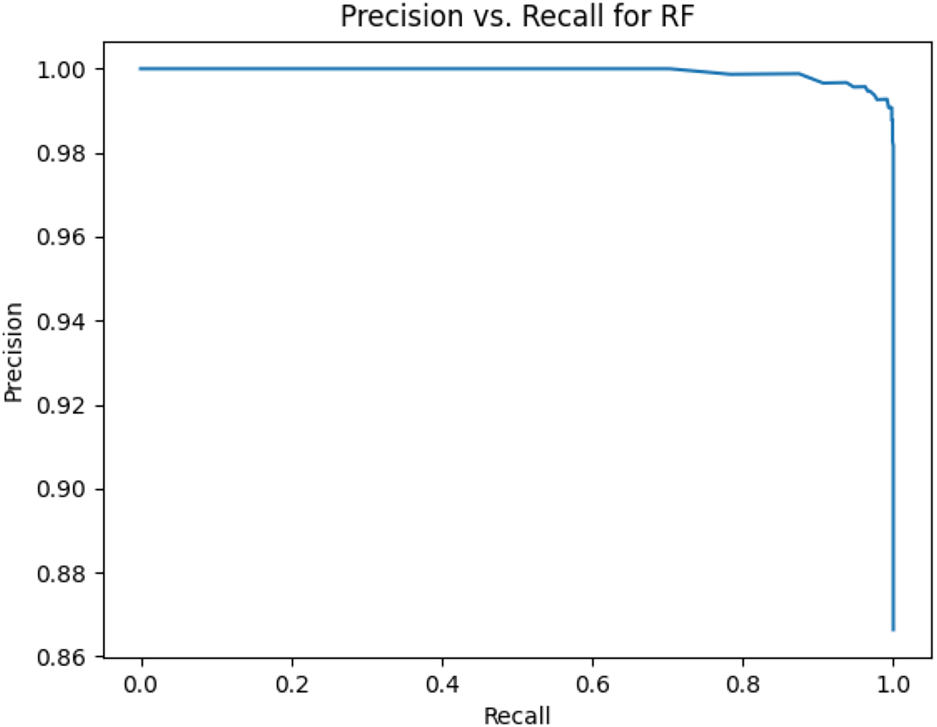
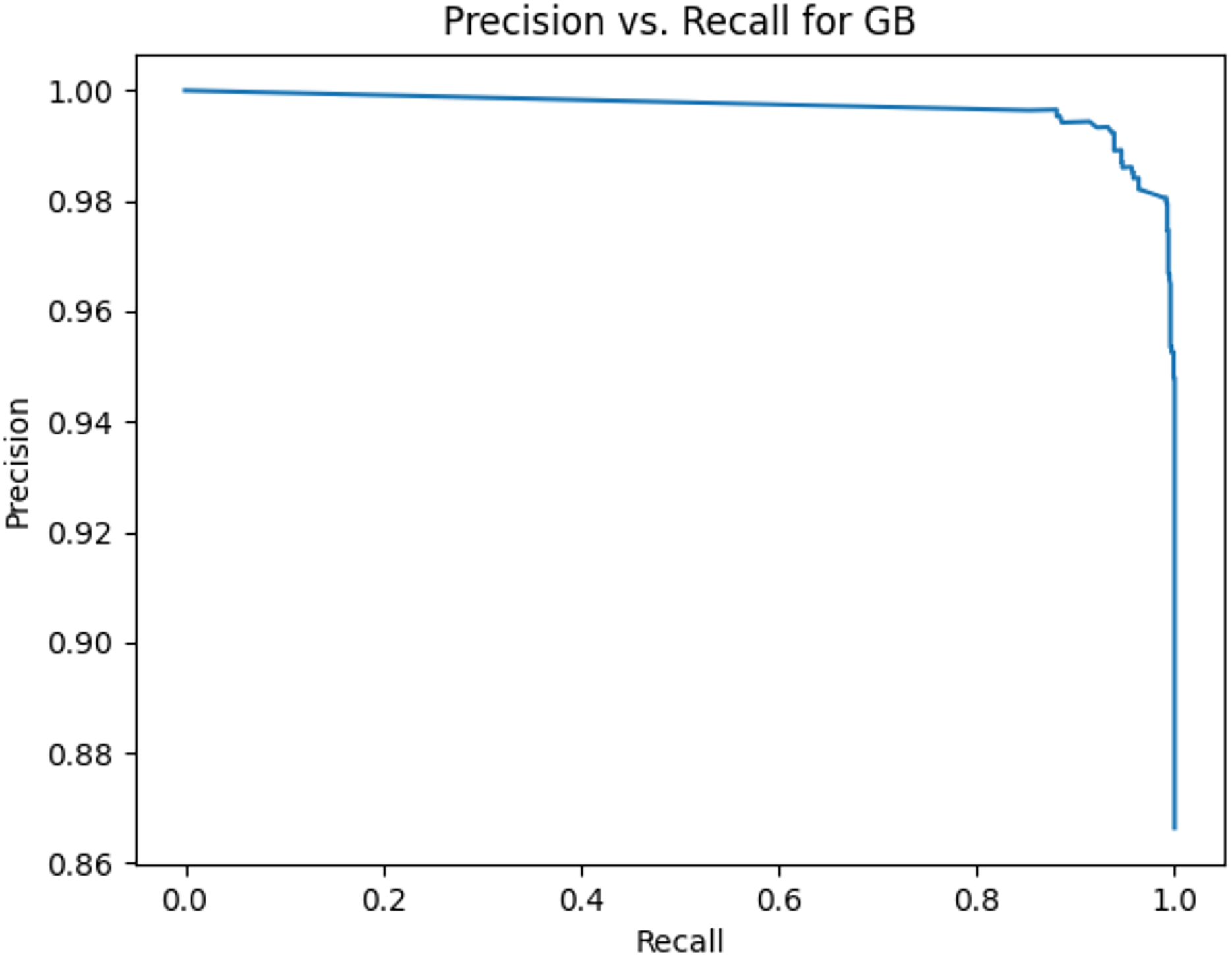
This sub-subsection presents the precision-recall curves and the areas under precision-recall curves for KNN, DT, RF, GB, MLP, and SVM algorithms. The imbalanced dataset is applied. A comparison is made among these algorithms based on the precision-recall curves and the area under precision-recall curves. Stemming and lemmatization are used. For stemming, the precision-recall curves for KNN, DT, RF, GB, MLP, and SVM are shown in Figs. 2, 3, 4, 5, 6, and 7, respectively. Precision-recall curves for KNN, DT, RF, GB, MLP, and SVM using lemmatization are shown in Figs. 8, 9, 10, 11, 12, and 13, respectively. Table 11 shows the area under precision-recall curves for the compared algorithms.

Figure 2: Precision vs. recall for KNN using stemming and the imbalanced dataset.
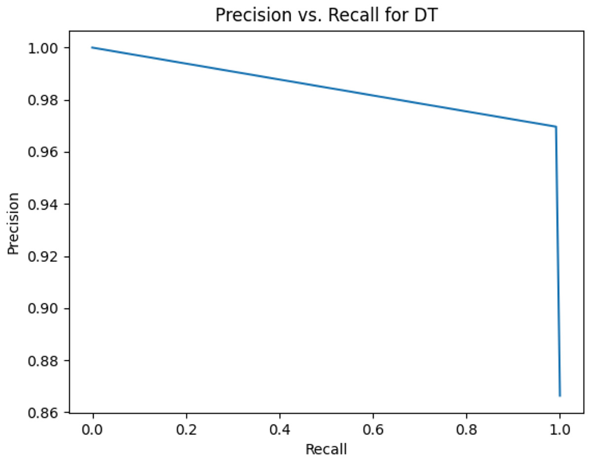
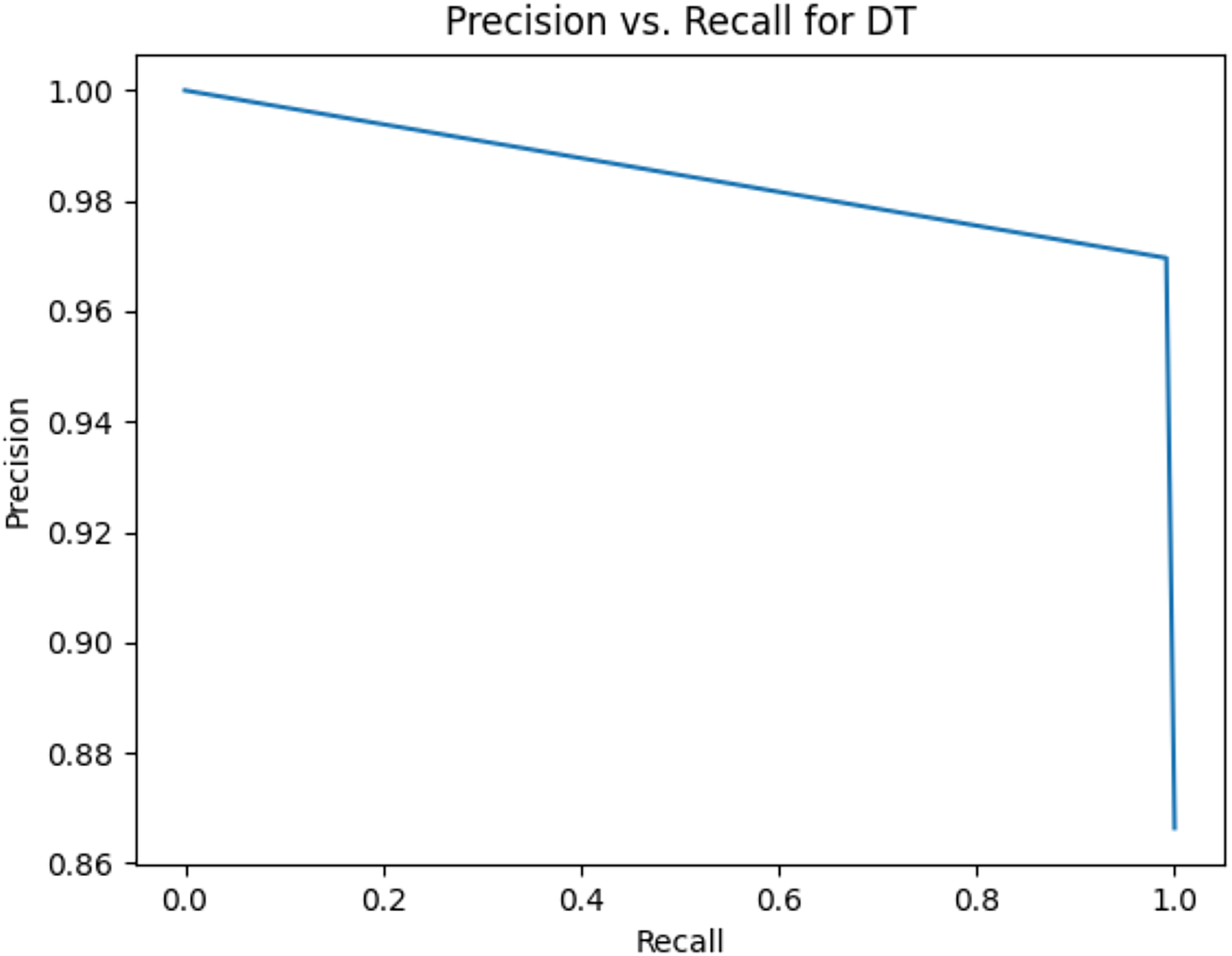
Figure 3: Precision vs. recall for DT using stemming and the imbalanced dataset.

Figure 4: Precision vs. recall for RF using stemming and the imbalanced dataset.
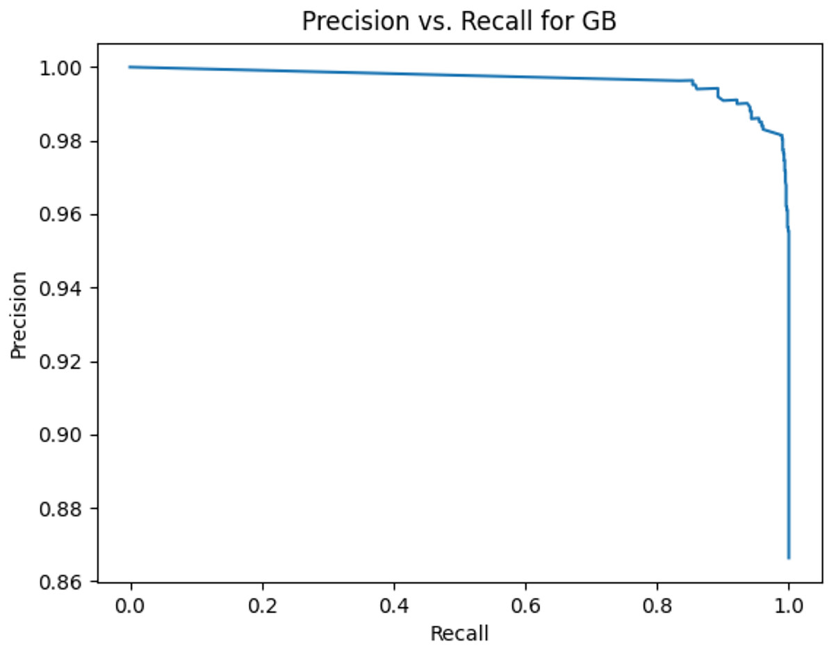
Figure 5: Precision vs. recall for GB using stemming and the imbalanced dataset.

Figure 6: Precision vs. recall for MLP using stemming and the imbalanced dataset.

Figure 7: Precision vs. recall for SVM using stemming and the imbalanced dataset.
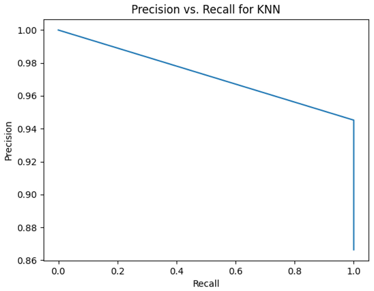
Figure 8: Precision vs. recall for KNN using lemmatization and the imbalanced dataset.
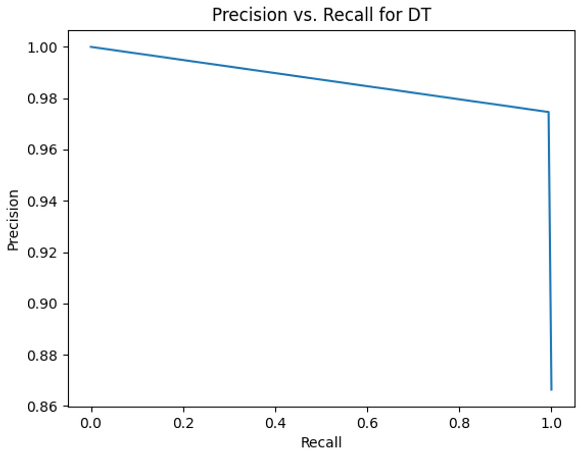
Figure 9: Precision vs. recall for DT using lemmatization and the imbalanced dataset.
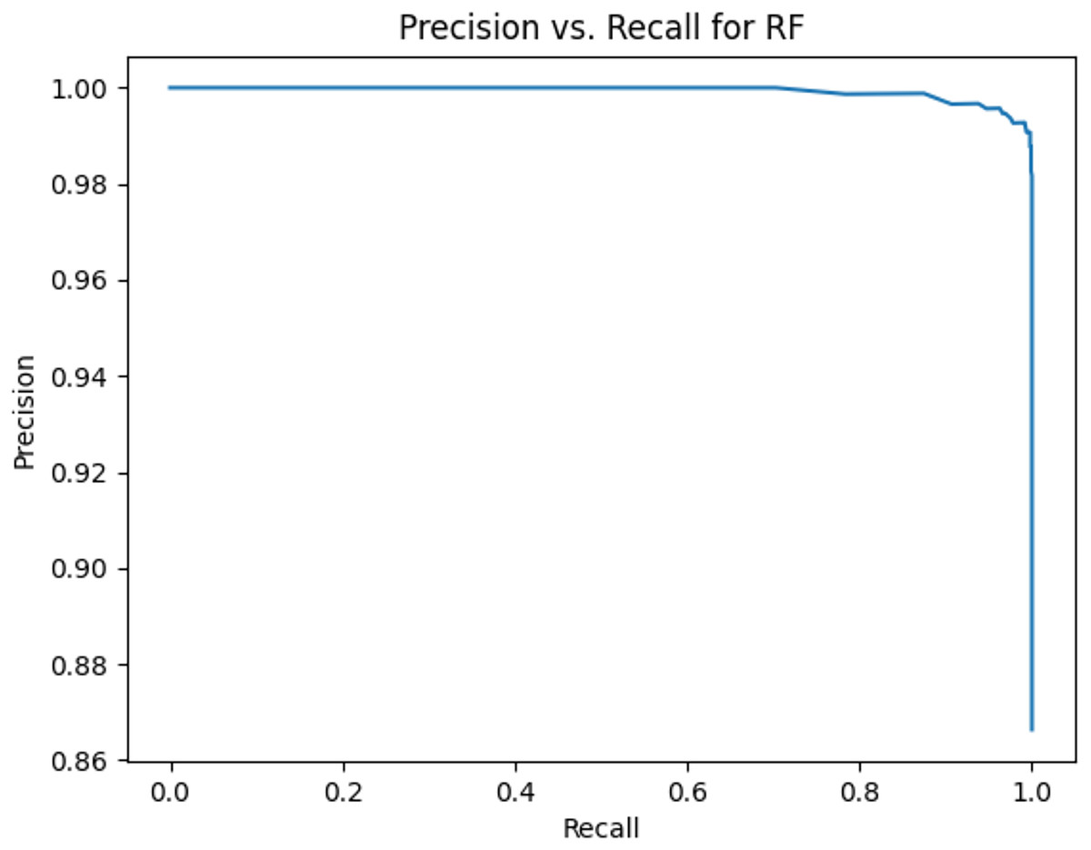
Figure 10: Precision vs. recall for RF using lemmatization and the imbalanced dataset.
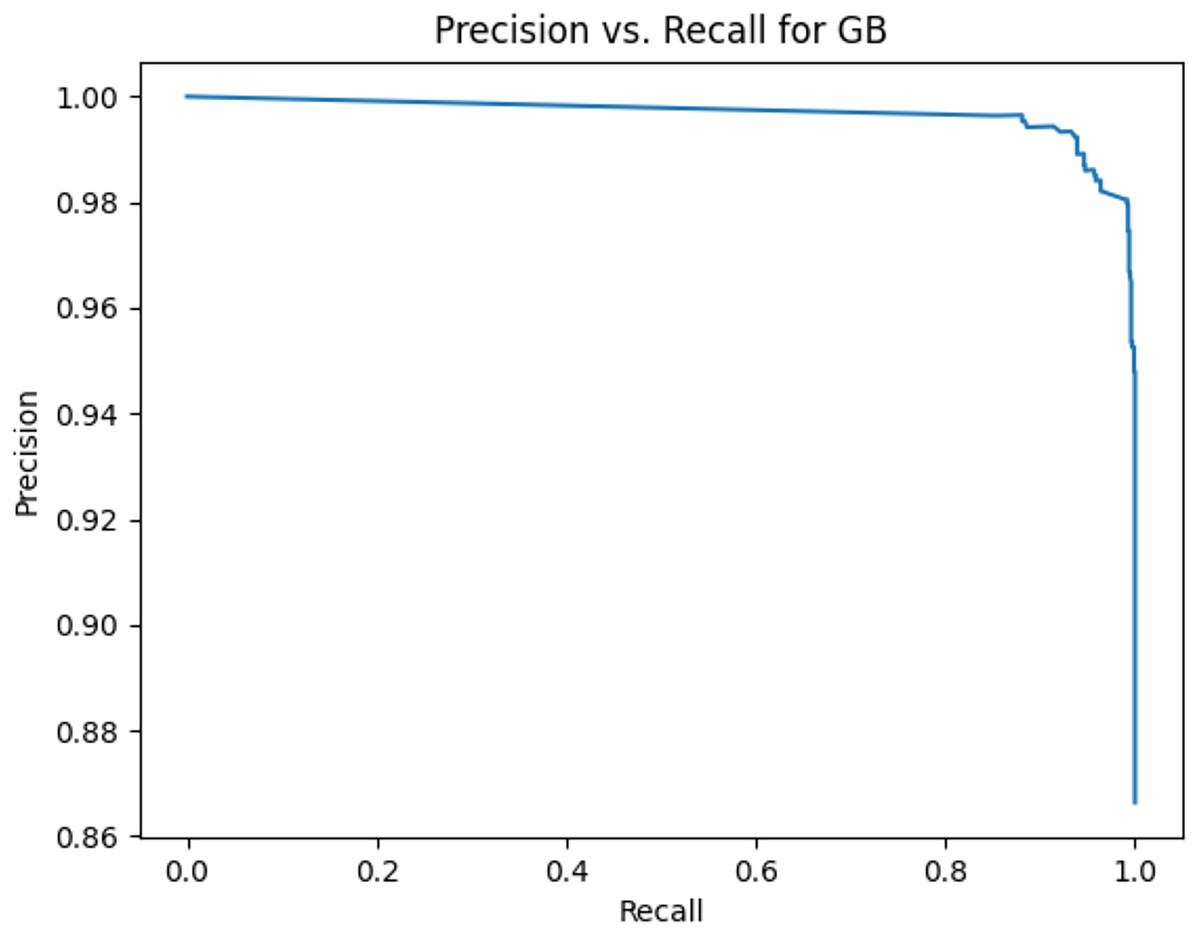
Figure 11: Precision vs. recall for GB using lemmatization and the imbalanced dataset.
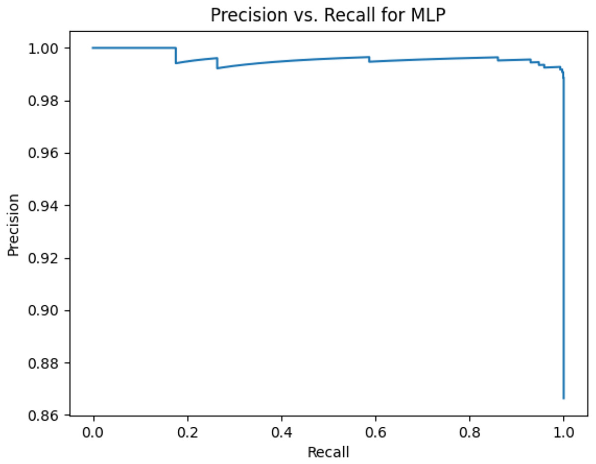
Figure 12: Precision vs. recall for MLP using lemmatization and the imbalanced dataset.
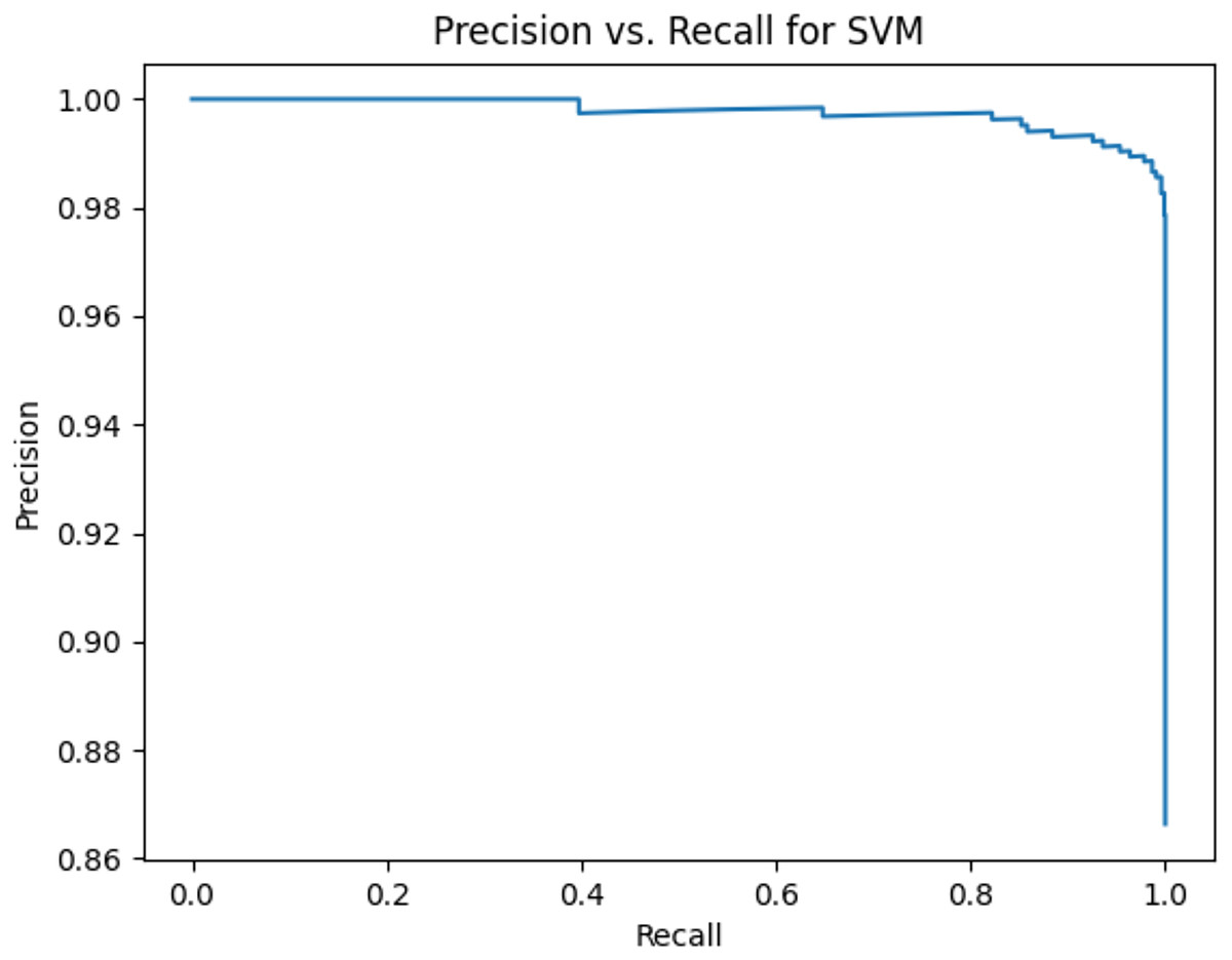
Figure 13: Precision vs. recall for SVM using lemmatization and the imbalanced dataset.
| Algorithm | The area under precision-recall curve based on stemming | The area under precision-recall curve based on lemmatization |
|---|---|---|
| KNN | 0.973065622 | 0.97260274 |
| Decision Tree | 0.984264471 | 0.986894638 |
| Random Forest | 0.999135405 | 0.999278528 |
| Gradient Boosting | 0.996588804 | 0.99682781 |
| Multi-Layer Perceptron | 0.996211744 | 0.995947991 |
| SVM | 0.997582607 | 0.997641867 |
Figures 2–13 illustrate the precision vs. recall results based on different classification thresholds. Precision-recall curves are employed to evaluate the performance of classification models (Precision-Recall Curve, 2024). This sub-subsection uses precision-recall curves to evaluate the performance of the compared algorithms when an imbalanced dataset is used. Figures 2–13 show high areas under the precision-recall curves. Therefore, both precision and recall results are high, which leads to the classification algorithm models performing well.
Table 11 shows the area under precision-recall curves for the compared algorithms using stemming and lemmatization. This table reveals that the results of the areas under precision-recall curves for the compared algorithms using stemming and lemmatization are high. Therefore, the performance of these algorithms is acceptable. In this table, the highest results are for RF, which means the model performance of RF is the highest, and RF has the highest ability to balance between precision and recall. SVM has the second highest model performance because SVM has the second highest results for the area under the precision-recall curve. SVM has the second highest ability to offer balancing between precision and recall. GB has the third highest model performance because GB has the third highest results for the area under the precision-recall curve. GB has the third highest ability to present balancing between precision and recall. MLP has the fourth highest model performance because MLP has the fourth highest results for the area under the precision-recall curve. MLP has the fourth highest ability to present balancing between precision and recall. The model performance of DT is better than the model performance of KNN because the results of the area under the precision-recall curve for DT are better than those of KNN. DT has a better ability to balance precision and recall than KNN.
Comparison between the proposed model and other models
This subsection presents a comparison between the proposed model and other models (Tekerek, 2017; Nyamathulla et al., 2022; Moutafis, Andreatos & Stefaneas, 2023), as well as the optimized algorithm from Fatima et al. (2023), based on various machine learning algorithms, to determine which provides the best classification results.
The accuracy results (in percentage) of the models and the optimized algorithm are shown in Table 12, while the precision/macro average precision and recall/macro average recall results for the proposed model, the model in Nyamathulla et al. (2022), and the optimized algorithm (Fatima et al., 2023) are presented in Tables 13 and 14, respectively. The F1-score/macro average F1-score results for the proposed model and the optimized algorithm are illustrated in Table 15.
| The proposed model | Model in Tekerek (2017) | Model in Nyamathulla et al. (2022) | csv by F. Qureshi in Moutafis, Andreatos & Stefaneas (2023) |
The optimized algorithm in Fatima et al. (2023) | ||
|---|---|---|---|---|---|---|
| Algorithm | Accuracy based on stemming | Accuracy based on lemmatization | Result (%) | Accuracy | Accuracy | Accuracy |
| KNN | 94.977578% | 94.88789% | 95.1381% | 92% | 95.51% | NA |
| Decision Tree | 97.2197% | 96.7713% | NA | 90% | 97.85% | NA |
| Random Forest | 97.578% | 97.7578% | 97.4345% | 91% | 98.11% | 97.49% |
| Gradient Boosting | 95.06726% | 95.15695% | NA | NA | 95.9% | NA |
| Multi-Layer Perceptron/Neural Network (NN)/Recurrent Neural Network (RNN) | 98.74439% (Multi-Layer Perceptron) | 98.6547% | NA | NA | 98.23% (NN) 98.3% (RNN) |
97.94% |
| SVM/LSVC | 98.29596% | 98.4753% | 98.3315% | 90% | 98.39% | 97.85% |
| The proposed model | Model in Nyamathulla et al. (2022) | The optimized algorithm in Fatima et al. (2023) | ||
|---|---|---|---|---|
| Algorithm | Precision based on stemming | Precision based on lemmatization | Precision | Macro average precision |
| KNN | 94.5205% | 94.428% | 65% | NA |
| Decision Tree | 97.558% | 98.2365% | 87% | NA |
| Random Forest | 97.280966767% | 97.477% | 87% | 98.44% |
| Multi-Layer Perceptron | 98.5714% | 98.4709% | NA | 97.85% |
| SVM/LSVC | 98.0710659898% | 98.2706% | 80% | 98.79% |
| The proposed model | Model in Nyamathulla et al. (2022) | The optimized algorithm in Fatima et al. (2023) | ||
|---|---|---|---|---|
| Algorithm | Recall based on stemming | Recall based on lemmatization | Recall | Macro average recall |
| KNN | 100% | 100% | 99% | NA |
| Decision Tree | 99.275% | 98.033% | 97% | NA |
| Random Forest | 100% | 100% | 98% | 92.07% |
| Multi-Layer Perceptron | 100% | 100% | NA | 93.18% |
| SVM/LSVC | 100% | 100% | 99% | 92.46% |
| The proposed model | The optimized algorithm in Fatima et al. (2023) | ||
|---|---|---|---|
| Algorithm | F1-score based on stemming | F1-score based on lemmatization | Macro average F1-score |
| Random Forest | 98.6217% | 98.7225% | 94.32% |
| Multi-Layer Perceptron | 99.2805755% | 99.22958% | 95.35% |
| SVM/LSVC | 99.0261% | 99.1277578% | 95.04% |
The term Result(%) represents the success rate (Tekerek, 2017). For each label, the precision, recall, and F1-score results are computed. The arithmetic mean of precision results is the macro average precision (Pedregosa et al., 2011), the arithmetic mean of recall results is the macro average recall (Pedregosa et al., 2011), and the arithmetic mean of F1-score results is the macro average F1-score (Pedregosa et al., 2011). These means are unweighted (Pedregosa et al., 2011).
The results for the model in Nyamathulla et al. (2022) were obtained using the CountVectorizer and SMOTE techniques.
In Fatima et al. (2023), the proposed optimized machine learning algorithm improves accuracy, macro average precision, macro average recall, and macro average F1-score through hyperparameter tuning. The best results are achieved using different parameter optimization approaches, including manual search, random search, grid search, and GA. Additionally, the comparison involves optimized algorithms based on linear support vector classifier (LSVC), RF, and MLP, which all employ CountVectorizer.
For the LSVC-based optimized algorithm in Fatima et al. (2023), the best results for accuracy, macro average precision, and macro average F1-score are achieved using GA, while the best macro average recall result is obtained with manual search.
For the RF-based optimized algorithm in Fatima et al. (2023), the best accuracy results are achieved using general search cross-validation (GSCV), random search cross-validation (RSCV), or GA. The best macro average precision is obtained with Manual Search, and the best results for macro average recall and macro average F1-score are achieved using GA.
For the MLP-based optimized algorithm in Fatima et al. (2023), the best results for accuracy, macro average precision, macro average recall, and macro average F1-score are obtained using GSCV.
The model with better accuracy results is able to detect the correct class labels more consistently than other models.
Table 12 shows that the proposed model based on SVM achieves better accuracy results using lemmatization compared to the models in Tekerek (2017), Nyamathulla et al. (2022), Moutafis, Andreatos & Stefaneas (2023) and the optimized algorithm in Fatima et al. (2023). It also indicates that the model in Moutafis, Andreatos & Stefaneas (2023) delivers the best accuracy results when using the KNN, DT, RF, and GB algorithms. Furthermore, the SVM-based model in Moutafis, Andreatos & Stefaneas (2023) outperforms the proposed model based on stemming, the model in Tekerek (2017), the model in Nyamathulla et al. (2022), and the optimized algorithm in Fatima et al. (2023). The SVM-based model in Tekerek (2017) also achieves better performance than the proposed model based on stemming, the model in Nyamathulla et al. (2022), and the optimized algorithm in Fatima et al. (2023). The accuracy results of the proposed model based on stemming and using SVM exceed those of the model in Nyamathulla et al. (2022) and the optimized algorithm. The accuracy of the optimized algorithm based on LSVC surpasses the SVM-based model in Nyamathulla et al. (2022). The KNN-based model in Tekerek (2017) performs better than both the proposed model and the model in Nyamathulla et al. (2022). Additionally, the proposed model based on KNN achieves better accuracy than the model in Nyamathulla et al. (2022). The proposed model based on RF provides better accuracy results than the performance in Tekerek (2017), as well as the results in Nyamathulla et al. (2022) and the optimized algorithm. The optimized algorithm based on RF also outperforms both the model in Tekerek (2017) and the model in Nyamathulla et al. (2022). Additionally, the RF-based model in Tekerek (2017) performs better than the model in Nyamathulla et al. (2022). The proposed model based on DT delivers better accuracy results than the model in Nyamathulla et al. (2022).
The proposed model based on MLP surpasses the accuracy of the model in Moutafis, Andreatos & Stefaneas (2023) (which uses NN and RNN algorithms) and the optimized algorithm. Moreover, the models based on NN and RNN in Moutafis, Andreatos & Stefaneas (2023) perform better than the optimized algorithm.
It is noted in Table 13 that the optimized algorithm based on RF and LSVC outperforms both the proposed model and the model in Nyamathulla et al. (2022) in terms of Macro Average Precision. This is because the optimized algorithm has a lower percentage of false positives compared to both the proposed model and the model in Nyamathulla et al. (2022). However, the proposed model based on the MLP algorithm achieves better precision than the macro average precision of the optimized algorithm, as the optimized algorithm has a higher percentage of false positives than the proposed model.
Table 13 also indicates that the proposed model based on KNN, DT, RF, and SVM algorithms yields better precision results than the model in Nyamathulla et al. (2022), due to the proposed model having a lower percentage of false positives.
As shown in Table 14, the proposed model based on RF and SVM provides better recall results than the RF and SVM models in Nyamathulla et al. (2022) and the macro average recall results for the optimized algorithm based on RF and LSVC. This is because the proposed model has fewer incorrectly predicted actual positive classes compared to the model in Nyamathulla et al. (2022) or the optimized algorithm. Moreover, the RF and SVM models in Nyamathulla et al. (2022) have better recall results than the macro average recall results of the optimized algorithm based on RF and LSVC.
The proposed model based on MLP also delivers better recall results than the Macro Average Recall of the optimized algorithm, as it incorrectly predicts fewer actual positive classes than the optimized algorithm.
Table 14 shows that the proposed model based on KNN and DT algorithms exhibits better recall results than the corresponding recall results of the model based on these algorithms in Nyamathulla et al. (2022).
The recall results for the proposed model based on KNN, RF, MLP, and SVM are all 100%.
Table 15 presents the F1-score for the proposed model and the macro average F1-score for the optimized algorithm based on RF, MLP, and SVM/LSVC. It is evident from Table 15 that the proposed model achieves better F1-score results for these algorithms than the macro average F1-score of the optimized algorithm. This is because the proposed model has fewer incorrect predictions for both actual positive and negative classes compared to the optimized algorithm.
Implications
This subsection is divided into two parts: ‘Theoretical Implications’ presents the theoretical implications, and ‘Practical Implications’ discusses the practical implications.
Theoretical Implications
This subsection presents the classification results that have a significant impact on this research area. The results from the proposed model, which is based on NLP and machine learning algorithms, are promising, as they demonstrate high performance.
The accuracy results are notably high, particularly due to the use of the MLP, which outperforms both the previous model (Moutafis, Andreatos & Stefaneas, 2023) and the optimized algorithm (Fatima et al., 2023). Additionally, the accuracy of the SVM using lemmatization is also improved, surpassing the accuracy results of earlier models (Tekerek, 2017; Nyamathulla et al., 2022; Moutafis, Andreatos & Stefaneas, 2023) and the optimized algorithm.
The precision results of the proposed model based on MLP are also enhanced, exceeding the macro average precision of the optimized algorithm. Furthermore, the precision results of the proposed model based on KNN, DT, RF, and SVM are improved compared to those of the previous model (Nyamathulla et al., 2022).
The recall and F1-score results for RF, MLP, and SVM models are also better than the macro average recall and macro average F1-score results for the optimized algorithm. Moreover, the recall results for KNN, DT, RF, and SVM models show improvement compared to the recall results of the previous model (Nyamathulla et al., 2022).
The most notable outcome is that the KNN, RF, MLP, and SVM models exhibit no false negative cases, leading to recall results of 1.
Practical Implications
Based on the results of the proposed model, which incorporates NLP and machine learning algorithms, the model can be applied to the following real-world scenarios:
The proposed model can be used as a spam filter system to detect SMS messages containing phishing attempts or malware links. This would help protect users’ data, finances, and devices.
By identifying spam SMS messages, the proposed model can reduce the volume of messages received, thereby conserving device resources and saving users’ time.
The proposed model ensures that legitimate (ham) SMS messages are delivered to users without interference.
Limitations
The proposed model, based on NLP and machine learning algorithms, has the following limitations:
Some legitimate (ham) SMS messages are misclassified as spam by the machine learning models. This results in recipients missing important messages, which could contain critical information.
The DT and GB models misclassified some spam SMS messages as legitimate. This allows spam SMS messages to reach recipients, potentially containing phishing or malware links. This poses a risk to recipients by exposing them to data theft, financial loss, or malware that could compromise their devices and data.
Future work
The future directions for this research study are as follows:
Applying the proposed machine learning model to datasets of varying sizes.
Evaluating the performance of the machine learning models using TF-IDF vectorizer as the feature extraction method.
Developing models based on other machine learning and deep learning algorithms (LeCun, Bengio & Hinton, 2015) to further enhance the classification performance.
Conclusions
SMS is widely used for communication between individuals. However, spam SMSs are unwanted as they can contain malicious links, advertisements, or phishing attempts. The problem of spam SMSs can be addressed through a filter system capable of detecting and blocking spam while allowing only legitimate (ham) SMSs to be delivered.
This article proposed a data-driven model using NLP and machine learning algorithms to detect both spam and ham SMSs. The machine learning algorithms used in the proposed model include KNN, DT, RF, GB, MLP, and SVM.
There are no overfitting and also no dataset bias. In addition, the accuracy results are high, and this leads to small number of misclassification cases.
These models were compared based on classification metrics such as accuracy, precision, recall, and F1-score to determine which algorithm offers the best performance. This comparison helps identify the most effective machine learning model for detecting spam and ham SMSs.
Additionally, the proposed model was evaluated against related works (Tekerek, 2017; Nyamathulla et al., 2022; Moutafis, Andreatos & Stefaneas, 2023; Fatima et al., 2023) to assess its performance in comparison to previous approaches.
The key findings are as follows:
For stemming and lemmatization, MLP achieved the best accuracy, precision, and F1-score using the balanced or imbalanced datasets. KNN, RF, MLP, and SVM all produced the same and the best recall results.
The precision-recall curves were used to evaluate the performance of the classification models of the compared algorithms using the imbalanced dataset for stemming and lemmatization. The results showed that the performance of the classification models of the compared algorithms is acceptable.
The results of the areas under the precision-recall curves are high for the compared algorithms using the imbalanced dataset, stemming, and lemmatization, which provides acceptable performance for the compared algorithms.
RF generated the highest results for areas under the precision-recall curves, indicating that RF’s model performance is the highest and most able to balance precision and recall.
The results showed satisfactory classification results, where all the classification results are greater than 0.9.
The MLP model outperformed the model in Moutafis, Andreatos & Stefaneas (2023) in terms of accuracy. The accuracy of the SVM model using lemmatization surpassed the accuracy results of the model in Tekerek (2017), as well as the models in Nyamathulla et al. (2022), Moutafis, Andreatos & Stefaneas (2023), and the optimized algorithm (Fatima et al., 2023). KNN, DT, and RF models delivered better precision results than the model in Nyamathulla et al. (2022). The MLP model outperformed the macro average precision results of the optimized algorithm. The proposed model based on KNN, DT, RF, and SVM outperformed the model in Nyamathulla et al. (2022) in terms of recall. RF, MLP, and SVM models achieved higher recall results than the macro average recall results of the optimized algorithm. The MLP model produced better F1-score results than the macro average F1-score results for the optimized algorithm.
The practical advantages of the proposed model are significant. The model can function as a detection system for spam and ham SMSs, improving SMS security by ensuring only ham SMSs reach users while blocking spam. This approach protects users’ data and devices by preventing malicious or unsolicited messages from being delivered. Furthermore, the model can reduce the time spent handling spam SMSs, allowing users to focus on important messages. By blocking spam and allowing only ham SMSs, the model helps conserve device resources. It also allocates more space for storing ham SMSs, ensuring important messages are not lost.
The research questions of this article have been answered as follows: The proposed model based on NLP and machine learning algorithms can detect spam and ham SMS messages with high accuracy. This leads to secure users’ information and preserves mobile device resources by allocating more resources for ham SMS messages. In addition, the results showed which machine learning model is more effective in detecting spam SMS messages and which machine learning algorithm offers the most satisfactory classification results among the compared models.
The users’ information can be secured by detecting spam SMS messages that contain malicious links, such as those that have malware and phishing websites. If a user receives a spam SMS message containing a malicious link with malware and clicks it, the malware is downloaded to the user’s device, potentially compromising the user’s security. Suppose the malicious link leads to a phishing website. When the user opens it, the malicious link directs the user to the phishing website, allowing cybercriminals to deceive the user by stealing their information and financial assets.
The proposed model, based on NLP and machine learning algorithms, helps detect spam SMS messages and thereby secure the user’s information.
Based on the achieved results of the proposed model, which is based on NLP and machine learning algorithms, the proposed model can serve as a filter system to detect spam and ham SMS messages. The satisfactory results of the proposed model indicate that it can effectively block spam SMSs, which have a significant impact on the user’s security and privacy. Additionally, the proposed model protects users’ assets and information by blocking spam SMSs. The proposed model blocks spam SMSs that carry advertisements, malicious links, and phishing websites, thereby protecting both the privacy and security of users.
The results are valid because of the following reasons: the classification results were measured based on the balanced dataset to solve the unequal data distribution between classes. The classification results, precision-recall curve, and the area under the precision-recall curve were measured based on the imbalanced dataset to consider the real-world distribution of data between classes. The proposed model was compared with other existing models.
Supplemental Information
SMS spam.
The dataset contains two columns: the first column represents the labels, and the second contains the SMS messages.
Computer Code.
Stemming is working in the upload file. To make Lemmatization working. Remove # symbol before the following lines of code:
#lemmatizer = WordNetLemmatizer()
#lemmatizer_tokens = [lemmatizer.lemmatize(token) for token in tokens if token not in stop_words]
#lemmatizer_tokens = ’ ’.join(lemmatizer_tokens)
#Messages.append(lemmatizer_tokens)
In addition, make the following lines of code for Stemming as comments by adding # symbol at the beginning of each of these lines of code:
stm = PorterStemmer()
stemming_tokens = [stm.stem(token) for token in tokens if token not in stop_words]
stemming_tokens = ’ ’ .join(stemming_tokens) Messages.append(stemming_tokens)
Note: The lines of code that started by # symbol are comments
Computer Code-Using the Imbalanced Dataset.
Stemming is working in the upload file. To make Lemmatization working. Remove # symbol before the following lines of code: #lemmatizer = WordNetLemmatizer() #lemmatizer_tokens = [lemmatizer.lemmatize(token) for token in tokens if token not in stop_words] #lemmatizer_tokens = ’ ’.join(lemmatizer_tokens) #Messages.append(lemmatizer_tokens) In addition, make the following lines of code for Stemming as comments by adding # symbol at the beginning of each of these lines of code stm = PorterStemmer() stemming_tokens = [stm.stem(token) for token in tokens if token not in stop_words] stemming_tokens = ’ ’ .join(stemming_tokens) Messages.append(stemming_tokens) Note: The lines of code that started by # symbol are comments