
Predicting software developer sentiment on self-admitted technical debt
- Published
- Accepted
- Received
- Academic Editor
- Marieke Huisman
- Subject Areas
- Artificial Intelligence, Software Engineering
- Keywords
- Technical debt, Self-admitted technical debt, Sentiment prediction, Generative pre-trained models, GPT
- Copyright
- © 2025 Zhang et al.
- Licence
- This is an open access article distributed under the terms of the Creative Commons Attribution License, which permits unrestricted use, distribution, reproduction and adaptation in any medium and for any purpose provided that it is properly attributed. For attribution, the original author(s), title, publication source (PeerJ Computer Science) and either DOI or URL of the article must be cited.
- Cite this article
- 2025. Predicting software developer sentiment on self-admitted technical debt. PeerJ Computer Science 11:e3227 https://doi.org/10.7717/peerj-cs.3227
Abstract
Technical debt is a metaphor for sacrificing long-term code quality in order to achieve short-term project goals. The technical debt that developers intentionally introduce into project is called self-admitted technical debt (SATD), which usually exists in the form of code comments in software projects. The existence of SATD poses a huge challenge to software quality and robustness. Analyzing the sentiments of SATD helps to understand the behavioral habits of developers when annotating SATD. In order to explore the performance of generative pre-trained models in SATD sentiment prediction, a SATD sentiment prediction method based on the GPT-3.5-turbo fine-tuning model is proposed, and research is carried out on 18 open source projects. Empirical results show that, compared with a set of traditional machine learning and deep learning techniques, the fine-tuning GPT-3.5-turbo model improves the evaluation indicators precision, recall and F1-score by 14.2%, 11.5%, and 17.3%, respectively. The effectiveness of the SATD sentiment prediction method based on GPT-3.5-turbo is verified, indicating the potential of generative pre-trained models to capture nuanced complex sentiment—i.e., developer comments that combine neutral technical observations with subtle negative cues such as hesitation or frustration. However, our comparison does not include recent large language model (LLM)-based approaches, which are reserved for future investigation.
Introduction
Technical debt (TD) (Cunningham, 1992) refers to compromises made in system design, code quality, etc. during software development in order to quickly deliver features or meet short-term requirements, which may lead to long-term disadvantages (Izurieta et al., 2017; Kruchten, Nord & Ozkaya, 2012; Li, Avgeriou & Liang, 2015; Lim, Taksande & Seaman, 2012; Nord et al., 2016; Pointa & Dagstuhl, 2015). They increase the maintenance burden, reduce code quality, and may make future changes more time-consuming and expensive, which requires interest repayment. This concept compares the consequences of technical decisions to financial debt, emphasizing the trade-off between short-term benefits and long-term risks. Self-admitted technical debt (SATD) is a special form of technical debt, which refers to technical debt explicitly acknowledged by developers in software artifacts such as code comments, documents, and commit messages (Potdar & Shihab, 2014). By recording these technical compromises, development teams can better understand and track the causes and impacts of technical debt. However, the accumulation of SATD may have a negative impact on software quality, increase subsequent maintenance costs, and even lead to maintenance crises (Xiao et al., 2024).
Since the concept of SATD was proposed, academia and industry have conducted extensive research on its identification and management. Early research mainly identified SATD through static source code analysis, using keywords (such as TODO, FIXME) in code comments as identifiers of technical debt (Maldonado & Shihab, 2015). These methods have made significant progress in SATD identification at the code level and can efficiently discover design debts or code defects that are explicitly acknowledged by developers. However, these methods have certain limitations in identifying other types of technical debt (such as documentation debt, requirements debt, etc.), especially technical debt that is not explicitly annotated or exists implicitly and is difficult to capture. In recent years, researchers have begun to explore the use of machine learning and deep learning technologies to improve the accuracy and coverage of SATD recognition. For example, Huang et al. (2018) proposed an automated method that combines multiple classifiers (traditional machine learning classifiers, such as Naive Bayes, support vector machine (SVM), etc.,) to detect SATD. These classifiers are trained on annotated data from open source projects to predict the presence of SATD in target projects. Studies show that these methods achieve good F1-scores in SATD detection. There are also studies using deep learning models such as convolutional neural networks (CNN) and long short-term memory networks (LSTM) to capture more complex semantic features (Li et al., 2024).
More importantly, Li et al. (2024) conducted one of the first systematic studies to apply large language model (LLM) to SATD detection. They extensively evaluated ChatGPT on zero-shot, few-shot BM25, and few-shot Chain of Thought (CoT) prompting strategies and found that LLM significantly outperformed traditional CNN, LSTM, and Transformer models, especially in terms of recall and interpretability. In addition, they proposed a fusion method (FSATD) that combines the predictions of ChatGPT with those of a small model to further improve the classification performance. Their work strongly demonstrated that LLM-based methods are very promising for the SATD detection task. However, their study mainly focused on SATD classification (i.e., whether a comment indicates technical debt) rather than the sentiment dimension of SATD, which remains underexplored.
Although research on the classification and detection of SATD is relatively mature, there is little in-depth discussion on the analysis of emotional expression in SATD. Currently, research on SATD sentiment analysis is still in its infancy. Fucci et al. (2021) systematically analyzed emotional expressions in SATD annotations for the first time in 2021. By analyzing 1,038 SATD comments from 10 open source projects, the proportion of SATD with negative sentiment is only 30%. Therefore, developers usually adopt a more neutral or objective expression when recording technical debt. In addition, the presence of negative sentiment is particularly evident in two specific SATD categories: functional issues (i.e., reviews that describe software functional defects or failures) and waiting issues (e.g., reviews involving tasks that are blocked by external dependencies such as third-party libraries or unresolved issues). In these categories, the proportion of negative sentiment in SATD reviews is as high as 49% and 46%, respectively. This suggests that developers may be more inclined to express frustration or dissatisfaction when technical debt involves functional defects or dependencies on external conditions.
However, existing sentiment analysis tools for SATD, such as Senti4SD (Calefato et al., 2018), face limitations when applied to this context. Fucci et al. (2021) evaluated the performance of several sentiment analysis tools in SATD detection and found that some negative comments were misclassified as neutral due to the presence of technology-specific terms. For example, the sentence “FIXME: This is a big pitfall because the parser expects scope names to be preserved as strings” was marked as negative by human judges but misclassified as neutral by Senti4SD. Fucci et al. (2021) concluded that sentiment analysis tools in software engineering may not fully capture the true emotional expressions of developers in SATD, especially when technical vocabulary is involved.
In the field of sentiment analysis, the Generative Pretrained Transformer (GPT) model has deeply learned the statistical laws and contextual associations of language through pre-training on massive text data, and can generate fluent and grammatical text (Kheiri & Karimi, 2023). Recent studies have shown that designing well-structured prompts for GPT models can significantly improve the performance of sentiment analysis tasks (Kheiri & Karimi, 2023). Therefore, this article proposes a SATD sentiment prediction method based on the generative pre-training model ChatGPT. By fine-tuning the ChatGPT model to adapt it to the SATD sentiment prediction task, we aim to improve the accuracy of sentiment analysis. Specifically, in order to fully mine the complex emotional expressions in SATD text, the pre-trained large language model ChatGPT was fine-tuned to build a SATD sentiment prediction model. Secondly, the performance of the fine-tuned GPT model in SATD sentiment prediction is systematically evaluated. By comparing it with machine learning methods and deep learning models, the effectiveness of the fine-tuned ChatGPT model in the SATD sentiment prediction task was verified, revealing the application potential of generative models in the field of sentiment analysis.
The main contributions of this article can be summarized as follows:
-
(1)
A generative model framework for SATD sentiment prediction is proposed. By fine-tuning the GPT model, its performance in complex sentiment capture tasks is systematically evaluated.
-
(2)
The performance of the fine-tuned GPT model is compared with traditional machine learning methods and deep learning models through experiments, and its potential advantages in SATD emotion recognition are demonstrated. The rest of this article introduces related work in SATD, presents the proposed method, describes the experimental setup and materials, analyzes the results, and summarizes the main findings and future directions.
Related work
Research on SATD
Regarding the study of SATD, Potdar & Shihab (2014) first analyzed the code comments in open source projects and found that developers tend to use specific keywords (such as “TODO” and “FIXME”) to mark the existence of technical debt. Subsequently, Maldonado & Shihab (2015) developed a pattern matching method to automatically detect SATD and divide it into categories such as defect debt, design debt, document debt, implementation debt, and test debt. Mainstream research focuses on the identification and classification of SATD. For example, Bavota & Russo (2016) redefined the SATD taxonomy and proposed more refined subcategories; in addition, Maipradit et al. (2020) introduced the concept of “on-hold” SATD to describe the comments left by developers while waiting for internal or external conditions of the project to be met. They further constructed a classifier specifically for detecting this type of “on-hold” SATD and achieved an average area under the curve (AUC) of 0.97 in the experiment (Maipradit et al., 2020). These studies have effectively improved the identification and classification methods of SATD, but there are still deficiencies in the systematic analysis of emotional factors, especially how sentiments affect the priority of technical debt management, which has not been deeply explored.
Sentiment analysis in software development
In recent years, sentiment analysis has gradually become popular and developed steadily in empirical software engineering research. Murgia et al. (2014) preliminarily explored the sentiments in software artifacts by manually annotating the problem reports of the Apache Foundation and found that developers expressed a variety of sentiments such as gratitude, joy, and sadness in the reports. Ortu et al. (2015) studied the correlation between sentiments in problems and repair time, and the results showed that negative sentiments (such as sadness) were associated with longer repair times. Mäntylä et al. (2016) analyzed the relationship between sentiments and bug priorities. By mining the sentiments in problem tracking comments, calculating valence (emotional polarity), arousal (emotional intensity), and dominance, it was found that bug reports are usually accompanied by more negative valence, and the higher the priority, the stronger the emotional arousal.
Fucci et al. (2021) focused on how developers communicate the presence of technical debt by manually labeling sentiment in SATD reviews. The results further confirmed the effectiveness of sentiment as a proxy for issues and priorities in the software development process. In addition, researchers in the field of requirements engineering also use sentiment analysis to support software maintenance and requirements classification. Panichella et al. (2015) classified the sentiment of user reviews on Google Play and Apple Store, while Maalej et al. (2016) combined sentiment and other text features to automatically classify application reviews into four categories: bug reports, feature requests, user experience, and text ratings.
In the study of negative sentiments in the software development process, Gachechiladze et al. (2017) studied anger and its direction in collaborative development, and trained an anger detection classifier by manually annotating sentences in Apache issue reports. Fucci et al. (2021) also focused on negative sentiments and verified its effectiveness in the problem of agent software development.
SATD detection and GPT-based sentiment classification
In recent years, large pre-trained language models (LLMs) have shown great potential in software engineering text analysis tasks. Li et al. (2024) evaluated ChatGPT’s ability to detect software technical debt (SATD) in a zero-shot setting. The results showed that ChatGPT outperformed traditional CNN, LSTM, and Transformer models in both precision and recall, especially in small sample or unsupervised scenarios. Kheiri & Karimi (2023) proposed SentimentGPT, a method for advanced sentiment analysis using GPT. They found that the performance of GPT models in sentiment classification tasks can be significantly improved by carefully designed prompt templates. For example, an effective prompt template can guide the model to focus on the emotional tendency and complex language features (such as irony, emoticons, etc.,) in tweets, rather than just the literal meaning. They tested SentimentGPT on the SemEval 2017 dataset and showed that its F1-score was more than 22% higher than that of advanced models such as Bidirectional Long Short-Term Memory (BiLSTM) with attention, Convolutional Neural Network–Gated Recurrent Neural Network (CNN-GRNN) hybrid model, and Robustly Optimized BERT Pretraining Approach (RoBERTa).
Materials and Methods
This study conducts sentiment analysis on technical debt comments marked by developers in the source code, aiming to deeply understand their emotional responses when facing technical debt. To ensure long-term accessibility and reproducibility, we have permanently archived the processed datasets and source code on Zenodo (Version v1, DOI: 10.5281/zenodo.15605579). Additionally, the README file with implementation details is available at https://github.com/yangxingguang/satd_sentiment_GPT/blob/main/README.md.
The datasets used in our experiments are provided by Fucci et al. (2021), extracted from open-source projects. These datasets have been uploaded and made publicly available by the authors. The datasets can be downloaded from the following URL:
3rd Party SATD Dataset URL: https://figshare.com/s/0b83bc75dbc9ea99f2f6?file=26027183 and https://figshare.com/s/0b83bc75dbc9ea99f2f6?file=26027201
First, the original dataset is processed to ensure that the model can adapt to the complex characteristics of the SATD corpus. The original dataset contains SATD annotations annotated by developers and their corresponding sentiment labels. These categories cover common situations in sentiment analysis, including Non-Negative, Negative, Neutral, Mixed, and No Agression. Specifically, “No Aggression” refers to the situation where the annotation does not express aggressive or offensive emotional content, while “No Agreement” refers to the situation where human annotators cannot reach a consensus on the emotional label. During the data cleaning process, samples with labels such as Mixed and No Agreement were removed, and only Negative and Non-Negative samples with clear sentiment annotations were retained. Since mixed and disagree categories together account for less than 5% of all SATD comments and often contain ambiguous, context-dependent judgments, we removed them to improve the reliability of the classification. This resulted in a clear binary distinction between negative comments (where developers explicitly express frustration or dissatisfaction) and non-negative comments. Furthermore, Fucci et al. (2021) demonstrated that negative sentiment in SATD comments is concentrated in the most actionable categories—functional failures (49%) and blocking issues (46%)—confirming that even a crude negative vs. non-negative classifier can automatically identify the most critical technical debt items for the team to focus on immediately.
In order to enable the model to learn the mapping pattern from SATD annotations to sentiment labels, the data was converted into JSONL format. Each record contains a system role defined by the task, a user role (i.e., the SATD annotations provided as model input), and a helper role (i.e., the sentiment label output by the model). This format is consistent with the structure used in the OpenAI fine-tuning framework, which teaches the model to map input text to corresponding responses. Based on this data, the experiment uses the GPT-3.5-turbo version provided by OpenAI, and adapts the model through fine-tuning technology to complete the SATD sentiment prediction task.
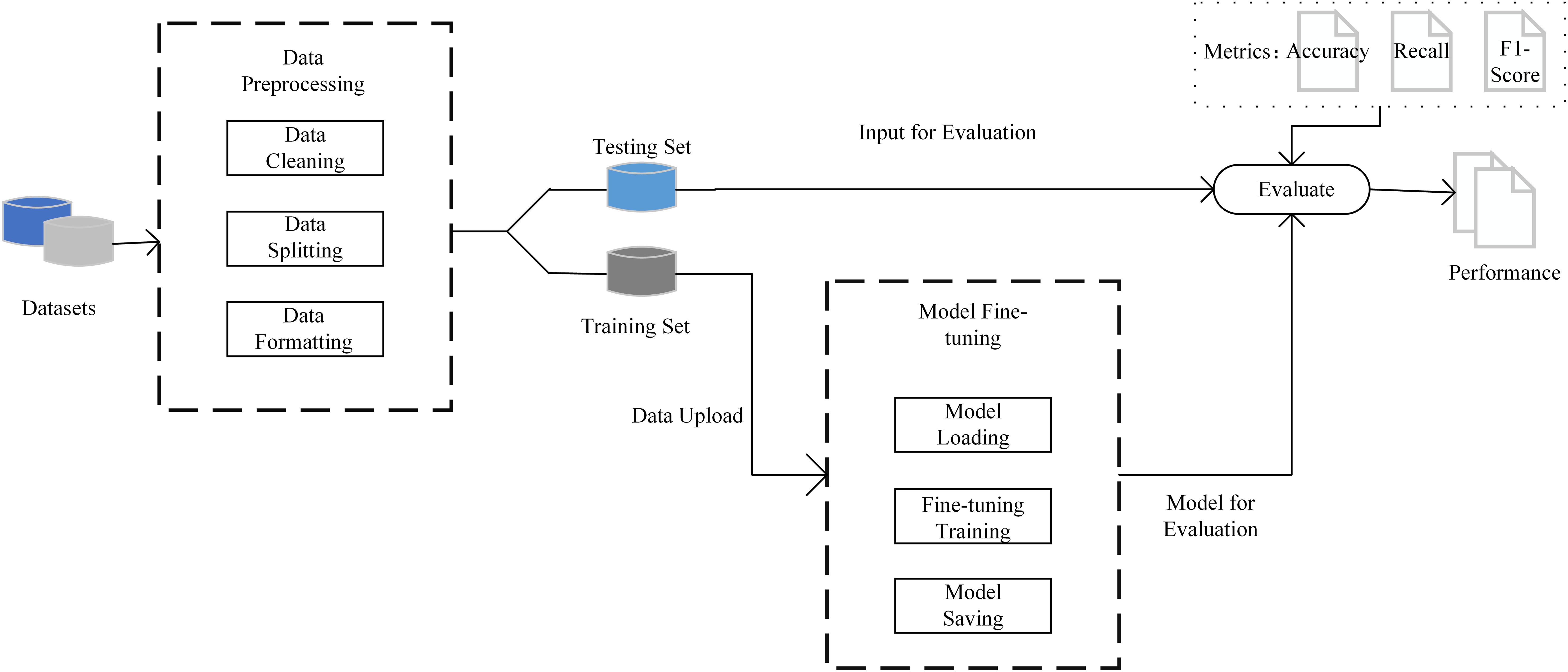
The model training process is based on the 10-fold cross-validation method. The dataset is divided into 10 subsets. In each round of training, nine subsets are selected as training sets, and the remaining one subset is used for testing. By repeating this process 10 times, it is ensured that each piece of data is validated as part of the test set and the training set, thereby minimizing the bias of data partitioning on the evaluation results. The fine-tuning process is performed through OpenAI’s application programming interface (API), and the model training is completed with the default parameter configuration without additional parameter tuning. After training, the test set is input into the fine-tuned model to generate sentiment prediction labels, and the classification performance of the model is evaluated, using indicators including precision, recall, and F1-score. As shown in Fig. 1, the flowchart of our proposed method.
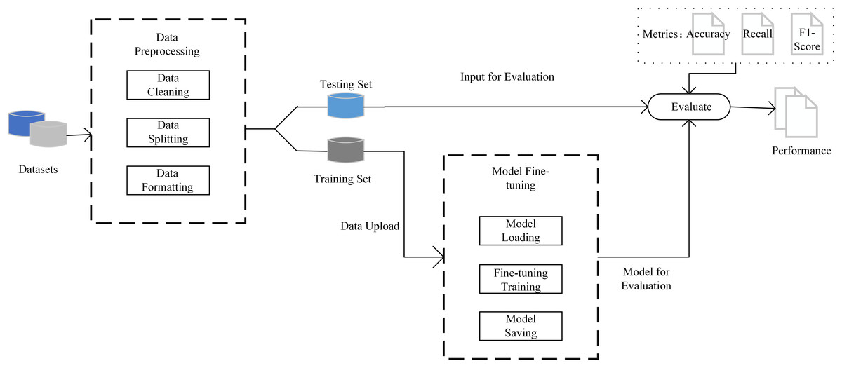
Figure 1: The process of proposed method.
Experimental setup
In order to verify the effectiveness of the fine-tuned GPT model in the SATD sentiment analysis task, the following two research questions were designed:
RQ1 (feature-based machine learning (ML) comparison): to what extent does fine-tuning GPT-3.5-turbo improve sentiment classification performance compared to traditional ML methods that rely on handcrafted Term Frequency–Inverse Document Frequency (TF-IDF) features (e.g., SVM, random forest, logistic regression, Naive Bayes, K-nearest neighbor (KNN))?
RQ2 (end-to-end deep learning comparison): how does GPT-3.5-turbo compare to end-to-end trained neural architectures (CNN, LSTM, Transformer) that learn embeddings and context from scratch without generative pre-training?
While both questions employ our 10-fold cross-validation scheme and evaluation metrics (precision, recall, F1), RQ1 highlights the benefits of large-scale language model pre-training over shallow feature engineering baselines, while RQ2 measures the benefits of GPT over similar deep learning models that already capture contextual patterns but lack the scale of pre-training.
Dataset
The dataset used in this study is from the public dataset provided by Fucci et al. (2021). This dataset is an extension and re-analysis of the original dataset released by Maldonado & Shihab (2015). The dataset is 4,071 SATD annotations extracted from 10 open source Java projects. Fucci et al. (2021) removed duplicates from the dataset on this basis, and finally retained 3,289 annotations, from which 1,038 were randomly selected for detailed manual analysis and expansion.
The extended dataset adopts a new classification system to classify the content of SATD in a more fine-grained manner and proposes a classification method with nine top-level categories and 32 subcategories. These categories cover various types such as functional issues, poor implementation choices, unfinished features, waiting events, documentation issues, and testing issues, thereby more comprehensively describing the content characteristics of technical debt reviews. As shown in Table 1, the complete categories and subcategories are shown. In addition, the dataset performs sentiment annotation on each annotation, and divides the sentiment tendency into three categories: negative, non-negative, and mixed, which further reveals the emotional state of developers when recording technical debt. To facilitate an intuitive understanding of the distribution of sentiments, Table 2 shows the specific distribution of different sentiment categories in the dataset, including the number and proportion of each sentiment category. At the same time, the dataset also extracts information such as class name, method name, BUG ID, URL and date contained in the comments, aiming to support the study of the patterns, sentiment tendencies and priority decisions of technical debt records. To further illustrate the emotional categories used in our sentiment analysis, we provide representative examples for the major sentiment types. For instance, a negative SATD comment such as:
“// FIXME: Is ‘No Namespace is Empty Namespace’ really OK?”
expresses dissatisfaction and questioning of correctness.
A mixed sentiment comment might be:
“// pattern now holds ** while string is not exhausted // this will generate false positives but we can live with that.”
which reflects a negative technical assessment combined with an accepting or tolerant tone.
As shown in Table 2, the dataset also includes a small number of samples under the exclude and no agreement categories. These require further clarification. The exclude category refers to comments that lack clear sentiment indicators or are ambiguous in interpretation. For example:
“// TODO: This isn’t an exact port of MRI’s pipe behavior, so revisit.”
The no agreement category corresponds to cases where human annotators could not reach a consistent labeling decision, such as:
“//TODO: is there a more elegant way than downcasting?”
Both of these categories were removed during data preprocessing to ensure training data quality.
| Top-level category | Sub-categories |
|---|---|
| Functional issues | Bug, Bad input validation, Unexpected behavior, Compatibility issue |
| Poor implementation choices | Code smell, Inefficient algorithm, Poor API usage, Hardcoding, Memory leak, Poor exception handling, Redundant/Duplicate code |
| Waiting/On-hold | Waiting on external dependency, Waiting on library update, Waiting for review, Waiting on design |
| Deployment issues | Build script issue, Environment configuration issue, Deployment pipeline failure |
| Outdated SATD comments | Comment not removed after fix, Stale comment |
| Partially/Not implemented functionality | Stub function, TODO placeholder, Temporary workaround |
| Testing issues | Missing test, Flaky test, Low test coverage |
| Documentation issues | Missing comment, Inaccurate documentation, Out-of-date README/Guide |
| Misalignment | Implementation–design mismatch, Requirements drift, Architectural inconsistency |
| Sentiment category | Count (#) | Percentage (%) |
|---|---|---|
| Non-negative | 714 | 68.79% |
| Negative | 304 | 29.29% |
| Mixed | 15 | 1.45% |
| Exclude | 3 | 0.29% |
| No agreement | 2 | 0.19% |
Evaluation indicators
To comprehensively evaluate the classification performance of the model in the sentiment analysis task, this study compared the model’s prediction results with the true labels and calculated the following three evaluation indicators:
Among them, true positive (TP) represents the number of samples correctly predicted as a certain type of sentiment, false positive (FP) represents the number of samples incorrectly predicted as a certain type of sentiment, and false negative (FN) represents the number of samples that actually belong to a certain type of sentiment but are incorrectly predicted as other categories. Precision represents the proportion of samples that actually belong to a certain category among all samples predicted as a certain type of sentiment, which is used to measure the accuracy of model prediction. Recall represents the proportion of samples that are correctly predicted as a certain category among samples that actually belong to a certain type of sentiment, which is used to measure the model’s ability to capture the sentiments of that category. F1-score is the harmonic mean of precision and recall, which is used to comprehensively evaluate the accuracy and coverage of the model. The higher the scores of these three indicators, the better the classification performance of the model.
In order to deal with the problem of imbalanced category distribution, the experiment uses weighted precision, recall and F1-score as evaluation indicators. In the specific calculation formula, the weights are allocated according to the actual number of samples in each category to reduce the impact of category imbalance on result evaluation.
Baseline models
(1) Traditional machine learning models
In order to evaluate the proposed method, five common traditional machine learning models were selected as benchmarks, namely logistic regression (LR), random forest (RF), support vector machine (SVM), Naive Bayes (NB) and K-nearest neighbor (KNN). LR, as an efficient supervised learning method, uses word frequency information to predict sentiment probability in this task, but has limitations in modeling complex nonlinear decision boundaries. RF, by integrating multiple decision trees for voting, can model nonlinear relationships and is robust to overfitting, but may not be as good as specialized sequence models at capturing long-distance context. SVM, as a powerful benchmark for text classification, is particularly good at processing high-dimensional sparse space using TF-IDF features, but its performance depends on the careful selection of kernel functions and regularization parameters. NB is a probabilistic classifier based on the assumption of feature independence, and is efficient in tasks where sentiment is strongly related to specific words. KNN, as a non-parametric method, classifies by comparing the labels of samples with those of neighboring points. The method is intuitive, but it is susceptible to the “curse of dimensionality” and noise in high-dimensional sparse text space.
(2) Deep learning models
To further explore more complex feature representations, we also selected convolutional neural networks (CNNs), long short-term memory networks (LSTMs), and Transformers as deep learning benchmarks. CNNs extract local features with sentimental meaning (such as keywords) from word vectors through convolution operations, and are good at identifying local patterns, but their limited receptive field makes it difficult to model long-distance dependencies. In contrast, LSTMs, as recurrent neural networks, can maintain and update memories with their gating mechanism, effectively tracking the sentiment context of the entire comment, and are particularly suitable for processing sentiment clues in long or complex sentences. Finally, the core of the Transformer model is the self-attention mechanism, which can directly model the relationship between any words in the sequence to capture global dependencies, and incorporate word order information through explicit positional encoding, which is particularly effective for understanding suggestive sentiment expressions that are distributed throughout the text or require complex logical inferences.
Data preprocessing
In the preprocessing process of all models, the original data was first cleaned and samples marked as mixed, exclude, and no agreement were removed. These samples are small in number and have unclear emotional tendencies, which cannot provide effective learning signals for the model, so they are removed.
For traditional machine learning models, LabelEncoder is first used to encode emotional labels and convert text categories (such as positive and negative) into numerical representations. The labels of the training set are encoded by fit_transform, and the test set is processed by the transform method to ensure consistency between the two. The TF-IDF vectorization method (TfidfVectorizer) is then used to convert the text data into a sparse feature matrix. The parameters set include a maximum number of features of 5,000 (max_features = 5,000), removal of stop words (stop_words = ‘english’), and unigrams and bigrams (ngram_range = (1, 2)) to capture the semantic information of words and phrases. This vectorization operation processes the training set and the test set separately to generate high-dimensional feature representations suitable for machine learning models.
In the deep learning model, text data is tokenized by Tokenizer, and the vocabulary is built by fit_on_texts. The text is then converted into integer sequences and the length is unified by pad_sequences (the maximum sequence length is 100). The vocabulary size is limited to 5,000 to balance feature richness and computational efficiency. Sentiment labels are binary processed, comparing the equality of text labels with “negative” to generate binary labels (0 and 1), and converted to one-hot encoding by to_categorical to fit the output layer of the classification model.
After the above steps, the text data is converted into a numerical matrix and the labels are converted into one-hot encoding, providing a unified and efficient input format for subsequent model training. These preprocessing processes are repeated in each fold cross validation to ensure the independence and consistency of data processing.
Parameter settings
(1) Machine learning model parameter settings
In the multinomial Naive Bayes model, the smoothing parameter alpha is set to the default value of 1.0, and the feature extraction range is unigram and binary n-gram. The regularization strength C of the logistic regression model is set to 1.0, the optimization algorithm is lbfgs, and the maximum number of iterations is set to 1,000 to ensure convergence on sparse data sets. At the same time, the random seed is set to 42 to ensure the reproducibility of the experimental results. In the random forest model, the number of decision trees is set to 100, the splitting criterion is Gini impurity, the maximum tree depth is not limited, and the minimum number of samples required for node splitting uses the default value of 2. In addition, the stability of the experimental results is ensured by setting the random seed to 42. The support vector machine model uses a linear kernel function and enables the probability estimation function. The regularization parameter C is set to 1.0 and the random seed is also set to 42. In the K-nearest neighbor model, the number of neighbors is set to 5, the distance metric uses the Euclidean distance, and the weight distribution is uniform weight.
All models are evaluated by 10-fold cross validation, and the average precision, recall, and F1-scores are reported to comprehensively measure the model performance.
(2) Deep learning model parameters
The CNN model receives a text sequence of fixed length as input and maps the text into a 128-dimensional vector representation through an embedding layer. Subsequently, the model uses three one-dimensional convolutional layers with kernel sizes of 2, 3, and 4, each containing 128 filters and an activation function of rectified linear unit (ReLU). The convolution operation is followed by a global maximum pooling layer to reduce the dimension of features and retain key information. The pooled features are concatenated and input into a 128-unit fully connected layer (ReLU activation), and are regularized by a dropout layer with a dropout rate of 0.5. Finally, a softmax layer with two classification nodes is used to complete the classification task.
The LSTM model captures text context information through a bidirectional long short-term memory network (Bidirectional LSTM). The input text is first mapped to a 128-dimensional vector through an embedding layer, and then passed to a bidirectional LSTM layer with 256 units. This layer is configured with dropout and recurrent dropout parameters (both are 0.2) to reduce overfitting and enhance model robustness. Subsequently, the feature vector passes through a 128-unit fully connected layer (ReLU activation), and is further regularized by a Dropout layer with a dropout rate of 0.5, and finally outputs the sentiment category probability distribution through a softmax layer of two classification nodes.
The Transformer model uses global feature extraction and a high-dimensional fully connected network to complete the classification task. The text sequence is mapped to a 120-dimensional vector representation through an embedding layer, and then the global features of the sequence are extracted through a global average pooling layer. The pooled features are sequentially passed through two fully connected layers with 1,024 units (ReLU activation), and a Dropout layer with a dropout rate of 0.5 is inserted between the layers for regularization, and finally the sentiment classification task is completed through a softmax layer of two classification nodes.
All deep learning models use the Adam optimizer with a learning rate of 0.001. The objective function is the categorical cross entropy loss function, which is used to minimize the deviation between the model prediction results and the true labels.
Results
Analysis for RQ1
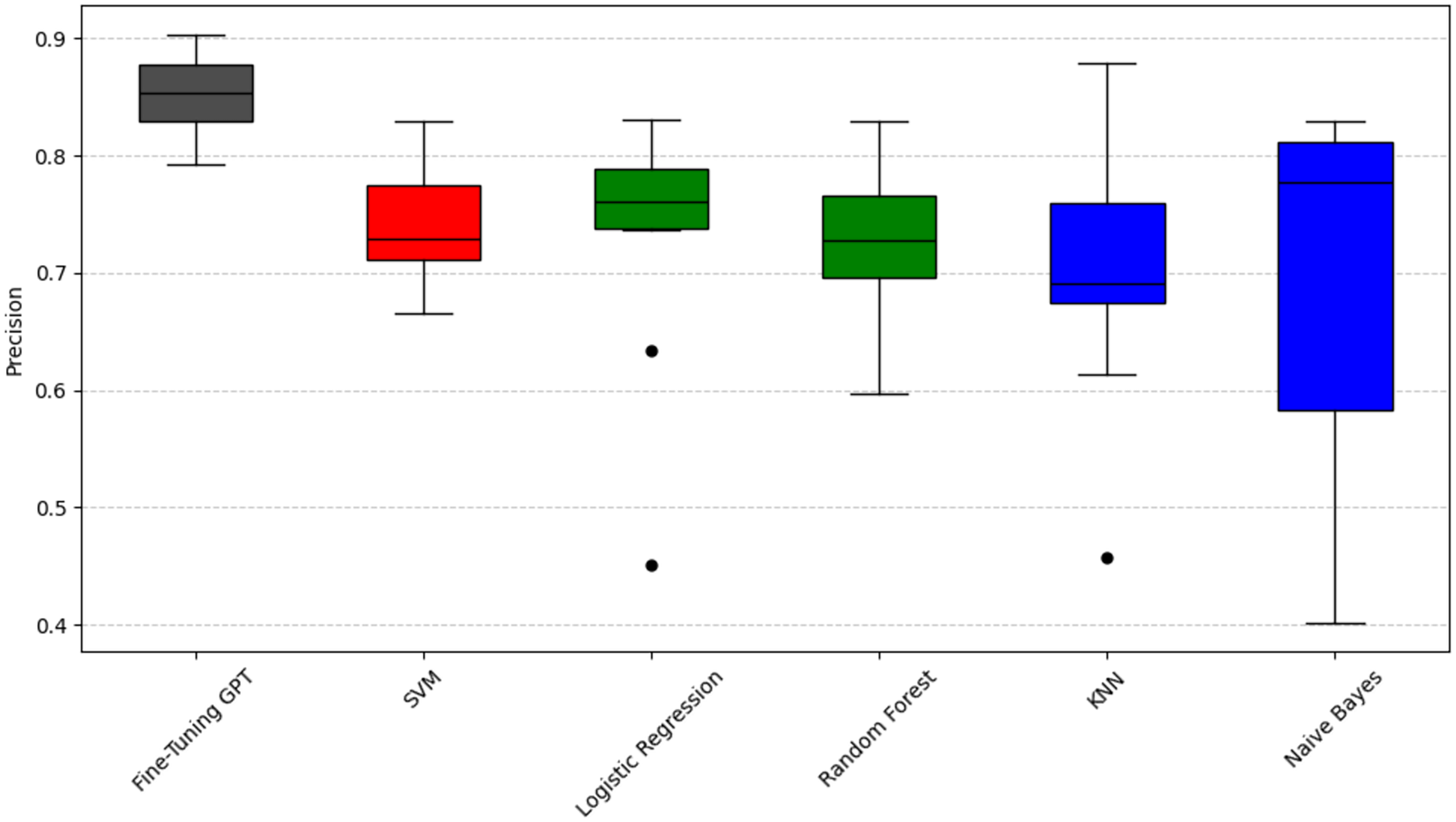
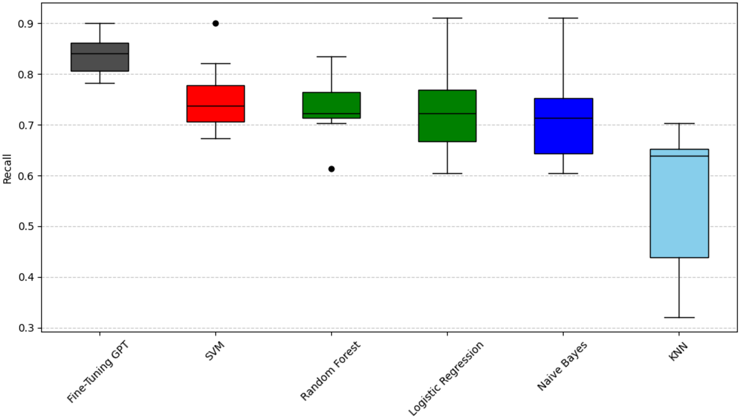
We use the Scott-Knott effect size difference (ESD) test (Jelihovschi, Faria & Allaman, 2014) to group all methods into statistically distinct classes based on their performance metric (precision, F1-score, or recall). This process recursively groups the techniques, maximizing the variance between groups at each split (p < 0.05). The “ESD” part of the test helps identify and mitigate the impact of significant outliers, ensuring that the ranking reflects true performance differences. Therefore, methods in the same color-coded group are not statistically significantly different, while methods in different color groups are significantly different. The groups are ranked by their average performance, with black representing the highest performing group, followed by red, then green, and finally blue or light blue representing lower performing groups. It is important to note that this clustering is done independently for each performance metric. As can be seen in Figs. 2, 3, and 4, fine-tuning GPT consistently outperforms all traditional machine learning models by a significant margin. Its average performance dominates the black group in all significant groupings for all three metrics, fully reflecting its excellent and statistically superior performance. The consistently strong performance of the fine-tuned GPT-3.5-turbo may be related to its complex Transformer architecture, extensive pre-training, and task-specific fine-tuning, which are expected to enhance its ability to capture complex semantic nuances critical to SATD sentiment prediction. However, this remains a plausible interpretation rather than a definitive conclusion, as further experiments such as ablation studies would be required to confirm the precise contributions of these factors.
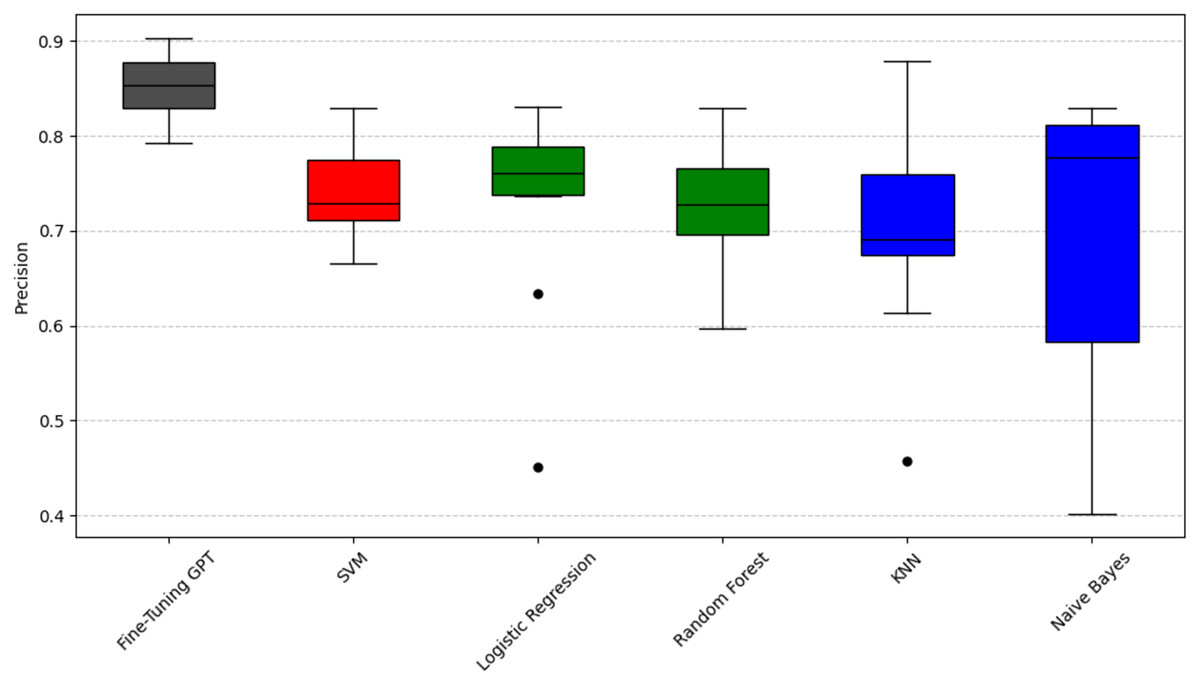
Figure 2: Scott-knott results of fine-tuning GPT vs. machine learning on indicator precision.
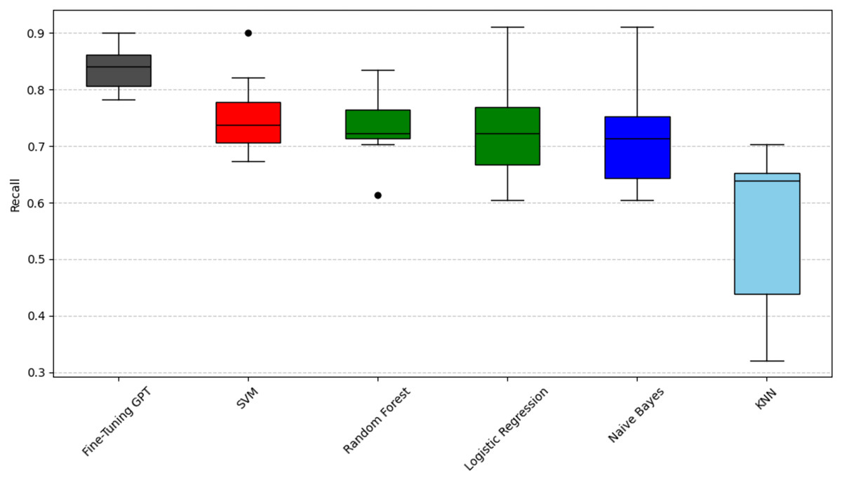
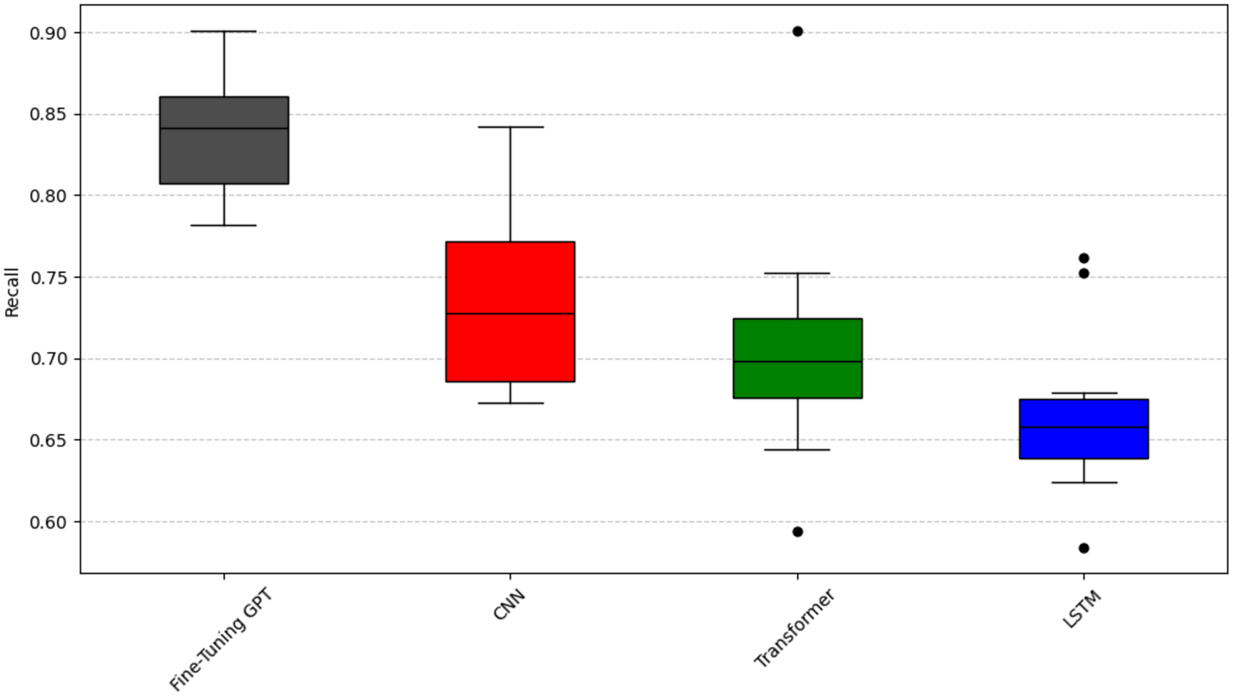
Figure 3: Scott-knott results of fine-tuning GPT vs. machine learning on indicator recall.
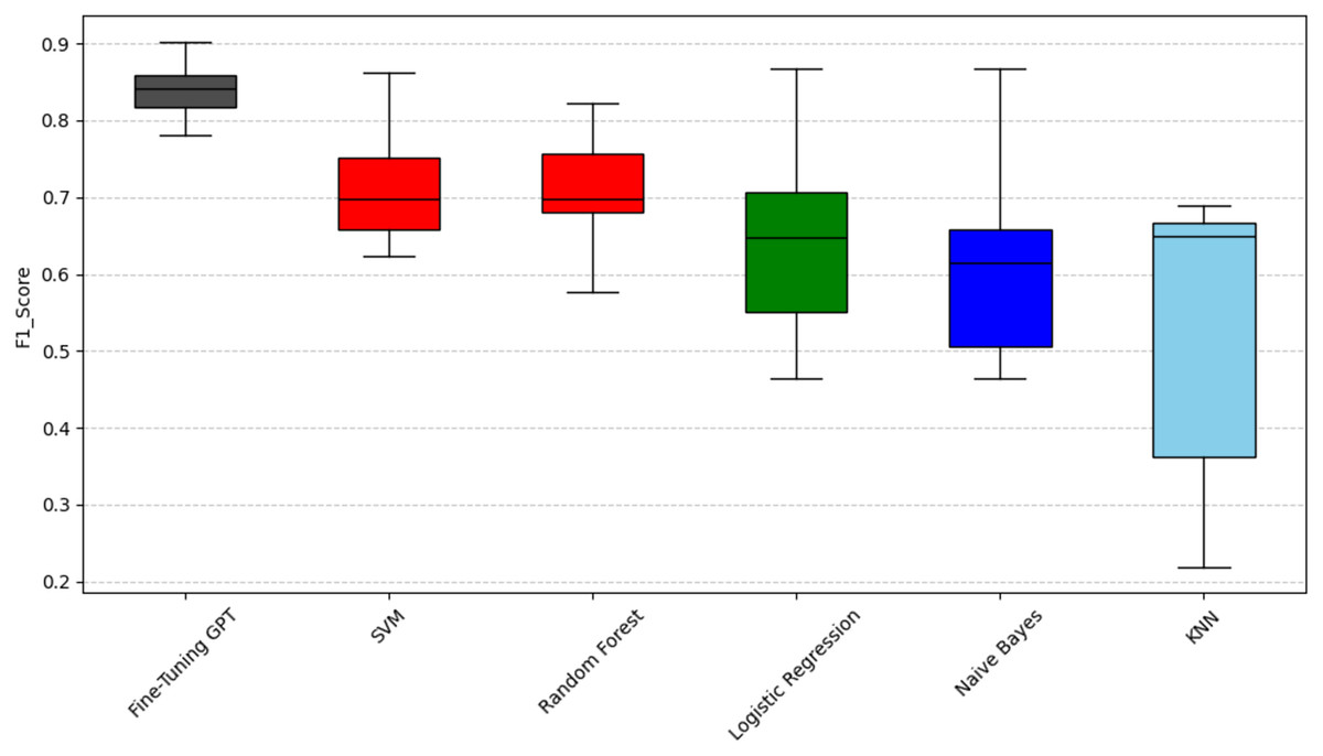
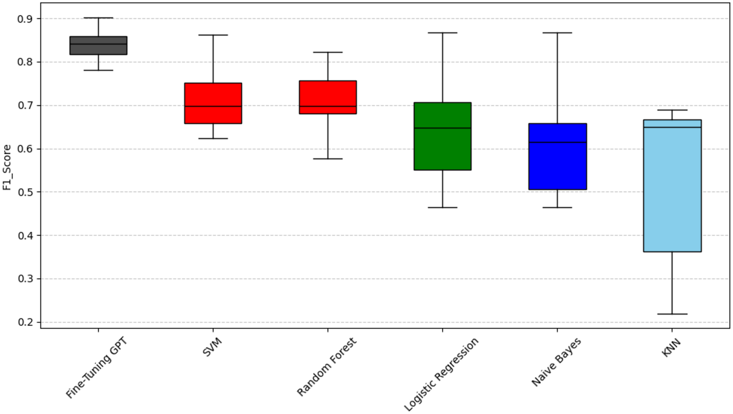
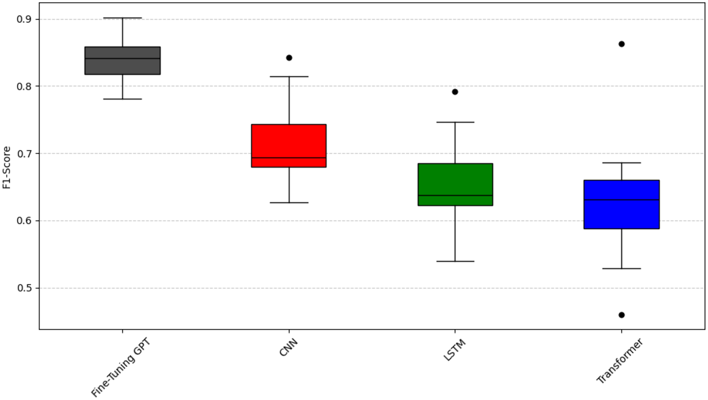
Figure 4: Scott-knott results of fine-tuning GPT vs. machine learning on indicator F1-score.
Taking accuracy as an example (Fig. 2), fine-tuning GPT has a significantly higher accuracy distribution than other models and is only in the black group, with the most stable performance. Among traditional machine learning models, SVM has relatively high accuracy performance and is classified as the red group. The advantage of SVM may stem from its effectiveness in the high-dimensional space of sparse features typical of text data. Logistic regression and random forest have relatively close accuracy performance and are classified as the green group, slightly inferior to SVM, and have a slightly wider distribution range; their ensemble (random forest) or linear (logistic regression) properties may not fully capture complexity like SVM or GPT. KNN and Naive Bayes are classified as the blue group, respectively, and their performance gradually decreases. Naive Bayes has the widest distribution range, with its lower limit close to 0.4, indicating that its performance is the most unstable, which may be due to its strong feature independence assumption that is often violated in natural language. Taking recall as an example (Fig. 3), fine-tuned GPT is again grouped separately in black. Among traditional models, support vector machine (SVM) is in the red group. Random forest and logistic regression are in the green group. Naive Bayes and KNN are in the blue and light blue groups, respectively. It is worth noting that KNN’s recall performance (light blue group, mean 0.559) is in a lower statistical group than its precision performance (blue group, mean 0.698). The difference in color grouping of KNN on different metrics is due to the fact that clustering for each metric is performed independently. This highlights that KNN’s relative position among similar models varies depending on specific aspects of performance; in this case, its relatively weak ability to capture all true positives (recall) and its relatively weak ability to ensure that its positive predictions are correct (precision). Taking F1-score as an example (Fig. 4), Fine-tuned GPT is still in the black group. Among traditional machine learning models, SVM and random forests have similar F1-score performance and are both grouped in the red group. Logistic regression is grouped in the green group. Naive Bayes and KNN are in the blue and light blue groups, respectively, with KNN again showing the widest distribution and the lowest F1-score. The fact that SVM and random forest are in the red group in terms of F1-score indicates that they achieve a better balance of precision and recall on this particular metric than logistic regression, which is in the green group.
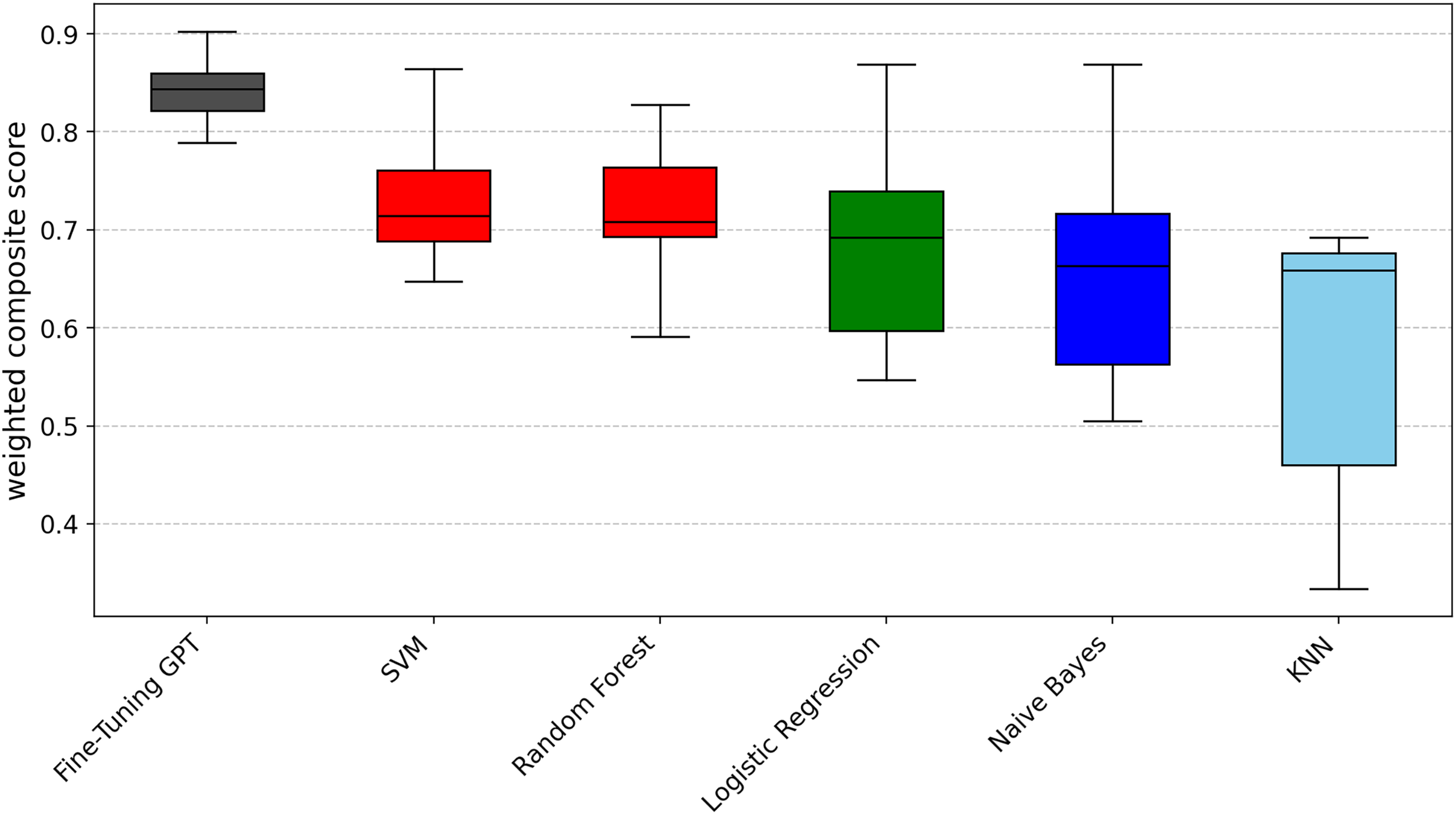
To provide a unified performance ranking for each metric of RQ1, we also calculated a weighted composite score for each technique (0.5 × F1-score + 0.25 × precision + 0.25 × recall). These composite scores were then subjected to the Scott-Knott ESD test. The results of the summary analysis, as shown in Fig. 5, largely confirm the findings of the individual indicators, where fine-tuning GPT still ranks at the top (black group), followed by SVM and random forest (red group), logistic regression (green group), Naive Bayes (blue group) and KNN (light blue group). This addresses the overall performance issue beyond the perspective of specific indicators.
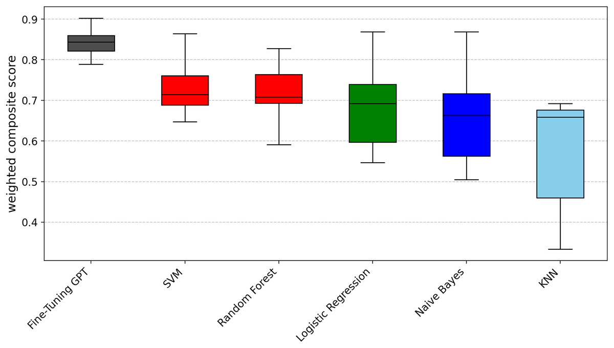
Figure 5: Scott-knott results of fine-tuning GPT vs. machine learning on indicator weighted composite score.
After completing the significant group analysis, the 10 folds in the cross-validation were analyzed separately as 10 independent data subsets to conduct a detailed performance comparison between fine-tuning GPT and five traditional baseline models. Through the precision, F1-score and recall metrics, we calculated the performance of each fine-tuning GPT and baseline model, and counted the number of wins (Win), draws (Draw) and losses (Loss), thereby obtaining the win-loss ratio (W/D/L) results. These results are listed in Tables 3, 4 and 5, respectively.
| Rounds | Fine-tuning GPT | Logistic Regression | Random forest | SVM | KNN | Naive Bayes |
|---|---|---|---|---|---|---|
| 1 | 0.848 | 0.762 | 0.597 | 0.773 | 0.613 | 0.762 |
| 2 | 0.884 | 0.830 | 0.817 | 0.829 | 0.879 | 0.830 |
| 3 | 0.792 | 0.786 | 0.677 | 0.710 | 0.717 | 0.815 |
| 4 | 0.859 | 0.737 | 0.691 | 0.744 | 0.686 | 0.793 |
| 5 | 0.903 | 0.759 | 0.715 | 0.715 | 0.680 | 0.802 |
| 6 | 0.858 | 0.741 | 0.773 | 0.821 | 0.774 | 0.566 |
| 7 | 0.824 | 0.634 | 0.709 | 0.713 | 0.458 | 0.634 |
| 8 | 0.802 | 0.451 | 0.741 | 0.702 | 0.695 | 0.453 |
| 9 | 0.850 | 0.789 | 0.747 | 0.665 | 0.672 | 0.402 |
| 10 | 0.890 | 0.831 | 0.830 | 0.775 | 0.809 | 0.815 |
| Average | 0.851 | 0.732 | 0.730 | 0.745 | 0.698 | 0.687 |
| W/D/L | – | 10/0/0 | 10/0/0 | 10/0/0 | 10/0/0 | 9/0/1 |
| Rounds | Fine-tuning GPT | Logistic regression | Random forest | SVM | KNN | Naive Bayes |
|---|---|---|---|---|---|---|
| 1 | 0.832 | 0.604 | 0.614 | 0.703 | 0.426 | 0.604 |
| 2 | 0.782 | 0.911 | 0.772 | 0.901 | 0.475 | 0.911 |
| 3 | 0.802 | 0.772 | 0.713 | 0.743 | 0.653 | 0.752 |
| 4 | 0.861 | 0.713 | 0.713 | 0.743 | 0.703 | 0.703 |
| 5 | 0.901 | 0.733 | 0.733 | 0.733 | 0.634 | 0.723 |
| 6 | 0.861 | 0.762 | 0.792 | 0.822 | 0.644 | 0.752 |
| 7 | 0.822 | 0.614 | 0.703 | 0.693 | 0.396 | 0.614 |
| 8 | 0.782 | 0.663 | 0.743 | 0.713 | 0.653 | 0.673 |
| 9 | 0.851 | 0.683 | 0.713 | 0.673 | 0.683 | 0.634 |
| 10 | 0.872 | 0.78 | 0.835 | 0.789 | 0.321 | 0.752 |
| Average | 0.837 | 0.724 | 0.733 | 0.751 | 0.559 | 0.712 |
| W/D/L | – | 9/0/1 | 10/0/0 | 9/0/1 | 10/0/0 | 9/0/1 |
| Rounds | Fine-tuning GPT | Logistic regression | Random forest | SVM | KNN | Naive Bayes |
|---|---|---|---|---|---|---|
| 1 | 0.833 | 0.465 | 0.576 | 0.654 | 0.291 | 0.465 |
| 2 | 0.821 | 0.868 | 0.794 | 0.863 | 0.572 | 0.868 |
| 3 | 0.781 | 0.714 | 0.686 | 0.709 | 0.672 | 0.664 |
| 4 | 0.859 | 0.632 | 0.683 | 0.700 | 0.690 | 0.598 |
| 5 | 0.902 | 0.663 | 0.714 | 0.697 | 0.647 | 0.632 |
| 6 | 0.859 | 0.684 | 0.770 | 0.795 | 0.668 | 0.646 |
| 7 | 0.817 | 0.493 | 0.679 | 0.655 | 0.241 | 0.493 |
| 8 | 0.787 | 0.537 | 0.709 | 0.665 | 0.664 | 0.542 |
| 9 | 0.850 | 0.594 | 0.663 | 0.624 | 0.652 | 0.492 |
| 10 | 0.876 | 0.716 | 0.823 | 0.766 | 0.219 | 0.662 |
| Average | 0.839 | 0.637 | 0.710 | 0.713 | 0.531 | 0.606 |
| W/D/L | – | 9/0/1 | 10/0/0 | 9/0/1 | 10/0/0 | 9/0/1 |
The “Average” row shows the average of all items. The “Win/Loss Ratio” row summarizes the number of projects where fine-tuning GPT outperforms, is equal to, or underperforms a specific baseline method. We find that fine-tuning GPT significantly outperforms all baseline models in terms of precision, recall, and F1-score. In terms of precision (Table 3), the average value of fine-tuning GPT is 0.851, which is significantly higher than 0.732 for logistic regression, 0.730 for random forest, 0.745 for SVM, 0.698 for KNN, and 0.687 for Naive Bayes. Compared with these baseline models, fine-tuning GPT’s performance improves by 16.3%, 16.6%, 14.2%, 21.9%, and 23.9%, respectively. According to the W/D/L analysis, fine-tuning GPT has an absolute advantage over the baseline models in all 10 compromises, except for logistic regression (9/0/1), and the results of other models are all 10/0/0. In terms of recall (Table 4), the average value of fine-tuning GPT is 0.837, which is significantly higher than 0.724 for logistic regression, 0.733 for random forest, 0.751 for SVM, 0.559 for KNN, and 0.712 for Naive Bayes, increasing by 15.6%, 14.2%, 11.5%, 49.7%, and 17.6%, respectively. W/D/L analysis shows that the scores of fine-tuning GPT for logistic regression, SVM, and Naive Bayes are 9/0/1, and for KNN and random forest are 10/0/0. In the F1-score indicator (Table 5), the average value of fine-tuning GPT reached 0.839, which is significantly higher than 0.637 of logistic regression, 0.710 of random forest, 0.713 of support vector machine, 0.531 of KNN and 0.606 of Naive Bayes, with an increase of 31.7%, 18.2%, 17.7%, 58.0% and 38.4% respectively. W/D/L analysis shows that fine-tuning GPT scores 9/0/1 against logistic regression, support vector machine and Naive Bayes, and scores 10/0/0 against KNN and random forest. Overall, compared with traditional machine learning models, fine-tuning GPT shows strong performance advantages and stability in all three indicators.
Analysis for RQ2
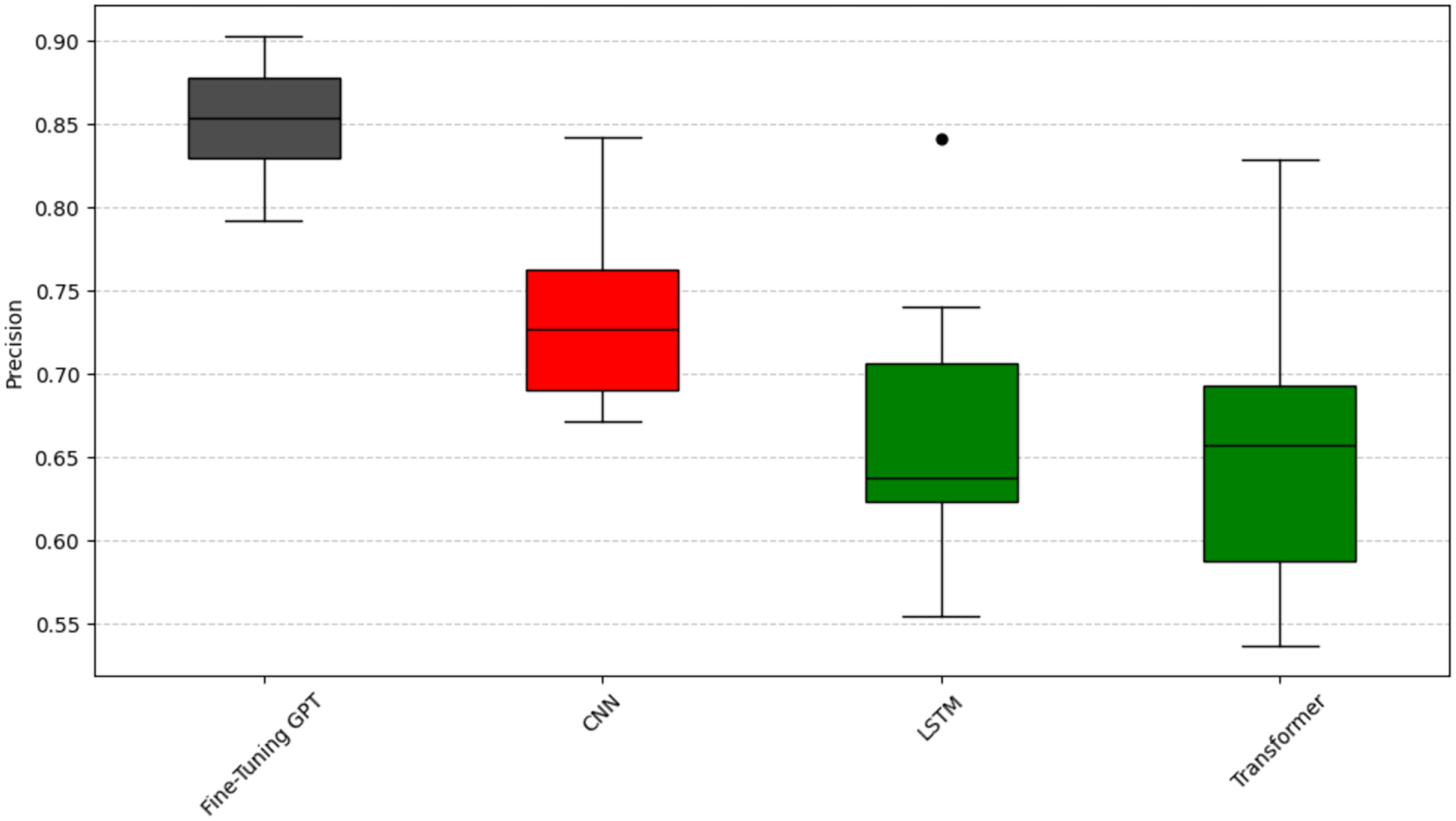
To analyze question RQ2, we compared the emotion capture ability of fine-tuning GPT with other deep learning models (CNN, LSTM, Transformer). The experiment again used the Scott-Knott ESD test and the same clustering logic and color scheme as question RQ1 (black represents the best performance, red, green, and blue represent the groups with poor performance) to significantly group the performance of these models. The results are shown in Figs. 6, 7, and 8. As can be seen from Figs. 6, 7, and 8, fine-tuning GPT always maintains a significant performance advantage among all compared deep learning models, and its average performance only occupies the share of the black group in the significant grouping, fully demonstrating its excellent performance. This continued advantage over other deep learning models highlights its advantage of large-scale pre-training combined with precise fine-tuning on the SATD emotion task.
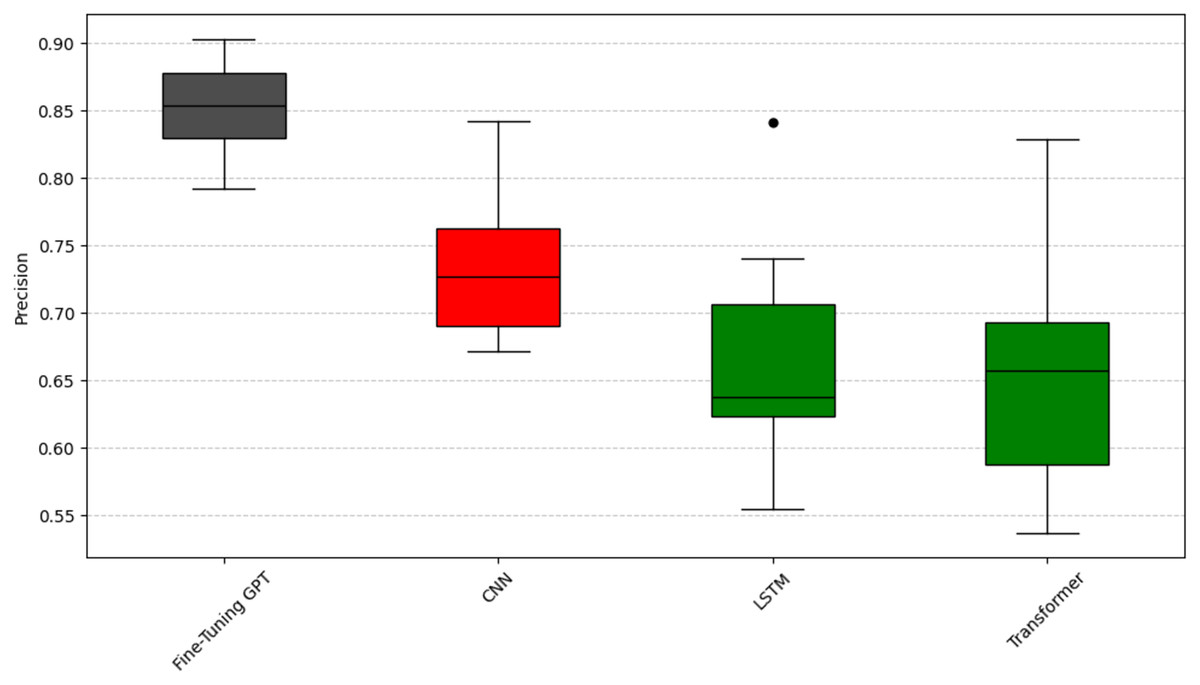
Figure 6: Scott-knott results of fine-tuning GPT vs. deep learning on indicator precision.
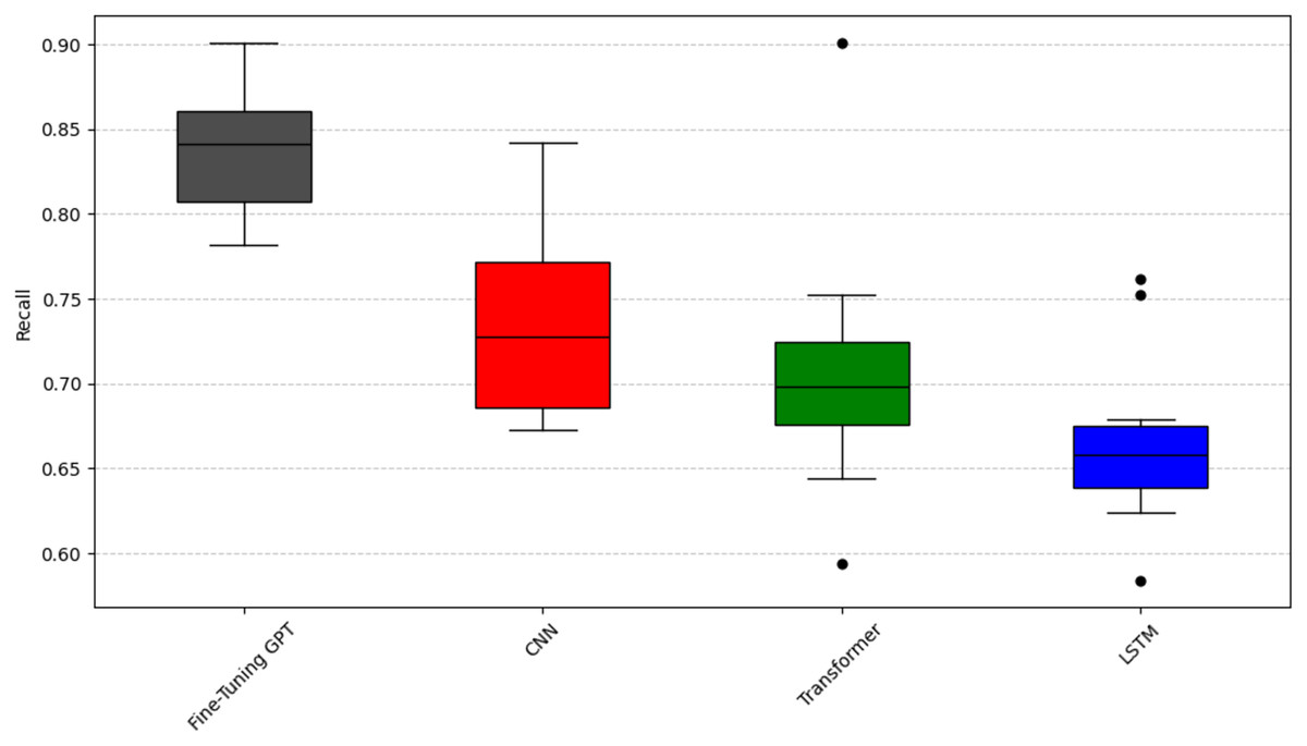
Figure 7: Scott-knott results of fine-tuning GPT vs. deep learning on indicator recall.
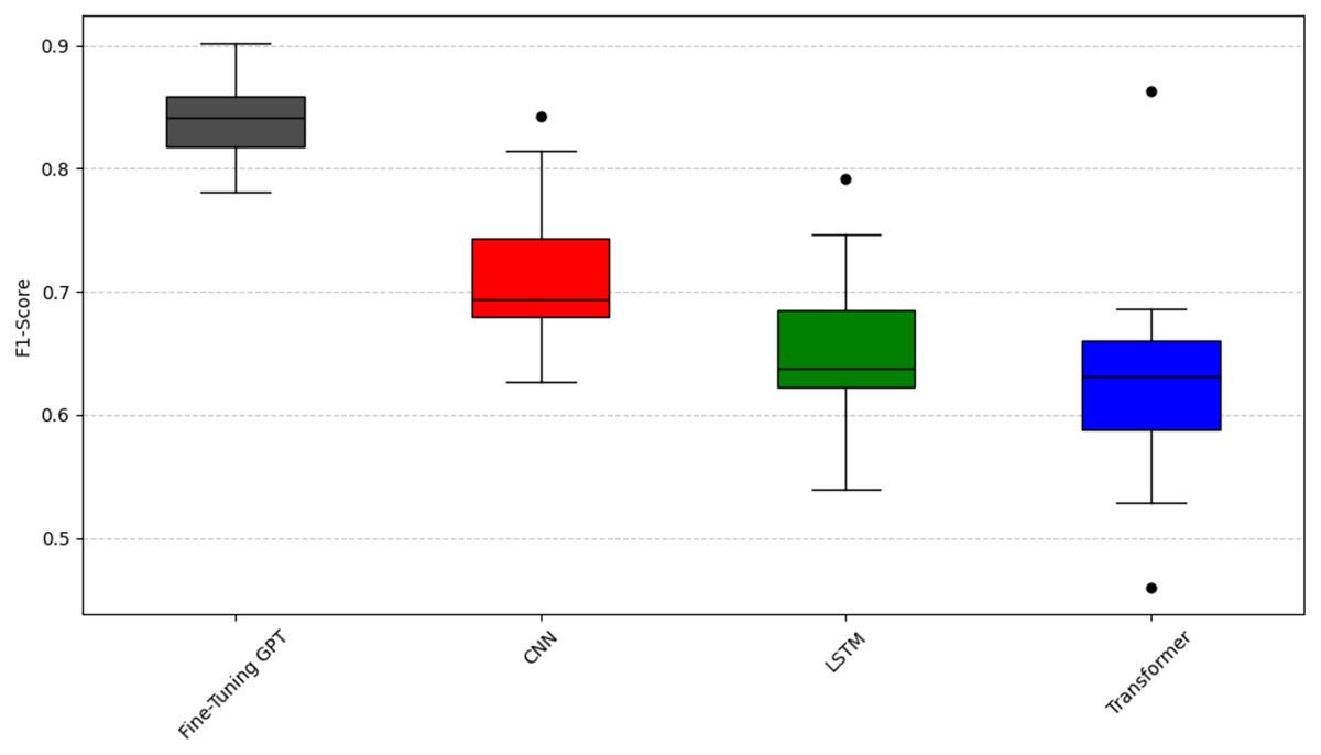
Figure 8: Scott-knott results of fine-tuning GPT vs. deep learning on indicator F1-score.
Taking the accuracy rate (Fig. 6) as an example, fine-tuning GPT is significantly higher than other models and is only in the black group, with a narrow distribution range and reliable performance. Among other deep learning models, CNN has a relatively high accuracy and is classified into the red group; CNN is known for effectively capturing local features, which is very useful for certain text patterns. LSTM and Transformer have low accuracy and are both classified into the green group. Taking the recall rate (Fig. 7) as an example, fine-tuning GPT is only in the black group. Among other deep learning models, CNN has a relatively high recall rate and is classified into the red group, but the distribution range is wide and there is a certain fluctuation. The recall rate of Transformer is slightly lower than that of CNN and is classified into the green group, and the distribution is relatively stable. LSTM has the worst recall performance and is classified into the blue group, and there are multiple obvious low value points, and the stability is poor. Taking the F1 value as an example (Fig. 8), fine-tuning GPT is completely in the black group and has a narrow distribution range. Among other deep learning models, CNN has a higher F1 value and is classified into the red group; LSTM has a slightly lower F1 value than CNN and is classified into the green group. Transformer has the most unstable F1 performance and is classified into the blue group, with a wide distribution and multiple outliers. The performance difference of the baseline Transformer model compared to fine-tuning GPT, which is also built on Transformer, highlights the key role of large-scale pre-training and targeted fine-tuning for fine-tuning GPT.
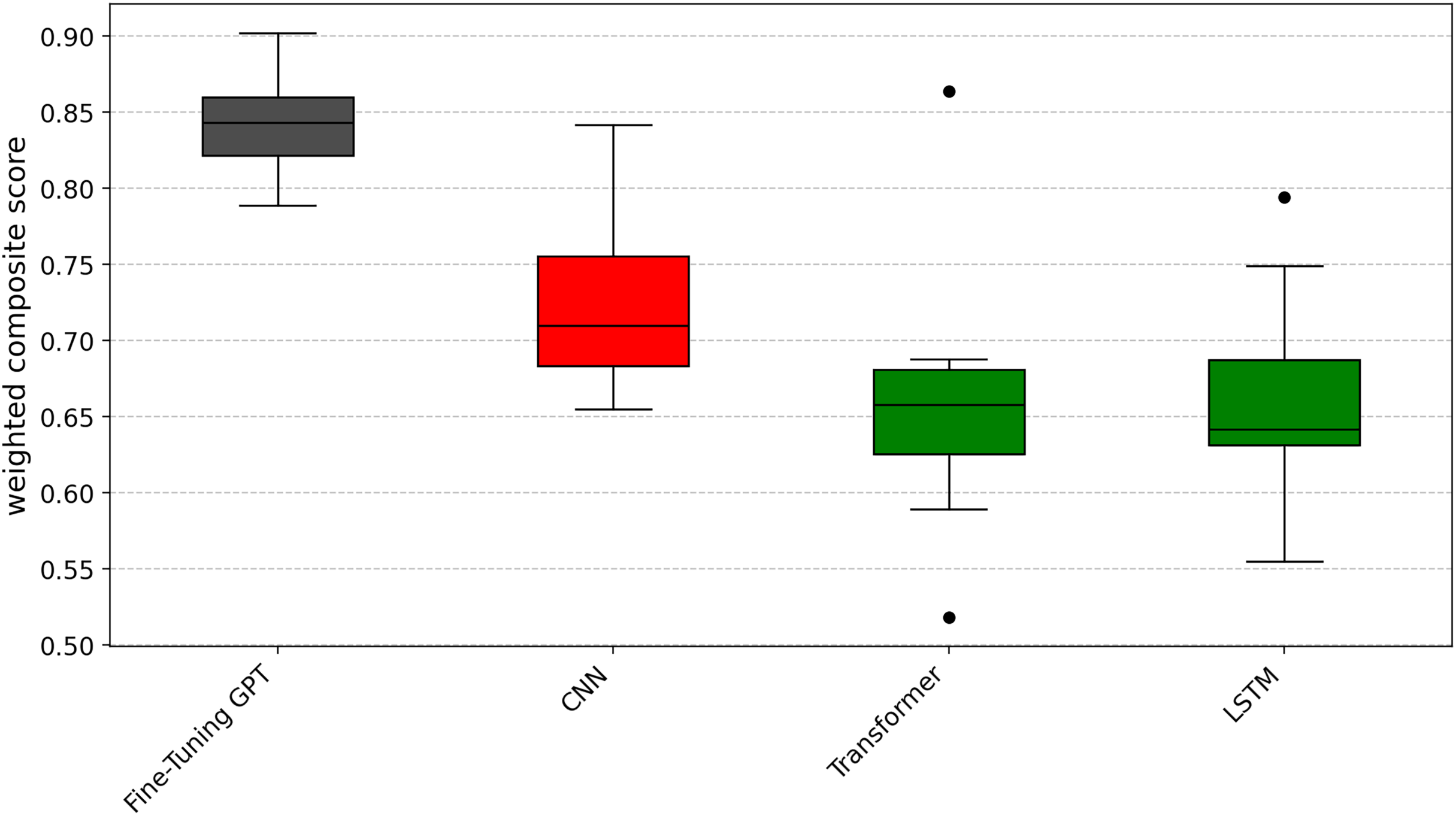
Similarly, in order to provide a unified performance ranking for each metric of RQ1, we also calculated the weighted composite score of each technology. Subsequently, as with RQ1, these composite scores were subjected to the Scott-Knott ESD test. The results are shown in Fig. 9, where fine-tuning GPT still ranks first (black group), followed by CNN (red group), Transformer (green group) and finally LSTM (green group).
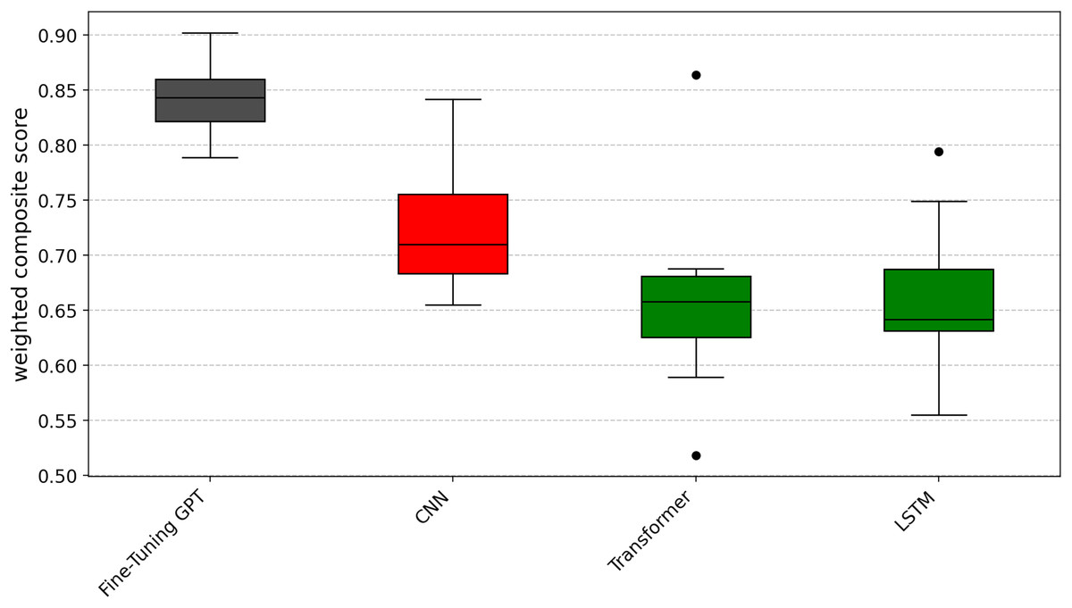
Figure 9: Scott-knott results of fine-tuning GPT vs. deep learning on indicator weighted composite score.
After completing the significant grouping analysis, we use the same W/D/L method as Question 1 to analyze the 10 folds in the cross-validation. The specific results are shown in Tables 6, 7, and 8. In terms of the precision indicator (Table 6), the average value of fine-tuning GPT is 0.851, which is significantly higher than CNN’s 0.737, LSTM’s 0.663, and Transformer’s 0.663, with improvements of 15.5%, 28.4%, and 28.4%, respectively. W/D/L analysis shows that fine-tuning GPT maintains a clear advantage (10/0/0) among all these deep learning models. In terms of the recall metric (Table 7), the average value of fine-tuning GPT is 0.837, which is significantly higher than CNN’s 0.740, LSTM’s 0.667, and Transformer’s 0.709, with increases of 13.1%, 25.5%, and 18.1%, respectively. W/D/L analysis shows that its scores for CNN and Transformer are 9/0/1, and for LSTM it is 10/0/0. In terms of the F1-score metric (Table 8), the average value of fine-tuning GPT is 0.839, which is significantly higher than CNN’s 0.715, LSTM’s 0.652, and Transformer’s 0.631, with increases of 17.3%, 28.7%, and 33.0%, respectively. The W/D/L analysis results show that fine-tuning GPT scores 9/0/1 with CNN and Transformer, and 10/0/0 with LSTM.
| Rounds | Fine-tuning GPT | CNN | LSTM | Transformer |
|---|---|---|---|---|
| 1 | 0.848 | 0.690 | 0.555 | 0.557 |
| 2 | 0.884 | 0.842 | 0.841 | 0.829 |
| 3 | 0.792 | 0.683 | 0.629 | 0.660 |
| 4 | 0.859 | 0.767 | 0.631 | 0.655 |
| 5 | 0.903 | 0.704 | 0.670 | 0.797 |
| 6 | 0.858 | 0.751 | 0.740 | 0.566 |
| 7 | 0.824 | 0.691 | 0.644 | 0.698 |
| 8 | 0.802 | 0.750 | 0.622 | 0.678 |
| 9 | 0.850 | 0.672 | 0.580 | 0.652 |
| 10 | 0.890 | 0.818 | 0.719 | 0.537 |
| Average | 0.851 | 0.737 | 0.663 | 0.663 |
| W/D/L | – | 10/0/0 | 10/0/0 | 10/0/0 |
| Rounds | Fine-tuning GPT | CNN | LSTM | Transformer |
|---|---|---|---|---|
| 1 | 0.832 | 0.693 | 0.584 | 0.594 |
| 2 | 0.782 | 0.842 | 0.752 | 0.901 |
| 3 | 0.802 | 0.683 | 0.663 | 0.723 |
| 4 | 0.861 | 0.772 | 0.634 | 0.673 |
| 5 | 0.901 | 0.723 | 0.653 | 0.713 |
| 6 | 0.861 | 0.772 | 0.762 | 0.752 |
| 7 | 0.822 | 0.673 | 0.653 | 0.683 |
| 8 | 0.782 | 0.733 | 0.663 | 0.683 |
| 9 | 0.851 | 0.683 | 0.624 | 0.644 |
| 10 | 0.872 | 0.826 | 0.679 | 0.725 |
| Average | 0.837 | 0.740 | 0.667 | 0.709 |
| W/D/L | – | 9/0/1 | 10/0/0 | 9/0/1 |
| Rounds | Fine-tuning GPT | CNN | LSTM | Transformer |
|---|---|---|---|---|
| 1 | 0.833 | 0.679 | 0.540 | 0.460 |
| 2 | 0.821 | 0.842 | 0.792 | 0.863 |
| 3 | 0.781 | 0.683 | 0.643 | 0.658 |
| 4 | 0.859 | 0.753 | 0.632 | 0.661 |
| 5 | 0.902 | 0.705 | 0.660 | 0.611 |
| 6 | 0.859 | 0.715 | 0.746 | 0.646 |
| 7 | 0.817 | 0.627 | 0.628 | 0.686 |
| 8 | 0.787 | 0.681 | 0.620 | 0.580 |
| 9 | 0.850 | 0.652 | 0.563 | 0.529 |
| 10 | 0.876 | 0.814 | 0.693 | 0.617 |
| Average | 0.839 | 0.715 | 0.652 | 0.631 |
| W/D/L | – | 9/0/1 | 10/0/0 | 9/0/1 |
By comparing RQ1 and RQ2, fine-tuning GPT shows significant performance advantages over traditional machine learning models and other deep learning models. Whether it is accuracy, recall or F1 score, fine-tuning GPT’s performance is always statistically significantly ahead of other models, and its stability in cross-validation is also excellent.
Discussion
This study aims to evaluate and compare the performance of fine-tuning GPT with various traditional machine learning models and other deep learning models for sentiment analysis of self-admitted technical debt (SATD) reviews. The results of both RQ1 and RQ2 clearly show that fine-tuning GPT (which is in the black group in the Scott-Knott ESD test) significantly outperforms all other evaluated models in terms of precision, recall, and F1-score metrics. It is important to note that this comparison focuses on a select set of traditional machine learning and deep learning baselines and does not include other LLM-based methods.
The continued strength of fine-tuning GPT can be attributed to several factors inherent in its architecture and training paradigm. Unlike traditional models that rely on often hand-crafted or relatively shallow features (e.g., TF-IDF for SVMs or word embeddings for simpler neural networks (NNs)), fine-tuning GPT leverages a deep Transformer architecture with an attention mechanism. This enables it to capture long-range dependencies and complex contextual nuances in text, which is critical for accurately interpreting sentiment in developer reviews that are often informal and domain-specific. Its extensive pre-training on a massive and diverse text corpus provides rich semantic understanding, which is then refined by fine-tuning on a specific SATD task. This is in stark contrast to the baseline Transformer model evaluated in RQ2. This model lacks the same scale of pre-training and specific fine-tuning as “fine-tuned GPT” and performs significantly worse (usually in the blue or green group), highlighting the key role of these two aspects. Among traditional machine learning models (RQ1), SVM (usually in the red group) generally performs best. This is consistent with the effectiveness of SVM in high-dimensional sparse feature spaces (usually text classification tasks using TF-IDF). However, its performance ceiling is still significantly lower than fine-tuned GPT. Models such as logistic regression and random forests (usually in the green group) provide reasonable baseline performance, but lack the ability to model complex interactions like support vector machines (SVM) (via kernel functions) or deep learning models. KNN and Naive Bayes (usually blue or light blue groups) struggle the most, likely because KNN suffers from high dimensionality issues and Naive Bayes’ strong feature independence assumption is often violated in natural language. CNNs (usually red groups) perform well compared to other deep learning models (RQ2), likely because they are able to effectively capture local n-gram patterns. LSTM and baseline Transformer (usually green or blue groups) are less efficient than fine-tuning GPT and CNN, suggesting that while they can model sequences, fine-tuning GPT’s specific architecture, pre-training size, and fine-tuning strategy give it a decisive advantage in this particular task.
The Scott-Knott ESD test provides clear statistical groupings for these techniques. Top models like fine-tuning GPT have consistent color groupings for most metrics, indicating robust and comprehensive performance. While models like KNN have slightly different colors for different metrics (e.g., blue for precision, light blue for recall), this highlights that their relative strengths and weaknesses vary depending on the evaluation dimension; testing is done on a per-metric basis, allowing for such detailed observations. Aggregate analysis using the combined score (Figs. 5, 9) further solidifies the overall ranking, confirms fine-tuning GPT’s leading position, and provides a comprehensive view of performance. The ESD portion of the test ensures that these groupings are robust to minor outliers in the performance scores. The different performance tiers (black, red, green, and blue) identified by Scott-Knott clustering have significant practical implications for managing spontaneous technical debt (SATD). In the highest-performing black group, the fine-tuned GPT model, with its superior accuracy and reliability, is a prime candidate for integration into automated systems (such as Continuous Integration/Continuous Deployment (CI/CD) pipelines or code review tools), providing high-confidence sentiment labels for developer comments, thereby helping to proactively identify and prioritize technical debt. Although the models in the red group (such as SVM in question 1 and CNN in question 2) are slightly inferior to the black group in statistical performance, they are robust secondary options and can be used as alternatives when the black group models are computationally resource-constrained or as reliable baselines; however, additional human supervision may be required for full automation. Models in the green group (such as logistic regression/random forest in RQ1 and LSTM/Transformer in RQ2) have moderate performance and should be used with caution in fully automatic SATD detection due to the high risk of misclassification. They are more suitable for assisting human annotators or performing preliminary analysis, where a certain degree of noise can be tolerated. As for models in the blue/light blue group (such as KNN/Naive Bayes in RQ1), they are generally not recommended for automatic SATD sentiment analysis due to their significant limitations in performing the task, as they are more prone to errors and may cause critical debts to be ignored or generate too many false positives. Therefore, by gaining a deeper understanding of these performance levels, development teams can make informed model deployment decisions based on their specific needs, available resources, and fault tolerance. For example, an organization that aims to maximize the automation and accuracy of SATD identification should prioritize investment in models in the black group.
Validity threats
This section discusses possible threats to the validity of our study and follows a widely adopted validity framework that includes construct validity, internal validity, external validity, and conclusion validity.
Construct validity
Construct validity refers to whether the methods and metrics used in the study accurately measure the intended concepts. Our study relies on the existing SATD dataset, which contains manually annotated sentiment labels. The inherent subjectivity of sentiment annotation may lead to inconsistencies or label biases. Although the dataset is carefully prepared and widely used in previous studies, some sentiment labels may not perfectly reflect the real emotional expressions of developers.
In addition, although we adopt widely accepted performance metrics—precision, recall, and F1-score—these metrics may not fully capture the actual impact of sentiment misclassification in software engineering settings. For example, misclassifying highly negative SATD reviews may incur greater operational costs than misclassifying neutral reviews, which is not explicitly simulated in this study.
We mitigate these risks by using cross-validation to provide more reliable performance estimates and choosing metrics commonly used in sentiment analysis and SATD research. Nonetheless, future studies may consider incorporating cost-sensitive evaluations or exploring more fine-grained, domain-specific sentiment taxonomies.
Internal validity
Internal validity focuses on whether the observed differences in model performance are truly attributable to the experimental intervention rather than confounding factors.
The baseline traditional machine learning and deep learning models in this study were implemented specifically for this experiment. While we used standard libraries (e.g., scikit-learn, PyTorch) and followed best practices and parameter settings reported in relevant studies, we acknowledge that these baseline implementations may not fully reflect the best performance of these methods in all cases. Due to computational limitations, exhaustive hyperparameter tuning was not performed for all baseline models, which may affect the fairness of the comparison. This poses a potential threat to validity.
We have made the full source code and experimental details publicly available so that other researchers can reproduce and improve these baselines.
We also mitigated another common internal validity threat by strictly distinguishing each set of training and test sets and ensuring that no data leakage occurred during the 10-fold cross-validation process.
External validity
External validity refers to the generalizability of our findings beyond the specific dataset and setting used in this study.
Our experiments were conducted on the SATD dataset from a single software project, which may limit the generalizability of our results to other domains, programming languages, or software ecosystems. Developers’ emotional expressions may vary across organizations, teams, or cultures, especially in multilingual settings. In addition, our fine-tuned GPT-3.5-turbo model is task-specific and its performance on SATD on other datasets remains to be verified.
We mitigated this threat by employing 10-fold cross-validation to ensure generalization within the dataset. However, future research should explore the application of this method on cross-project, cross-domain, and multilingual SATD datasets to verify the broader applicability of our findings. Furthermore, the exclusion of other LLM-based baselines (e.g., Code Bidirectional Encoder Representations from Transformers (CodeBERT)) limits direct comparisons with state-of-the-art methods in this field.
Conclusion validity
Conclusion validity refers to the appropriateness of the statistical methods used to support the conclusions of the study.
We applied the Scott-Knott ESD test to statistically compare the performance of different models, which is a well-established method for grouping and ranking classifiers under multiple evaluation settings. We also report the average performance metrics and win/tie/loss statistics across all evaluation settings. However, all statistical methods rely on underlying assumptions, so other nonparametric tests (e.g., Friedman and Nemenyi post hoc tests) may be considered in future studies to further validate the findings.
Conclusions
This article studies the SATD sentiment prediction problem in software development and proposes a method based on the GPT-3.5-turbo fine-tuning model. SATD is a form of developers explicitly recording technical compromises through comments, and analyzing its sentiment information is of great significance for technical debt management. An efficient sentiment analysis framework is built by fine-tuning the GPT-3.5-turbo model to adapt to the SATD sentiment prediction task. The experimental design uses 10-fold cross-validation and is systematically compared with traditional machine learning models and deep learning models to evaluate the precision, recall and F1-score indicators of the model. Experimental results show that the fine-tuning GPT-3.5-turbo model performs significantly better than traditional machine learning and deep learning models in sentiment analysis tasks. In terms of precision, the average value is 0.851, which is 14.2% higher than the best traditional machine learning model SVM; in terms of recall, the average value of fine-tuning GPT is 0.837, which is 11.5% higher than the best traditional machine learning model SVM; in terms of F1-score, the average value is 0.839, which is 17.3% higher than the best deep learning model CNN. These results prove that fine-tuning GPT not only has higher classification accuracy and recall ability in sentiment analysis tasks, but also shows superior overall performance and balance.
This study proposes a generative pre-training model framework for SATD sentiment prediction for the first time, verifying the unique potential of the GPT model in capturing complex sentiments. Through comprehensive experimental comparisons, the significant advantages of GPT in sentiment prediction tasks are revealed, providing new ideas and technical references for SATD management research. The experimental data, source code, and detailed instructions for reproducing the results of this study are publicly available at https://github.com/yangxingguang/satd_sentiment_GPT.
This code repository contains: (1) preprocessed SATD dataset for 10-fold cross-validation (train and test are provided in CSV and JSONL formats, respectively); (2) source code for fine-tuning GPT models (‘Fine-tuning GPT.py’), deep learning models (CNN, LSTM, Transformer in ‘Deep Learning.py’), and traditional machine learning models (e.g., SVM, Random Forest in ‘Machine Learning.py’); (3) a detailed ‘README.md’ file that details the project overview, prerequisites, data description, code explanation, and step-by-step experimental steps to reproduce our results.
This work also has practical relevance in software engineering. For example, in an issue tracking system, when developers’ comments show repeated negative sentiment (e.g., “//FIXME: This hack is scary, but necessary”), our model can flag these issues to help project managers identify potential technical debt risks or team bottlenecks. Similarly, sentiment trends in code review discussions can be tracked to assess team communication dynamics. By integrating this framework into the development workflow, teams can gain new insights into sentiment patterns related to project quality or delivery delays.
Moreover, this approach is relevant to modern technical debt management (TDM). As highlighted by Albuquerque et al. (2023), intelligent techniques such as machine learning and natural language processing (NLP) are increasingly used for debt detection, monitoring, and prioritization in TDM. Our model complements this trend by introducing developer sentiment as an auxiliary signal for technical debt awareness. For example, a cluster of negative SATD comments may indicate a fragile or problematic area of code. These insights provide additional value to technical managers who aim to proactively identify and mitigate debt-related risks.
In addition to detecting individual SATD comments with negative sentiment, the proposed sentiment prediction framework can also be integrated with issue tracking systems and software repository mining to support a more comprehensive software quality management workflow. Previous studies have shown that the sentiment and ranking of issue comments are closely related to issue resolution time and team productivity (Ortu et al., 2016; Mäntylä et al., 2016). Automatically identifying SATD sentiment trends over time can help project managers prioritize technical debt items that lead to growing developer frustration or recurring issues in unresolved issues. In addition, issue type classification and repository text mining have been shown to be effective in supporting software maintenance and project evaluation (Dobrzyński & Sosnowski, 2023; Herzig, Just & Zeller, 2013). By combining sentiment analysis with issue type classification, intelligent project dashboards can be developed that not only track the number of SATDs, but also display emotional comments associated with high-risk issue types (e.g., functional failures or blocking dependencies). This integration can provide valuable signals for proactively managing technical debt and improving team communication dynamics throughout the software development lifecycle.
Despite the positive results achieved in this study, several limitations remain, which are discussed in detail in ‘Validity Threats’, “Threats to Validity.” To address these limitations, future research directions include: expanding the dataset to cover cross-domain and multilingual SATD corpora; developing context-aware sentiment classification methods tailored to the semantics of technical debt; employing nonparametric hypothesis testing techniques for more rigorous statistical validation; and exploring domain adaptation techniques to enhance the ability of large language models to handle software engineering expertise. Furthermore, future research could further compare with other large language model (LLM)-based approaches, including alternative hint engineering strategies, contextual learning mechanisms, or newer versions of LLM fine-tuning models. While this comparison was not included in the current evaluation, such research is expected to provide deeper insights into the relative strengths and potential for improvement of LLM approaches in SATD sentiment classification. For example, comparative analysis with other LLM approaches, such as CodeBERT and BERT, would contribute to the construction of a more comprehensive SATD sentiment analysis benchmark.
Although current experimental results show that the fine-tuned GPT-3.5-turbo outperforms some traditional machine learning and deep learning baseline models, future work will prioritize expanding the scope of comparison to include more advanced LLM methods to more comprehensively evaluate its effectiveness and applicability.