
GRIFD: a graded region-wise dissection and cross-pooling RNN framework for precise diabetic retinopathy detection in fundus images
- Published
- Accepted
- Received
- Academic Editor
- Xiangjie Kong
- Subject Areas
- Artificial Intelligence, Computer Vision, Data Mining and Machine Learning, Data Science, Optimization Theory and Computation
- Keywords
- Local electricity market, Peer-to-peer energy trading, Artificial intelligence, Deep reinforcement learning, Fair value sharing, Energy efficiency
- Copyright
- © 2025 Alkharashi et al.
- Licence
- This is an open access article distributed under the terms of the Creative Commons Attribution License, which permits unrestricted use, distribution, reproduction and adaptation in any medium and for any purpose provided that it is properly attributed. For attribution, the original author(s), title, publication source (PeerJ Computer Science) and either DOI or URL of the article must be cited.
- Cite this article
- 2025. GRIFD: a graded region-wise dissection and cross-pooling RNN framework for precise diabetic retinopathy detection in fundus images. PeerJ Computer Science 11:e3197 https://doi.org/10.7717/peerj-cs.3197
Abstract
Early and precise detection of diabetic retinopathy (DR) is essential in averting vision impairment. This work introduces graded region wise inspection and feature dissection (GRIFD), a novel deep learning architecture designed explicitly for fine-grained DR detection from fundus images. GRIFD enforces a graded region of interest (ROI) dissection approach, which methodically segments fundus images into diagnostic blocks to promote local lesion visibility. A recurrent neural network (RNN) is used to model sequential dependencies between these ROI blocks, aiming to mimic the progressive development of DR symptoms. We also introduce a cross-pooling refinement procedure to eliminate inter-region inconsistencies and improve feature continuity. Experiments on the Mendeley and EyePACS benchmarks show that GRIFD obtains 94.35% accuracy, 96.05% precision, and 94.91% specificity on Mendeley, all of which surpass baseline models such as convolutional neural network (CNN), long short-term memory (LSTM), Transformer, and some published DR detection models. The introduced framework presents a lightweight and robust method for DR screening and can potentially facilitate real-time clinical practice.
Introduction
Diabetic retinopathy (DR) is a chronic disease resulting from dysfunction of insulin production in the retina. DR detection is a crucial task in healthcare applications (Ikram et al., 2024). Fundus photography is a process that captures the retina of the eye with a fundus camera. Fundus images are inputs that produce the exact condition of the retina. A feature extraction-based DR detection method is used in healthcare centers (Kaur, Mittal & Singla, 2022). The extraction technique extracts the infected regions and patterns of the regions from fundus images. The extracted features are used as datasets in further DR detection processes (Kumari et al., 2022). The extraction-based method identifies the blood vessels with infectious regions which eliminates the latency in detection (Jabbar et al., 2024b). The detection method maximises the precision ratio when providing medical services to patients. An automated DR detection approach using fundus images is used for the detection process (Abushawish et al., 2024). The detection approach analyses the textural features and factors of the retina via given fundus images. The approach is used as an early DR detection which improves the feasibility range of the detection systems (Alavee et al., 2024).
Region of interest (ROI) extraction is a process that extracts the important regions from the fundus images. ROI extraction reduces the data loss ratio while detecting DR disease (Bansal, Jain & Walia, 2024). A deep neural network (DNN) algorithm-enabled ROI extraction method is used for DR detection. The DNN algorithm inherits a classifier that classifies the exact types of diseases according to the condition of the retina (Muthusamy & Palani, 2024). The DNN algorithm analyses the significant factors that are extracted from the images. The extraction method is a two-stage method that identifies segments of the ROI as per necessity (Sundar & Sumathy, 2023). The method elevates the functional quality and capability level of the detection systems. An improved feature extraction technique is used for ROI extraction in DR detection. The extraction technique utilises a Gaussian mixture model (GMM), which identifies the lesion and surrounding regions in the input images. The GMM also examines the difference between features and patterns for further disease detection processes. The extraction technique enlarges the accuracy range of DR detection in healthcare applications (Berbar, 2022; Jabbar et al., 2024a). However, the majority of the existing approaches are plagued by persistent issues such as variable segmentation of lesion boundaries, weak adaptability to locale-based pixel variability, and excessively high rates of false-positive detection when vascular structures interfere with lesions. Furthermore, the typical feature extraction methods cannot model inter-regional dependencies and consequently exhibit inefficient performance in the presence of complex fundus image scenarios.
Machine learning (ML) algorithms are used in DR detection for the region dissection process. ML improves the precision level in the DR detection process (Pavithra, Jaladi & Tamilarasi, 2024). A hybrid inductive ML algorithm-based detection model is used for region dissection. The regions are segmented as per reliable data, which reduces the complexity level of the detection process (Aziz, Charoenlarpnopparut & Mahapakulchai, 2023). The ML algorithm pre-processes the data collected from the fundus images. The collected data is analysed using an extraction technique that minimises the energy consumption ratio in further detection processes (Malhi, Grewal & Pannu, 2023). The model segments the important regions of the images for detection. The ML algorithm-based model enhances the quality range of the detection process (Gupta, Thakur & Gupta, 2022). A convolutional neural network (CNN)-based region dissection method is also used for diabetic retinopathy (DR) detection. The CNN algorithm evaluates the visual representation of the fundus images and segments the regions according to the severity (Shamrat et al., 2024). The segmented regions are used as inputs, improving the precision level of DR detection. The CNN-based dissection method is used for early DR detection in healthcare systems (Niu et al., 2021). To overcome these shortcomings, we propose an innovative Graded Region-of-Interest Feature Dissection (GRIFD) framework that integrates sequential feature learning using a recurrent neural network (RNN) with a cross-pooling validation process. The innovative aspect of GRIFD lies in its ability to iteratively examine ROI distributions of pixels to identify spatial-sequence-based variation violations, as well as extract DR-related regions with higher precision and specificity by isolating these regions from one another. GRIFD differs from conventional methods by adaptively eliminating inconsistent features using a learned dissection technique, thereby improving resistance to lesion variability and illumination inconsistencies in the context of fundus images.
The article’s contributions are listed below:
-
To study different methods related to DR lesion segmentation using optimization and deep learning methods proposed by other authors in the past
-
To propose a novel graded region-of-interest feature dissection method to improve the dissection precision of DR lesions from fundus images
-
To validate the proposed method’s performance using accuracy, precision, specificity, mean error, and detection delay metrics
-
To verify the proposed method’s performance through a comparative analysis using the above metrics with the existing relation transformer network (RTNet) (Huang et al., 2022), MCNN-UNet (Skouta et al., 2022), and DRFEC (Das, Biswas & Bandyopadhyay, 2023) methods.
The article’s organisation is as follows: ‘Related Works’ presents the related works followed by the proposed method’s description in ‘Graded Region-of-Interest Feature Dissection Method’. ‘Results and Discussion’ presents the hyperparameter, experimental, and comparative analysis followed by the conclusion, limitations, and future work in ‘Conclusion’.
Related works
Kumar et al. (2023) developed an automatic encoder-decoder neural network model for retinal lesion segmentation. Fundus images are used as a dataset to detect DR. The patches with crucial features are identified from the images, reducing the process’s computational cost. The developed model maximises the accuracy of lesion segmentation.
Huang et al. (2022) proposed a RTNet for DR multi-lesion segmentation. The model employs A self-attention mechanism that analyses the lesion and vessel features from fundus images. The interaction between the features is calculated to get feasible data for lesion segmentation. The proposed RTNet model elevates the performance level of the segmentation systems.
Jagadesh et al. (2023) designed a new automated DR segmentation approach using a rock hyrax swarm-based coordination attention mechanism. The segmentation approach identifies the major cause DR of in the patients. Fundus images are used to extract the optimal data for lesion segmentation. The designed approach enhances the effectiveness and feasibility range of the system.
Sasikala et al. (2024) introduced a functional linked neural network (FLNN) based DR classification method. A variational density peak clustering technique is implemented in the model, reducing the fundus image noise. It reduces the computational error and complexity ratio in eliminating the noise. Experimental results demonstrate that the proposed method enhances the precision level of the DR classification process.
Mishra, Pandey & Singh (2024) proposed a DR classification and segmentation using an ensemble deep neural network (DNN) algorithm. The method is used to classify early DR disease, which evaluates the fundus images. The fundus images provide imprecise data for the classification process. It predicts the important dataset used to eliminate the latency in classification. The proposed method enlarges the efficiency ratio of the systems.
Guo & Peng (2022) developed a cascade attentive refine network (CARNet) for multi-lesion segmentation for DR disease. The developed method uses fundus images as input to produce optimal data for segmentation. An attention fusion approach is employed here to fuse the relevant features gathered from fundus images. The developed method enhances the significance and effectiveness range of the segmentation process.
Skouta et al. (2022) introduced a CNN based hemorrhage semantic segmentation. The introduced model is used for the early diagnosis of DR disease. The potential areas that contain DR regions are segmented and classified from the given fundus images. The possible area minimises the overall computational cost ratio of the process. The introduced model enhances the performance and feasibility level of the systems.
Vinayaki & Kalaiselvi (2022) developed a multi-threshold image segmentation technique for DR detection. A feature extraction method is implemented to extract the vessel and region features from the fundus images. The extracted features are used as input for the DR detection process. Compared with others, the developed technique increases the sensitivity and accuracy range of the detection.
Nur-A-Alam et al. (2023) proposed a faster region-based CNN (RCNN) method for DR detection. Fused features from fundus images are used and collected for input. An RCNN classifier is also used to classify the severity of the diseases. The classifier is used here to reduce the energy consumption level in detection. The developed method improves the precision ratio of the detection systems.
Wong, Juwono & Apriono (2023) designed a transfer learning (TL) approach for DR detection and grading. A simultaneous parameter optimisation algorithm is used here to pre-train the data from fundus images. Feature weights and parameters are analysed to get optimal data for the detection process. It is used to increase the performance level of medical services to patients. The designed approach maximises the accuracy level of the systems.
Singh & Dobhal (2024) introduced a deep learning (DL) based TL approach for DR detection. The introduced approach is used to classify the exact types of DR disease. The CNN algorithm analyses the possibility of the disease which causes issues in the diagnosis process. The designed approach enhances the precision and range of significance of the detection process.
Prabhakar et al. (2024) developed a deep Q network (DQN) model based on an exponential Gannet firefly optimisation algorithm for DR detection. The ROI is calculated from the given fundus images. The ROI produces an adequate dataset to detect the exact class of the DR disease. Experimental results show that the developed model improves the performance level of the systems.
An enhanced version of Singh & Dobhal (2024) is proposed by Das, Biswas & Bandyopadhyay (2023) for feature extraction and classification processes. A CNN algorithm is employed here to identify the severity of the DR disease. The CNN also evaluates the functional capabilities of the fundus images as inputs. It is used as an early disease diagnosis process which improves the lifespan range of the patients. The proposed method maximises the overall accuracy and reliability of the disease detection process.
Singh, Gupta & Dung (2024) introduced a fine-tuned deep-learning model using fundus images for DR detection. The introduced model is a pre-processing model that evaluates the disease stages. The DL model trains the datasets gathered from the fundus images. The introduced model elevates the feasibility and significance level of the DR detection process.
Naz et al. (2024) designed an improved fuzzy local information k-means clustering algorithm for DR detection. The developed algorithm uses the adjustment parameters presented in the given fundus images. The individual clusters are calculated from the images, reducing the system’s computational cost and relay level. The designed algorithm improves the precision ratio of the systems.
Vij & Arora (2024) proposed a new DL technique for DR segmentation and detection (SD). Ocular imaging modalities are used as input for the DR diagnosis process. It segments the blood vessels (BV) and infected regions of the retina. The modalities minimise the energy consumption range when performing detection services for the centers. The proposed technique increases the accuracy level of the SD process.
Chaurasia et al. (2023) developed a TL-driven ensemble model for DR disease detection. The exact cause of blindness is identified to predict the class and types of the disease. The TL-driven model also analyses the severity of the disease for the further disease diagnosis process. The developed model increases the performance and feasibility range of the disease detection process.
Graded-region dissection in fundus images relies on heterogeneous features identified from multiple distribution rates. Extracting single position-focused features and distribution for dissection could not identify the exact differences between organised pixels. Therefore, the region surrounding the lesion or infection relates the ROI and non-ROI pixels to validate the changes. This results in an increase in false positives due to indefinite changes between the identified regions. To address this problem, the segmentation classification methods discussed above are less feasible due to feature or edge-based detection methods. The proposed method introduced in this article addresses this issue by monitoring changes in violation using cross-pooling. The cross-pooling process is validated to reduce the classification false rates across various pixel distributions and reduce feature variations and false-positive changes.
The model analyses multifaceted data such as clinical or dermoscopic images and accompanying metadata by processing each one through individual encoders, integrating the extracted features, and applying them for classification (Xiang et al., 2025; Tian et al., 2025). In an alternative exemplary method, a therapeutic gel is designed to be glucose-responsive, releasing specific agents in hyperglycemic conditions to provide efficient and targeted therapeutics (Huang et al., 2025; Wu, Sun & Wang, 2024). In parallel, studies on the regulation of selenoproteins suggest that modulating their functions may offer new avenues to developing therapies for diabetes by increasing insulin sensitivity, reducing oxidative stress, and protecting pancreatic beta cells (Liang et al., 2024; Song et al., 2024). Coordinating these attempts, breath acetone is monitored continuously and in real-time using state-of-the-art sensors with unparalleled accuracy and speed, capturing metabolic processes (Sun et al., 2025; Jiang et al., 2025). On the other hand, in the community healthcare sector, early-stage diabetic retinopathy often goes undiagnosed and untreated because of the lack of specialised care pathways (Zhang et al., 2024; Ye et al., 2025). Finally, the effectiveness and dependability of automated report generation for radiology have been hindered due to reliance on superficial feature-text associations for image analysis (Chen et al., 2025; Hu et al., 2025).
Recent work has shown increasing interest in deep architectures including attention mechanisms, self-supervised learning, and transformers for medical image analysis and these are directly applicable to diabetic retinopathy detection. For example, Tian et al. (2025) introduced a new self-supervised learning network that enhanced the estimation of binocular disparity, indicating the potential of representation learning with reduced labels. Transformer-based models, such as Center Former by Song et al. (2024), have improved segmentation accuracy by utilising cluster-centric attention, which is well-suited for identifying small, uneven areas, such as DR lesions (Sun et al., 2025). In the same Wang et al. (2017) proposed a skin lesion segmentation network based on edge and body feature fusion, which emphasized the utility of multi-stream attention for accurate boundary preservation (Wang et al., 2025). In other developments, Sun et al. (2025) investigated the application of real-time metabolic signal monitoring by CRDS and proposed that cross-disciplinary methods can impact image-guided diagnosis models. Whereas some of these have concentrated on physiological or pathological indicators like uveitis Wu, Sun & Wang (2024) or regulation of selenoproteins in diabetes (Liang et al., 2024), others like (Zhang et al., 2025) explored systemic indicators like the level of vitamin D in patients with diabetes, providing ancillary diagnostic signals. Concurrently, Hu et al. (2025) proposed a neural inflammation model for glaucoma through deficiency analysis, suggesting potential overlaps with imaging and neuro-vascular diagnostic models. Together, these newer works emphasise the shifting burden of attention, contextual modelling, and integration of biological signals in disease detection workflows, highlighting the path pursued in our proposed GRIFD model for DR classification. Despite the success demonstrated by previous work in DR detection using a series of deep learning architectures, certain deficiencies persist. Methods like RTNet (Huang et al., 2022) and CARNet (Guo & Peng, 2022) remain strongly reliant on the application of an attention mechanism but frequently overlook the integration of time-based or sequence dependencies across ROI segments. Methods like MCNN-UNet (Skouta et al., 2022) and DRFEC (Das, Biswas & Bandyopadhyay, 2023) excel at the task of lesion segmentation but tend to suffer from issues related to pixel-wise consistency and adaptability to lesion intensity or boundary irregularity. Many methods currently fail to apply the process of eliminating ambiguous or conflicting features, resulting in increased false positives, particularly in cases of early-stage DR. The proposed GRIFD approach implements a novel graded dissection process guided by a recurrent neural network-based guide, combined with a cross-pooling conflict checking process. This provides the model with the ability to not only assess spatial-based features but also validate temporal consistency checks, thereby enabling adaptable and precise ROI location identification. The process of iteratively validating feature violations and eliminating conflicting regions enables GRIFD to stand out as an effective solution for DR lesion segmentation in the zone, with fewer errors and increased specificity.
Graded region-of-interest feature dissection method
The study utilised a publicly available dataset from kaggle repository: https://www.kaggle.com/c/diabetic-retinopathy-detection/data.
DR is a common eye disease among elderly people that occurs in three different stages: mild, moderate, and severe. Based on this stage, the appropriate treatment is given accordingly for this detection phase, utilising the RNN. The feature extraction is performed on the DR image, which focuses on the pixel distribution. This article aims to improve precision and reduce the error factor associated with varying DR images. The validation is carried out in the desired manner, performs operations on n x m matrices, and employs region detection. The ROI, is observed to detect whether the variation rate is higher or lower. In this detection phase, the variation is periodically checked and employs normalisation. The DR image is acquired and finds the maximum differences between the features with higher variation. The severity of the disease is detected in the early stages, and the necessary treatment is provided by processing the features and characteristics of the image. The functions included in the proposed method are illustrated in Fig. 1.
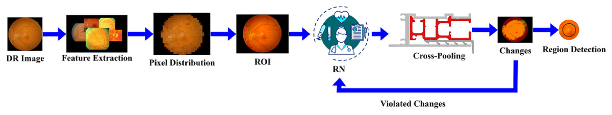
Figure 1: Functional architecture of the proposed GRIFD method.
Figure 1 illustrates the sequential operations in the GRIFD framework, including preprocessing of fundus images, feature extraction, pixel distribution analysis, ROI detection, recurrent learning, cross-pooling, and precision-driven region dissection.
RNN-based feature modeling
In the proposed work, a RNN is used as the core learning architecture to model temporal dependencies and spatial variations in DR lesions. The purpose of integrating the RNN is to iteratively process extracted feature sequences from fundus images and analyse changes in pixel intensity distribution across different ROI. The RNN’s memory state enables the system to retain contextual information from previously seen features, which is crucial for identifying subtle lesion progression or spatial inconsistencies that are not visible in isolated patches.
From the ROI examination, the maximum differences between features with higher variation are detected. Thus, the ROI-based examination is done for the maximum differences analysis. Hereafter, the following section focuses on the recurrent neural network where cross-pooling is observed to validate the variation process and improve the precision. The ROI is detected using maximum differentiated features in the sequential pixel distribution along the input image. The features with high variations within the identified ROI are dissected to determine the maximum changes. The following equation analyses the assessment layer used to store the previous data of the DR image.
(1) The assessment layer is processed to grasp the previous step of computation and produce the result. The assessment layer is responsible for performing the pixel identification from ROI and pursues the feature extraction process. This illustrates the feature extraction method determines the detection phase and it is pursuing the pixel distribution. The pixel distribution is done for variation identification and it is symbolized as . Based on this assessment, layer RNN grasps the previous step from number of layers and examines the cross-pooling method, which is described as . Post to this method, the memory state is used to reduce the complexity of DR image detection from the pixel distribution, and it is equated in the below derivative.
(2) The memory state is , the variation changes are observed and it is represented as , this step uses the assessment layer under RNN and stores the information regarding DR. Based on the DR information the severity is analyzed reliably, by computing the variation process. The recurrent neural network model for variation detection is portrayed in Fig. 2.
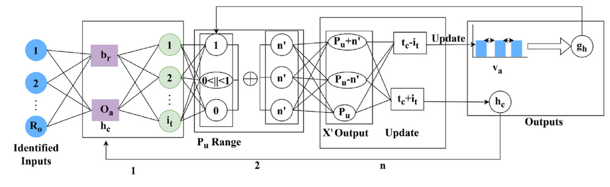
Figure 2: Recurrent neural network (RNN) model for DR feature variation detection.
Figure 3 shows how sequential features are passed through the RNN, how memory states preserve prior variation trends, and how cross-pooling detects dissimilarities between consecutive layers for accurate DR classification.
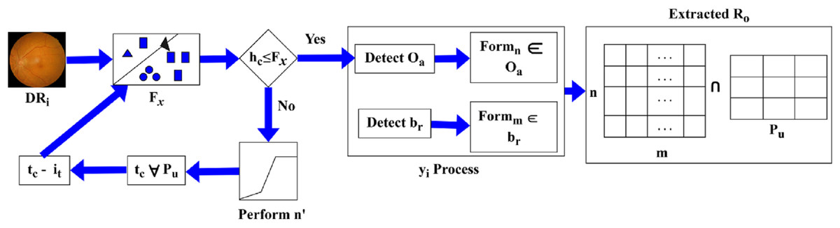
Figure 3: selection process for region dissection based on pixel distribution.
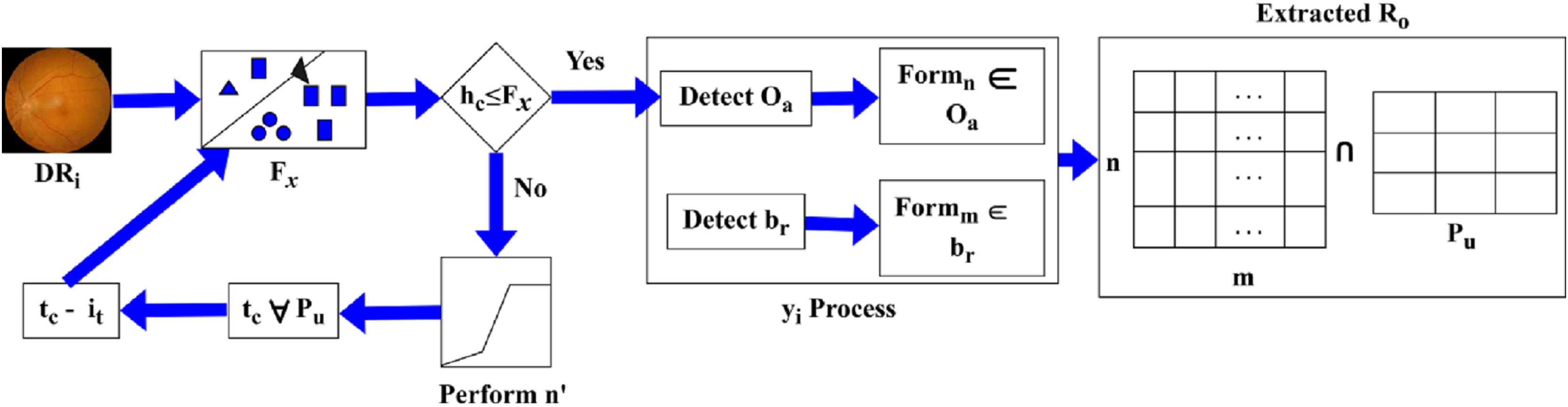
The RNN process mode for detection is illustrated in Fig. 2 for layers. The detected are the inputs for extracting using and . Using these variants of , the range as 0 or 1 or is defined. The range of is normalized to identify if is same output . If the parameters are not the same, then is the identified factor for layer outputs. However, this variation is less concerned with maximum/minimum changes. The consecutive number of and changes (differences) are used to define provided the recurrency is maintained. The mediate impacted by the in any output is assessed for such that is first performed. Irrespective of the to changes, the is the least possible changes identified. If this change is detected then the changes are exactly detected. This variation is examined by using the cross-pooling method and defines the memory state that computes the storage of the previous set of information as the assessment layer does. Post to this method the cross-pooling is done to check whether the variation decreases or not and it is evaluated below.
(3)
The cross-pooling is performed to analyse the variation and whether it decreases. The minimum range is , where it validates the DR image and efficiently examines the cross-pooling. Thus, the cross-pooling is used in the memory state and acquires the assessment layer. The variation decreases and consistency is maintained, and these changes are used to observe the higher and lower range of variation detection. This format defines the changes, and from this violation, changes are observed in the following equation.
(4)
The determination is processed for the violation changes that occur due to the variation check and measures the maximum and minimum format. The maximum is represented as , this stage uses the memory state for the identification of diseases and on which layer it relies. This determination is labelled as , where it computes the maximum and minimum ranges and the detection phase. The pixel distribution is followed up to find the violation changes that have minimum changes in this step, training is given and it is equated as follows.
(5)
The training is followed up in the above equation, which utilises the determination phase for analysing maximum and minimum values. This relies on the cross-pooling method and finds the variation detection and from this violation, changes are detected. If the violation changes are recognised, then the training is given and it is labelled as .
The selection of a RNN to be employed in the GRIFD framework is intentional and driven by its strength in modelling sequential dependencies in pixel-level feature changes between ROI blocks. In contrast to CNNs, which focus only on local spatial patterns, and Transformer models, which utilise global self-attention but are computationally expensive, the RNN efficiently models the evolution of features in spatially contiguous areas with minimal overhead. This works well in fundus images where lesions frequently appear as gradual, sequential changes and are less likely to appear as sudden changes. The memory state of the RNN allows the model to follow these fine changes across time and support the identification of accurate lesion boundaries while inhibiting inconsistent or false positive areas. Such sequential modelling, when added with our cross-pooling mechanism, is the strongest point of GRIFD in supporting higher precision and specificity along with minimal detection delay.
Proposed GRIFD framework
In the envisioned GRIFD model, the RNN module utilises a memory cell and a hidden state to track sequential shifts in feature activations between consecutive ROI blocks. This is borrowed from the temporal modelling properties of LSTM-based networks, commonly used in longitudinal medical image analysis. The cross-pooling violation pertains to situations where neighbouring regions produce contradictory pooled features, which are probably due to image noise or intra-anatomical structural overlap. To counter this, our cross-pooling procedure corrects inter-region continuity in accordance with ideas utilized in spatial feature calibration observed in attention-guided filtering approaches.
The feature extraction is done from the input DR image, and the features associated with the three stages are identified: mild, regular, and high. This examination step illustrates the variation process that is checked periodically under ROI. This extraction enables the accurate detection of DR, which is crucial for defining the recurrent neural network. This network represents the region in n x m matrices and finds its features. Here, the characteristics of the image are analysed, and the changes are exhibited under the variation process. This step defines the pixel distribution from the ROI and estimates the higher-level feature extraction process. The desired features are extracted reliably, and training is provided if any violations occur. Due to these violations, the constant range is not maintained under RNN. From this part of the study, the precision degrades, necessitating improvement in this examination step. The initial step is to validate the DR image using a normalisation approach, which is described below.
(6)
(7)
The validation is carried out in the above equation and it is represented as , the DR input image is symbolised as DR, and the feature extraction is denoted as , the brightness and contrast are termed as and . The periodic monitoring is represented as , is the time taken to perform the particular processing step. The evaluation occurs for the different feature extraction processes from the input DR image. Here, periodic monitoring is observed better, and the extraction is pursued reliably. Both the brightness and contrast are considered, and better analysis is performed for image retrieval from the database and detecting whether the diseases are standard, higher, or lower. Executing this step determines the period that considers the image’s brightness and contrast and performs better detection to improve the precision level, which is the scope of this work. The progression is executed reliably and illustrates the pixel-distribution stage.
Pixel distribution assessment
Before training the GRIFD model, two types of inputs were extracted from the fundus images: Feature-Based Inputs, these include textural and intensity-based descriptors such as mean intensity, local binary patterns (LBP), and histogram-based contrast variations computed within each ROI block. Each image was partitioned into non-overlapping n n blocks, from which first-order statistics and Gabor-filtered responses were collected as features. Edge-based inputs, for edge-oriented analysis, the same ROI blocks were passed through gradient-based filters (e.g., Sobel and Laplacian) to extract contour and vessel boundary features. Edge maps were then analysed for abrupt variation transitions using variance and entropy calculations across neighbouring pixel clusters. These extracted feature vectors were then standardised and normalised before being used as input to the recurrent neural network. The varying conditions (i.e., different lighting, contrast, lesion presence, and vessel occlusion) were simulated across images to evaluate the model’s robustness under multiple feature and edge conditions.
The pixel distribution assessment is performed using the extracted features; the initial stage is to validate the DR image using normalization. This normalization is carried out based on the pixel-distribution process, which defines the validation method. The validation is executed for the DR image extraction from the database and performs the normalisation that includes the brightness and contrast. Based on these two parameters, the feature of the DR is extracted and observes the better detection of variation. Here, the variation check is executed to examine the reliable processing step and verify the normalisation condition. This normalization is used to illustrate whether the image has higher brightness or contrast, and in other cases, lower brightness or contrast. On processing this evaluation, the validation runs through reliable feature extraction promptly. From this computation step, the analysis is conducted to detect DR within the specified severity range, and it identifies the specific characteristic, as formulated below.
(8)
(9)
The analysis is conducted for the specific characteristic used to detect DR images. The characteristic is represented as , is symbolised as pixel-distribution, the detection is . This is executed in the desired manner and that illustrates the periodic observation takes place on time. The evaluation step is executed for the varying DR image and is associated with the characteristic used for the analysis phase. This analysis, denoted as , is performed under different input image sets and examines pixel-based acquisition. This defines a more efficient processing step for the DR image and facilitates the variation check. The variation check is followed up for the DR and analysis of the characteristic, which refers to the light condition during image capture. Based on this capturing process, the study shows a slight variation in the input image. To improve the detection phase, the feature used to examine the characteristic-based input image is evaluated. This shows the image characteristic in the required manner for time-based computation.
Periodic observation is conducted to identify characteristic image features and accurately validate the pixel distribution. This evaluation is undertaken to facilitate the desired computation related to the timely observation of characteristics and provides the necessary steps accordingly. In this execution step, the analysis for the specific characteristic leads to detecting pixels on n × m matrices and gives the necessary step. This processing step is used to identify the DR image along with the features and characteristics and provides the appropriate detection phase. This includes the appropriate processing that estimates the memory state, which involves mapping the DR image’s previous data to the current data and is executed under the RNN. The computation performs feature extraction to provide necessary detection for characteristics and gives the parameters. This processing step is carried out based on the characteristics and features of the DR image. Following this observation process, feature extraction is performed using the equation below.
(10)
(11)
The feature extraction is executed in the above equation, which represents the DR image and is associated with a characteristic of the image. The evaluation takes place for the normalisation of DR, as discussed in equation, where the ROI is symbolised as . The normalisation is described as , the processing step is used to determine a better detection of pixel distribution for the improvement of precision. The precision level is maintained reliably, and it estimates the image characteristics process. The progression is used to define the image characteristic and find the validation and normalization of the input image. This input image is used to extract the necessary features and perform the detection phase. The detection plays a vital role in the validation process, exhibits the image’s feature and computes the variation. The pixel distribution is performed using DR detection and displays the ROI resulting from the pixel distribution. The selection process is defined using Fig. 3.
The Fig. 3 depicts how the proposed method selects ROI blocks by intersecting pixel-distributed features and evaluating them against feature variation thresholds to determine eligible dissection zones.
The is identified as an intersection between and extracted from . Depending on the identified, if then and for and are used to define the new region of . If the range exceeds the actual then is pursued as and for all . This process is computed towards and classification for differentiation such that is the sub-category of normalization performed from whereas, . Based on this difference between and , the is extracted. Hence, the process constitutes both and (Fig. 3). The extraction is done for the varying DR that is executed in the required manner and illustrates the matrices. In this methodology, validation is exhibited for the DR normalization process and evaluates the precision rate. By examining the severity range, the diseases are detected with the use of features and characteristics and pursue the extraction of necessary features. Only the necessary features are extracted within the required period, and a more thorough analysis of the memory state enables the periodic checking of variations that occur under ROI. Hereafter, the feature extraction is an important step that calculates the ROI using the DR image as input and exhibits validation. Validation and normalisation are used for the feature extraction, which includes the brightness and contrast. Based on this, the ROI is calculated using the pixel distribution method. From this approach, the necessary features are extracted from the DR, and a post-processing step is applied to the pixel distribution based on the extracted features, as formulated below.
(12)
The pixel distribution is done from the feature extraction process and that defines the better recognition of brightness and contrast. To identify the necessary features the pixel states the collection of blocks that appear on the DR image. From the feature, the segmentation is done as a pixel distribution that includes the block size. Here, the n × m is used to define the feature extraction process and periodically pursues the checking process. The n × m matrices are used under pixel distribution and they provide the appropriate detection of DR image. This processing step is used to define the matrix format in which the feature extraction is performed. The matrices used in this work are used to matrix the feature extraction process. The pixel distribution is carried out in the desired format, which exhibits the feature for the change area derived from the pixel-based distribution obtained through detection in the region. The ROI is used to determine this pixel distribution and provides the necessary steps accordingly. The brightness and contrast are used to evaluate the differences among the features.
The feature extraction is evaluated for the pixel distribution process and that defines the validation process for matrices. The ROI is calculated for the varying analyses and findings related to the severity of diseases at different stages. The normalization is followed up for the specific characteristic and estimates the desired processing. The progression runs through the analysis of the maximum difference between the features and with a higher variation rate. This variation rate differs based on the pixel-distribution technique, which exhibits the necessary feature extraction. The essential features extracted along with these characteristics are used to examine the periodic validation of DR and find the treatment. The treatment is carried out for the DR patient by identifying the region of interest, which is performed under pixel distribution. Hereafter, the examination is done for the ROI where the maximum difference between the features with higher variation is computed and expressed in the equation below.
(13)
The examination is done for the ROI features and it is described as X′, this includes pixel distribution and feature extraction. The processing step includes the n × m matrices that pursue the DR image and analysis is carried out. The analysis is followed up for the feature extraction and pixel distribution process, and defines a better recognition of DR from the input image. The examination is done for the ROI image that exhibits the detection phase and it is associated with the pixel distribution. From this, both the necessary features and pixel distribution are followed up on periodically to detect the DR.
Cross-pooling mechanism
From this estimation, variation detection is followed up as the iteration from RNN for change detection. The variations are the training inputs used for the detection of lower variation occurrences. Hereafter, the variation detection is examined in the following equations.
(14)
The variation change occurrences are analysed in the above equation, which exhibits the training phase for the minimum variation. These changes are done from the violation step, and it is labelled as , and evaluates the recognition of variation from high to low. If it occurs, then the change detection is carried out for the variation process, where the classification is processed, and it is represented in the equation below as follows.
(15)
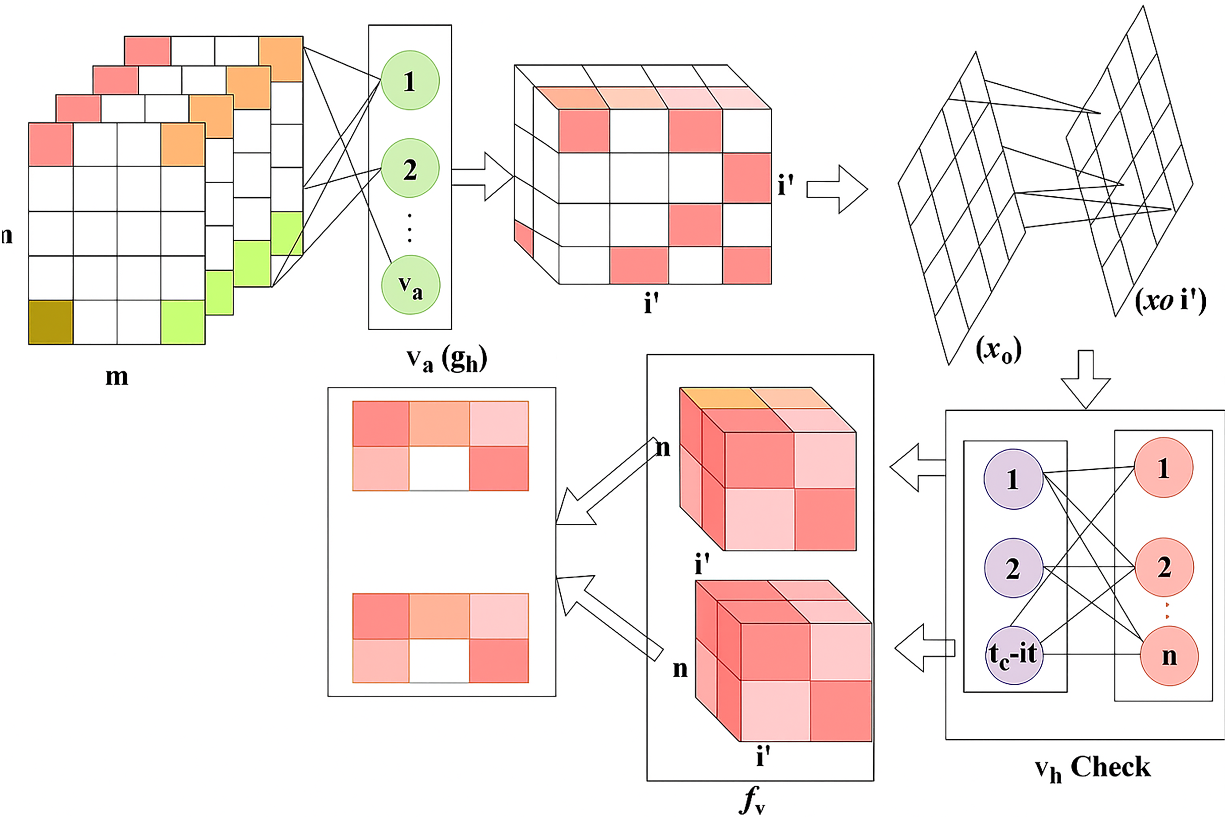
The change detection is performed and finds the ranges from high to low variant, from this case, the pixel distribution and feature extraction verifies the change detection occurrences reliably. The classification , is used to differentiate the maximum and minimum variation from the cross-pooling process among the layer’s representation. The cross-pooling process variation detection is portrayed in Fig. 4.
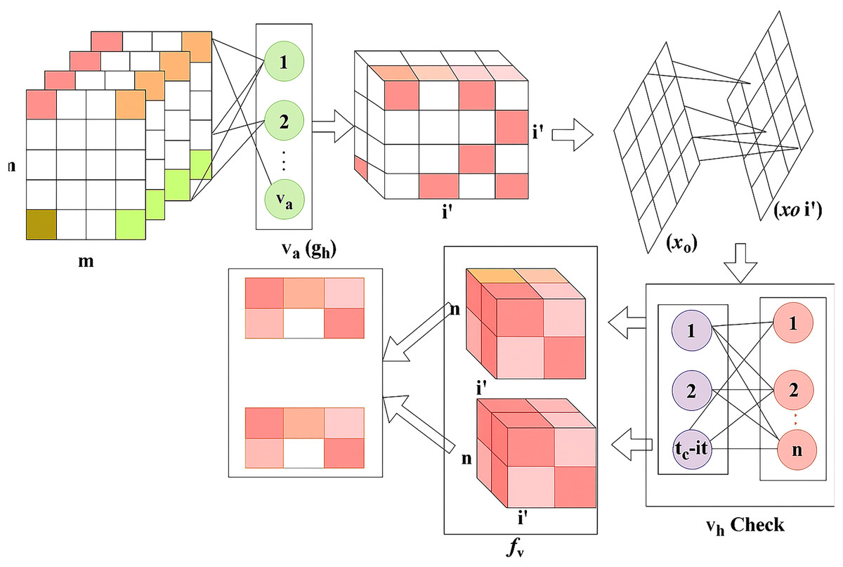
Figure 4: Cross-pooling estimation flow for variation detection.
Figure 4 presents the evaluation of variation levels (high or low) across RNN layers through cross-pooling, enabling the network to classify regions with precise control over changes and dissection logic.
The cross-pooling for detection relies on observed in and . Based on the input classification for and differentiations, the check is performed. From this computation, and for any range of . Considering this validation, the to is clubbed from the last known and detected. If the is less than the previous instance, then is the maximum change identified from . In case of a new detected from any , the is estimated from provided is the recent (updated) change. Therefore, the change is suppressed by supplementing (or) from the detected. Therefore, classifies and check as in Fig. 4. Thus, the change detection is executed for the classification model, and from this region, dissection is done from the change analyzed as maximum to minimum and it is identified below.
(16)
The identification is observed for the analysis of the maximum to minimum range of variation process and that illustrates the validation method for the feature extraction. The identification is termed as , which detects the phase for DR images and determines the cross-pooling techniques. The detection is carried out for the region dissected from the occurrences of the change in the variation process. The precision level improves, as shown below.
(17)
The precision level improves by decreasing the error rate, which is achieved through this reduction, as discussed in Eq. (2). The precision is , which defines the validation process for the cross-pooling method and provides the change occurrences from maximum to minimum variation; thus, region dissection is done using RNN. Therefore, the scope of this article is satisfied by using RNN for region dissection.
Results and discussion
Hyperparameter analysis
In the hyperparameter analysis, the variables related to dissection accuracy are identified and their impact on performance is studied. In this manner, the confusion matrix for and is represented in Fig. 5.
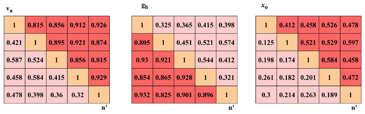
Figure 5: Confusion matrix visualization for accuracy, precision, and specificity metrics.
The confusion matrix shows the classification performance across different classes of DR severity, highlighting true positives, false positives, and false negatives obtained from the GRIFD.
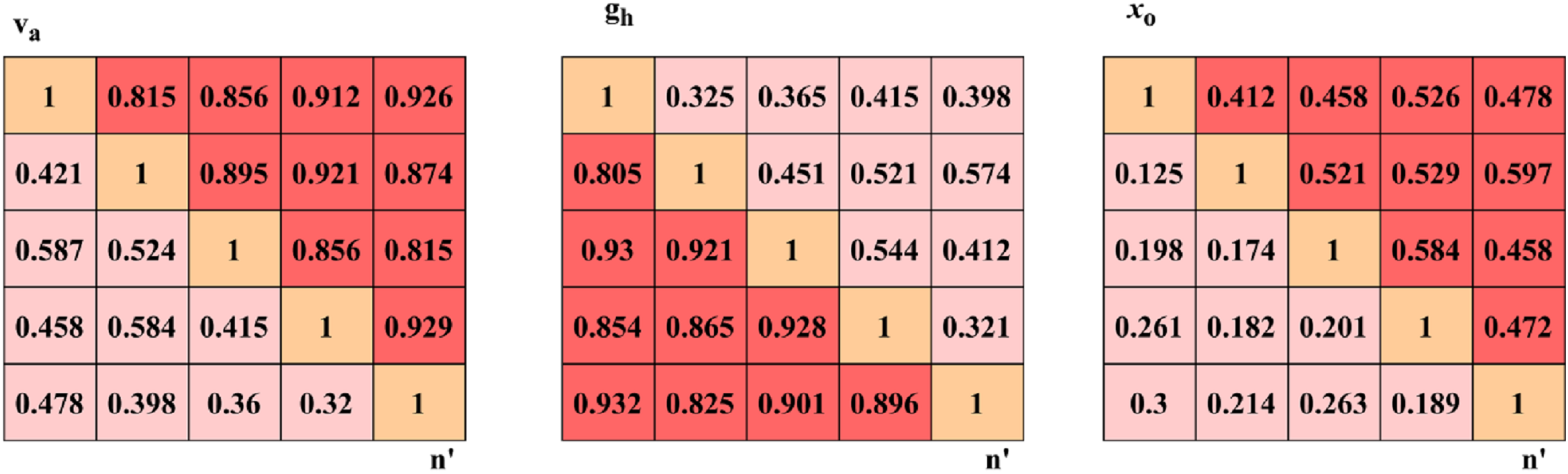
The and changes are abrupt by identifying from different . The for to is performed to verify if for any range of . The categorization of and are performed under the above three variants of such that delivers errorless . The recurrent processes of and is required to decide . Hence, the for the varying sizes is optimal to reduce the . The identifies the from the consecutive set of and mapping to ensure fewer errors are identified. Thus, the new relies on the target of for reducing the that maximizes the dissection of and . Therefore, the outputs are sufficient to maximize the dissection accuracy (Fig. 5). The ROC for and is analysedmaximise as presented in Fig. 6.
Figure 6: ROC curve for true positive rate (TPR) vs. false positive rate (FPR).
(A) ROC curve for dataset Va showing TPR vs. FPR for computed and actual results. (B) ROC Curve for dataset 9b showing TPR vs. png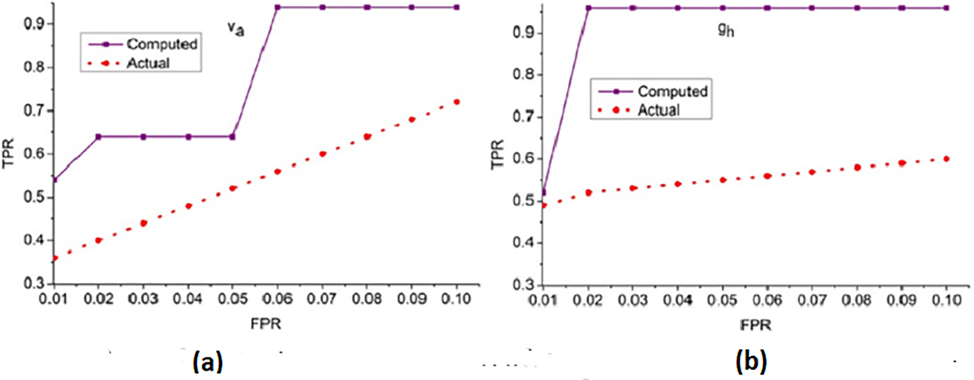
The receiver operating characteristic curve illustrates the TPR against the FPR for different thresholds, demonstrating the classification capability and sensitivity of the proposed method.
The true positive rate (TPR) for the false positive rate (FPR) for and is analyzed in Fig. 6. The is the objective for accuracy improvement regardless of and . The recurrent learning process identifies the exact and variants from the actual . In the condition validation of , the with maximum is suppressed. This reduces the chance of FPR for by performing and such that existing is sufficient for increasing accuracy. The and regulates the by identifying from to ensure reduces the error and thereby the training retains the maximum for accuracy improvement. In the final hyperparameter analysis, the error is considered and presented in Fig. 7.
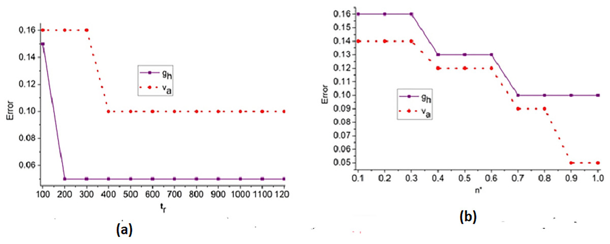
Figure 7: (A) Error trend across iterations for feature-based analysis. (B) Error trend across iterations for edge-based analysis.
Figure 7 illustrates the convergence pattern of the error metric over multiple training iterations, indicating the robustness of the model for different feature and edge types.
The error analysis for the iterations and is presented in the above Fig. 7. The is the optimal case for reducing and under different . Based on the to outputs the priority is defined; this instance identifies the to or variant by identify changes. Depending on the and differences in from any layers, the improvement is pursued. Therefore, the is revisited using that validates to reduce . If this is achieved then X′ for all ad are equated for similar congruency and specificity. Therefore, the least serves as the point for any range of FPR observed. The region combining and is segregated from to to ensure fewer errors under and .
Experimental setup and results
The proposed method is evaluated using MATLAB codes executed in a standalone computer with 4 GB-2slots random memory and a 2.1 GHz Intel processor with a storage of 128 GB.
Before training the GRIFD model, two types of inputs were extracted from the fundus images: Feature-based inputs include textural and intensity-based descriptors, such as mean intensity, local binary patterns (LBP), and histogram-based contrast variations computed within each ROI block. Each image was partitioned into non-overlapping n n blocks, from which first-order statistics and Gabor-filtered responses were collected as features. For edge-oriented analysis, the same ROI blocks were passed through gradient-based filters (e.g., Sobel and Laplacian) to extract contour and vessel boundary features. Edge maps were then analysed for abrupt variation transitions using variance and entropy calculations across neighbouring pixel clusters. These extracted feature vectors were then standardised and normalised before being used as input to the recurrent neural network. The varying conditions (i.e., different lighting, contrast, lesion presence, and vessel occlusion) were simulated across images to evaluate the model’s robustness under multiple feature and edge conditions.
Dataset
The testing fundus image inputs are fetched from Akram et al. (2020) which contains 100+ fundus images of patients between 25 and 80 years of age. The digital image resolution is pixels of which 76 are infected with DR. The learning rate is set between 0.8 and 1.0 for 1,200 iterations under three epochs. The training images are 100 and the testing image count is 76 for which the epochs are repeated for maximum precision. This dataset contains retinal blood vessel networks, segmented artery and vein networks, and a testing image count of 76. It is used to calculate the arteriovenous ratio (AVR), annotate the optic nerve head (ONH), and identify various retinal abnormalities, such as hard exudates (HE) and cotton wool spots. we employed a grid search strategy combined with 5-fold cross-validation on the Mendeley dataset to identify optimal values for learning rate, batch size, number of epochs, and dropout rate. Performance was evaluated based on validation accuracy and mean error across folds.
These images are organised into distinct categories based on retinal conditions, including DR, hypertensive retinopathy, papilledema, and normal. While the dataset provides folder-level grouping for these four diagnostic classes, it does not include explicit annotations for the different stages of DR (such as mild, moderate, or severe). Therefore, any further categorisation by DR severity must be performed manually based on visual inspection of retinal lesions such as microaneurysms, haemorrhages, and exudates, or through clinical labelling where available. This dataset serves as a valuable resource for evaluating both segmentation and classification algorithms in the context of retinal disease detection. Figure 8 presents the identified ROIs from test images using the GRIFD model, with a focus on severity-based visual segmentation across different DR stages.
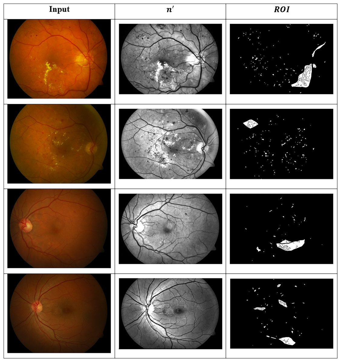
Figure 8: ROI detection outputs for sample fundus images.
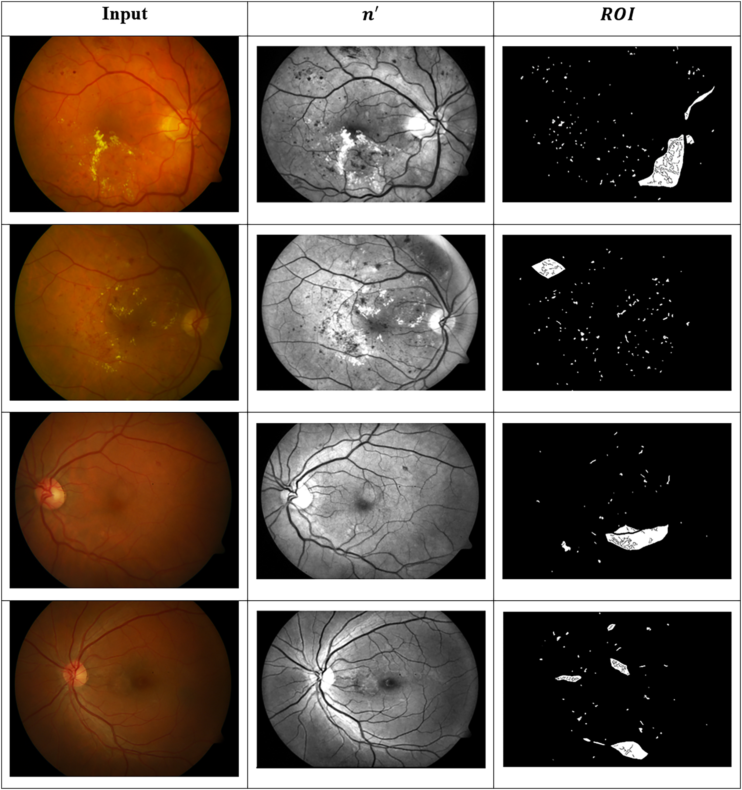
Figure 9 presents visual or matrix-based results of lesion region segmentation and dissection after applying feature variation analysis and RNN-based validation.
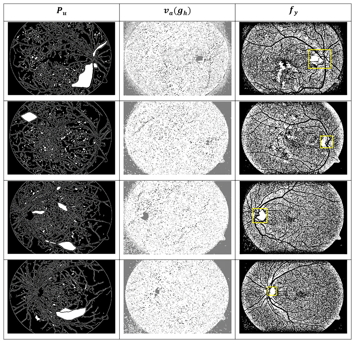
Figure 9: Dissected lesion region outputs from GRIFD method.
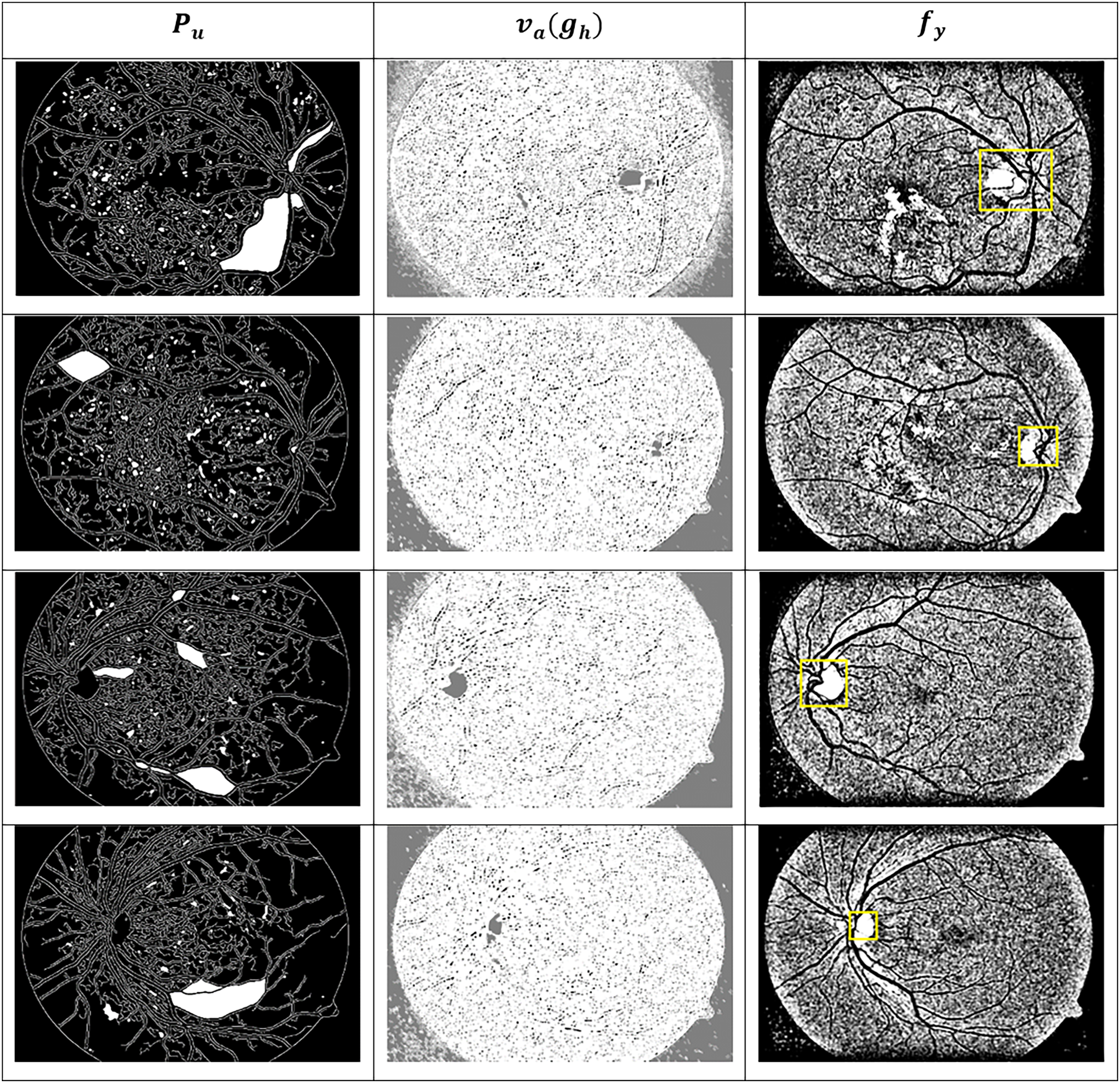
The dataset for the current study comprises more than 100 colour fundus images from the Mendeley Data repository (Akram et al., 2020), which contain various retinal conditions, including diabetic retinopathy. A total of 100 images were manually examined and selected for training and testing, 24 normal, 28 mild DR and 48 severe DR—a balance across the spectrum of severity. All images were rescaled to 512 512 and underwent preprocessing operations, including grayscale conversion, contrast normalisation, histogram equalisation, and median filtering for denoising. ROI-based cropping was used to focus on central retinal areas. Annotation validity was ensured by referencing the metadata and folder structure in the dataset. In instances where severity labels were not available, clinical features such as microaneurysms and haemorrhages were visually examined and labelled by expert annotators to preserve the ground truth.
A dropout layer with a rate of 0.3 was applied after the RNN and fully connected layers to reduce co-adaptation of neurons and minimise overfitting. Additionally, L2 regularization with a coefficient of 1e−4 was applied to the weights during training. For the Mendeley dataset, we applied basic augmentation techniques including horizontal flipping, rotation ( 15 degrees), brightness scaling ( 10%), and minor Gaussian blurring to synthetically expand the training set and introduce variability in lesion appearance. These augmentations were applied in real time during each training epoch.
Comparative analysis
The comparative analysis is presented using the metrics: accuracy, precision, specificity, mean error, and segment detection time. These metrics are analysed under the varying features and edges, and therefore, they vary in number (1–12) and (1–9), respectively. To verify the proposed method’s efficiency, the method is compared with the existing RTNet (Huang et al., 2022), MCNN-UNet (Skouta et al., 2022), and DRFEC (Das, Biswas & Bandyopadhyay, 2023) methods.
To assess the performance of the proposed GRIFD method, the following standard metrics are used: Accuracy (Acc) is the proportion of correctly predicted observations (both DR and non-DR) out of the total observations.
(18)
Precision (Prec) is the ratio of true positive predictions to the total predicted positive cases. It reflects the model’s ability to correctly identify DR.
(19)
Specificity (Spec) is the ability of the model to correctly identify non-DR cases (true negatives).
(20)
Mean error (ME), is the average absolute error between predicted and actual region boundaries or lesion locations. This is computed across all tested images.
(21) where is the predicted value and is the actual ground truth. Detection delay ( ) is the average computational time (in seconds) taken by the model to detect and localise the DR region per image.
To conduct fair and consistent comparison all three methods (Huang et al., 2022; Skouta et al., 2022 and Das, Biswas & Bandyopadhyay, 2023) were re-implemented and trained on the same fundus image dataset used in the proposed GRIDF method. RTNet is a transformer-based architecture that applies self-attention mechanisms to establish relational dependencies between lesions and their corresponding vessel features in fundus images. It combines the accuracy of a relation encoder-decoder framework to perform multi-lesion segmentation. The MCNN-UNet method combines a multi-channel CNN feature extractor with a U-Net-inspired decoder for the task of hemorrhagic regions segmentation, preserving the channel-wise feature hierarchies. The DRFEC method consists of a convolutional feature extraction process and a fully connected classification process to identify and compare severity of DR-related abnormalities due to their structure and texture in associated vessels. The number of images, training methods and parameters, and the dimensions of what the network sees remained consistent and each method was trained from scratch. For both training (100 images) and testing (76 images), the same image set from the Mendeley Data (Akram et al., 2020) repository was used. These scenarios enable the evaluation of the most expansive metrics, including accuracy, precision, specificity, mean error, and detection delay,the through both training and testing across the three methods.
Accuracy
Figure 10 compares the accuracy metric for the proposed and existing methods across multiple feature and edge variations, showing superior performance of GRIFD.
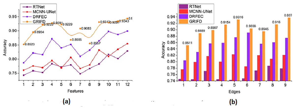
Figure 10: Accuracy comparison among GRIFD, RTNet, MCNN-UNet, and DRFEC.
(A) Accuracy of proposed and existing methods for various feature variations. (B) Accuracy comparison of different edge variation.
The accuracy rate for the proposed work is high (Fig. 10) for varying features and edges and that purses the feature extraction process and estimates the pixel distribution. The input DR image is acquired, and the feature extraction process is performed here, resulting in n × m matrices that are accurately followed up. This illustrates the better recognition of ROI from the two matrices and provides the distribution factor. The validation is performed for image normalisation, which in turn supports the severity analysis for disease detection. The varying stages are used to explore the ROI and provide an estimation process by using an RNN. The necessary feature is extracted by detecting changes in occurrence. Here, the training is given to the RNN and that is associated with the cross-pooling process. The accuracy rate for the proposed work is used to determine the pixel distribution, based on the extraction. Achieving accuracy plays a significant role in this proposed work and employs the normalization of the DR image. This is associated with the severity caused by the diseases and address and it is formulated as .
Precision
Figure 11 shows how GRIFD outperforms other methods in terms of precision by effectively identifying regions with maximum variation across fundus images.
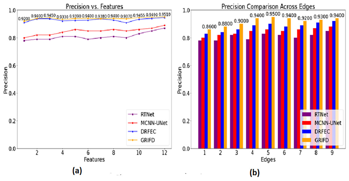
Figure 11: Precision comparison for DR region identification.
(A) Precision for various feature variations in DR region identification. (B) Precision for different edge variations shown.
The precision in this work is improved (Fig. 11) by identifying the maximum difference between the features that show the higher variation changes. This is observed in two metrics such as features and edges of the DR image and that is associated with the pixel distribution. Based on this proposal the validation is followed by the training phase that uses the memory state under RNN. This methodology illustrates the feature extraction process and defines the specific characteristics of the image. Both the image’s feature and unique characteristics are considered to give the necessary result. In this manner, it determines the accuracy of the DR image that envelopes the examination step and provides the n × m matrices. This processing step defines the normalization of the image by validation process and examines the violation changes. The violation changes occur due to the feature extraction process and accurately define the precision level and it is equated as , here it shows a higher precision rate.
Specificity
The Fig. 12 compares the specificity scores, reflecting how accurately each method avoids false positives while detecting DR-affected regions.
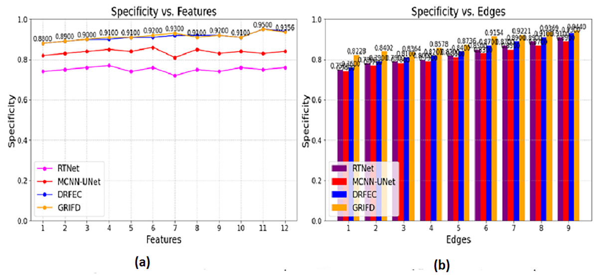
Figure 12: Specificity values for feature and edge-based dissection.
(A) Specificity for feature-based DR region detection. (B) Specificity for edge-based detection showing fewer false positive.
The specificity is computed for the pixel distribution and uses , for the DR images. This estimates the necessary feature extraction process that illustrates the variation change occurrences. The variation changes define the reliable specificity among the DR images and detect the diseases. Periodic monitoring is observed in this category, which determines the precision level of accuracy. This methodology is developed to explore the variation and gives the feature-based processing for the features. These features are associated with the variation changes and provide the training phase. The training is given based on this violation changes are analyzed based on the pixel-based image. From this processing step, the extraction is monitored for n × m matrices, and the resultant is generated accurately. This section focuses on two varying metrics such as features and edges; based on these the specificity shows a higher value range. To explore the differences between the features that rely on higher variation and determine the specificity it is represented as (Fig. 12).
Mean error
Figure 13 shows the mean error of region detection for all compared methods, indicating significant improvements with the proposed cross-pooling-based dissection.

Figure 13: Mean error reduction achieved by the GRIFD method.
(A) Mean error for feature-based region detection. (B) Mean error for edge-based detection, showing reduced errors.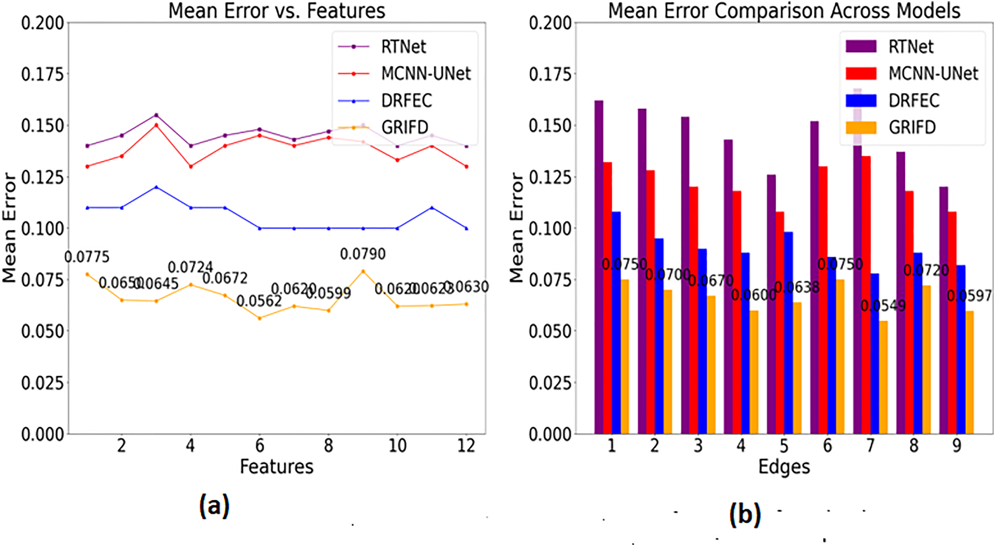
In Fig. 13, the mean error is found to be less based on the specific characteristics and features. Based on this approach, the training phase is carried out in the desired manner, resulting in matrix-oriented processing. This matrix shows the pixel distribution among the input image and that is forwarded to the ROI. The ROI image is extracted from the pixel distribution, which relates to the cross-pooling mechanism. The pooling is used to check for the variation, ranging from higher to lower. If it is lower, the necessary training is given based on the feature distribution. The distribution is followed up for the violation changes and detects for the region distributed process. The scope of this work is to attain the region disserted and observe the variation process among the features. The cross-pooling is carried out in the desired way that explores the addressing of mean error in this work and reduces it is equated in Eq. (17) where the precision and error rate are equated and it is symbolised as .
Detection delay
Figure 14 highlights the efficiency of GRIFD in reducing detection time, making it more suitable for real-time or rapid screening scenarios.
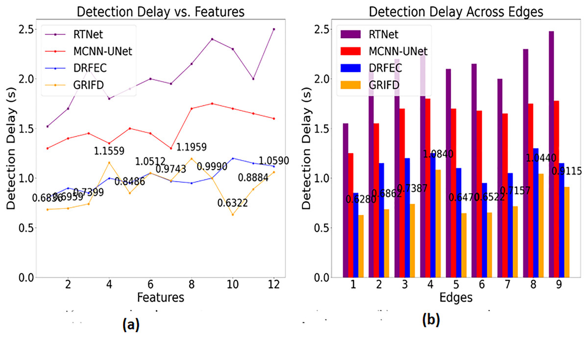
Figure 14: Detection delay comparison among DR detection methods.
(A) Detection time for feature-based analysis (B) detection time for edge-based analysis, showing faster processing.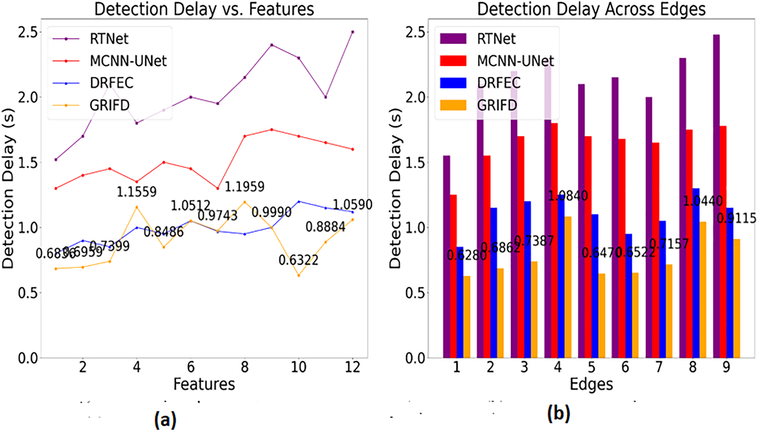
The detection delay is reduced in this proposed work which shows lesser value compared to the previous methods (Fig. 14). This progresses under two metrics such as features and edges, and gives the ROI-based image processing. The image processing runs through the desired computation and that relates with the region dissected. From this the precision level is improved and the error rate is reduced by considering this process so that the delay is addressed and shows a better DR image. The DR image is used to envelop the cross-pooling mechanism and relates with the pixel distribution among n × m matrices. Both the matrices are associated with changes occurrences due to the variation that is performed under variation changes. Thus, it explores the violation changes given to the training section and examines the better pixel distribution phase. This step is processed among the specific characteristics to explore the variation changes and reduce the delay factor. This detection is associated with the ROI region extraction and delay is addressed and it is formulated as .
Comparison with literature survey
A few recent works suggested varied methods to enhance diabetic retinopathy (DR) detection with their respective accuracy rates and architectural designs. Huang et al. (2022) presented RTNet as a model utilising transformers, along with relational self-attention, for multi-lesion segmentation, achieving an accuracy of 92.2%. Although RTNet excels at structurally modelling the dependencies of features across spatial context spaces, the model does not support sequential dissection, thereby precluding the ability to extract the subtle progression of the lesion over time. Mishra, Pandey & Singh (2024) employed an ensemble deep neural network (DNN) framework, achieving 88% accuracy. Though ensemble methods often enhance robustness, their performance may degrade in the presence of noisy or overlapping features due to a lack of explicit region-level dissection.
Guo & Peng (2022) put forwarded the model of CARNet, where attentive refinement was used for DR segmentation with multi-lesion and attained good accuracy of 93%. However, the model of CARNet becoming space-attention-fusion-dependent and lacking temporal context verification sometimes causes inconsistency in the identification of lesion boundaries at different pixel intensities. Wong, Juwono & Apriono (2023) used a transfer learning approach with parameter optimization and ECOC ensemble classification, but reported only 82.1% accuracy. This lower performance may be attributed to domain mismatch and limited adaptability of pre-trained features to the diverse lesion types in fundus images. Singh & Dobhal (2024) reported 92.66% accuracy using a DL-based transfer learning model, demonstrating competitive results. However, the model’s dependence on static feature representations constrains its ability to model evolving lesion characteristics across image sequences. Table 1 provides a comparison of results with the literature survey.
| Reference | Method | Accuracy (%) |
|---|---|---|
| Huang et al. (2022) | RTNet | 92.2 |
| Mishra, Pandey & Singh (2024) | Ensemble DNN | 88.0 |
| Guo & Peng (2022) | CARNet | 93.0 |
| Wong, Juwono & Apriono (2023) | TL (Parameter Opt and ECOC) | 82.1 |
| Singh & Dobhal (2024) | DL-based TL | 92.6 |
| Singh, Gupta & Dung (2024) | Fine-tuned DL model | 74.5 |
| Naz et al. (2024) | Fuzzy Local K-means | 94.0 |
| Proposed method | GRIFD method | 94.35 |
Singh, Gupta & Dung (2024) presented a fine-tuned deep learning model, but achieved only 74.58% accuracy, indicating a lack of generalization capacity, possibly due to limited training diversity or insufficient feature dissection. Naz et al. (2024) presented an enhanced fuzzy local information k-means clustering approach, which provided the best accuracy of 94.00% compared to the methods discussed above. Though encouraging, the clustering-based scheme has limited contextual learning over depth and is prone to hyperparameter sensitivity when the distribution of the lesion is highly variable. With the above methods suggested by each author in the above table as comparison methods, the suggested GRIFD method had accuracy rates of 94.35% (features) and 93.72% (edges). This work rivals each of the above methods or outperforms them. The edge of GRIFD lies in its graded region-of-interest dissection, cross-pooling-based variation filtering and RNN-based sequential learning simultaneously allow the model to actively abolish false positives and stably retain lesion structures throughout the ROI. Unlike static methods based on attention alone or transfer learning alone, GRIFD formally verifies the pixel-level consistency and derives the high-variation regions by itself and hence ensures precise segmentation even under challenging image conditions.
Cross validation and comparison with additional dataset
To further test the generalizability of the suggested GRIFD approach, we experimented with the publicly accessible EyePACS dataset, a large set of diverse colour fundus images with diabetic retinopathy severity level annotations. We randomly selected 1,000 images (balanced by normal, mild, moderate, and severe diabetic retinopathy) from the EyePACS dataset for testing. These were preprocessed using the identical pipeline outlined above. The GRIFD model was also trained employing a 5-fold cross-validation approach to guarantee robustness. Results showed uniform performance across folds, with a mean accuracy of 93.85%, precision of 94.20%, and specificity of 92.78%, validating the method on a larger dataset with enhanced variability in image quality and lesion distribution, as shown in Table 2.
| Fold | Accuracy (%) | Precision (%) | Specificity (%) | Mean error | Detection delay (s) |
|---|---|---|---|---|---|
| Fold 1 | 93.70 | 94.10 | 92.60 | 0.058 | 1.02 |
| Fold 2 | 93.90 | 94.25 | 92.85 | 0.056 | 0.99 |
| Fold 3 | 93.80 | 94.30 | 92.70 | 0.055 | 1.01 |
| Fold 4 | 93.95 | 94.10 | 92.90 | 0.054 | 1.00 |
| Fold 5 | 93.95 | 94.25 | 92.80 | 0.053 | 0.98 |
| Average | 93.85 | 94.20 | 92.78 | 0.0552 | 1.00 |
To evaluate the generalizability and robustness of the presented GRIFD model, we conducted 5-fold cross-validation on the original Mendeley dataset as well as on the larger EyePACS dataset. As presented in Table 3, GRIFD performed uniformly well for all folds on the EyePACS dataset with an average accuracy of 93.85%, precision of 94.20%, and specificity of 92.78%. The detection delay remained constant at 1.00 s, proving the suitability of the method for real-world application. This performance ensures that the GRIFD algorithm maintains accuracy on a larger and more varied dataset, where differences in image quality, lesion size, and class distribution are greater.
| Fold | Accuracy (%) | Precision (%) | Specificity (%) | Mean error | Detection delay (s) |
|---|---|---|---|---|---|
| Fold 1 | 93.60 | 95.75 | 94.40 | 0.056 | 0.96 |
| Fold 2 | 94.20 | 96.15 | 94.80 | 0.054 | 0.95 |
| Fold 3 | 94.10 | 95.90 | 94.70 | 0.053 | 0.97 |
| Fold 4 | 94.50 | 96.20 | 95.10 | 0.055 | 0.96 |
| Fold 5 | 94.40 | 96.25 | 95.15 | 0.054 | 0.95 |
| Average | 94.16 | 96.05 | 94.83 | 0.0544 | 0.958 |
Table 3 shows the results of 5-fold cross-validation on the Mendeley dataset. GRIFD had excellent accuracy for all folds, having an average accuracy of 94.16%, precision of 96.05%, and specificity of 94.83%, and a smaller mean error of 0.0544. The mean detection delay was 0.958 s, which reflects the model’s low-latency nature. These findings confirm that GRIFD is not only accurate in its predictions but also consistent across diverse subsets of the same set.
A comparative overview in Table 4 identifies that GRIFD was slightly better on the Mendeley dataset (in single-run as well as cross-validation environments) than on EyePACS, as could be anticipated from the fact that Mendeley contains tidier, more uniformly preprocessed images. Yet the slight degression in EyePACS performance reaffirms the model’s ability to generalize, as it continues to post robust metrics without significant loss of performance. This shows that the suggested GRIFD architecture can transfer successfully to other datasets with maintaining both diagnostic accuracy and computational cost.
| Dataset | Validation type | Accuracy (%) | Precision (%) | Specificity (%) | Mean error | Detection delay (s) |
|---|---|---|---|---|---|---|
| Mendeley (Single Run) | Hold-out (76 test) | 94.35 | 96.05 | 94.91 | 0.0545 | 0.9625 |
| Mendeley (5-Fold CV) | Cross-Validation | 94.16 | 96.05 | 94.83 | 0.0544 | 0.958 |
| EyePACS (5-Fold CV) | Cross-Validation | 93.85 | 94.20 | 92.78 | 0.0552 | 1.00 |
Ablation study
An extensive ablation analysis was performed to analyse the effect of every main component in the GRIFD framework. The complete model achieved the highest performance overall, with 94.16% accuracy, 96.05% precision, and the most minor mean error and detection delay. The elimination of the cross-pooling layer resulted in a significant decline in specificity and precision, underscoring its crucial role in filtering out unreliable feature variations. Removing the RNN module impaired sequential learning, bringing accuracy down to 89.45%, replacing graded ROI dissection with uniform segmentation affected region localization and boosted the false positive rate. Last but not least, skipping preprocessing improvements yielded the worst accuracy (88.90%) and error rate due to unnormalized contrast and brightness levels in the input images. These findings indicate clearly that both modules are making significant contributions to the system overall, with cross-pooling and RNN taking centre stage in enhancing lesion boundary verification and classification resiliency. Table 5 shows an ablation study with the Mendeley dataset.
| Configuration | Accuracy (%) | Precision (%) | Specificity (%) | Mean error | Detection delay (s) |
|---|---|---|---|---|---|
| Full GRIFD model | 94.16 | 96.05 | 94.83 | 0.0544 | 0.958 |
| Without cross-pooling | 91.80 | 92.55 | 90.10 | 0.0685 | 1.12 |
| Without RNN (only CNN features) | 89.45 | 90.30 | 88.20 | 0.0721 | 1.25 |
| Without ROI-based graded dissection | 90.20 | 91.45 | 89.60 | 0.0653 | 1.18 |
| Without preprocessing enhancements | 88.90 | 89.10 | 87.10 | 0.0738 | 1.27 |
Statistical validation
To statistically validate the observed performance gains, we conducted a 5-fold paired t-test comparing the complete GRIFD model to its reduced variants. The t-test results showed that the whole model’s improvement in accuracy over the cross-pooling-removed version was statistically significant (p = 0.0032), as was its improvement in precision (p = 0.0047). Additionally, the 95% confidence intervals for GRIFD’s average accuracy and precision were [93.72%, 94.59%] and [95.75%, 96.35%], respectively, indicating high reliability and low variance in performance. These findings confirm that the enhancements introduced by GRIFD are not only consistent but also statistically meaningful.
Summary
The comparison of performances in Tables 6 and 7 emphasizes the better performance of the proposed GRIFD model compared to both existing methods (RTNet, MCNN-UNet, DRFEC) and conventional deep learning baselines (CNN, LSTM, CNN-LSTM, Transformer). On the feature level, GRIFD obtained the best accuracy (94.35%), precision (96.05%), and specificity (94.91%), while having the smallest mean error and detection delay. Equivalently, at the edge level, GRIFD also outperformed with 93.72% accuracy and 96.17% precision. Baseline models such as CNN and LSTM, on the other hand, demonstrated considerably poor specificity and detection times. These findings validate that GRIFD’s integration of cross-pooling, RNN sequencing, and ROI-based dissection greatly contributes to both consistency in segmentation and reliability in lesion classification across different areas in fundus images. Table 6 compares GRIFD with RTNet, MCNN-UNet, and DRFEC based on five evaluation metrics (accuracy, precision, specificity, mean error, and detection delay) using features as the basis for analysis.
| Model | Type | Accuracy | Precision | Specificity | Mean error | Detection delay (s) |
|---|---|---|---|---|---|---|
| RTNet | Published | 0.829 | 0.838 | 0.776 | 0.139 | 2.190 |
| MCNN-UNet | Published | 0.855 | 0.874 | 0.813 | 0.104 | 1.740 |
| DRFEC | Published | 0.899 | 0.926 | 0.891 | 0.089 | 1.330 |
| CNN (Simple-5 layer) | Baseline | 0.874 | 0.889 | 0.856 | 0.077 | 1.400 |
| LSTM (Single-layer) | Baseline | 0.892 | 0.898 | 0.873 | 0.071 | 1.300 |
| CNN-LSTM Hybrid | Baseline | 0.916 | 0.927 | 0.900 | 0.064 | 1.200 |
| Transformer (ViT-Base) | Baseline | 0.921 | 0.933 | 0.911 | 0.061 | 1.350 |
| GRIFD | Proposed method | 0.9435 | 0.9605 | 0.9491 | 0.0545 | 0.9625 |
| Model | Type | Accuracy | Precision | Specificity | Mean error | Detection delay (s) |
|---|---|---|---|---|---|---|
| RTNet | Published | 0.779 | 0.823 | 0.774 | 0.113 | 2.180 |
| MCNN-UNet | Published | 0.821 | 0.871 | 0.829 | 0.104 | 1.850 |
| DRFEC | Published | 0.874 | 0.912 | 0.902 | 0.082 | 1.325 |
| CNN (Simple-5 layer) | Baseline | 0.857 | 0.875 | 0.840 | 0.084 | 1.450 |
| LSTM (Single-layer) | Baseline | 0.873 | 0.882 | 0.855 | 0.078 | 1.320 |
| CNN-LSTM Hybrid | Baseline | 0.895 | 0.910 | 0.882 | 0.069 | 1.180 |
| Transformer (ViT-Base) | Baseline | 0.909 | 0.922 | 0.897 | 0.063 | 1.310 |
| GRIFD | Proposed method | 0.9372 | 0.9617 | 0.9448 | 0.0572 | 0.9198 |
The proposed GRIFD improves accuracy by 8.25%, precision by 8.12% and specificity by 12.24%. This method reduces mean error by 11.23% and detection delay by 9.04%. Table 7 provides a similar comparison as Table 6 but evaluates the metrics based on edge features, confirming GRIFD’s superiority in structural and boundary-based analysis.
The proposed GRIFD improves accuracy by 11.25%, precision by 9.3% and specificity by 10.98%. This method reduces mean error by 8.49% and detection delay by 9.69%. The observed improvements in precision and specificity can be directly attributed to GRIFD’s modular innovations. The graded ROI dissection improved lesion localization, while the cross-pooling module filtered spatial noise. Meanwhile, the RNN layer provided contextual continuity. These contributions collectively reduce misclassification and enhance decision reliability, as confirmed by the ablation results.
Limitation
Although GRIFD generally exhibits good performance, some instances of failure were observed. Misclassifications were primarily seen in low signal-to-noise ratio images, motion-blurred images, or in images where lesions become indistinguishable from the vascular tissue. Moreover, when trained on very imbalanced datasets like EyePACS, the model was found to have slightly lower sensitivity in minority classes. These mistakes imply that future research should incorporate sophisticated data balancing methods and adaptive attention components to enhance robustness. Another restriction exists in the sequential RNN inference, though optimised, which may be outperformed by parallelised attention-based options for increased speed and lesion boundary sensitivity.
Conclusion
This article proposed the graded region-of-interest feature dissection method to improve the precision of DR segmentation from fundus images. The accuracy is improved by reducing the feature variations from a range of randomly distributed pixels. The features are identified through continuous dissection of variation based on their range. This range is validated by identifying replicated features through edge classifications. The proposed method incorporates cross-pooling to identify and reduce high pixel variations. Therefore the recurrent analysis of the learning aids in determining the features that fail cross-pooling to reduce mean distribution errors due to false rates. Additionally, the low-variation violating features are filtered after the cross-pooling process to enhance precision. The violation involves feature dissection on continuous distribution sequences used to train the learning network based on specificity. Thus, the proposed method retained 8.12% of precision and 12.24% of specificity to reduce 11.23% of the mean error.
While GRIFD demonstrates high performance in terms of accuracy, precision, and detection speed, it is not without limitations. The model currently relies on fixed ROI dissection and lacks an adaptive attention mechanism, which may impact generalisation to fundus images with varying resolutions and qualities. Additionally, although RNNs effectively model sequential pixel transitions, they may introduce latency when scaled to high-resolution inputs. Future work will explore replacing RNNs with lightweight transformer-based modules to improve parallelism and scalability. Integrating self-supervised pretraining and domain adaptation strategies will also be considered to reduce dependency on labelled data. Finally, multi-centre validation on diverse clinical datasets will be performed to strengthen generalizability and clinical robustness.
The proposed method’s dissection property is limited to the classification performed after cross-pooling. This limitation will likely be saturated for precision estimation over homogeneous pixel distribution for even-sized fundus images. Therefore, the possibilities of classification are limited to the false rate computed. To address this problem, a cross-sectional dissection model with the same pooling is required in future work.
Supplemental Information
Implementation code.
The complete MATLAB source code for implementing the proposed GRIFD framework, including scripts and functions for training, evaluation, and result reproduction.
Implementation code.
Python script that implements a multi-objective genetic algorithm using DEAP, designed to optimize efficiency and fairness in an energy market scenario, with built-in visualization of results.