
MLPruner: pruning convolutional neural networks with automatic mask learning
- Published
- Accepted
- Received
- Academic Editor
- Stefano Cirillo
- Subject Areas
- Computer Vision, Data Mining and Machine Learning, Neural Networks
- Keywords
- Filter pruning, Mask learning, Straight-through estimator
- Copyright
- © 2025 Chen and Zhao
- Licence
- This is an open access article distributed under the terms of the Creative Commons Attribution License, which permits using, remixing, and building upon the work non-commercially, as long as it is properly attributed. For attribution, the original author(s), title, publication source (PeerJ Computer Science) and either DOI or URL of the article must be cited.
- Cite this article
- 2025. MLPruner: pruning convolutional neural networks with automatic mask learning. PeerJ Computer Science 11:e3132 https://doi.org/10.7717/peerj-cs.3132
Abstract
In recent years, filter pruning has been recognized as an indispensable technique for mitigating the significant computational complexity and parameter burden associated with deep convolutional neural networks (CNNs). To date, existing methods are based on heuristically designed pruning metrics or implementing weight regulations to penalize filter parameters during the training process. Nevertheless, human-crafted pruning criteria tend not to identify the most critical filters, and the introduction of weight constraints can inadvertently interfere with weight training. To rectify these obstacles, this article introduces a novel mask learning method for autonomous filter pruning, negating requirements for weight penalties. Specifically, we attribute a learnable mask to each filter. During forward propagation, the mask is transformed to a binary value of 1 or 0, serving as indicators for the necessity of corresponding filter pruning. In contrast, throughout backward propagation, we use straight-through estimator (STE) to estimate the gradient of masks, accommodating the non-differentiable characteristic of the rounding function. We verify that these learned masks aptly reflect the significance of corresponding filters. Concurrently, throughout the mask learning process, the training of neural network parameters remains uninfluenced, therefore protecting the normal training process of weights. The efficacy of our proposed filter pruning method based on mask learning, termed MLPruner, is substantiated through its application to prevalent CNNs across numerous representative benchmarks.
Introduction
In recent years, the vision community has swiftly enhanced the performance of deep convolution neural networks (CNNs) across various tasks, including image classification (He et al., 2016; Jangra et al., 2023), object detection (He et al., 2017), and semantic segmentation (Girshick et al., 2014). Predominantly, these advancements are propelled by an escalating parameter load and computational expense. This trend, unfortunately, renders deep neural networks (DNNs) onerous for deployment on resource-limited edge devices, such as smartphones and Internet of Things (IoT) apparatuses. In response, there has been a burgeoning interest in model compression research (Hubara et al., 2016; Howard et al., 2017; Lin et al., 2020a), aiming to diminish the model’s size while maintaining comparable efficacy to the original model, thereby mitigating the deployment challenges of DNNs.
Broadly speaking, DNN compression strategies can coalesce into four distinct categories: (1) Network quantization achieves compression of an already trained model through a reduction in the number of bits utilized for the weight parameter representation (Hubara et al., 2016; Liu et al., 2018; Lin et al., 2020b). (2) Tensor factorization seeks to approximate the weight tensor with a sequence of low-rank matrices organized in a sum-product outline (Lin et al., 2018; Hayashi et al., 2019). (3) Compactly designed networks such as ShuffleNets (Zhang et al., 2018) and MobileNets (Howard et al., 2017; Sandler et al., 2018) that involves various light-weight convolution module. (4) Network pruning discards superfluous weights of CNNs in filter/weight/block manner (Han et al., 2015; Lin et al., 2021; Liu et al., 2019).
In this article, we focus on the last category for CNNs compression, particularly for CNNs filter pruning (Lin et al., 2021; Liu et al., 2019; Zhang et al., 2022). Filter pruning removes entire convolutional filters in the original CNNs to yield a structured pruned model, aiming at retaining the performance of the original model while drastically reducing the FLoat-Point Operations (FLOPs) and parameter burden. It has received ever-increasing focus due to the practical compression effect as the compressed network can be well supported by regular hardware and off-the-shelf basic linear algebra subprograms (BLAS) library. The existing research on filter pruning can be roughly divided into two categories, which we specifically depict below.
The first group adheres to a three-step pruning pipeline, which encompasses pre-training the model, removing unimportant filters, and meticulously fine-tuning the resulting pruned model. Generally, the majority of methodologies in this domain tend to prioritize the second stage, deploying a wide range of filter importance estimation strategies such as -norm (Li et al., 2017), geometric data (He et al., 2019), and activation sparsity (Hu et al., 2016). Though characterized by their simplicity, these hand-crafted criteria for the quantification of filter importance often fail to accurately excise filters crucial to the overall performance. In sharp divergence, the secondary category effectuates filter pruning via training the network with additional sparse constraints on individual filters (Huang & Wang, 2018; Luo & Wu, 2020). Consequently, the pruned model becomes accessible upon the elimination of zero-valued filters or those becoming beneath a pre-determined threshold. However, these methods often disrupt the normal training process of the network due to the imposed penalties on weight norms, thereby also resulting in sub-optimal effects. In summary, how to automatically identify and eliminate redundant filters during the training process, while preserving the stable optimization of model parameters, remains a urgent issue in the community.
In response to the above obstacle, we propose MLPruner, a novel method that performs automatic mask learning to enable end-to-end filter pruning without any penalty on weights during training. MLPruner assigns a learnable mask to each convolutional filter, where the mask length is basically the same as the filter number. In the forward propagation process, we employ a pre-defined threshold to round the mask to either 0 or 1, which instructs whether to prune or retain the corresponding filter. During backpropagation, given the non-differentiable nature of the round function, we further employ the straight-through estimator (STE) to update the mask’s gradient. We proved that such trained masks can effectively reflect the importance of the corresponding filter. To elaborate, if the mask value is high, the removal of the corresponding filter will have a significant impact on the network training loss, and vice versa. Consequently, filter pruning can be seamlessly executed during training, even without the imposition of any penalty on weights or interference in forward propagation, given that the filter is always multiplied by masks in binary form.
Extensive experiments on image classification tasks using many popular classification networks including VGG-Net (Simonyan & Zisserman, 2015), GoogLeNet (Szegedy et al., 2015), ResNet-56/110 (He et al., 2016), and Mobilenet-V2 (Sandler et al., 2018) demonstrate the superiority of our MLPruner over many state-of-the-arts. For instance, MLPruner removes 54.8% FLOPs of ResNet-56 while still achieving 93.31% top-1 accuracy on CIFAR-10, surpassing the recent baseline HRank (He et al., 2018a) that reaches 93.17% accuracy while removing less FLOPs of 50.0%. Our contributions in this article are summarized as follows:
We propose MLPruner, a novel CNNs filter pruning method that assigns learnable masks to automatically prune filters in an end-to-end training manner, without any weight penalty during training as previous works do.
We proved that the masks learned by MLPruner can well can well tell the relative importance between filters, enabling both accurate and automatic filter pruning.
Extensive experiments on pruning representative models have demonstrated the advantages of our proposed MLPruner for compressing CNNs when compared with a wide range of pruning methods.
Related work
This section covers the spectrum of studies on pruning CNNs that closely related to our work. A more comprehensive overview can be found in the recent survey (Hoefler et al., 2021).
Network sparsity
By eliminating superfluous network weights (LeCun, Denker & Solla, 1989; Han et al., 2015; He, Zhang & Sun, 2017), network sparsity/pruning has evolved into a contemporary tool for acquiring lightweight sparse models. The practice of discarding individual weights at random positions, fine-grained sparsity, successfully boasts a high sparse ratio whilst maintaining performance assurance (Han et al., 2015; Evci et al., 2020). RigL (Evci et al., 2020) periodically alternates between the removal and reinstatement of weights, determined by magnitudes and gradients. Sparse Momentum (Dettmers & Zettlemoyer, 2019) takes into account the average momentum magnitude within each layer to reallocate weights. Regrettably, the consequent unstructured sparse weights struggle to effectuate acceleration on standard hardware. Unstructured sparsity proved successful in preserving performance, even with a high sparsity exceeding 95% (Liu et al., 2021). However, the ensuing irregular sparse tensors resulted in negligible speed improvements on common hardware (Wang, 2020). Coarse-grained sparsity, which typically removes an entire weight block (Ji et al., 2018; Meng et al., 2020) or convolution filter (Liu et al., 2019; Lin et al., 2020a), bears more hardware compatibility. Contrasted with fine-grained sparsity, the compressed model enjoys a substantial speed increase, albeit at the cost of considerable performance degradation. In this article, our focus lies on filter pruning, an aspect of coarse-grained sparsity, with the objective of simultaneously preserving the performance of DNN models and enabling hardware acceleration.
Filter pruning
Filter pruning eliminates entire convolutional filters from the initial CNNs, yielding a structured pruned model (Liu et al., 2017; Lin et al., 2020a; He et al., 2019; Lin et al., 2021). Filter pruning aims to uphold the original model’s performance while significantly decreasing both the FLOPs and parameter burden. It draws mounting attention for the practical compression effect as the compressed network receives adequate support from conventional hardware and readily accessible basic linear algebra subprograms (BLAS). The mainstram research on filter pruning bifurcates approximately into two distinct classes, as illustrated further.
The first group adheres to a three-step pruning pipeline, which encompasses pre-training the model, removing unimportant filters, and meticulously fine-tuning the resulting pruned model. Predominantly, most methodologies in this sphere tend to underscore the second stage, deploying a diverse array of filter importance estimation strategies. For instance, Li et al. (2017) elected to prune filters exhibiting smaller norm values. He et al. (2019) considered the next layer’s construction error as a pivotal criterion and proceeded with layer-by-layer pruning. Wang et al. (2019) employed attention modules to derive the scaling factor for each filter and leveraged it as a benchmark for determining filter importance. Despite their innate simplicity, these hand-crafted benchmarks for the quantification of filter importance frequently stumble in accurately eliminating filters integral to the comprehensive performance.
Contrarily, the secondary category catalyzes filter pruning by training the network, supplementing the sparse constraints on individual filters (Huang & Wang, 2018; Luo & Wu, 2020). As a result, the pruned model becomes available through the removal of zero-valued filters or those falling below a specified threshold. For instance, Huang & Wang (2018) presented a scaling factor to augment the output of a defined structure, thereby enhancing sparsity on such factors. Luo & Wu (2020) incorporated an “automatic pruner” layer into the convolutional layer to execute filter pruning autonomously. Xiao, Wang & Rajasekaran (2019) pruned CNN models utilizing gradient-based update rules. Tang et al. (2021) further delved into prevalent information to dynamically identify filter redundancy within CNNs. However, these methods routinely interfere with the standard training procedure of the network due to the penalties imposed on weight norms, leading to sub-optimal outcomes. Our proposed MLPruner aims to execute filter pruning during training without incurring any weight penalty, thus alleviating the restrictions imposed by the mentioned sets of pruning methods.
Besides, an emerging class of methods primarily focuses on the architecture of pruned networks, specifically the pruning rate of each layer (Liu et al., 2019; He et al., 2018b; Lin et al., 2020c). For instance, He et al. (2018b) proposed utilizing reinforcement learning to automate the search process. Similarly, Liu et al. (2019) pre-trained a PruningNet to predict the weights of potential networks and incorporated an evolutionary algorithm to scout for the finest candidate. In addition, several methodologies automatically identify optimal network architectures by designing differentiable operators (Ning et al., 2020; Guo et al., 2020; Li et al., 2023). For instance, DMCP models channel pruning as a differentiable Markov process to learn the significance of each layer. Our proposed MLPruner is orthogonal to these architecture search-based methods. To explain, MLPruner can apply a global pruning based on the learned masks to automatically determine the pruning rate for each layer or directly utilize the structure obtained from existing architecture search-based methods and perform local pruning from each layer.
Recent surveys (Verma et al., 2024) comprehensively analyze the evolution from static to dynamic neural architectures. Gao et al. (2024) proposed a unified dynamic and static channel pruning method based on two-layer optimization (BilevelPruning/UDSP), which evaluates the static subnetwork and jointly learns the channel selection of both from dynamic subnetwork to end-to-end, which retains the storage-saving advantage of static pruning and compensates for the performance constraints of the fixed subnetwork with the help of dynamic pruning, and at the same time, directly sets the parameter and computational constraints without manually fusing the functions. The parameters and computational constraints are set directly, eliminating the need for manual fusion functions. In parallel, some recent works attempt to unify pruning with architectural search or dynamic mask generation. Wu et al. (2024) proposed Auto-Train-Once (ATO), a single-shot framework that uses a controller network to dynamically generate pruning masks. ATO removes the need for fine-tuning and comes with convergence guarantees. Our MLPruner contributes to this direction by incorporating dynamic mask learning into training while maintaining a static, hardware-efficient architecture for deployment. Our MLPruner contributes to this evolving landscape by incorporating dynamic mask learning into the pruning process, while retaining a static and hardware-friendly deployment structure.
Method
Background
We first describe necessary preliminaries for CNNs filter pruning. Denote an L-layer CNN model’s parameters as , the convolution kernel weights of a distinct layer can be represented as , where symbolize the number of output filters, input filters, and the kernel size, respectively. Let be the input feature map for layer . Here, B acts as the batch size, and represent the dimensions of the input image. The output from layer is predicated upon:
(1) where the convolution operator is represented as 1 . Considering a batch of training image set X paired with class labels set Y, the training loss manifests as:
(2) where operates as the loss function, usually taking the form of cross-entropy loss. For filter pruning, a subset of output filters in is excised to yield the pruned kernel , subject to and constraints. It is worthwhile to highlight that the associated input channels of are also expelled. We can hence transpose Eqs. (1) and (2) for the pruned network as follows:
(3)
(4)
However, restoring the performance of pruned models, i.e., minimizing Eq. (4), is challenging due to the elimination of pre-trained weights. Early research often utilized various criteria to remove insignificant filters, such as -norm (Li et al., 2017), geometric data (He et al., 2019), and activation sparsity (Hu et al., 2016). Recent research have developed training-aware pruning methods have been proposed to automatically identifying non-essential filters (Ding et al., 2018; Zhang et al., 2022). This class of methods typically achieves filter pruning by gradually penalizing some filter weights during the training process via the imposition of regularization constraints on the original weights. However, such regularization constraint may affect the normal training objective in Eq. (4), thereby influencing the final performance of the pruned network.
MLPruner
In this article, we present MLPruner to mitigate the aforementioned issue, with its core innovation falls into optimizing a learnable mask to automatically locate essential filters without weight penalty. The framework of MLPruner is illustrated in Fig. 1. In the following, we particularly introduce the optimization process for , as well as validate how the learned mask aptly reflects the corresponding filter’s significance.
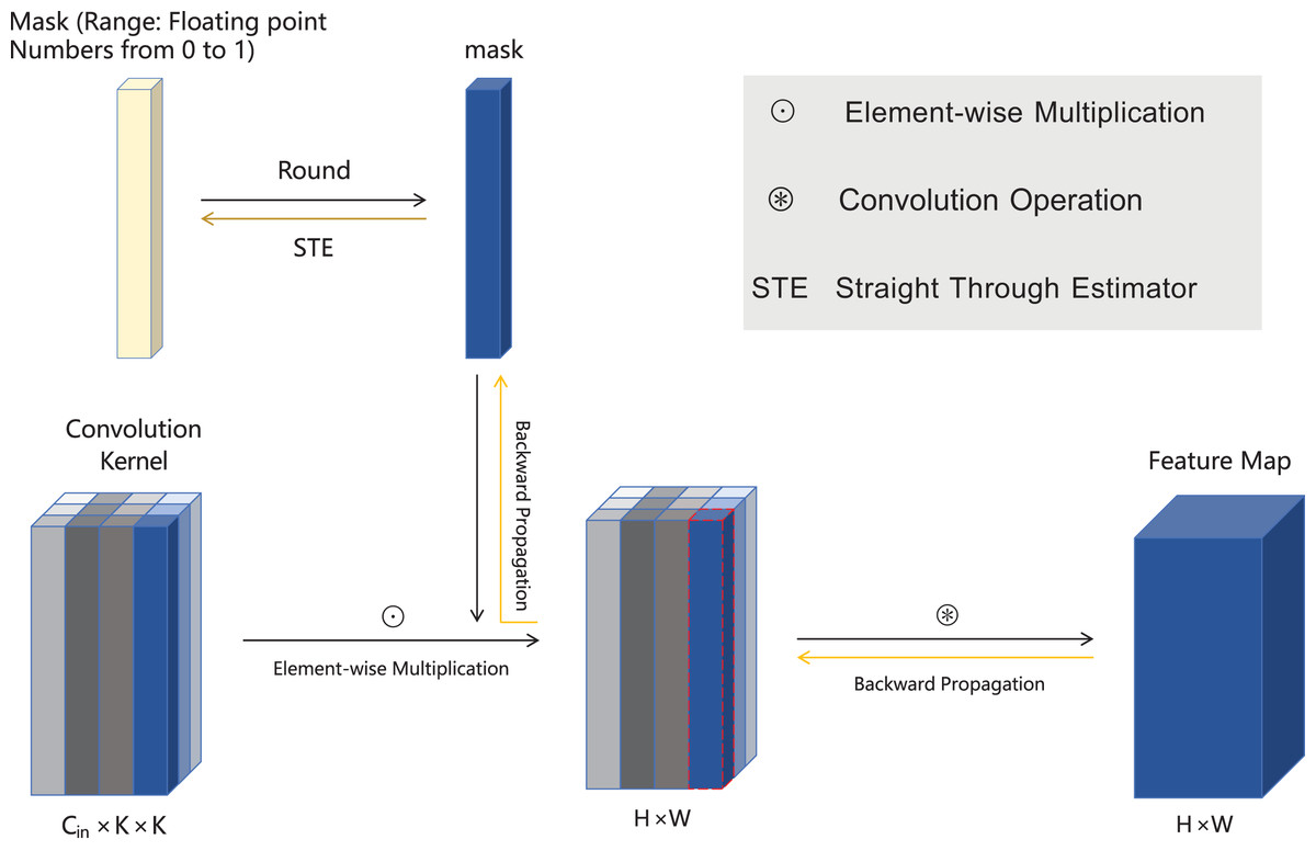
Figure 1: The framework of MLPrunner method.
For better representation, we have chosen one of the channels for description. Our method assigns a learnable mask to the channel, performs a round operation on the mask using a pre-defined pruning rate, and multiplies it with the weight W to determine whether the channel needs to be pruned. Then, a feature map is generated through convolution operation to determine the model. (Note: Considering the non differentiable nature of the round function, which prevents the gradient accepted by mask from being updated in a timely manner, we have adopted STE for backpropagation to solve this problem).
Mask forward. During forward propagation within a specific layer , we leverage the mask to obtain a binary indicator that guides the removal or preserve of corresponding filters. This is achieved using a pre-defined pruning rate to round to 0 or 1 s, where 0 indicate pruning corresponding weights, and vice versa. Formally, we first accumulate in a filter-wise manner as:
(5)
Then, the binary indicator is derived as
(6)
Finally, we use the binary indicator to prune the dense weights during forward propagation as:
(7) where denotes the point-wise multiplication.
Mask backward. The above forward phase enables automatic filter pruning by looking at value of mask , yet Eq. (7) is non-differentiable due to the round operation, making the mask unable to be updated, i.e., the gradient can not passed from to . To address this, we use the straight-through estimator (STE) (Bengio, Léonard & Courville, 2013) as an alternative to approximate the mask gradient of as:
(8)
In this manner, the mask can be jointly optimized with the weight during training. Notably, such mask learning process brings no gradient distortion to the weights as traditional training-aware pruning methods do. Furthermore, such learned masks can well tell the importance of corresponding filters, which we analyze below.
Tractability of optimization. We take a specific filter to show that our learned mask score can well reflect the relative importance of filter weights.
Omitting the update schedule including learning rate and momentum, we can represented the learned mask as
(9) where T denotes the total training iterations.
Now, let us turn our focus to the loss variation when removing . It can be derived using the Taylor expansion (Molchanov et al., 2017) as
(10) which leads Eq. (9) to
(11)
Here we can observe that the trained mask is the accumulation of loss change for removing weights . A small score denotes less loss increase thus the corresponding candidate can be safely removed. Thus, our introduced mask learning can be used to measure the relative importance between convolution filters, and preserving filters with larger mask value can well decrease the loss after pruning. The learned masks directly correlate with filter importance through the accumulated loss gradient Eq. (9). Unlike weight-penalty methods that distort gradients via L2 regularization, MLPruner’s masks provide unbiased importance estimates while preserving original weight optimization.
The overall pipeline of MLPruner is outlined in Algorithm 1. In particular, we set a mask training epochs to learn the masks for filter pruning. After that, we stop optimizing masks and obtain the pruned weight by extracting the corresponding filter from according to the binary indicator . Finally, we fine-tune the pruned model to further recover its performance. It can be inferred that MLPruner does not bring any weight penalty during training, but automatically learns masks that can well reflect the importance of filters with respect to the training loss, achieving holistic filter pruning in an end-to-end manner. MLPruner fundamentally differs from weight-penalty approaches in three ways: (1) Our masks provide unbiased importance estimates without distorting weight gradients as directly measures ’s true contribution to loss minimization, uncontaminated by auxiliary penalties, (2) The pruning decision is based on accumulated loss impact rather than instantaneous magnitude, and (3) We maintain the original training objective without additional regularization terms, delivering better generalization ability as weight updates follow the original loss gradient (Eq. 10), maintaining the model’s intrinsic generalization dynamics.
| Input: An L-layer CNN with weight , mask training epochs |
| Output: The pruned model weight |
| // Joint mask and weight training |
| 1 for do |
| 2 for each training iteration do |
| 3 Get binary indicator via Eqs. (6) and (5); |
| 4 Forward propagation via Eq. (7); |
| 5 Backward propagation via Eq. (8); |
| 6 end |
| 7 end |
| // Obtain the pruned weights |
| 8 for do |
| 9 = squeeze( ) // squeeze () denotes extract non-zero filters |
| 10 end |
| 11 Fine-tune to recover performance. |
Remark. In our description of MLPruner, we take the layer-wise pruning rate to be a known quantity. In practical scenarios, we can employ global sorting for the learned mask to acquire the binary indicator for each layer. In such case, the layerwise pruning rate is automatically derived, thereby showcasing the ease-of-use proffered by MLPruner. Furthermore, it is also worth noting that the existing structure-searching pruning methods (Lin et al., 2020c; Liu et al., 2019) hold orthogonality to MLPruner, which means that we could utilize the pruning rates identified from each layer to locally sort the mask and obtain the binary indicator. We manifest the comparative performance achieved through diverse layerwise pruning rates in the experiment section.
Experiment
Experimental settings
Datasets and networks. We conducted experiments on representative image classification datasets CIFAR-10, CIFAR-100 (Krizhevsky & Hinton, 2009), and ImageNet (Deng et al., 2009) to demonstrate the effectiveness of the proposed MLPruner. CIFAR-10 is comprised of 60,000 distinct 32 × 32 color images, spread evenly across 10 various classes, with each class housing 6,000 images. The CIFAR-100 dataset, designed parallel to CIFAR-10, departs only in its increased class count, featuring 100 distinct classes, each containing 600 images. We elect representative convolutional networks to validate the efficacy of MLPruner, including VGGNet-16 (Simonyan & Zisserman, 2015), GoogLeNet (Szegedy et al., 2015), ResNet (He et al., 2016), and MobileNet-V2 (Sandler et al., 2018).
Implementation details. We set the mask training epochs for CIFAR-10/100 and for ImageNet, with all masks initialized to 1s. After training masks, we directly conduct global sort on the masks to obtain layer-wise pruning rates and then prune filters based on the learned masks. All our pruned models are fine-tuned employing the stochastic gradient descent (SGD) optimizer, paired with a momentum of 0.9 and a batch size of 256. On CIFAR-10, Each pruned network is fine-tuned for 300 epochs, incorporating a weight decay factor of 10−3 and an initial learning rate of 0.1. This rate undergoes a subsequent reduction to 0.01 and then to 0.001 after specific intervals of 50 and 100 epochs respectively. On ImageNet, we give 90 epochs for tine-tuning with weight decay of 10−4. The learning rate is initialized to 0.1 and decayed by cosine annealing schedule. Besides, we employ random crop and horizontal flip to the input images. All experiments is implemented based on PyTorch and executed on NVIDIA 3090 GPUs.
Performance metrics and baselines. MLPruner is juxtaposed with several state-of-the-art pruning methods (He, Zhang & Sun, 2017; Huang & Wang, 2018; Li et al., 2017; Lin et al., 2020a, 2020c, 2019; Yu et al., 2018; Zhao et al., 2019). We report the top-1 accuracy to facilitate a quantitative comparison among various methods. The computing costs and storage demands are reflected in the number of FLOPs and parameters, accompanied by their corresponding pruning rates (PR), forming the basis for assessing the efficacy of our MLPruner and other methods used for comparison.
CIFAR-10
VGGNet-16. We first incorporate our MLPruner to prune the 16-layer VGGNet model, a classic CNN comprising 13 sequential convolutional layers and 3 fully-connected layers. Evident from Table 1, MLPruner markedly surpasses the current state-of-the-art methods across all performance indicators. Our MLPruner accomplishes a parameter compression of , thereby enhancing the computation by 71.9% along with a negligible accuracy decrease of 0.03%. This substantial improvement proves instrumental in deploying the VGGNet model on resource-restricted devices.
| Model | Top-1 (%) | FLOPs (PR) | Parameters (PR) |
|---|---|---|---|
| Baseline | 93.02 | 314.04M (0.0%) | 14.73M (0.0%) |
| SSS (Huang & Wang, 2018) | 93.02 | 183.13M (41.6%) | 3.93M (73.8%) |
| Zhao et al. (2019) | 93.18 | 190.00M (39.1%) | 3.92M (73.3%) |
| GAL-0.05 (Lin et al., 2019) | 92.03 | 189.49M (39.6%) | 3.36M (77.6%) |
| HRank (Lin et al., 2020a) | 92.34 | 108.61M (65.3%) | 2.64M (82.1%) |
| ABC (Lin et al., 2020c) | 92.51 | 92.45M (70.6%) | 1.75M (88.2%) |
| RGP (Chen et al., 2023) | 92.76 | 78.8M (74.89%) | 3.68M (75.00%) |
| MLPruner | 92.99 | 87.98M (71.9%) | 1.62M (89.1%) |
GoogLeNet. We further demonstrate the effectiveness of MLPruner in pruning GoogLeNet, a prevailing network with inception structure. Table 2 substantiates that notwithstanding marginal drops in top-1 accuracy (94.78% for MLPruner vs. 95.03% for the baseline), MLPruner significantly curtails the FLOPs by 62.5% and parameters by 61.3%. When juxtaposed with the superior state-of-the-art, i.e., HRank, MLPruner not only surpasses in accuracy performance but also substantially reduces the quantity of FLOPs and parameters. Consequently, MLPruner excels in diminishing the superfluity of networks with intricate multi-branch structures.
| Model | Top-1 (%) | FLOPs (PR) | Parameters (PR) |
|---|---|---|---|
| Baseline | 95.03 | 1.53B (0.0%) | 6.17M (0.0%) |
| (Li et al., 2017) | 94.54 | 1.02B (32.9%) | 3.51M (42.9%) |
| GAL-0.05 (Lin et al., 2019) | 93.93 | 0.94B (38.2%) | 3.12M (49.3%) |
| HRank (Lin et al., 2020a) | 94.53 | 0.69B (54.9%) | 2.74M (55.4%) |
| ABC (Lin et al., 2020c) | 94.55 | 0.71B (53.9%) | 2.89M (52.1%) |
| RGP (Chen et al., 2023) | 94.61 | 0.54B (64.8%) | 2.55M (58.7%) |
| MLPruner | 94.78 | 0.59B (62.5%) | 2.45M (61.3%) |
ResNet. We also evaluate the network pruning performances of various methods on ResNet (He et al., 2016), a predominant deep CNN with residual modules, as shown in Table 3. Notably, our MLPruner enhances the original ResNet-56 performance by 0.05%, successfully eliminating approximately 54.8% of FLOPs. This efficiency contrasts sharply with other methods, which invariably experience an accuracy reduction to varying degrees, despite achieving fewer reductions in FLOPs. Furthermore, our MLPruner exhibits remarkable superiority when applied to ResNet-110. Despite a robust 65.8% reduction in FLOPs, it generates a performance improvement of 0.08%, significantly outpacing competing methods.
| Model | Top-1(%) | FLOPs (PR) | Parameters (PR) |
|---|---|---|---|
| ResNet-56 | 93.26 | 126.56M (0.0%) | 0.85M (0.0%) |
| (Li et al., 2017) | 93.06 | 90.90M (27.6%) | 0.73M (14.1%) |
| GAL-0.6 (Lin et al., 2019) | 92.90 | 78.30M (37.6%) | 0.75M (11.8%) |
| FPGM (He et al., 2019) | 93.26 | 59.40M (52.6%) | – |
| ABC (Lin et al., 2021) | 93.19 | 73.36M (41.5%) | 0.50M (41.2%) |
| LFPC (He et al., 2020) | 93.24 | 59.10M (52.9%) | – |
| HRank (Lin et al., 2020a) | 93.17 | 62.72M (50.0%) | 0.49M (42.4%) |
| RGP (Chen et al., 2023) | 92.92 | 57.99M(54.2%) | 0.47M (44.8%) |
| MLPruner | 93.31 | 57.23M (54.8%) | 0.43M (49.5%) |
| ResNet-110 | 93.57 | 254.99M (0.0%) | 1.73M (0.0%) |
| (Li et al., 2017) | 93.30 | 155.00M (38.7%) | 1.16M (32.6%) |
| GAL-0.5 (Lin et al., 2019) | 92.55 | 130.20M (48.5%) | 0.95M (44.8%) |
| HRank (Lin et al., 2020a) | 93.36 | 105.70M (58.2%) | 0.70M (59.2%) |
| LFPC (He et al., 2020) | 93.07 | 101.00M (60.3%) | – |
| ABC (Lin et al., 2020c) | 93.44 | 92.84M (63.3%) | 0.69M (59.9%) |
| RGP (Chen et al., 2023) | 93.51 | 91.59M (64.1%) | 0.63M (63.7%) |
| MLPruner | 93.65 | 87.11M (65.8%) | 0.61M (64.8%) |
MobileNet. MobileNet-v2 (Sandler et al., 2018), an advancing network, exemplifies compact design via its depth-wise separable convolution. Given its minuscule computational cost, pruning MobileNet-v2 proves to be an exceptionally challenging task. Nevertheless, as illustrated in Table 4, in comparison with its competitors, MLPruner impressively maintains a superior top-1 accuracy of 95.31%, whilst achieving a more significant pruning of FLOPs by 31.5%. Therefore, the results underscore the notable preeminence of our MLPruner in CNN pruning, unflinchingly handling even highly compact network models.
| Model | Top-1 (%) | FLOPs (PR) | Parameters (PR) |
|---|---|---|---|
| Baseline | 94.47 | 98.05M (0.0%) | 2.29M (0.0%) |
| WM (Howard et al., 2017) | 94.02 | 71.57M (27.0%) | 1.81M (20.9%) |
| DCP (Zhuang et al., 2018) | 94.69 | 71.57M (27.0%) | 1.81M (20.9%) |
| MDP (Guo, Ouyang & Xu, 2020) | 95.14 | 69.90M (28.7%) | – |
| White-Box (Zhang et al., 2022) | 95.28 | 69.41M (29.2%) | 1.77M (22.3%) |
| MLPruner | 95.31 | 67.16M (31.5%) | 1.56M (23.4%) |
CIFAR-100
We further demonstrate the efficacy of MLPruner for pruning VGGNet-19 on the more complex dataset CIFAR-100. Table 5 shows the comparative performance of MLPruner under analogous pruning rates vs. other methodologies. Observable from these comparisons, MLPruner outperforms the state-of-the-art (SOTA) alternatives across varying pruning rates. Emphasizing further, MLPruner successfully minimizes the FLOPs to a fraction of 70.7%, simultaneously achieving a top-1 accuracy of 73.45%. Conversely, the recent SOTA, HRank (Lin et al., 2020a), demands greater computation to yield subpar top-1 accuracy at 72.91%. Undeniably, these results accentuate the distinct advantage of employing our MLPruner in pruning CNNs on more challenging datasets.
| Model | Top-1 (%) | FLOPs (PR) | Parameters (PR) |
|---|---|---|---|
| Baseline | 73.43 | 399.12M (0.0%) | 20.04M (0.0%) |
| (Li et al., 2017) | 72.52 | 171.51M (42.9%) | 5.17M (74.2%) |
| HRank (Lin et al., 2020a) | 72.91 | 154.06M (61.4%) | 4.08M (80.2%) |
| ABC (Lin et al., 2020c) | 73.04 | 145.67M (63.5%) | 3.54M (82.3%) |
| White-Box (Zhang et al., 2022) | 73.33 | 127.31M (68.1%) | 2.38M (86.4%) |
| MLPruner | 73.45 | 116.94M (70.7%) | 2.18M (88.1%) |
ImageNet
In the challenging ImageNet dataset, we compared MLPruner with current state-of-the-art pruning technologies. Key performance indicators, as observed in Table 6, reveal that MLPruner demonstrates a significant advantage in many core metrics. Firstly, MLPruner achieved a Top-1 accuracy of 75.62%, which not only surpasses most of the listed methods such as White-Box, DSA, and CLR-RNF—with accuracies of 75.32%, 75.10%, and 74.85%, respectively—but also shows considerable improvements over ThiNet at 72.04% and GAL at 71.95% Top-1 accuracy. This enhancement is particularly crucial as it demonstrates the capability to balance the reduction of computational resources while maintaining model performance during the pruning process. Further, MLPruner outperforms EagleEye by 1.2% accuracy at similar FLOPs because: (1) Our mask learning adapts to training dynamics rather than using fixed heuristics, (2) Joint optimization prevents the greedy local decisions EagleEye makes, and (3) The gradient-based importance measure better preserves critical filters.
| Model | Top-1 (%) | FLOPs (PR) | Parameters (PR) |
|---|---|---|---|
| Baseline | 76.15 | 4.10G (0%) | 25.56M (0%) |
| ThiNet (Luo, Wu & Lin, 2017) | 72.04 | 1.62G (60.2%) | 14.55M (43.0%) |
| SFP (He et al., 2018a) | 74.61 | 2.38G (58.2%) | – |
| GAL (Lin et al., 2019) | 71.95 | 2.33G (43.0%) | 21.25M (16.9%) |
| HRank (Lin et al., 2020a) | 74.98 | 2.29G (44.1%) | 16.17M (36.7%) |
| White-Box (Zhang et al., 2022) | 75.32 | 2.23G (45.5%) | 16.49M (35.5%) |
| DSA (Ning et al., 2020) | 75.10 | 2.46G (40.0%) | – |
| CLR-RNF (Lin et al., 2022) | 74.85 | 2.44G (40.3%) | 16.91M (33.8%) |
| MLPruner | 75.62 | 2.21G (46.0%) | 14.47M (43.4%) |
| EagleEye (Li et al., 2020) | 76.40 | 2.00G (51.2%) | – |
| Pas (Li et al., 2022) | 76.70 | 2.00G (51.2%) | – |
| MLPruner | 76.89 | 1.97G (51.9%) | 13.98M (45.6%) |
Moreover, in terms of computational efficiency, MLPruner’s performance is equally impressive. It reduced the total number of floating-point operations (FLOPs) by 46.0%, achieving only 2.21G. This figure is not only lower than the baseline model’s 4.10G but also slightly better compared to other methods like DSA’s 2.46G and CLR-RNF’s 2.44G, indicating that MLPruner effectively lessens the computational load while preserving a relatively high accuracy. To sum up, Compared to other pruning methods, MLPruner not only reduces parameters more efficiently but also maintains better performance, even on more challenging dataset.
We conclude with a discussion on the pruning efficiency. Traditional methods, such as ThiNet and HRank, typically determine layer-wise pruning rates through manual design, which incurs significant human effort. On the other hand, search-based approaches, such as EagleEye and ABCPruner, often employ evolutionary algorithms or specific evaluation metrics to explore optimal architectures, which still demand substantial computational time. In contrast, our proposed MLPruner achieves automatic mask training with only one-tenth of the fine-tuning cost, enabling end-to-end optimization of both layer-wise pruning rates and critical filter identification, thereby enhancing pruning efficiency compared to existing methods.
Performance analysis
In this section, we prune ResNet-56 and test its performance on CIFAR-10 as an example to analysis the performance of MLPruner w.r.t. its different components.
Mask learning epochs. Initially, we scrutinize the import of learning epochs for masks. Figure 2 delineates the performance nuances when utilizing varying epochs at diverse pruning ratios. Manifestly, enhancing the epochs of mask learning significantly augments the model’s efficacy, particularly under conditions of high sparsity. This phenomenon is intuitively understandable as a higher sparsity demands the removal of multiple filters, thereby necessitating an amplified number of mask training epochs to discern the priority between diverse filters. Concurrently, it should be noted that the performance gains of increasing epochs possess a ceiling effect, and an abundance of epochs can incur inflated training overhead. Therefore, we configure the mask training for 30 epochs.
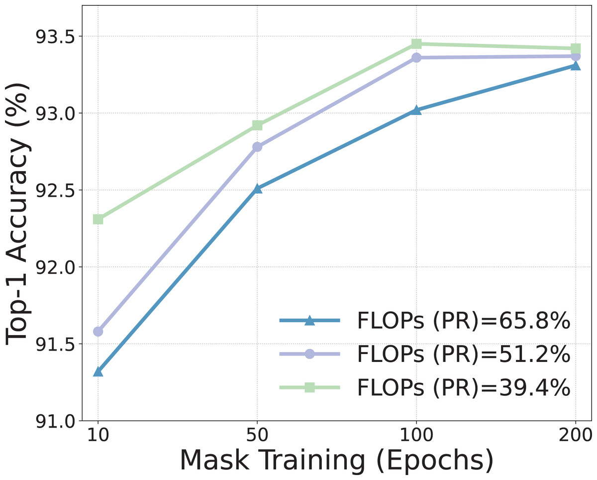
Figure 2: Effect of the mask learning epochs within MLPruner.
Layerwise pruning rate. We further investigated the impact of layerwise pruning rate on MLPruner’s performance. Table 7 exemplifies the effect on FLOPs reduction and overall performance when employing different strategies to distribute the layerwise pruning rate. Interestingly, direct global ranking based on the learned mask can even yield better results than a manually set procedure, which underscores MLPruner’s efficiency. Furthermore, the use of a searched layerwise pruning rate can lead to enhanced performance, albeit at increased costs. This demonstrates MLPruner’s scalability, remaining orthogonal to the pruning methods predicated on architecture search.
| Setting | Top-1 accuracy(%) | FLOPs(PR) |
|---|---|---|
| Manual | 93.02 | 53.3% |
| ABCPruner | 93.49 | 41.2% |
| Global | 93.31 | 54.8% |
Weight penalty. At last, we examine the impact of weight penalties on mask training within MLPruner, a widely adopted approach in training-aware filter pruning methods (Huang & Wang, 2018; Xiao, Wang & Rajasekaran, 2019). Specifically, we imposed an L1 penalty on the mask during its training course, with results displayed in Table 8. As can be seen, the introduction of a sparsity regularization term resulted in performance degradation. This can be attributed to the fact that our mask training strategy already accurately identifies critical filters, and the penalty item inevitably hinders the optimization of the mask.
| Setting | Top-1 accuracy(%) | FLOPs(PR) |
|---|---|---|
| w. Penalty | 92.89 | 53.9% |
| w.o. Penalty (MLPruner) | 93.31 | 54.8% |
Future work
In this section, we discuss some future works that warrant exploration. First, the current mask learning process in MLPruner relies on a fixed threshold for binarization, which may not optimally adapt to varying layer-wise pruning sensitivities. Future work could explore dynamic or learnable threshold mechanisms to enhance flexibility. Second, the method primarily focuses on filter pruning for CNNs, leaving room for extension to other architectures (e.g., transformers), particularly considering the structural differences in attention mechanisms and positional encodings. Third, the increased computational overhead during mask training requires optimization for larger-scale models. Fourth, while demonstrated on classification tasks, applicability to dense prediction tasks (e.g., segmentation) needs further validation. Lastly, the theoretical connection between mask values and filter importance could be further formalized to guide more principled pruning decisions. Addressing these limitations could broaden the applicability and robustness of the approach.
Conclusion
Filter pruning emerges as a research hotspot in both industrial and academic realms, intended to minimize the deployment and inference overhead of CNNs. In this article, we introduce a novel MLPruner methodology, which autonomously learns mask through threshold-based rounding forward and STE-based backward. The learned masks by MLPruner has been demonstrated to reflect a corresponding filter’s significance, even in the absence of weight penalty that previous methods impose. Extensive experiments highlights the effectiveness of MLPruner in pruning popular CNN architectures as compared to a series of state-of-the-art filter pruning methods.