
Apple estimation and recognition in complex scenes using YOLO v8
- Published
- Accepted
- Received
- Academic Editor
- Davide Chicco
- Subject Areas
- Algorithms and Analysis of Algorithms, Artificial Intelligence, Computer Vision, Data Mining and Machine Learning, Neural Networks
- Keywords
- Natural environment, Apple estimation, Apple detection, Color space transformation, YOLO v8
- Copyright
- © 2025 Geng et al.
- Licence
- This is an open access article distributed under the terms of the Creative Commons Attribution License, which permits unrestricted use, distribution, reproduction and adaptation in any medium and for any purpose provided that it is properly attributed. For attribution, the original author(s), title, publication source (PeerJ Computer Science) and either DOI or URL of the article must be cited.
- Cite this article
- 2025. Apple estimation and recognition in complex scenes using YOLO v8. PeerJ Computer Science 11:e3116 https://doi.org/10.7717/peerj-cs.3116
Abstract
Apple-picking robots are designed to accurately identify ripe apples, efficiently harvest them, and offer adaptable solutions applicable to various fruits. However, current methods show limited detection accuracy in complex environments due to challenges such as shading in natural settings, variations in ambient lighting, and diversity in fruit color, shape, and size. This study integrates Hue–Saturation–Value (HSV) color space transformation with YOLO v8 models to identify the quantity and location of apples, while also assessing their ripeness and weight. First, image data of apples in natural environments were collected and preprocessed using grayscale conversion and Gaussian filtering for denoising. Next, edge detection was performed using the Canny and Sobel algorithms, and apple counting was achieved via the YOLO v8 model. Ripeness was evaluated based on HSV and Red–Green–Blue (RGB) values, while weight estimation was conducted by constructing 3D models of the fruits. Finally, through color feature extraction and YOLO v8, apples were precisely identified among various fruits. Experimental results show that the YOLO v8 model achieved an average precision of 95% and an F1-score of 93.45%. Compared to existing algorithms such as Visual Geometry Group (VGG) and Residual Network (ResNet), YOLO v8 improved Mean Average Precision (mAP) by 0.14% and 8%, respectively. These advancements provide strong technical support for apple-picking robots, enabling faster and more accurate operations, improving fruit quality, and meeting the practical demands of agricultural production.
Introduction
As the world’s largest apple producer and exporter, China’s annual output is approximately 35 million tons (Zhao, 2019). Apples are rich in vitamins and minerals. As a wealthy industry, its high-quality development has become the basis for promoting regional rural revitalization industries. With the popularization of agricultural mechanization, the application of intelligent machinery is becoming increasingly extensive in agricultural production, which effectively reduces the dependence on manpower in the process of apple picking, thus significantly improving picking efficiency (Zhang et al., 2020; Chu et al., 2021). However, mechanical picking faces many challenges in the identification and estimation of apples. In real production, there are many interference factors such as fruit occlusion and light changes. Therefore, to solve key problems such as labor cost savings, fruit damage rate reduction and picking efficiency improvement (Song, Shang & He, 2023), it is of great practical importance and broad application prospects to use deep learning technology to achieve accurate identification and positioning of apples in complex environments.
The target recognition algorithms in deep learning can be divided into two categories: two-stage target detection and one-stage target detection. The two-stage target detection method generates candidate target regions through the region proposal network and classifies and bounding boxes regresseses the candidate regions to obtain accurate target locations and categories. Examples of algorithms within this category include Region-based Convolutional Neural Network (R-CNN) (Girshick et al., 2015), Fast R-CNN (Girshick, 2015), Faster R-CNN (Ren et al., 2017). On the other hand, the one-stage target detection method directly predicts the category and location of the target on the image without generating candidate regions. This method is suitable for problems that require real-time target detection and positioning, especially in scenarios with high-speed requirements, such as real-time obstacle detection in autonomous driving, pedestrian detection in monitoring systems, and product quality inspection in industrial applications. These scenarios need to quickly and accurately detect the location and category of a single target, and the single target detection method can directly predict without generating candidate regions. Examples of algorithms within this category include You Only Look Once (YOLO) (Redmon et al., 2016), Single Shot Multi-Box Detector (SSD) (Liu et al., 2016), RetinaNet (Cheng & Yu, 2020). However, SSD relies on a fixed set of default anchor boxes and scale assignments, which limits its localization accuracy for small or densely clustered objects, and often results in missed detections under complex backgrounds. RetinaNet introduces the focal loss to address class imbalance but still depends on predefined anchors and employs a heavier backbone network, leading to reduced inference speed and sensitivity to occlusion and background clutter. In contrast, our proposed network leverages adaptive anchor assignment and enhanced feature-pyramid fusion to maintain high detection precision and real-time performance across multiple targets, even in the challenging, multi-object scenarios typical of orchard environments.
As a new network model that has attracted much attention in recent years, the YOLO algorithm has obvious advantages in terms of detection speed and accuracy and has been widely used in many fields such as industry, agriculture and transportation. With its continuous evolution and improvement, the YOLO algorithm has successively introduced multiple versions including YOLO v3 (Alsanad et al., 2022), YOLO v4 (Wu et al., 2023), and YOLO v5 (Ghose et al., 2024). As the latest evolutionary version of the YOLO algorithm, YOLO v8 (Talaat & ZainEldin, 2023) continues to have rapid detection speed and excellent detection accuracy.
Although several YOLO variants, v9 (Wang, Yeh & Liao, 2024), v10 (Wang et al., 2024), v11 (Khanam & Hussain, 2024) and v12 (Tian, Ye & Doermann, 2025), have been released since v8, each presents trade-offs that limit its suitability for real-time, edge-based orchard applications. Specifically, YOLO v9 (Wang, Yeh & Liao, 2024) implemented additional architectural pruning to increase throughput but experienced a significant decline in small- recognition accuracy in dense orchard scenes; its higher computational cost (112 GFLOPs compared with v8’s 85 GFLOPs) also led to an 18% reduction in frame rates on identical hardware. YOLO v10 (Wang et al., 2024) introduced dynamic depth-and-width scaling to increase flexibility; however, it exhibited unstable convergence across heterogeneous field data and required extensive retraining, with [email protected] falling to 0.75 under more than 50% occlusion—an important shortcoming for dense apple clusters. YOLO v11 (Khanam & Hussain, 2024) integrated transformer-based attention heads to capture long-range context but the resulting increase in model size and memory footprint impeded real-time inference on lightweight devices, and its reliance on over 10 million pretraining images proved impractical for smaller orchards with limited annotations. Finally, YOLO v12 (Tian, Ye & Doermann, 2025) refined feature maps through spatial–channel attention modules but incurred higher inference latency and doubled video random-access memory (VRAM) requirements (8 GB vs 4 GB for v8), offsetting potential speed gains in robotic picking systems. Taken together, these findings indicate that despite their respective enhancements, further optimization of advanced YOLO variants is necessary to satisfy the stringent speed, accuracy and resource constraints of automated orchard deployments.
In complex orchard environments, the presence of multiple overlapping fruits, variable lighting and background clutter can significantly degrade detection performance. Benchmark studies report that single-object detection in controlled settings often exceeds 95% accuracy (Tarkasis, Kaparis & Georgiou, 2025), whereas accuracy can fall below 80% when multiple targets and complex textures are present (Huang et al., 2024). To address these challenges, preprocessing methods such as image binarization, which separates foreground fruit from background noise, and edge detection, which emphasizes object contours, have been shown to improve multi-object detection robustness (Yi et al., 2025; Ahmed & Jalal, 2024). In particular, binarization reduces false positives by isolating high-intensity fruit regions, and edge detection enhances boundary clarity, facilitating accurate localization in cluttered scenes.
Several classical edge-detection operators have been proposed to highlight object boundaries in images. The Roberts operator computes diagonal gradients using simple 2 × 2 kernels, offering low computational cost but producing noisy, fragmented edges (Canny, 1986). The Prewitt operator extends this approach to horizontal and vertical directions with slightly larger kernels, improving noise resilience at the expense of blurred contours in high-contrast scenes (Sobel & Feldman, 2015). The Laplacian of Gaussian detects edges by finding zero-crossings in the second derivative, yielding continuous boundaries, but often amplifying spurious responses in textured backgrounds (Xie & Tu, 2015). In contrast, the Sobel operator combines Gaussian smoothing and first-derivative convolution in orthogonal directions to generate robust gradient maps, effectively capturing local intensity transitions while suppressing high-frequency noise (Zhang et al., 2024). The Canny method refines these results through a multi-stage process consisting of Gaussian blur, gradient magnitude and orientation computation, non-maximum suppression and dual thresholding, producing clean, continuous contours with minimal background interference (Kong et al., 2023). Given these characteristics, we adopted Sobel and Canny edge detection in our preprocessing pipeline. Sobel quickly emphasizes prominent intensity changes to reveal coarse object outlines, while Canny produces precise, noise-reduced contours. Together, binarization and edge-enhancement steps strengthen YOLO v8’s ability to localize and identify apples under complex orchard conditions.
To provide a fair comparison, we selected Visual Geometry Group (VGG) (Pandiyaraju et al., 2025), Residual Network (ResNet) (Wu et al., 2025) and MobileNet (Wijayanto, Swanjaya & Wulanningrum, 2024) as alternative backbones, each adapted for object detection by appending comparable detection heads. VGG’s (Pandiyaraju et al., 2025) uniform 3 × 3 convolution stacks have been widely used in both single- and two-stage detectors with feature-pyramid modules. ResNet (Wu et al., 2025) introduces residual connections to enable deeper representations and serves as a backbone in Faster R-CNN and SSD frameworks. MobileNet (Wijayanto, Swanjaya & Wulanningrum, 2024) employs inverted residuals and linear bottlenecks to achieve a lightweight architecture suitable for edge-device deployment (e.g., MobileNet-SSD). By training all models under identical conditions, we ensure that our head-to-head evaluation against YOLO v8 fairly reflects each backbone’s detection capability.
Building on these insights, our study uses YOLO v8 as the baseline detection framework and augments it with targeted preprocessing and modeling strategies for real-world orchard applications (Ni et al., 2020; Wan et al., 2018; Parvathi & Selvi, 2021). We first applied grayscale scaling and Gaussian filtering for noise reduction, followed by Canny and Sobel edge detection to enhance contour clarity. The processed images were then used to train the YOLO v8 model to detect apple instances and their positions. Ripeness assessment was performed via Hue–Saturation–Value (HSV) and Red–Green–Blue (RGB) color-space analysis, and fruit weight was estimated through 3D reconstruction of detected apples. This integrated approach combining color feature transformation with YOLO v8’s real-time performance yields an efficient, robust apple localization and estimation model that addresses complex orchard challenges and lays the groundwork for future hardware-deployment studies.
Materials and Methods
Image dataset
This study utilized a diverse dataset comprising 20,853 images under varying lighting conditions, shooting angles, and fruit quantities, as detailed in Appendix 1 and https://github.com/gbbei-hui/test (2023 APMCM Asia-Pacific Contest Problem A: Data Materials for Image Recognition in Fruit-Picking Robots). Specifically, 11,144 apple images were sourced from the internet, captured in natural environments, while 200 images depicted scenes with apples placed on tree trunks at different angles and distances, as illustrated in Figs. 1A–1D. Additionally, the dataset included 2,028 images of starfruit, 3,012 of pears, 2,298 of plums, and 2,171 of tomatoes.
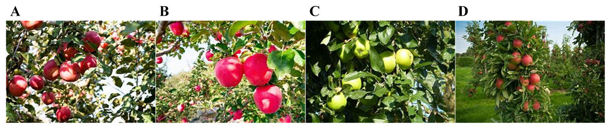
Figure 1: Image acquisition of the apples under multiple backgrounds.
(A) Different light exposures, (B) different fruit sizes, (C) similar colors of fruits and leaves, and (D) fruits occluded by leaves.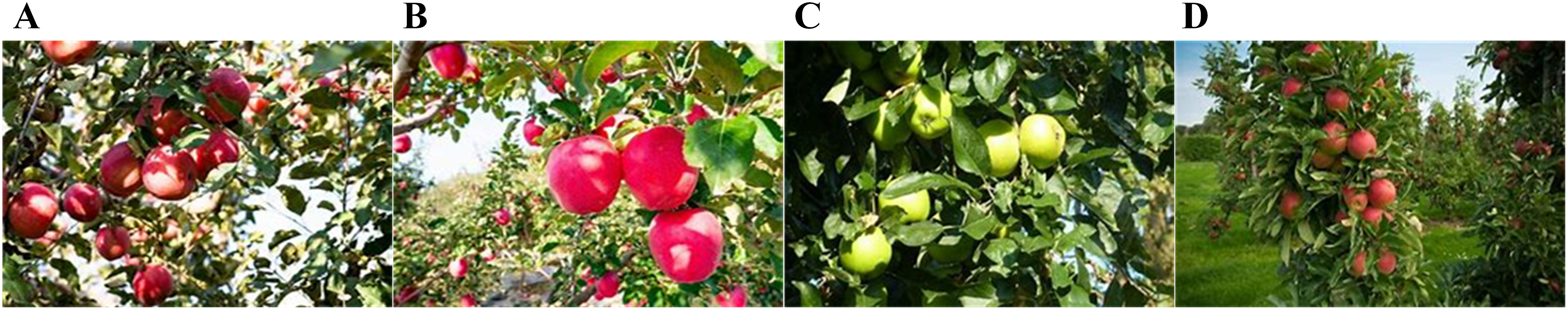
The processed data, shown in Figs. 2A–2E, were used to train the YOLO v8 model, enabling it to recognize the five fruit types listed in https://github.com/gbbei-hui/test (2023 APMCM Asia-Pacific Contest Problem A: Data Materials for Image Recognition in Fruit-Picking Robots). During training, multiple iterations and result adjustments were conducted to determine the optimal model weight parameters. The trained model was then applied to 20,000 images in Appendix 3 for practical recognition tasks. Through further pixel-level feature extraction, the deep learning model accurately identified valuable information, ensuring precision and reliability in recognition.
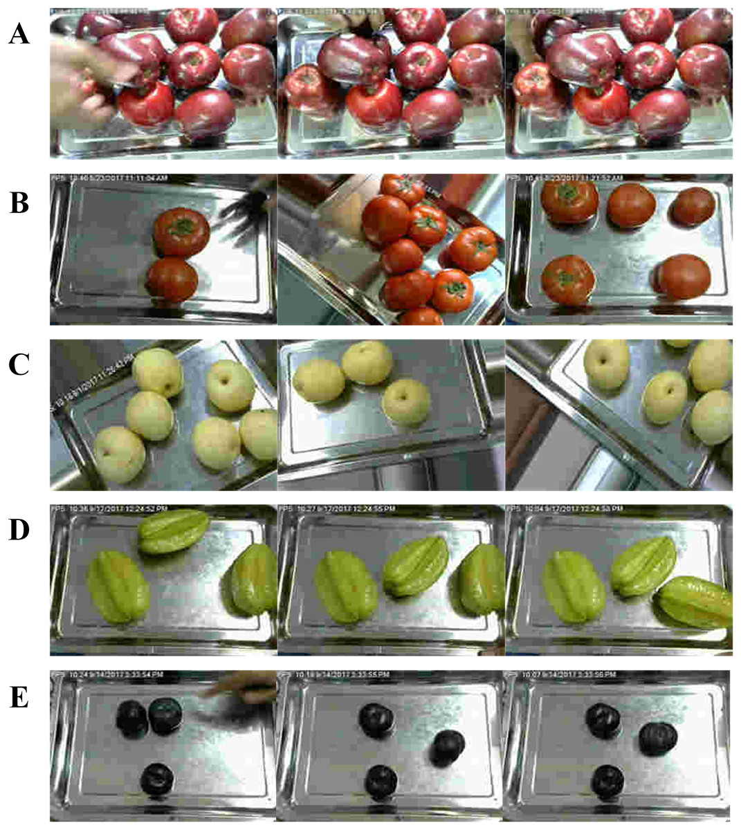
Figure 2: Sample images of five fruits.
(A) A large number of apples in multiple directions and with occlusion, (B) tomatoes with a high degree of similarity in shape and color to apples, (C) pears with similar characteristics except for different colors from apples, (D) carambola with apples when they are not ripe, and (E) plums with similar shapes and colors to apples under backlight.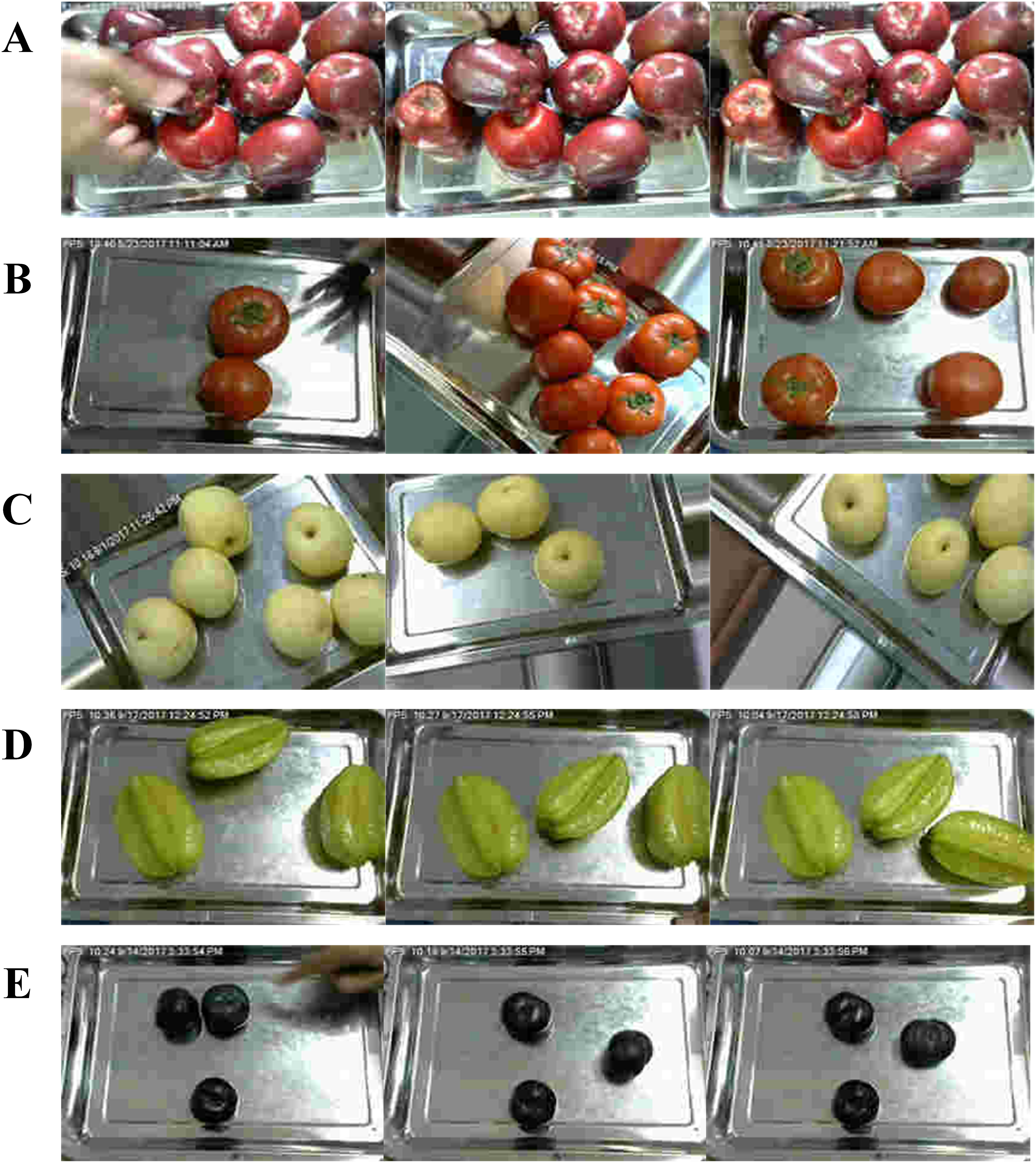
As shown in Table 1, to ensure robust training and evaluation of the YOLO v8 model, the full dataset was partitioned into training, validation and test sets in an 8:1:1 ratio. We preprocessed the image data by resizing all images to 640 × 640 pixels and converting the color space from BGR to RGB. Subsequently, we normalized the images so that the sum of pixel values equals one, thereby enhancing color distribution features. After normalization, each RGB image was represented as a feature vector stored in a one-dimensional array. The dataset was meticulously curated to include images of apples and other fruits captured under various real-world conditions, ensuring the model’s adaptability to complex scenarios. These preprocessing steps provided a robust foundation for training the YOLO v8 model, enabling effective detection of apples in intricate backgrounds. The ultimate goal was to support the training and evaluation of the YOLO v8 model, ensuring its accuracy and reliability in practical applications.
| Dataset split | Number of images | Proportion |
|---|---|---|
| Train | 16,682 | 80% |
| Validation | 2,086 | 10% |
| Test | 2,085 | 10% |
| Total | 20,853 | 100% |
Data processing
The image data are processed through the processes of characterization, binarization, denoising, and open and closed operations to increase the image quality, highlight the target object (apple), and effectively reduce the interference of the complex background in apple recognition to improve the accuracy and efficiency of recognition. The combined use of the Sobel and Canny operators reduces the number of errors in edge detection and enhances the model’s ability to recognize apples under different backgrounds and lighting conditions, thus improving the model’s generalizability. To further enhance the model’s ability to recognize apples under different backgrounds and lighting conditions, Sobel and Canny operators are used in combination to reduce the errors in the edge detection process. This enhances the edge detection effect of the model and improves its generalization ability so that the model maintains stable recognition performance in diverse environments. To improve model compatibility, the default BGR color space was first converted to the RGB color space. The computer-recognized RGB image is subsequently converted to the HSV color mode, which is closer to human visual perception. This conversion effectively distinguishes the color of the target object from that of other objects and reduces visual interference. This series of preprocessing methods lays a solid foundation for subsequent model training and improves the recognition efficiency and accuracy of the apple.
Owing to the differences in the natures of the 200 images in the dataset, the pixels of the individual images are unified to increase the compatibility of the data and avoid potential error problems. The preprocessing process requires characterization, binarization, denoising, an open operation, a closed operation and other processing steps for each image. As shown in Figs. 3A and 3B, the original image of the apple is grayed first. The gray image generated by this method has only one channel, in which each pixel value represents the gray level of the corresponding position, to obtain comparable features, that is, the color image is converted into a gray image, which helps reduce the number of calculations and highlights the brightness information in the image. That is, the calculation formula of the color image to the grayscale image is as follows:
(1)
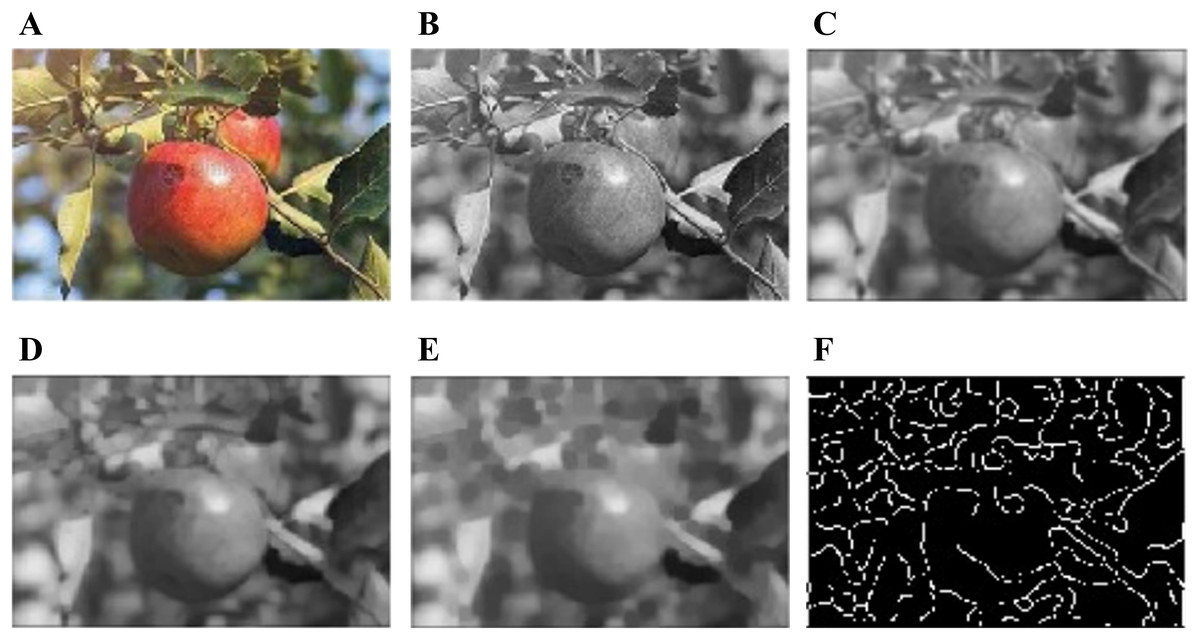
Figure 3: Apple image data enhancement.
(A) Original image, (B) greyscale image, (C) Gaussian filtered image, (D) opened image, (E) closed Image, and (F) edge detection image.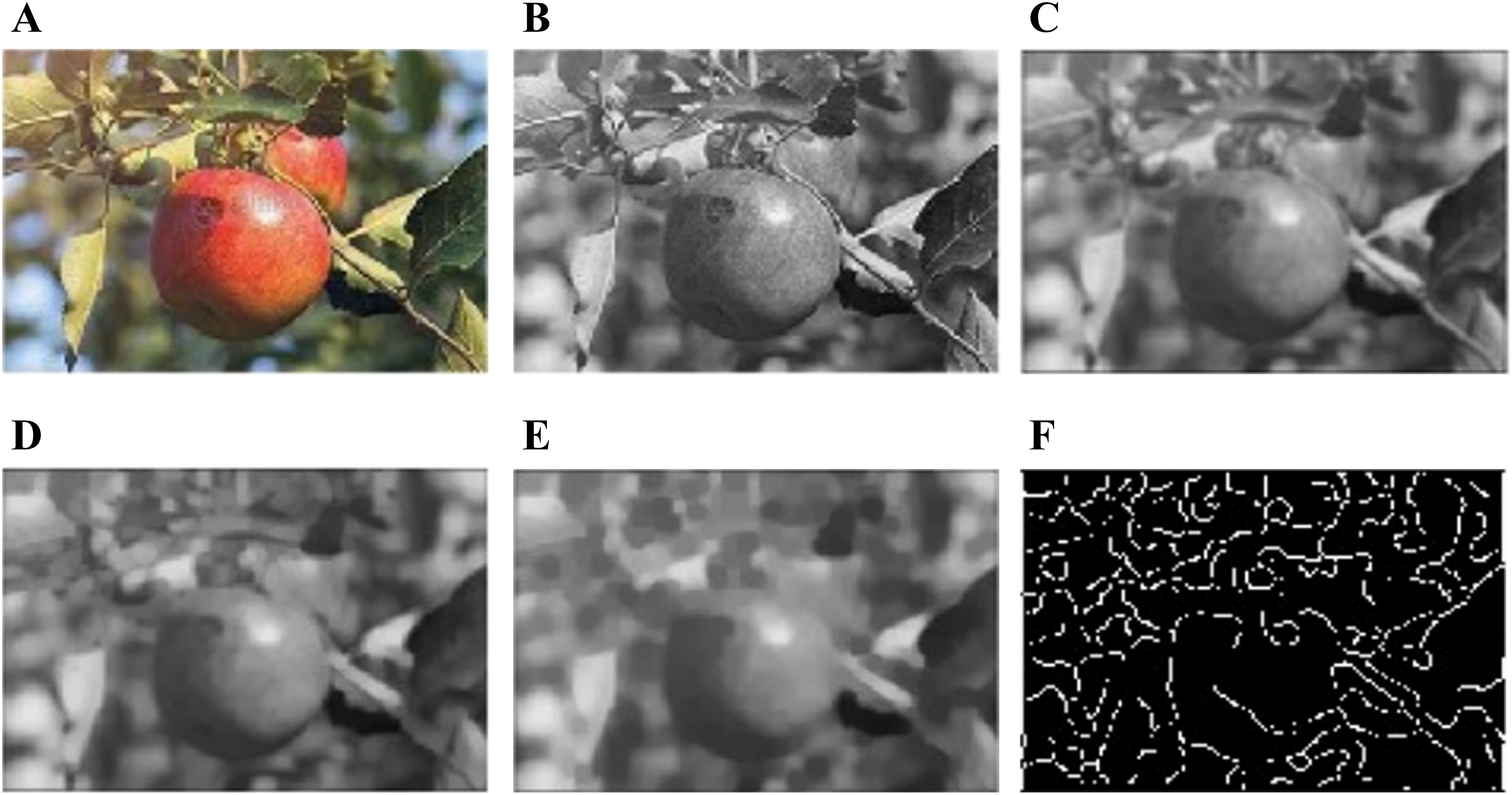
Grey represents a greyscale image, and RGB represents the greyscale values of the red, green, and blue channels of a colour image. The subsequent conversion of the image to a black-and-white binary image divides the pixels in the image into two categories, one that is given a value above the threshold and another that is assigned another value, which indicates that it is below the threshold. Figure 3C uses a Gaussian filter to remove random noise from the grayscale image to remove the noise in the image. The mathematical formula for a one-dimensional Gaussian filter is as follows:
(2)
The mathematical formula for the two-dimensional Gaussian filter (Matei & Chiper, 2024) is as follows:
(3) where is the standard deviation of the Gaussian distribution. The operation of first corroding and then expanding is used to separate the connections between adjacent objects in the image and smooth the object boundaries. Close operations, on the other hand, expand first and then corrode to connect the fractures between objects, making the objects in the image more compact.
In Figs. 3D and 3E, the open operation helps to repair small holes and cracks on the surface of the apple to further smooth the image boundaries and eliminate small objects and noise. Figure 3F uses Canny for edge detection, which accurately extracts the outline of the apple in the image by calculating the gradient intensity and direction of each pixel in the image and uses non-maximum suppression and double threshold detection to determine the edges. The Sobel operator and Canny operator were applied for edge detection to further improve the feature expression and accuracy of the image. These meticulous preprocessing steps provide a more reliable input database for training the model, which can help improve the model’s performance in processing apple estimation and recognition tasks.
Edge detection
In this study, we selected the Canny and Sobel operators (Onyedinma Ebele, Asogwa Doris & Onwumbiko Joy, 2025; Peng & Chaikan, 2021) for apple edge extraction because their complementary strengths, including precise contour localization achieved by the Canny operator’s noise-suppressed multi-stage detection and robust gradient computation provided by the Sobel operator’s effective filtering, enhance boundary clarity under varied lighting, occlusion and background complexity. Edge detection (Soria et al., 2023; Mittal et al., 2019) is crucial for distinguishing apples from surrounding textures and other objects, as it highlights structural features that improve the model’s ability to recognize and localize fruit.
In complex orchard scenes, apple edges were often obscured by leaves, branches or uneven illumination. The Canny operator addressed these challenges by first applying Gaussian blur to remove noise, then computing gradient intensity and orientation to identify edge candidates and finally using non-maximum suppression and double-thresholding to produce clean, continuous contours. This multi-stage process effectively suppressed background interference and yielded precise apple boundary outlines. Meanwhile, the Sobel operator calculated horizontal and vertical gradients of the grayscale image after Gaussian smoothing to measure pixel-value changes corresponding to edge transitions. By convolving the image with Sobel kernels in the x and y directions, we derived gradient amplitude and direction for each pixel. Applying an appropriate threshold then extracted clear edge maps, reinforcing apple regions and facilitating contour recognition by the YOLO v8 model.
These edge maps were incorporated into our preprocessing pipeline. Apple regions were first enhanced through Canny- and Sobel-based edge extraction, and the resulting feature-rich images were used to train YOLO v8 for recognition. The model parsed the output to locate apple bounding boxes, whose centers indicated fruit positions. This integrated approach improved detection accuracy and robustness in complex orchard environments, advancing precision agricultural monitoring and management.
Horizontal:
(4)
Vertical direction:
(5)
The Canny operator (Song, Zhang & Liu, 2017) is regarded as an efficient edge detection algorithm that first uses a Gaussian filter to denoise the image to reduce the influence of noise on edge detection. When calculating the image gradient, an advanced gradient detection operator is used, which uses a Gaussian filter to calculate the gradient, to obtain a smoother and more accurate gradient image. The Sobel operator is subsequently used to calculate the first derivatives (Gx and Gy) in the horizontal and vertical directions, respectively. Find the gradient and direction of the boundary on the basis of the two obtained gradients ( and ) via the following formula:
(6)
(7)
The algorithm uses non-maximum suppression technology to detect the local maximum value of pixels and sets the gray value corresponding to the non-maximum value to 0 to effectively filter out most of the non-edge pixels and retain the real edge information. Then, the Canny algorithm uses a double threshold strategy to connect the edges, using the high-threshold image to connect the edges into contours, and when the contours reach the endpoints, the algorithm looks for the points that meet the low-threshold conditions within eight neighborhoods of the point to generate new edges, and finally ensures the closure and continuity of the entire image edges.
HSV (Hue, saturation and value)
HSV (Stenger et al., 2019; Kurniastuti et al., 2022; Sari & Alkaff, 2020; Johari & Khairunniza-Bejo, 2022) color space is a commonly used color representation that is closer to human visual perception and is therefore very useful in image processing. The HSV color space is made up of three components: Hue, Saturation, and Value. Hue represents the main wavelength of light, is measured at angles ranging from 0 to 360 degrees, and focuses on the specific color characteristics of apples by isolating hue channels to help distinguish the fruit from background elements. Saturation determines the purity of a color, affecting its richness and sharpness. By enhancing the saturation component in the HSV space, the color intensity of apples in diverse backgrounds is highlighted, thereby improving their visibility and uniqueness in the YOLO v8 model. The luminance channel represents the brightness of a color, and by setting an appropriate threshold on the luminance component, apples can be effectively segmented on the basis of brightness levels, facilitating precise localization and identification in complex environmental settings.
Since the HSV model is more in line with the way in which humans perceive colors than the RGB model is, and the computer pictures are usually stored and represented in RGB mode, the RGB mode is converted to HSV mode first, which will more accurately identify the colors of various fruits. The conversion formula is as follows:
(8)
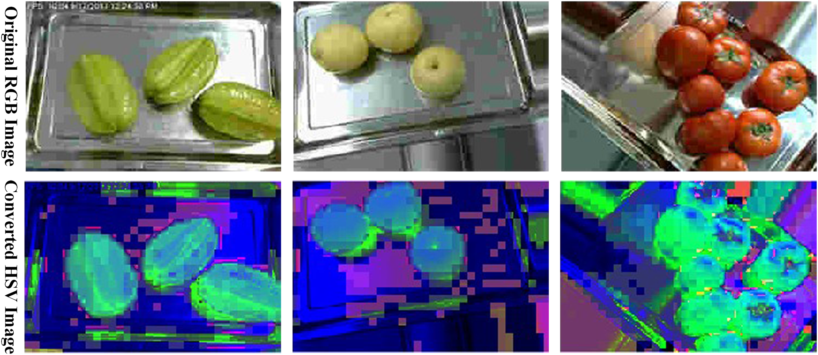
The image processed via the HSV model is shown in Fig. 4. The original RGB image of the star fruit realistically reflects the color and detail of the fruit placed on a metal tray in the actual scene. Each pixel in an RGB image is determined by the values of the three components of red (R), green (G), and blue (B) and constitutes the color world in the image: max=A and min=B are the maximum and minimum values of R, G, and B, respectively. After the original RGB image is converted to the HSV color space, in the HSV image, the star fruit and pear appear blue, because the green component is more prominent in the original RGB image, and in the HSV space, the green is mapped to the range of blue tones. The hue of tomatoes is greener, which may be due to the shift in hue due to the application of different mapping relationships or algorithms in the conversion process, which illustrates the flexibility and diversity of the HSV model in processing images. After thresholding in the HSV color space, the processed image is provided as input to the YOLO v8 model and trained by combining the image RGB color space (Dhal & Das, 2018; Loesdau, Chabrier & Gabillon, 2014) with the HSV color space. This method improves the ability of the model to recognize apples in complex backgrounds as it reduces the interference of background noise and enhances the sensitivity to apple color.
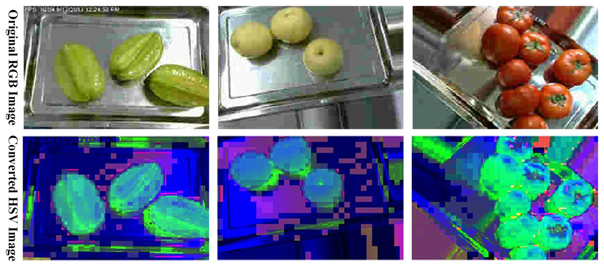
Figure 4: The HSV processing results are compared with the original image.
Color space conversion
Color space conversion (Bi & Cao, 2021) was used to improve model compatibility, optimize feature extraction, and reduce computational complexity among other situations. For apple estimation and recognition in complex backgrounds, the choice of color space conversion converts the image from the default BGR-like color space to the RGB-like color space, ensuring alignment with the standard color space format supported by deep learning models such as YOLO v8 and enhancing interoperability and seamless integration of image data in the recognition process. The RGB color space, with its red-green-blue channels, provides a more intuitive and consistent color representation, which is critical for accurate identification of apples in a variety of environmental conditions and complex backgrounds.
Hiyama et al. (2015) proposed a method called “Band-Limited Double-Step Fresnel (BL-DSF) method” to accelerate the computation of holograms, using color space conversion to accelerate the process of color Computer-Generated Holography (CGH). Chernov, Alander & Bochko (2015) proposed a new fast integer-based algorithm for converting RGB color representations to HSV, which can be a safe alternative to commonly used floating-point implementations. Kamiyama & Taguchi (2021) proposed a method for saturation correction from Hue-Saturation-Intensity (HSI) to RGB, an effective hue and intensity retention saturation correction algorithm. This study prioritizes the conversion of images from the default BGR color space to the RGB color space (Gowri et al., 2022). While BGR and RGB are visually similar, they differ in color coding, especially in image processing. OpenCV and many deep learning frameworks typically use BGR to represent images, and to be more compatible with models such as YOLO v8 and improve color interpretation, there is an urgent need to convert images to the more commonly used RGB color space during the data preprocessing stage. This transformation ensures consistency and accuracy of the color data, helping the model better understand the color information in the image, especially when distinguishing between apples and other objects. Moreover, reducing the correlation between color channels can improve the efficiency and performance of model training.
Labeling dataset
All images were annotated in-house by laboratory members following a unified, standardized protocol to ensure consistency and reproducibility. We employed LabelImg v1.8.1, configured to export annotations in the YOLO format. For each JPEG image, a corresponding TXT file was generated; each line in the TXT file specifies one apple instance by its class identifier and four normalized bounding-box parameters (x-center, y-center, width, height), all scaled to the image dimensions.
The annotation protocol defined two object classes, “ripe_apple” and “unripe_apple,” and established clear rules for bounding-box placement. Annotators were instructed to draw tight boxes around visible fruit edges and to include partially occluded apples if at least 30% of the fruit remained visible. In cases of overlapping fruit, separate annotations were created when the centroids of two fruits were more than 10 pixels apart. This guideline ensured that densely clustered apples were individually captured. Annotation proceeded in a two-stage workflow. First, each lab member independently labeled the full set of 2,500 images. Next, we conducted pairwise cross-validation to identify discrepancies in object counts and box coordinates. Any conflicting annotations were reviewed collectively in consensus meetings until at least 95% inter-annotator agreement was achieved, thereby harmonizing the final label set.
To guarantee annotation fidelity, we executed automated quality checks using a custom Python script. These checks confirmed that no bounding box extended beyond image boundaries, that normalized coordinates lay within the [0, 1] interval, and that every TXT file matched a valid image. Finally, the validated annotations were partitioned into training, validation and test subsets in an 8:1:1 ratio, supporting robust model training and reproducibility.
Apple volume estimation
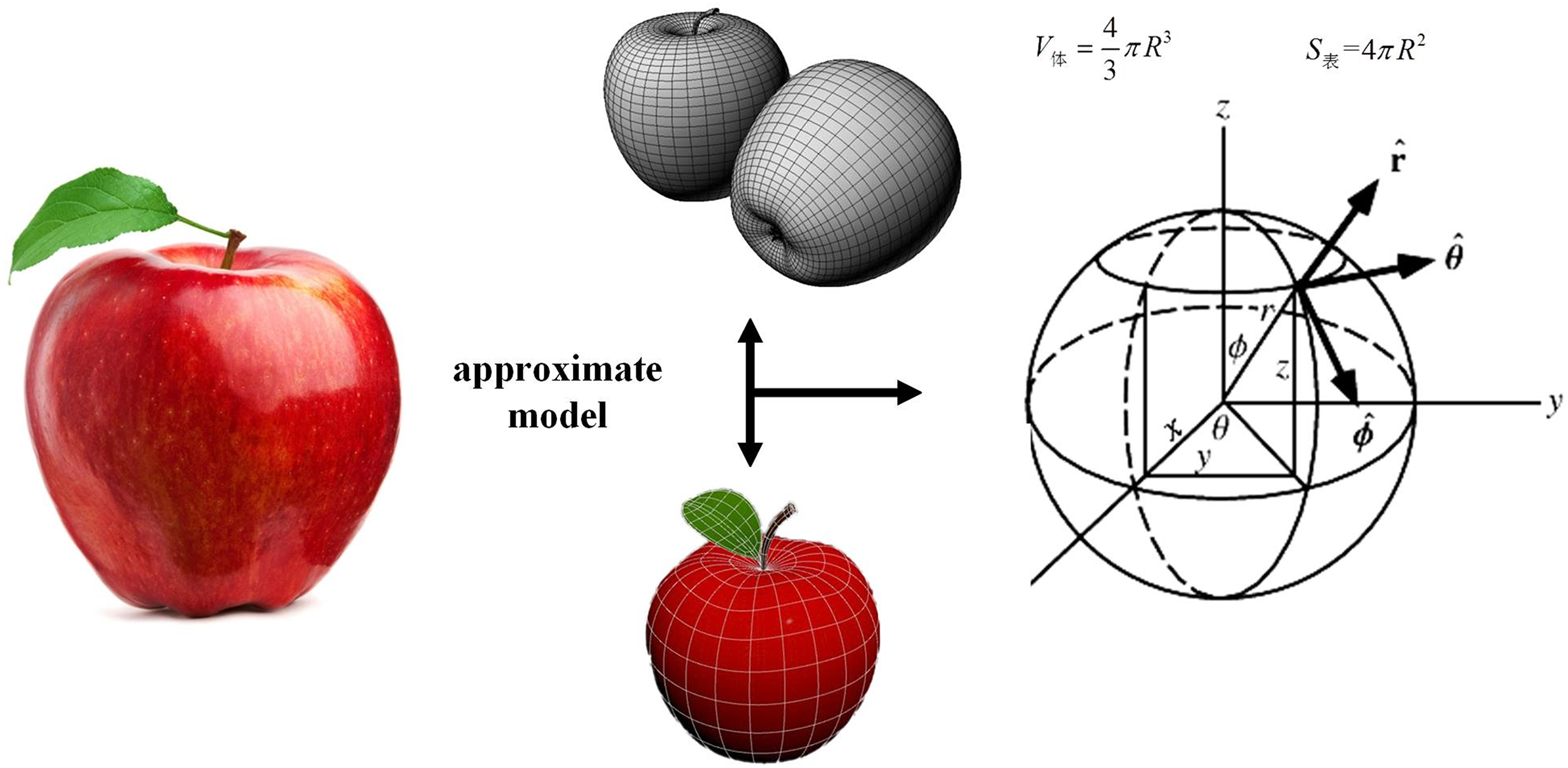
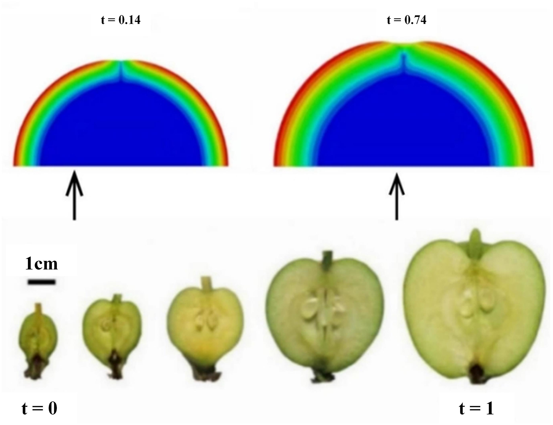
As shown in Fig. 5, the apple is hypothesized to be a sphere, and according to Wang et al. (2016), the final form of apple growth is very close to the positive distribution, so the apple is regarded as a sphere, and the volume of the apple is calculated by measuring the diameter or radius of the apple via the sphere volume formula. Ripe apples are usually fuller and have a larger volume, so by quantifying the change in volume, the level of ripeness of apples can be indirectly assessed. The volume of the sphere can be calculated via the following formula:
(9) where is the sphere’s radius. Since ripe apples typically exhibit larger volumes, quantifying provides an indirect measure of ripeness.
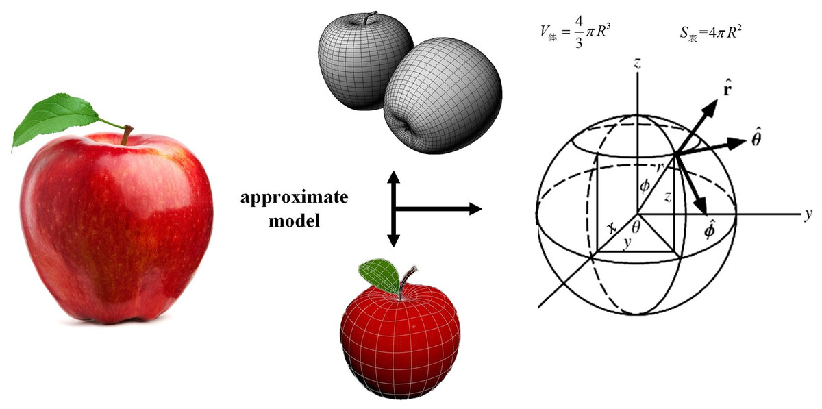
Figure 5: Three-dimensional model of an apple.
Rather than inferring directly from a single two-dimensional bounding box, we first reconstruct a three-dimensional point cloud using multiview RGB images from the YOLO v8 detection pipeline and corresponding camera calibration data. Fitting a sphere to this point cloud yields an accurate estimate of that incorporates true depth information and overcomes the limitations of purely 2D approaches in complex orchard scenes.
In practical implementation, however, YOLO v8 provides only a set of 2D bounding boxes for each detected apple. To bridge the 2D and 3D domains, we derive an initial estimate of from the average width of multiple overlapping bounding boxes within a single view. This estimate then serves as a starting value for our sphere-fitting algorithm, producing a refined radius that closely matches the true apple dimensions.
(10)
In accordance with Zhao, Pang & Zhang (2024), the relationship between the maturity judgment and the volume of apples was understood. The radius deduced from the obtained area was brought into the hypothetical apple sphere model to obtain the volume, and then the maturity distribution was determined by judgment. Different thresholds were set according to the volume by the maturity judgment, and a small number of samples were manually selected for the same model calculation and finally compared with the maturity frequency map to confirm the feasibility and accuracy of the model. The model was trained to identify and classify the images of the apple dataset. This method can provide a quick and intuitive way for growers or market practitioners to determine if the apple is at the optimal time to pick.
YOLO v8 model
As the latest version of the YOLO series (Jiang et al., 2022), YOLO v8 (Talaat & ZainEldin, 2023) has improved speed and accuracy and is particularly suitable for handling recognition tasks in complex backgrounds, as shown in Fig. 6. Compared with the traditional two-stage recognition method, YOLO v8 has faster detection speed and higher efficiency.
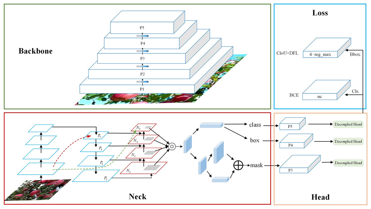
Figure 6: YOLO v8 structure diagram.
The backbone network efficiently extracts features from the input data. The head network classifies and localizes targets on the basis of backbone features. The neck network sits in between and facilitates feature fusion and reinforcement to ensure effective information delivery. During training, Bbox loss quantifies and reduces bounding box prediction bias, and Cls loss evaluates category prediction accuracy and optimizes it. The two work together to improve model performance.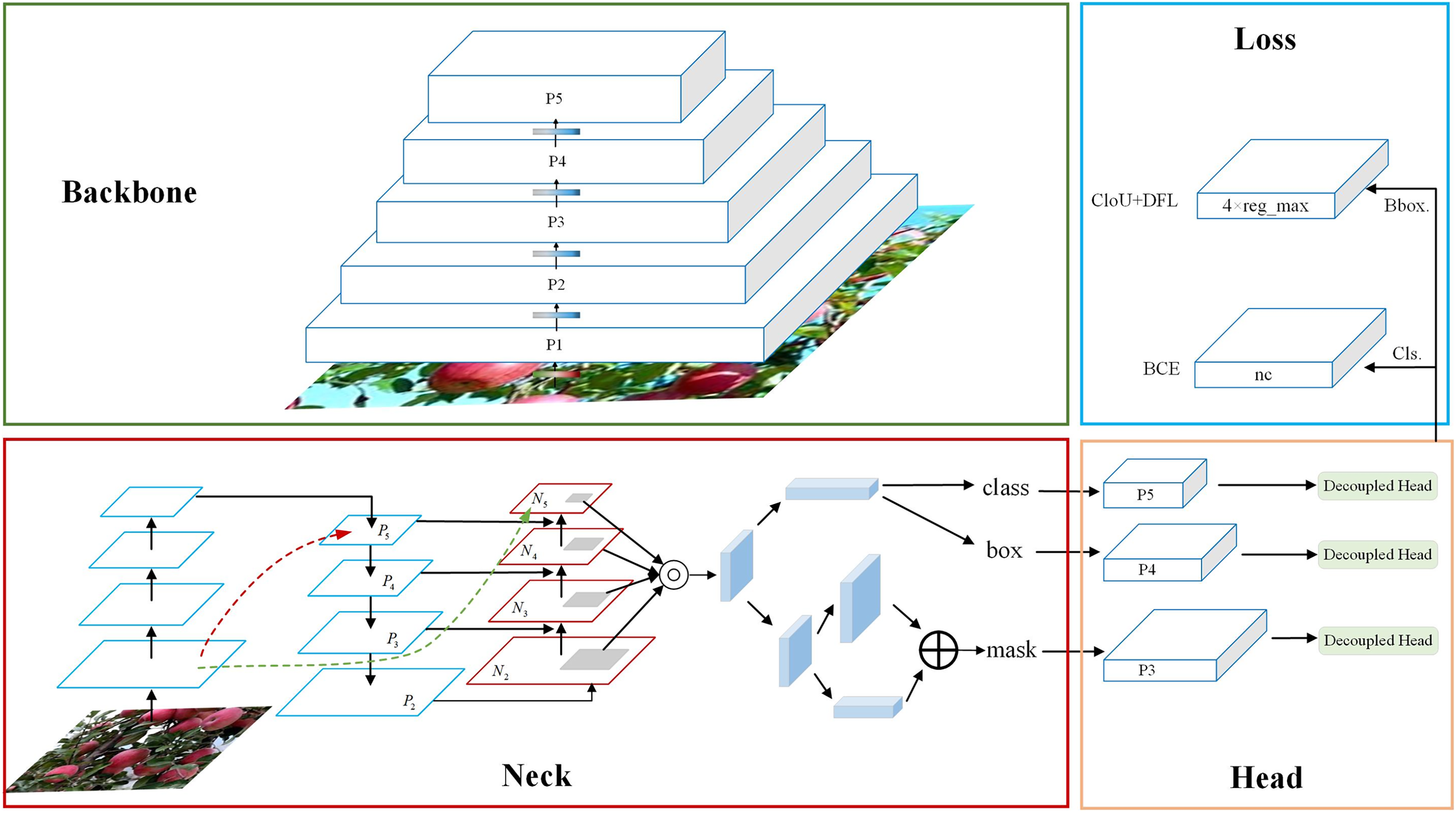
In this work, YOLO v8 was selected as the main deep learning model because of its excellent performance and wide application in recognition tasks. YOLO v8 uses a series of advanced technologies, including multi-scale feature fusion, multi-scale prediction, and the introduction of attention mechanisms, to improve detection performance and accuracy (Kashyap, 2024; Razaghi et al., 2024). Its recognition model can quickly and accurately identify multiple targets in the image, use a single neural network to complete target detection and position positioning in a single processing step, and use feature maps of different scales to detect targets of various sizes, which improves the model’s ability to identify targets of different sizes, and can simultaneously predict target categories and accurately regress positions. Moreover, YOLO v8 under the maximum model is selected to increase the accuracy of the results so that the model is more accurate or more efficient in the recognition task. Images from the default BGR color space are converted to the RGB color space to improve model compatibility and accuracy. Color space conversion helps the model better understand the color information in the image, especially to accurately identify apples in complex backgrounds. Overall, the apple estimation and recognition system based on the YOLO v8 model has significant performance advantages in complex backgrounds and provides important support and guidance for the development of apple recognition technology by combining advanced deep learning technology and effective data preprocessing methods.
Experiment and analysis
Evaluation metrics
To evaluate the effectiveness of the YOLO v8 model, a series of accurate evaluation indicators were used to measure its accuracy and efficiency to evaluate the effectiveness of the model. These metrics include accuracy, precision, recall, F1-score, AP, P-R curve, Receiver Operating Characteristic (ROC), Area Under the Curve (AUC), and other indicators. For the following formula, T (true) represents the recognition target, F (false) represents the unrecognition target, P (positives) represents the correct recognition, N (negatives) represents the recognition failure, TP represents the recognition target, which is successfully identified as the recognition target, FP represents the non-recognition target, misidentified as the recognition target, TN represents the recognition target, incorrectly identified as the unclassified target, FN represents the non-classified target, and incorrectly identified as the non-classified target.
ACC (Accuracy): this reflects the ability of the classifier or model to judge the overall sample correctly, that is, the ability to correctly classify positive (positive) samples and negative (negative) samples correctly. The model’s ability to judge the overall sample correctly is reflected, and the higher the value is, the better. However, when the sample is not balanced, the accuracy cannot evaluate the model performance well.
(11)
Precision: this reflects the ability of the classifier or model to correctly predict the accuracy of positive samples, that is, how many of the predicted positive samples are real positive samples, and the higher the value is, the better.
(12)
Recall: the proportion of samples that are positive that are correctly predicted by the model to be positive. This reflects the model’s ability to correctly predict the purity of positive samples, with higher values being better.
(13)
F1-score: the harmonic average of precision and recall, which is used to comprehensively evaluate the precision and recall of the model.
(14)
P-R graph: with recall as the horizontal axis and precision as the vertical axis, the corresponding recall values of each point in the Precision [0, 1] range are connected to form a broken line, which is used to visually show the performance of the model under different precisions and recalls. As the recall value increases, the precision value gradually decreases, eventually fluctuating up and down around a certain value.
Average Precision (AP) measures the area under the precision–recall curve and thus reflects the trade-off between precision (the proportion of true positives among detected instances) and recall (the proportion of true positives detected among all ground-truth instances). In our implementation, we compute AP by sampling the precision at 101 equally spaced recall levels and integrating over the recall axis, following the Common Objects in Context (COCO) evaluation protocol. A higher AP indicates that the model maintains both high precision and high recall across varying confidence thresholds, providing a comprehensive assessment of detection performance.
The training process
In this study, the recognition head of the network was originally configured for 80 classes (the number of categories in the COCO dataset); however, because our task focuses exclusively on apple detection, it was reduced to a single class. The remaining training hyperparameters (Table 2) included a per-Graphics Processing Unit (GPU) batch size of 16, eight data-loading workers, 500 epochs, and an input image resolution of 640 × 640 pixels. The weight assigned to the recognition loss was 0.5, and the bounding-box regression loss weight was 7.5. Under these conditions, together with the model’s training scripts and preprocessing pipeline, the system accurately detected and enumerated apples in each image, presenting the results in a clear visual format. Additionally, an HSV-based module was employed to assess the ripeness category of each detected apple, thereby enabling detailed analysis and interpretation of fruit maturity.
| Number | Parameter | Setting |
|---|---|---|
| 1 | Per-GPU batch size | 16 |
| 2 | Data-loading workers | 8 |
| 3 | Maximum epochs | 500 |
| 4 | Input resolution | 640 × 640 |
| 5 | Recognition loss weight | 0.5 |
| 6 | Bounding-box regression loss weight | 7.5 |
In terms of hardware, to train deep learning models with the dense architecture of YOLO v8, this article uses a Dell Tower T440 server and an RTX 4090 GPU, whose parallel processing capabilities significantly accelerate the speed of model training and inference. Moreover, the Solid State Drive high-speed storage solution is used to improve the fast access speed of data during training and minimize the impact of I/O bottlenecks. With the help of a high-quality software environment and powerful hardware settings, the apple estimation and recognition task was successfully trained in complex backgrounds, and a model with enhanced accuracy and performance was obtained. The synergy between software tools and hardware resources plays a key role in the deep learning-based apple recognition task to achieve the best results.
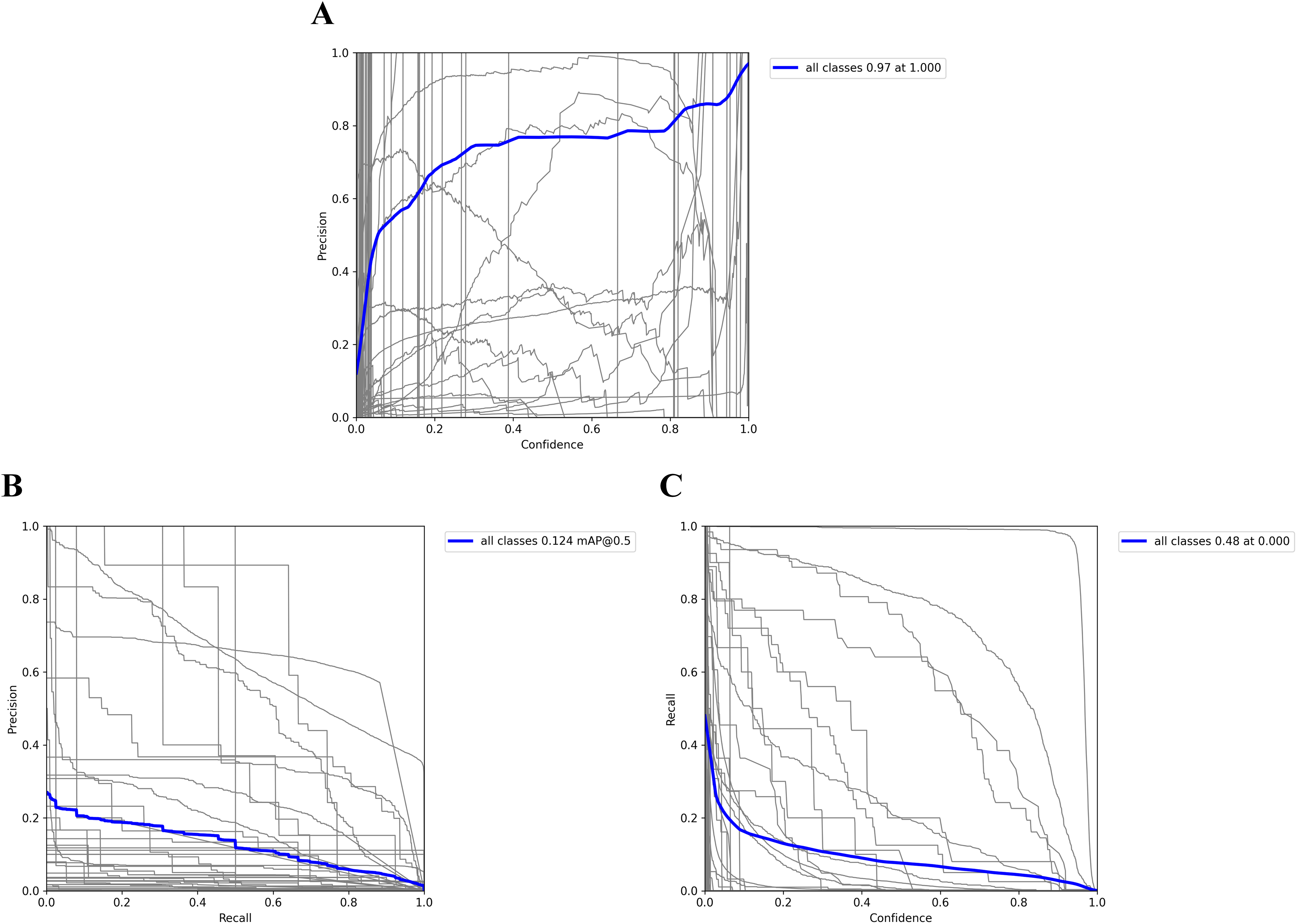
As shown in Fig. 7, the steeper the upwards trend of the P-R curve is, the higher the accuracy of the model at lower thresholds. As shown in Fig. 7A, when the PR curve trends upwards, the accuracy of the model improves while maintaining high recall. Figure 7B illustrates the trade-off between the accuracy and recall of the model at different thresholds. The relationships between precision and confidence and recall are evident in Fig. 7C, specifically, because the P-curve increases sharply in the lower threshold range, the model is fully accurate in classifying the sample as positive, i.e., there are few mispositives. Moreover, the PR curve gradually approaches one with the change in P, which can indicate that the recognition of the model has good performance and a good recognition effect.
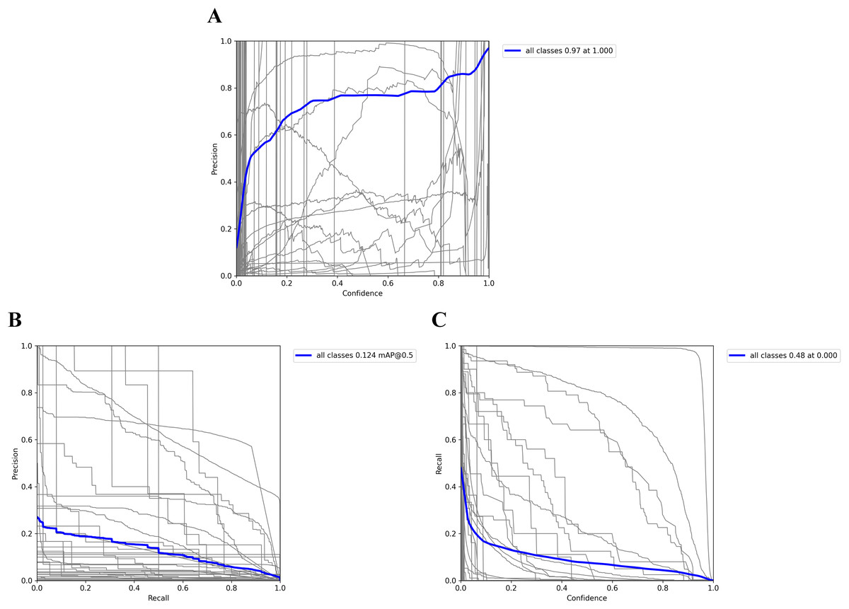
Figure 7: (A) P_curve, (B) PR_curve and (C) R_curve for the test set.
Phenotypic measurement of apple in complex scenes
The number of apple
To solve the challenge of estimating the number of apples, this article uses the input image to go through a preprocessing stage, including grayscale conversion, Gaussian filtering for noise reduction, edge smoothing through morphological operations, and edge detection via Canny and Sobel operators to enhance feature extraction and depiction. The processed images were fed into the YOLO v8 model, which performed well because of its high efficiency and accuracy in recognition tasks. The model analyses the image data and generates a bounding box around the detected apples. After recognition, a counting algorithm is implemented to determine the total number of apples on the basis of the determined bounding box, and the model is used to retrieve the number of apples in each picture and draw a distribution map of the number of apples in each picture in the dataset. Finally, the feasibility of the YOLO v8 detection model was determined.
After preprocessing, the data are brought into the detection model, and the color features, shape features, and cultural and scientific features of the image are extracted through YOLO v8. The apple is accurately identified, the apple on the picture is feature captured, and Figs. 8A–8D are obtained, which is based on the mature apple image set provided in the dataset. The YOLO v8 recognition model is used to lock the apple to extract the color features, texture features, and shape features of the image, and the search mechanism is used for preliminary learning. Then the results obtained by the sample are manually detected. If it is determined that it is feasible, the resulting apple-locking algorithm is applied to the entire population to obtain the number of apples in each of the 200 images in the file.
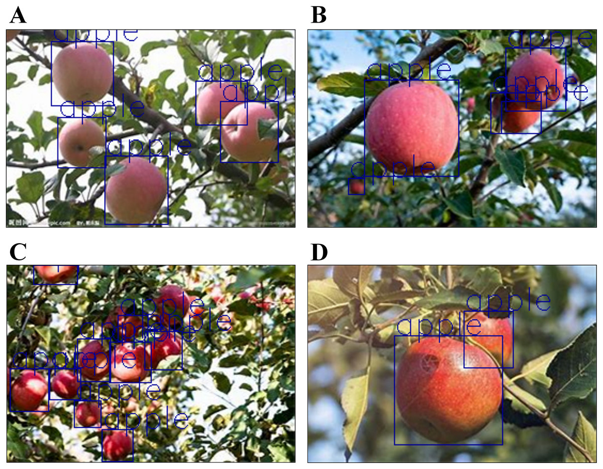
Figure 8: Recognition results of the coordinate position of the apple via the YOLO v8 network.
(A) Backlighting, (B) different fruit sizes, (C) exposure and leaf shading, and (D) fruit shading.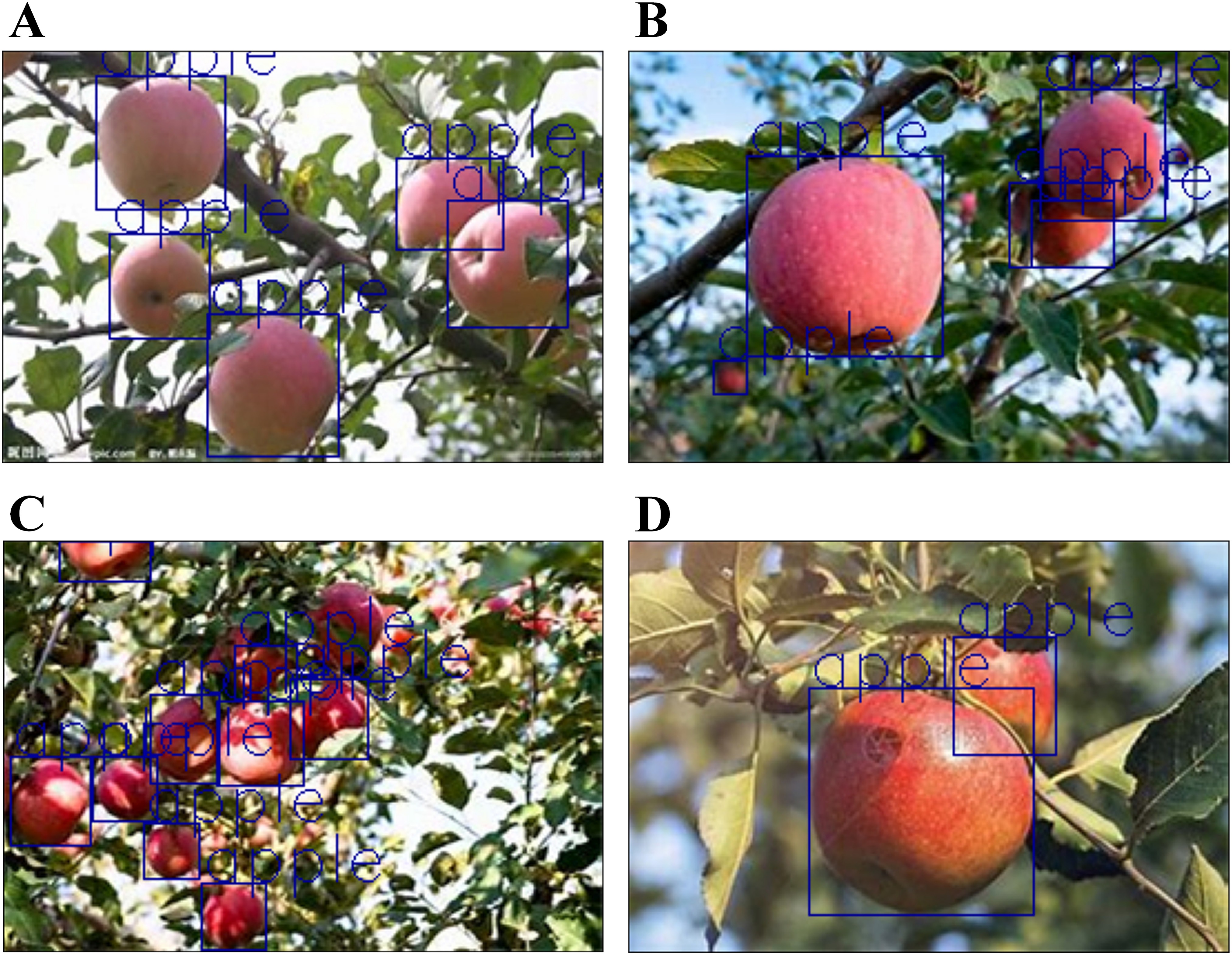
The YOLO v8 model was used to detect and analyse 200 preprocessed images one by one, and the number of apples in each image was obtained. The model uses its efficient detection speed and precise recognition ability to locate the apple quickly and accurately in each image. After careful analysis of the model, the number of apples in each image is clearly visible. Due to the large amount of data, some randomly selected test results are shown in Table 3 (see Appendix 4(1) for details.). As seen from the data in the table, there is a major difference in the number of apples in different images, which may be related to factors such as the shooting angle of the image, lighting conditions, and size and density of the apples. However, regardless of its number, the YOLO v8 model can identify and count accurately, providing reliable data support.
| Picture serial number | Number of apples |
|---|---|
| 4 | 11 |
| 5 | 9 |
| 7 | 22 |
| 12 | 11 |
| 14 | 10 |
| 24 | 17 |
| 33 | 10 |
| 39 | 14 |
| 44 | 11 |
| 57 | 8 |
| 67 | 11 |
| 75 | 10 |
| 88 | 10 |
| 110 | 2 |
| 126 | 11 |
| 147 | 17 |
| 151 | 2 |
| 164 | 10 |
| 188 | 4 |
| 200 | 14 |
The positions of the apple
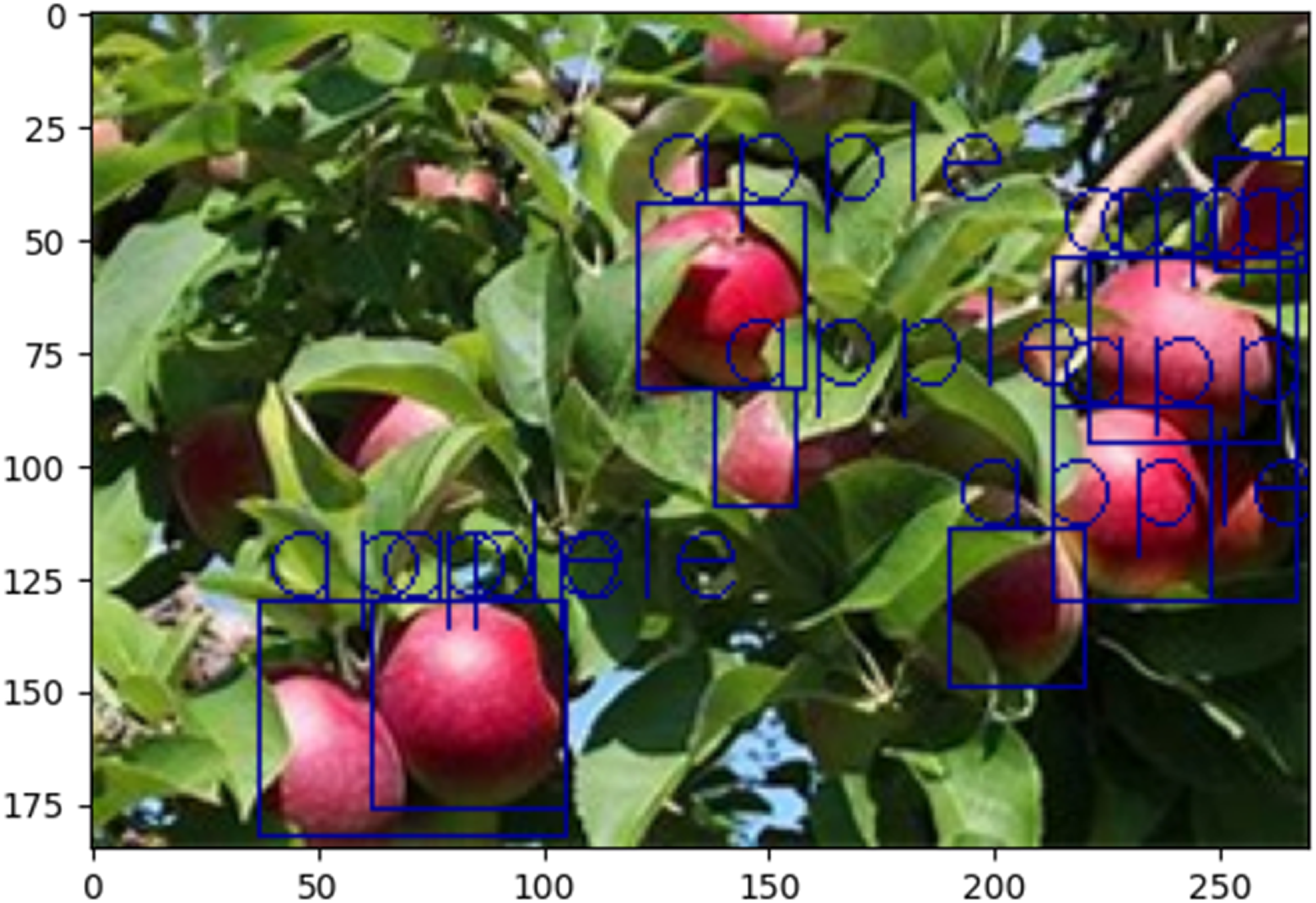
In the context of apple estimation in a complex context via the YOLO v8 model, it is critical to determine the precise location of the detected apple. The YOLO v8 recognition model was first trained with the image set of apples. The analytical output was used to find the bounding box related to the apple, and the center of the bounding box was used to represent the position of the apple to draw a two-dimensional scatter map of the geometric position of the apple in 200 images. Using the YOLO v8 recognition model, the model is trained on an annotated image dataset containing apples on the tree, and the model learns to detect apples in the image and outputs the corresponding bounding boxes and category labels. The trained model is subsequently used to infer the new image, and the model returns the bounding box and related information of the detected object. After that, the output is parsed, each bounding box is output with an associated category label and confidence score, and the bounding box related to the apple is found. The position coordinates are obtained, the bounding box containing the apple is identified, as shown in Fig. 9. The final apple position information is extracted from the coordinates of the bounding box, which are the upper left point and the lower right point of the box, and four values are obtained, which are the coordinates of the upper left and lower right points. The values of two x are averaged, and the values of two y are averaged to obtain the center point of the box.
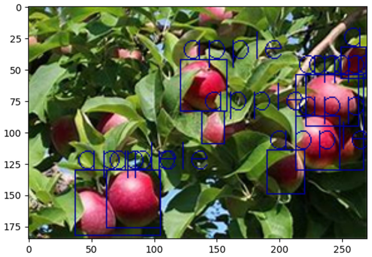
Figure 9: The recognition results of YOLO v8 under close-exposure and closed-conditions.
Let the coordinates of the upper left corner of the bounding box be , the coordinates of the lower right corner of the bounding box be , and the mathematical expressions of the horizontal and vertical coordinates of the center point of the bounding box are:
(15)
The center coordinates of the bounding box indicate the approximate position of the apple in the image, and the position information of the apple in each image is stored in Appendix 4(2). The model extracts the center coordinates of apples from 200 images and maps them uniformly into the same coordinate system. As shown in Table 4, given the large amount of data, some of the location coordinates were randomly extracted for the analysis (see Appendix 4(1) for details).
| Number | X | Y |
|---|---|---|
| 16 | 158.5 | 86 |
| 79 | 155.5 | 78.5 |
| 139 | 80 | 55.5 |
| 145 | 262.5 | 153 |
| 361 | 10 | 83 |
| 438 | 87.5 | 98 |
| 598 | 27.5 | 129 |
| 599 | 68.5 | 85 |
| 700 | 149.5 | 86 |
| 701 | 263.5 | 164.5 |
| 813 | 46 | 103.5 |
| 830 | 82.5 | 114 |
| 913 | 156.5 | 156.5 |
| 985 | 197 | 35 |
| 1,022 | 135 | 118.5 |
Maturity state of apple
To solve the ripening state of apples, the HSV model was used to judge and analyse the apple ripeness categories in the image for each apple, and the output categories were divided into four categories: ripe, unripe, semi-immature, and extremely immature. According to the judgment of the HSV model, the following scatter plots and histograms are drawn, as shown in Fig. 10 below. We imported the matplotlib.pyplot library and created an alias plt for it. The plt.scatter function is used to draw the graph title and axis labels are added, and finally, plt.show ( ) is used to display the graph.
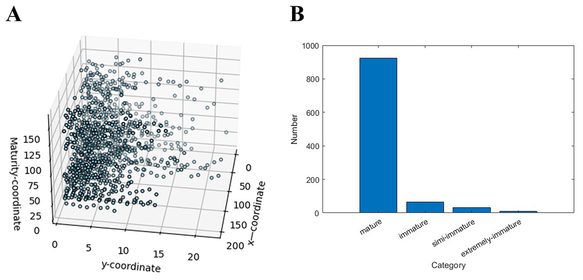
Figure 10: Distribution of apple ripeness.
(A) Visualization of apple ripeness, and (B) concentrated display of apple ripening distribution in the dataset.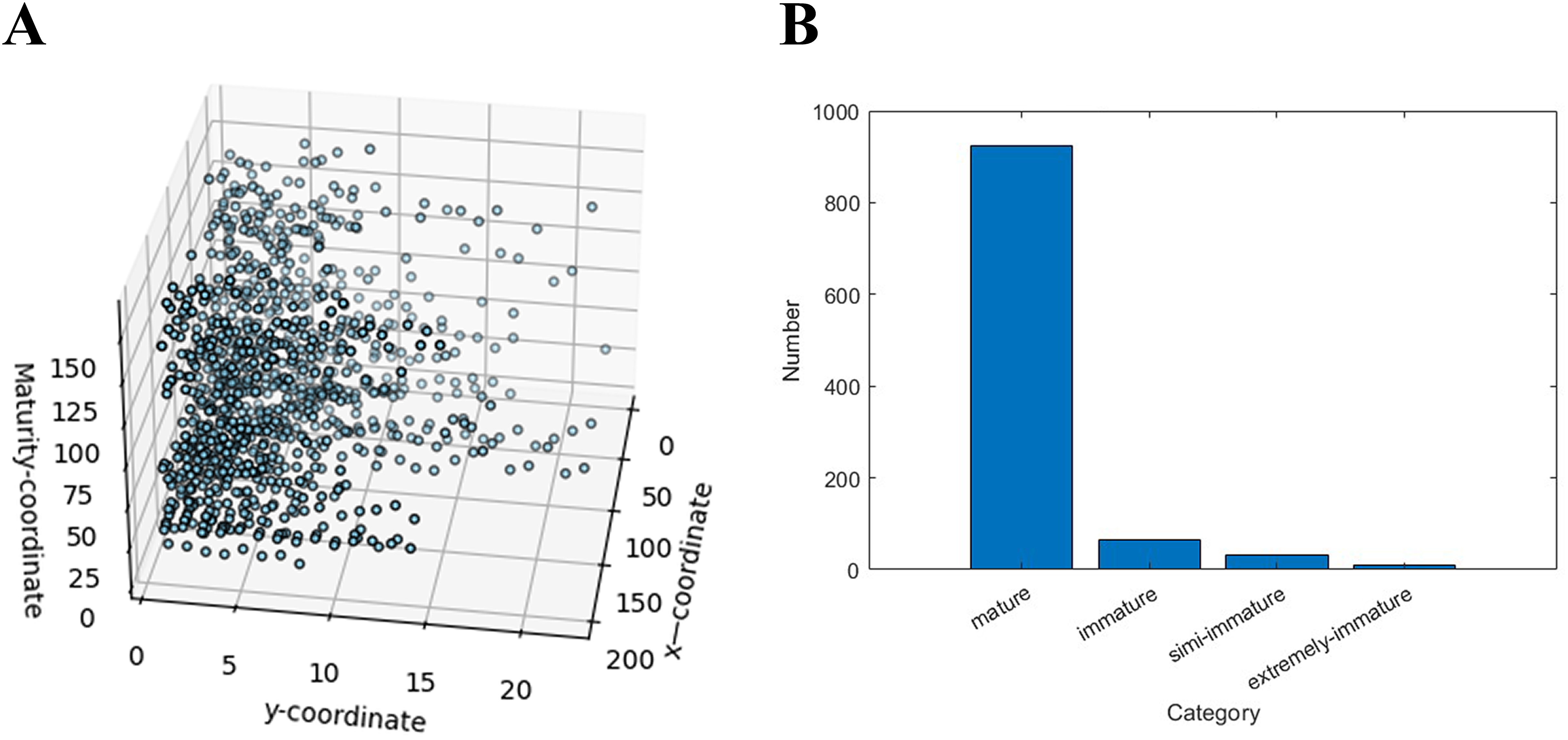
In Fig. 10A, and are the coordinates of the image, and is the maturity level, and the maturity of the product can be analyzed on basis of the distribution and trend of the data points. The distribution of the ripeness of all apples in Appendix 4(3) shows a clear upwards trend in the value of as the number of or increases. This shows that with increasing characteristics of the apples, their ripeness also gradually increases. In the graph, the concentration of data points also reflects the maturity of the apples. When the data points are more concentrated, the ripeness of the apple is greater, and when the data points are more scattered, the maturity of the apple is lower. Sometimes there are outliers, i.e., those that deviate from the main distribution trend. This may be due to an error in the data collection or processing process, or it may be due to a specific problem or defect in the apple. The ripeness of the apples was assessed by looking at the shape and distribution shown in Fig. 10B, with ripeness being the majority.
Weight of apple
Calculating the weight of apples plays a key role in accurately assessing their size and quantity. This step involves analyzing the size and pixel values of the detected apples to derive their respective qualities. The YOLO v8 recognition model was used to detect the apple radius, the apple mass was obtained via the mass formula, and the apple mass distribution map was drawn. YOLO v8 is a recognition checkpoint trained on a COCO detection dataset with an image resolution of 640, an instance segmentation checkpoint trained on a COCO segmentation dataset with an image resolution of 640, and an image recognition model pre-trained on an ImageNet dataset with an image resolution of 224.
In YOLO v8, some changes have been made to the model structure. Compared with YOLO v5, the backbone and neck of YOLO v8 have changed. Specifically, the kernel of the first convolutional layer changed from 6 × 6 to 3 × 3. All C3 modules are replaced with C2f, a structure with more hop connections and additional split operations. The two convolutional layers in the neck module were eliminated. The number of C2f blocks in backbone has been changed from 3-6-9-3 to 3-6-6-3. When there are multiple rectangular boxes in a graph, we need to sum and average each box. First, we define a function called detect_colorinom, which converts the read image from the BGR color space to the HSV color space, calculates the hue histogram of the selected area and calculates the average of the hue channels. It accepts a range of parameters, including the image number, number of boxes, number of bounding boxes, color tone, image path, and the , , , and coordinates of the region.
According to the analysis of the apple area data in Appendix 4(4), the distribution of the apple area was relatively uniform, with a certain degree of fluctuation. After synthesizing the area data of each apple, it was found that it conformed to the characteristics of a normal distribution. This confirms the feasibility of the model, allowing the quality equation to be applied based on it:
(16)
According to the literature, it has been concluded that the mass and area of apples generally follow the same normal distribution. The apple weight data obtained in this study were expected to conform to a normal distribution. Figure 11 (Chakrabarti et al., 2021) shows that the frequency distribution of the original area exhibits an approximate normal distribution, which was consistent with the experimental data. Based on the details of the apple weight data in Appendix 4(4), the analysis confirmed the validity of the model. This indicates that all data can be exported confidently.
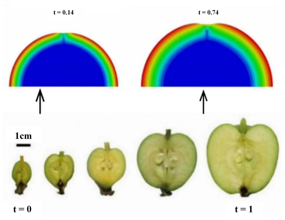
Figure 11: Frequency distribution of the original area of the apples.
Apple recognition in complex scenes
To assess the effectiveness of the YOLO v8 model for apple estimation and recognition, we compared its performance against widely used models, including VGG (Pandiyaraju et al., 2025), ResNet (Wu et al., 2025), and MobileNet (Wijayanto, Swanjaya & Wulanningrum, 2024). All models were evaluated on the same apple dataset under identical experimental conditions. The results, presented in Table 5 highlight the comparative performance and detection capabilities of each model in this task.
| Network model | Precision (%) | Recall (%) | mAP (%) | F1 (%) | Test time (s) | Mean confidence (95% CI) |
|---|---|---|---|---|---|---|
| VGG | 90.50 | 95.37 | 94.86 | 92.87 | 0.02 | 83.7 ± 6.3% |
| ResNet | 85 | 76 | 87 | 80.25 | 0.13 | 67.7 ± 6.2% |
| MobileNet | 77.78 | 86.48 | 75.67 | 81.92 | 0.02 | 81.2 ± 6.0% |
| YOLO v8 | 93.1 | 93.8 | 95 | 93.45 | 0.19 | 96.4 ± 1.2% |
This study evaluates the performance of apple localization and detection models in complex orchard environments using the YOLO v8 framework. Mean average precision (mAP) and F1-score are the primary evaluation metrics. The YOLO v8 model achieves an mAP of 95.0%, an F1-score of 93.45% and mean confidence of 96.4% (95% confidence interval (CI) [95.2–97.6%]), demonstrating high detection accuracy with minimal false positives and false negatives.
The experimental design simulates realistic orchard conditions, including lighting variation, fruit occlusion and complex backgrounds. Each model was evaluated on the same apple dataset and compared across key metrics. YOLO v8 consistently outperforms VGG, ResNet and MobileNet in precision, recall, mAP and F1-score. Specifically, YOLO v8’s precision of 93.10% and mAP of 95.00% represent improvements of approximately 2.6% and 1.5%, respectively, over the next-best model. Although VGG attains a marginally higher mAP than some baselines, YOLO v8’s superior F1-score (93.45% vs 92.87%) reflects a more balanced trade-off between precision and recall. Moreover, we computed the mean predicted confidence and its 95% confidence interval (CI) over all detections to quantify detection stability: YOLO v8 attains a mean confidence of 96.4% (95% CI [95.2–97.6%]), markedly higher and more consistent than the competing models. These confidence intervals demonstrate YOLO v8’s ability to make highly reliable predictions even under challenging lighting, occlusion, and background clutter.
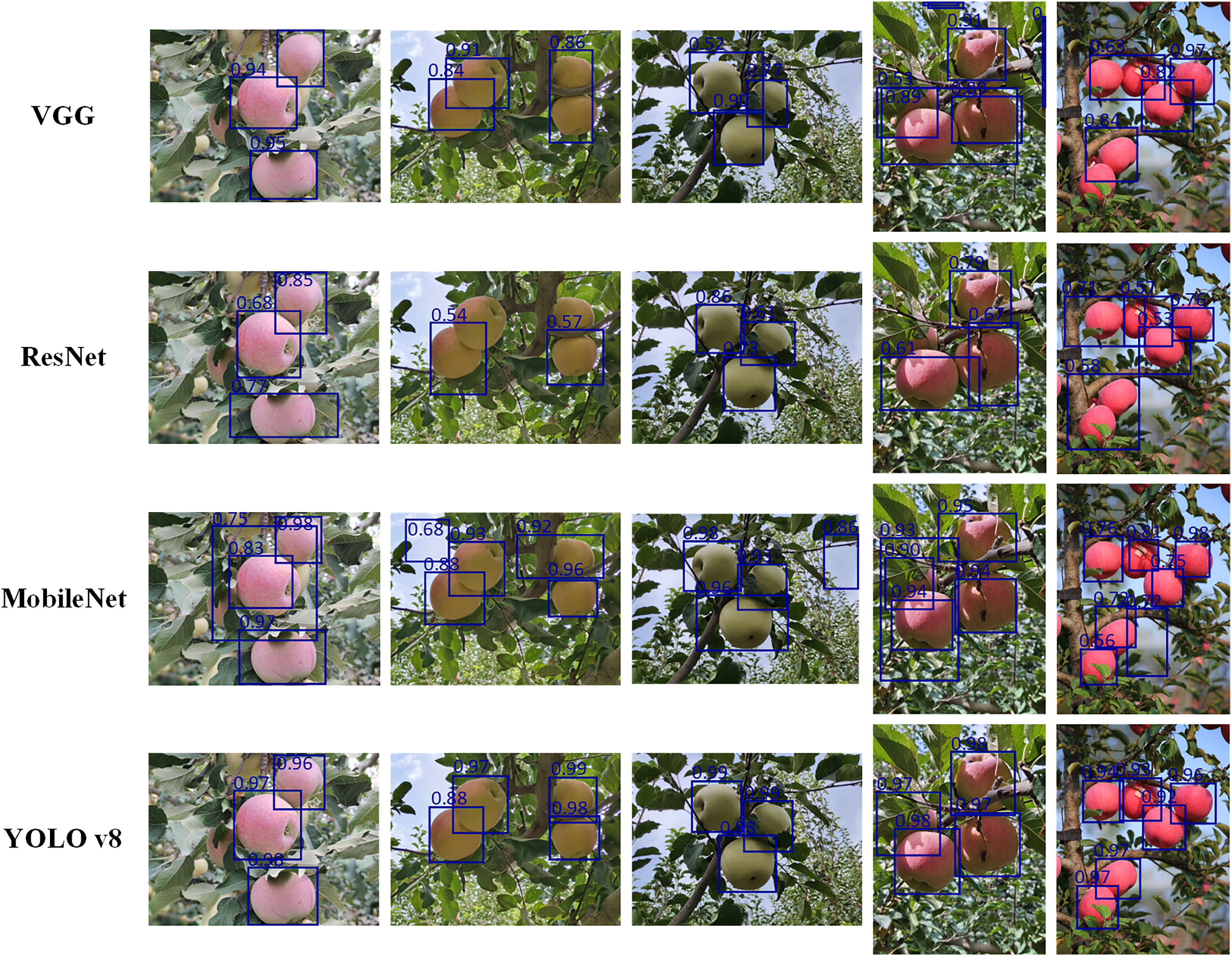
Figure 12 presents representative detection visualizations for each model, highlighting the superior balance achieved by YOLO v8 between high confidence scores and precise localization. In our experiments, VGG produced comparatively wide bounding boxes that frequently overlapped with surrounding foliage in complex scenes, yielding only moderate confidence scores ranging from 0.63 to 0.90 and struggling to detect small or occluded apples. ResNet delivered tighter boxes but suffered from false positives in clusters of fruit, with confidence scores fluctuating broadly between 0.57 and 0.96. MobileNet achieved accurate localization and confidence levels of at least 0.75 when apples were well separated. However, its performance degraded under heavy occlusion or overlap, occasionally producing duplicate or fragmented boxes. In contrast, YOLO v8 consistently generated highly precise, tightly fitted boxes across all test images and maintained uniformly high confidence levels between 0.92 and 0.99, with negligible false positives or missed detections, demonstrating the best overall detection performance.
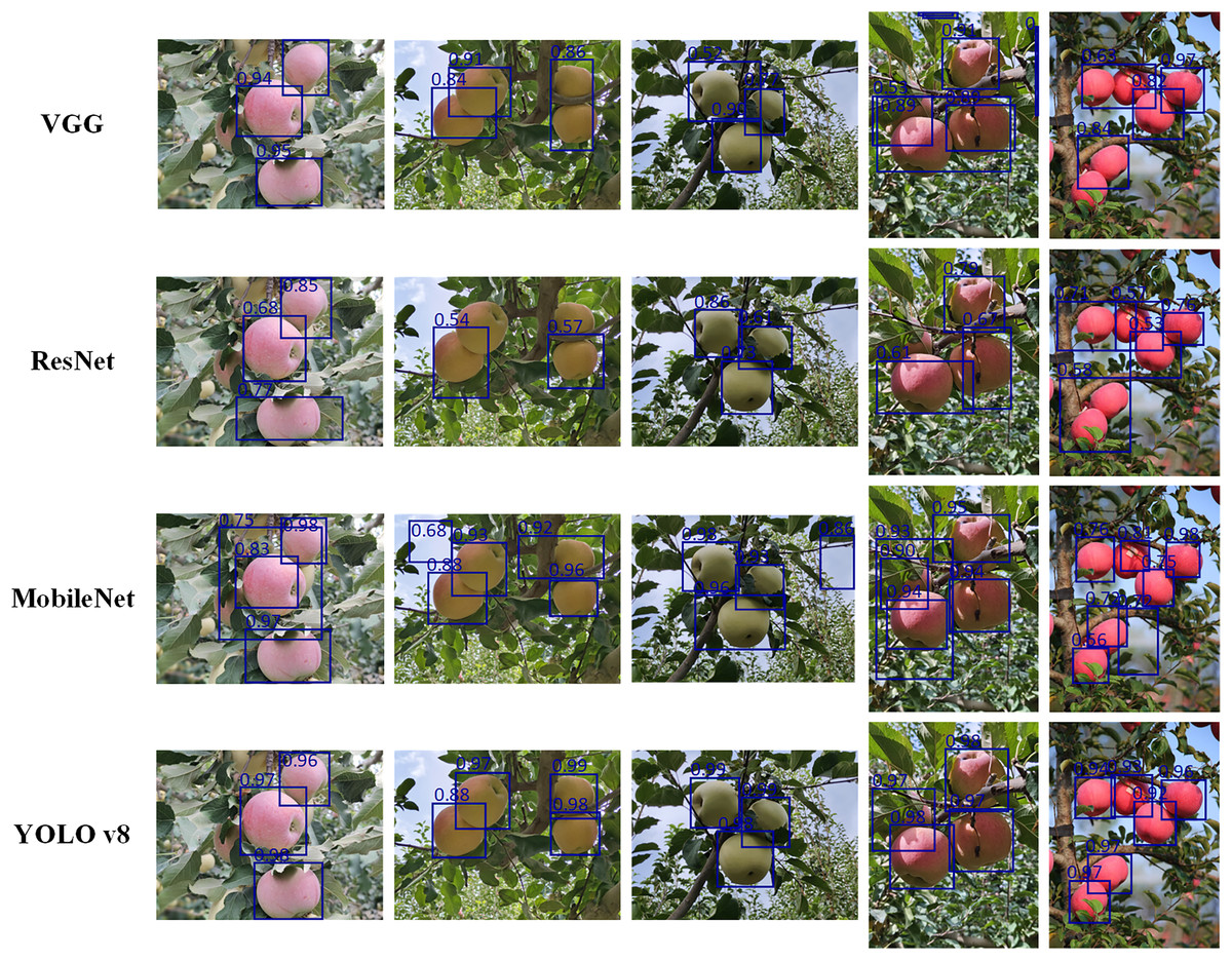
Figure 12: Apple detection visualizations by VGG, ResNet, MobileNet, and YOLO v8 in complex orchard environments.
Importantly, YOLO v8 processes each image end to end, including both localization and classification, in just 0.19 s while maintaining a mean detection confidence of 96.4% (95% CI [95.2–97.6%]). By comparison, VGG and MobileNetV2 require 0.02 s for feature extraction alone, and ResNet requires 0.13 s. These results demonstrate that, despite performing full object detection, YOLO v8 preserves real-time inference capability. Furthermore, its streamlined architecture reduces computational load, parameter count, and memory consumption, making it particularly well suited for deployment on embedded devices in autonomous harvesting robots.
Discussion
Recognition of other fruits based on YOLO v8
The purpose of this research is to evaluate and recognize the number of apples in a complex background via a target detection model that is based on YOLO v8. To ensure the model’s generalizability ability and accuracy, with the potential value of generalization to other fruit species, Fig. 13 demonstrates the model’s performance in handling the variable fruit detection task, which includes a variety of similarly shaped and colored fruits with multiple detection experiments conducted at different angles, lighting, and background interference. The results of the training samples indicate that most of the fruits are correctly detected and localized, effectively avoiding the problem of other fruits being misidentified as apples. The training dataset is expanded to cover a wide range of fruit varieties, the model parameters are tuned to accommodate different shapes and colors, and the algorithm is fine-tuned to improve the specificity and accuracy of the fruit recognition task. In the field of crop research, current attention is focused on oleaginous fruits, wheat, corn, apples and strawberries. While most studies have focused on a single species, this study is based on the identification of five fruits under different light and angle conditions, with a special focus on the location and ripeness of apples.
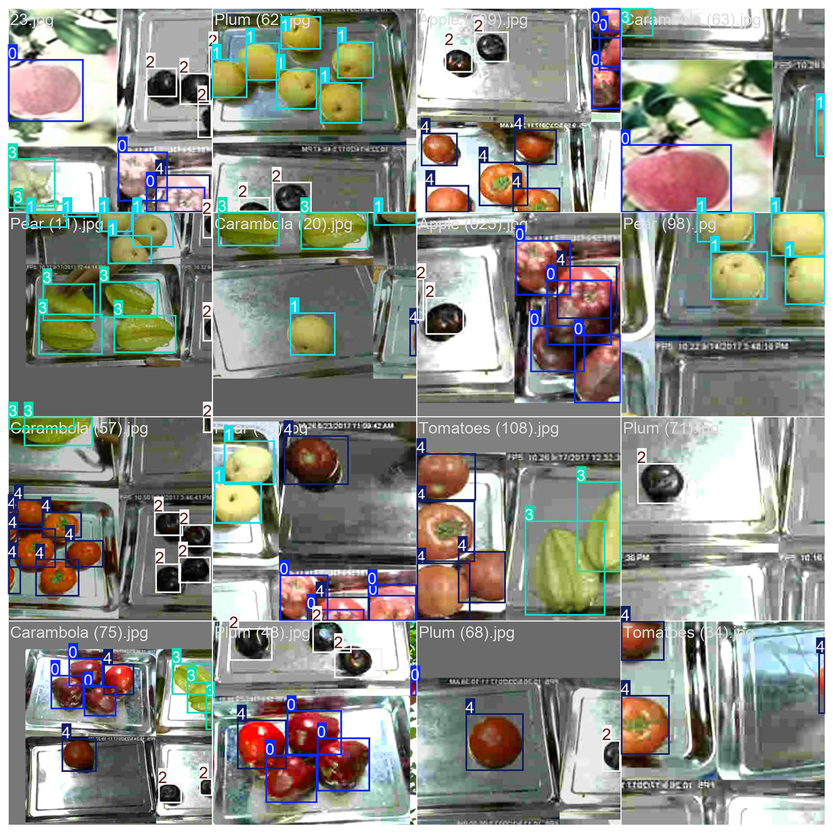
Figure 13: Category recognition image of an apple.
Recognition and detection of two fruits under different lighting and five fruits under the same lighting. The image also contains the challenge of recognizing the lack of integrity due to the occlusion of some fruit.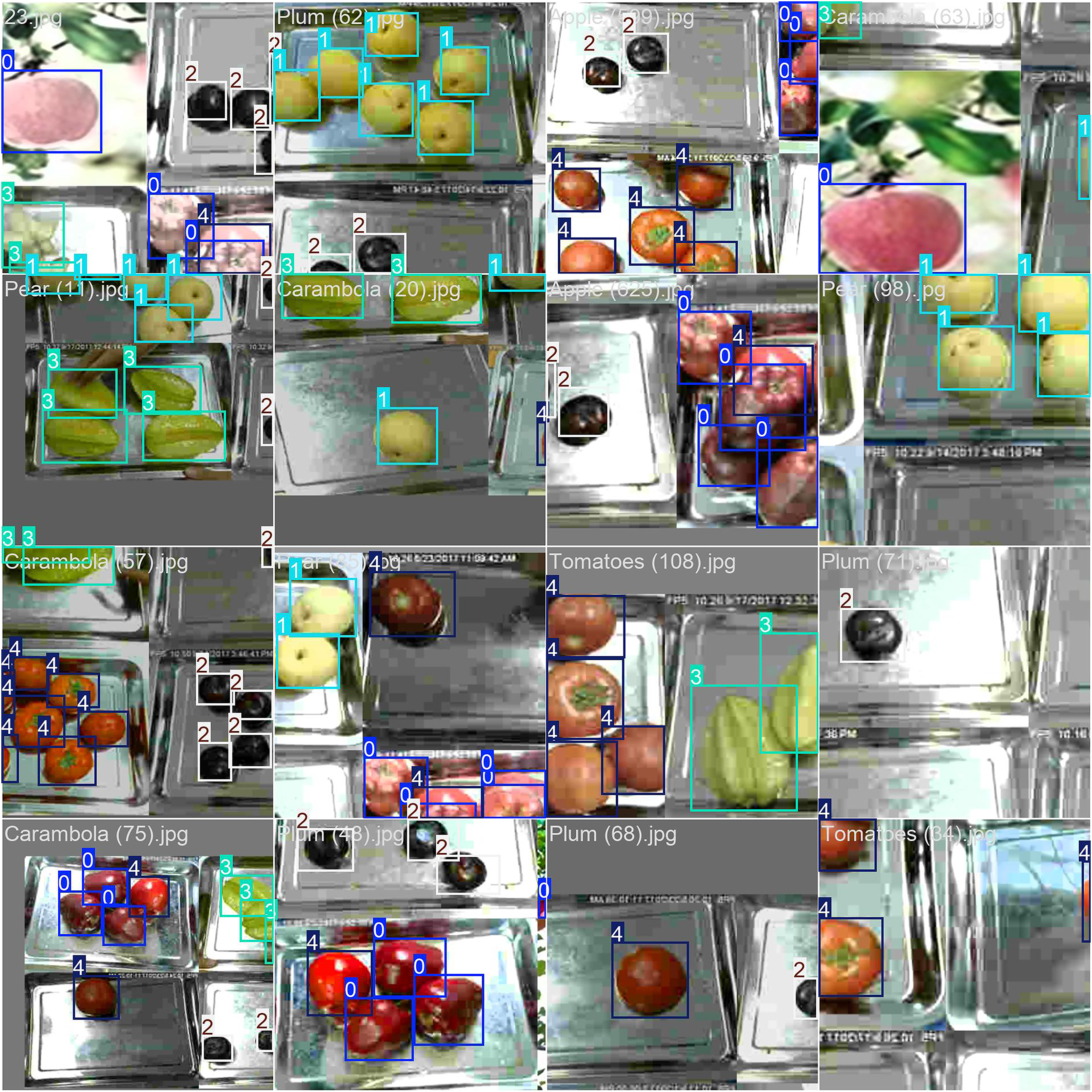
Application of the agricultural automation based on YOLO v8
The YOLO v8-based apple recognition and estimation framework presented in this study was well suited to the demands of modern agricultural automation systems. Its core advantages of real-time inference speed, high detection precision and strong robustness to small or partially occluded targets make it an ideal candidate for embedding directly on edge devices such as harvesting robots, unmanned aerial vehicles (UAVs) and conveyor-belt inspection stations. In our experiments (Table 3), the model achieved a mean average precision (mAP) of 95.0% and an F1-score of 93.45% under complex orchard conditions, and it outperformed classical CNN backbones such as VGG, ResNet and MobileNet. These performance gains resulted from YOLO v8’s optimized network architecture, which featured dynamic anchor assignment, improved feature-pyramid fusion and a streamlined head design. These architectural improvements were complemented by targeted data-augmentation strategies, including HSV jitter, random occlusion simulation and multi-scale mosaic stitching. Together, these techniques enhance robustness against illumination changes, fruit overlap and background clutter.
Although our system has not yet been deployed, it is anticipated that it could be integrated into three key automation scenarios. First, automated harvesting platforms could leverage on-board NVIDIA Jetson modules to perform continuous, real-time detection of ripe apples by applying the HSV-based ripeness classifier alongside YOLO v8’s bounding-box outputs. This would enable selective picking, reduce labor costs and minimize fruit damage. Second, in postharvest grading lines, conveyor belts equipped with RGB-D cameras and the 3D weight-estimation module could non-destructively sort fruit by both maturity level and estimated mass, thereby streamlining packaging and logistics. Finally, field-scale monitoring could be achieved by mounting lightweight inference units on UAVs or fixed-camera towers; these systems would survey large orchard areas, automatically map fruit density and health status, and feed geotagged yield estimates into precision-agriculture platforms to support adaptive irrigation, fertilization and pest-management decisions. Future studies will delve into the feasibility of hardware deployment in depth.
Despite these clear benefits, certain challenges remain to be addressed before widespread adoption. Performance may degrade in extreme weather conditions such as heavy rain or dense fog, unless additional sensor modalities are incorporated. The computational demands of the current model, although modest compared to earlier YOLO versions, still require careful hardware selection for fully autonomous mobile robots. Promising research directions include further lightweighting of the network through structured pruning or knowledge distillation and multi-sensor fusion approaches that combine RGB, hyperspectral and Light Detection and Ranging (LiDAR) data to extend detection into low-visibility conditions. Continuing to refine both the algorithmic and system-integration aspects ensures that YOLO v8-based frameworks play a pivotal role in realizing fully autonomous, intelligent orchards of the near future.
Failed instance
Despite optimizations in data augmentation and model training, the YOLO v8 model still encounters failures in real-world scenarios with complex backgrounds. These errors are not due to inherent issues within YOLO v8 architecture, but rather stem from a lack of sufficient and diverse data in the training dataset. Factors such as occlusion, varying lighting conditions, and image blurring hinder the model’s ability to accurately identify apples. As shown in the error samples in Figs. 14A–14D, the model often fails to detect apples properly, and in some cases, misidentifies the fruit. This suggests that the dataset’s relatively limited number of apple images, coupled with inadequate representation of diverse background scenarios, restricts the model’s ability to generalize to new, unseen environments. When exposed to backgrounds not included in the training set, the model struggles to make accurate predictions. By thoroughly analyzing and addressing these failure cases, the model’s performance and adaptability can be progressively enhanced, improving its suitability for apple-recognition tasks in complex settings.
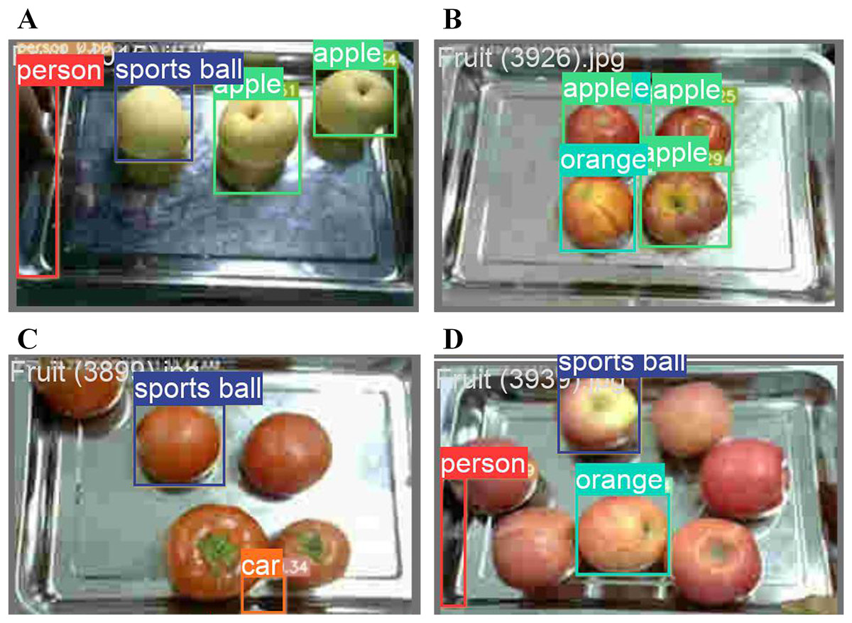
Figure 14: Model identification error samples.
(A, C and D) Shape similarity, (B) similar color.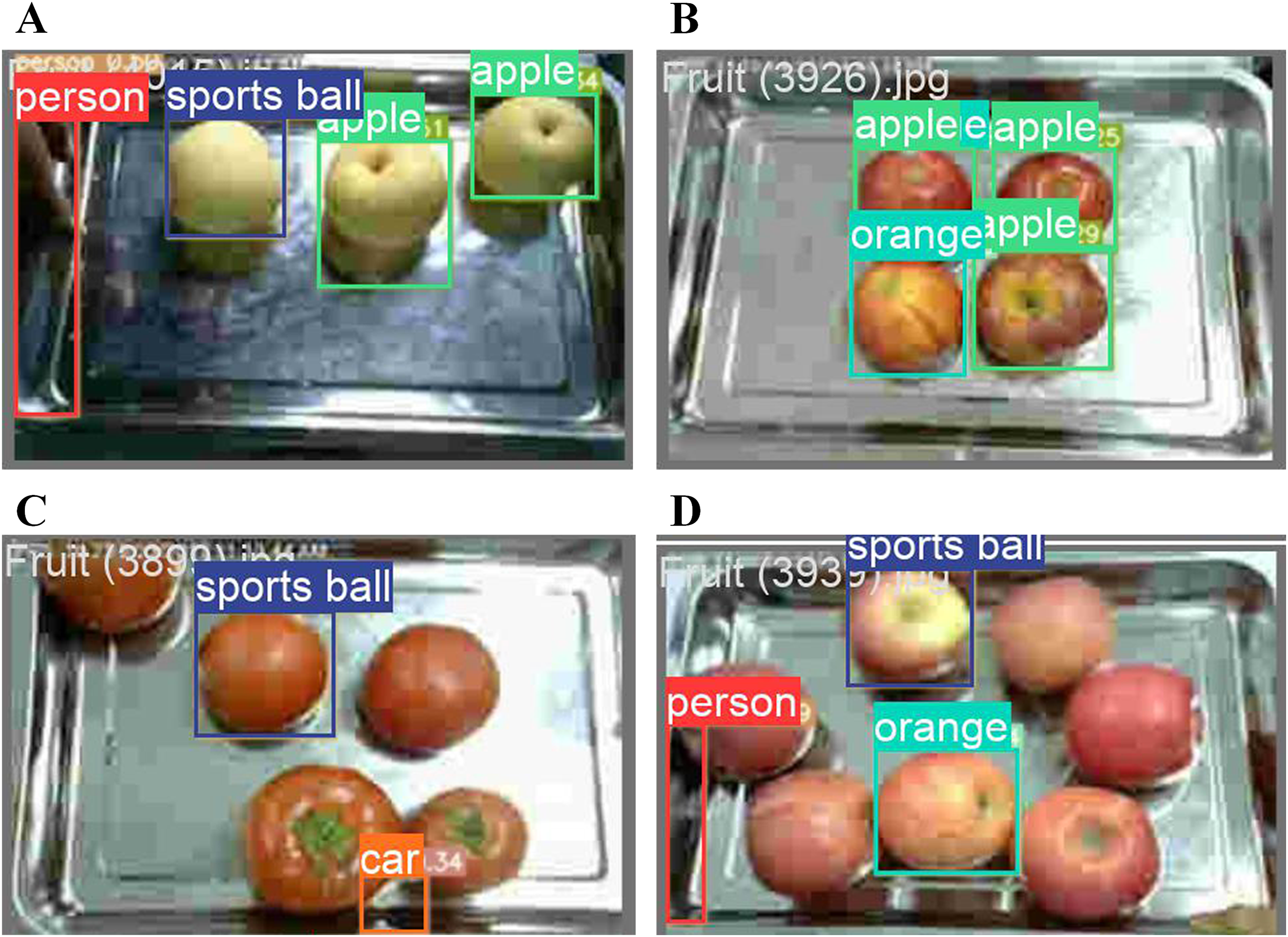
To overcome these limitations, it is necessary to enrich the training corpus with more varied and representative samples. One promising strategy is to leverage synthetic image generation techniques, which can systematically produce high-fidelity apple scenes under controlled variations of illumination, occlusion and background complexity. By combining real-world images with synthetic augmentations, we aim to expand the model’s exposure to rare or challenging conditions that are difficult to capture in the field.
In our current automation framework, the YOLO v8 model is trained exclusively on real-world orchard images to detect and localize apples in complex field conditions. Looking ahead, recent advances in large-language-model (LLM)-driven synthetic image generation offer a powerful means to implement this strategy. LLMs can generate diverse, realistic apple images that simulate a wide range of environmental factors. By incorporating LLM-generated images alongside real data, we expect to mitigate overfitting, enhance detector robustness and improve generalizability in data-scarce orchard environments. Future work will therefore investigate the integration of these synthetic samples and other multimodal inputs into our YOLO v8 pipeline to further boost detection accuracy and support more reliable automated apple picking systems.
Conclusion
This study proposes a solution to apple recognition by combining the YOLO v8 recognition model with the HSV color space. Apple image data from natural environments were collected and preprocessed, including grayscale conversion and Gaussian filtering for noise reduction. Edge detection was then performed using the Canny and Sobel operators, followed by apple identification with the YOLO v8 model. Apple maturity was assessed by utilizing both the HSV and RGB models to estimate maturity levels from the images. The apple weight was predicted using the proposed model. Finally, through color feature extraction and YOLO v8, apples were accurately identified among other fruits.
The YOLO v8 model demonstrates a low loss and achieves 95% mAP on this dataset, indicating its high accuracy in detecting and recognizing apples in complex backgrounds. The model also exhibits strong generalization across apples of varying sizes and degrees of occlusion. Compared to the best-performing algorithm, VGG, YOLO v8 shows an improvement of 0.14% in mAP, a 2.6% increase in accuracy, and a 0.58-point increase in F1-score. In terms of both speed and accuracy, YOLO v8 outperforms alternative models, enabling rapid and precise apple detection. This enhancement supports better understanding of apple attributes such as quantity, location, maturity, and weight, which in turn improves robotic recognition precision and harvesting efficiency. However, real-time deployment in large-scale scenarios requires significant computational resources. Additionally, the model may face challenges in generalization when applied to diverse apple varieties and environmental conditions.
Supplemental Information
Original dataset of apple images captured under complex background conditions, used for training and validating the YOLO v8 model. The images demonstrate various lighting conditions, occlusion scenarios, and natural orchard environments.
Four datasets from YOLO v8 model analysis.
(1) Apple counts per image, (2) Spatial coordinates (X, Y) of detected apples, (3) Maturity indices for spatial distribution analysis, and (4) Quality metrics including area and estimated weight for each apple.