
Enhanced Convolutional Neural Network (CNN)-Long Short-Term Memory (LSTM) attention model with adaptive loss for lithium-ion battery state of health estimation
- Published
- Accepted
- Received
- Academic Editor
- Arun Somani
- Subject Areas
- Algorithms and Analysis of Algorithms, Artificial Intelligence, Data Mining and Machine Learning, Scientific Computing and Simulation
- Keywords
- Lithium-ion battery, State of health (SOH), UGABO, MSAWH loss, Model predictive control (MPC), Data augmentation
- Copyright
- © 2025 Liao et al.
- Licence
- This is an open access article distributed under the terms of the Creative Commons Attribution License, which permits unrestricted use, distribution, reproduction and adaptation in any medium and for any purpose provided that it is properly attributed. For attribution, the original author(s), title, publication source (PeerJ Computer Science) and either DOI or URL of the article must be cited.
- Cite this article
- 2025. Enhanced Convolutional Neural Network (CNN)-Long Short-Term Memory (LSTM) attention model with adaptive loss for lithium-ion battery state of health estimation. PeerJ Computer Science 11:e3006 https://doi.org/10.7717/peerj-cs.3006
Abstract
This study proposes an enhanced deep learning framework for accurately estimating the state of health (SOH) of lithium-ion batteries (LIBs), leveraging a refined Convolutional Neural Network (CNN)-Long Short-Term Memory (LSTM)-Attention architecture. To improve prediction accuracy and robustness, a novel Multi-Scale Adaptive Wasserstein-Huber Loss (MSAWH Loss) is introduced, which combines the strengths of Huber loss and multi-scale Wasserstein distance to effectively handle outliers and capture complex degradation patterns. Furthermore, an Uncertainty-Guided Adaptive Bayesian Optimization (UGABO) algorithm is employed to optimize model hyperparameters, achieving efficient convergence in high-dimensional and noisy parameter spaces while maintaining a balance between exploration and exploitation. To enhance generalization, four complementary data augmentation techniques—linear interpolation, data slicing, sequence flipping, and cross-sample mixing—are applied to the National Aeronautics and Space Administration (NASA) charge-discharge dataset, significantly enriching the training data. Additionally, a Model Predictive Control (MPC) mechanism is integrated to correct long-horizon prediction errors, dynamically refining outputs based on recent deviations and maintaining consistency with real-world battery constraints. Experimental results demonstrate that the proposed framework outperforms baseline models, achieving a 20.6% reduction in mean absolute error (MAE), an 18.6% reduction in root mean squared error (RMSE), and a 0.1% improvement in R-squared (R2). These findings highlight the effectiveness of integrating adaptive loss design, automated hyperparameter optimization, strategic data augmentation, and feedback-based error correction in advancing SOH prediction performance for lithium-ion batteries.
Introduction
The growing global concern over climate change is primarily driven by severe environmental degradation caused by fossil fuel combustion and the depletion of non-renewable energy resources. This situation underscores the urgent need for clean energy alternatives and high-efficiency energy storage systems. Lithium-ion batteries (LIBs) have emerged as a cornerstone in energy storage solutions and electric vehicles due to their wide operational temperature range, long cycle life, high energy density, and eco-friendly characteristics during use (Rial, 2024). Their superior lifespan, energy efficiency, and low environmental impact have made LIBs indispensable components in electric vehicles (EVs) (Li et al., 2019). Meanwhile, artificial intelligence (AI) has been increasingly applied in a wide range of energy-related fields, including the design of novel materials and smart devices, highlighting its interdisciplinary potential beyond battery health prediction. In practical applications, the health of lithium-ion batteries directly influences the driving range, reliability, and safety of electric vehicles, making accurate state estimation essential for both users and manufacturers. However, LIBs are not without limitations. Vulnerabilities to external factors, such as temperature and current fluctuations, coupled with rapid aging, remain significant challenges. A critical issue arises during repetitive battery cycles, where phenomena like lithium-ion deposition on the anode lead to the loss of active lithium, increased impedance, and a noticeable reduction in battery capacity. For example, uncontrolled degradation can reduce a battery’s capacity to hold charge, resulting in frequent recharging and reduced travel distances. If improperly managed, these issues can shorten the operational duration of EVs and pose potential safety risks. Therefore, it is crucial to develop techniques that can accurately and promptly assess and forecast the degradation behavior of LIBs (Guo et al., 2023).
Currently, most research on battery longevity and expected lifespan focuses on predicting battery capacity and internal resistance (Wang et al., 2021). Batteries are generally considered no longer suitable for use when their capacity drops to 80% of the initial value or when internal resistance doubles. However, both capacity and internal resistance are not directly measurable, making accurate and real-time state of health (SOH) estimation a key challenge. Accordingly, obtaining precise assessments of degradation states and remaining useful life (RUL) using measurable signals such as voltage, current, and temperature has become essential (Li et al., 2021).
In recent years, numerous researchers have explored the degradation characteristics and prediction of the RUL of LIBs, with data-driven models emerging as one of the most widely adopted approaches (Amiri et al., 2024). These models utilize historical data and advanced algorithms to predict and analyze battery behavior. Depending on the application scenarios and algorithms, data-driven models are generally classified into machine learning models, deep learning models, and statistical models (Ali et al., 2024).
Machine learning models have been extensively applied to battery SOH estimation, demonstrating specific strengths and limitations. For example, Tu et al. (2023) proposed a physics-informed hybrid model, in which a neural network leveraged outputs from a physical model to deliver accurate voltage predictions with low computational overhead. Similarly, Zhang et al. (2024b) introduced a cloud-based, in-situ battery life prediction framework that used a moving-window technique to extract aging-related features, thereby enabling reliable SOH predictions. Additionally, to determine the most effective method for SOH estimation, Korkmaz (2023) compared 18 machine learning methods for SOH estimation and identified optimal combinations for different scenarios. However, traditional machine learning methods often require manual feature extraction related to battery characteristics, which risks overlooking critical patterns. These methods also face challenges in modelling complex nonlinear relationships and handling large-scale datasets, limiting their predictive accuracy. More recent algorithms, such as Random Vector Functional Link (RVFL) and Active State Tracking Long Short-Term Memory (AST-LSTM), have attempted to overcome these constraints. Nevertheless, limitations remain: RVFL lacks strong feature extraction capabilities and struggles with modelling long-term dependencies (Sajid et al., 2024), while AST-LSTM’s performance heavily depends on the availability of high-quality datasets and task-specific parameters (Zhang et al., 2024b). These insights emphasize the need for more robust and adaptive solutions to address the complexities of SOH estimation.
With the rise of powerful Graphics Processing Units (GPUs), deep learning-based SOH estimation has shown great promise due to its capacity to model complex nonlinear systems adaptively to model complex nonlinear systems adaptively (Park et al., 2023). These advancements have driven significant progress in battery research and other fields (Ding et al., 2024). For instance, Van & Quang (2023) employed LSTM networks to predict the SOH and internal resistance of LIBs using experimental charging and discharging data, including voltage, current, temperature, and impedance. Building on this, Jia et al. (2024) proposed a hybrid Convolutional Neural Network (CNN)-Bidirectional Long Short-Term Memory (BiLSTM) model to estimate the RUL of LIBs, effectively addressing the issue of limited historical data. Chen et al. (2023) further proposed a Fusion-Fission Optimization (FuFI) method that integrates CNN with Bi-LSTM to capture both spatial and temporal data features, significantly improving SOH prediction accuracy.
Expanding on these advances, Mazzi, Sassi & Errahimi (2024) designed a hybrid deep learning model integrating CNN and Bidirectional Gated Recurrent Unit (BiGRU) networks for SOH estimation. In their framework, the 1D CNN processed input data (current, voltage, temperature) to extract essential features, while the BiGRU component captured temporal dependencies in sequential data. Despite these advancements, such deep learning models often focus on short-term data fluctuations and are limited in their capacity to model long-term dependencies effectively. To address this, Li et al. (2024) introduced a digital twin architecture leveraging Backpropagation Neural Network (BPNN) and CNN-LSTM-Attention networks for real-time capacity degradation tracking. The CNN-LSTM-Attention framework offers distinct advantages by combining CNNs for feature extraction from raw data, LSTMs for modelling long-term temporal dependencies, and attention mechanisms for identifying critical time steps and enhancing the model’s focus on key patterns. These components make CNN-LSTM-Attention particularly suitable for handling complex nonlinear relationships, massive datasets, and sequential data in battery SOH prediction. However, a key drawback of this model is its reliance on large volumes of high-quality data to fully capture the characteristics and behavior of LIBs. Insufficient or low-quality data can significantly hinder its performance, limiting its practical application. To mitigate this, data augmentation techniques were employed in this study, expanding the training dataset to improve the model’s ability to learn from both short- and long-term patterns, even under limited data conditions. These enhancements significantly improve the robustness and predictive accuracy of the CNN-LSTM-Attention framework.
Hyperparameter tuning is another pivotal factor that influences model effectiveness. Since their performance and generalization ability depend heavily on parameters such as the number of layers, learning rate, and batch size (Hanifi, Cammarono & Zare-Behtash, 2024). The model’s performance and generalization ability are greatly influenced by their specific configuration (Jiralerspong et al., 2023). Finding the optimal combination of these hyperparameters through simple manual tuning is often impractical. Because of the extensive hyperparameter space, manually tuning the model is not only labour-intensive and time-consuming but also likely to overlook the optimal configuration (Fakhouri et al., 2024). In deep learning, Bayesian optimization constructs a surrogate model and uses acquisition functions to select hyperparameter combinations, iteratively optimizing them to efficiently and automatically find the best hyperparameter settings (Baratchi et al., 2024). This approach can greatly improve the generalization ability and performance of deep learning models. Selvaraj & Vairavasundaram (2024) utilized hyperparameter tuning techniques based on Bayesian optimization algorithms to address the drawbacks of manually setting network parameters. However, traditional Bayesian optimization struggles in high-dimensional spaces and balancing exploration with exploitation, which can lead to either computational inefficiency or local optima. To address this, our work proposes a novel Uncertainty-Guided Adaptive Bayesian Optimization (UGABO), which dynamically balances exploration and exploitation and significantly improves convergence in noisy environments.
Equally important is the choice of loss function, which directly impacts prediction stability and error sensitivity (Mushava & Murray, 2024). Standard options such as mean squared error (MSE), mean absolute error (MAE), Huber, and Wasserstein loss each offer distinct benefits (Terven et al., 2023). Huber Loss combines the advantages of MSE and MAE, making it suitable for scenarios where both small errors and outliers need to be handled (Yang et al., 2024). Zhang et al. (2024d) presented a Wasserstein distance-based Quantile Huber (QH) loss function, integrating Huber and quantile regression losses, outperforms conventional MAE and MSE in optimizing SOH estimation. Although this loss function combines the advantages of MSE and MAE, it does not account for the influence of the parameter in the Huber loss function. Additionally, selecting the appropriate quantile parameter requires experience and experimentation, which significantly impacts the model’s predictive ability. Building upon this, we introduce the Multi-Scale Adaptive Wasserstein-Huber Loss (MSAWH Loss) to deliver superior performance across varying error distributions.
In addition to improvements in deep model architectures, some researchers have also studied error correction mechanisms in lithium battery state prediction. In the article by Zhang et al. (2024c), the author proposed a novel algorithm called Cascaded Robust Control-Supportive Hybrid Extended Kalman Filter (CRC-SHEKF), which combines Sage Husa adaptive methods with enhanced Cauchy robust correction to improve SOH estimation for lithium-ion batteries, addressing noise estimation inaccuracies. However, lithium battery systems face multiple physical constraints, such as voltage, current, and temperature limits (Zheng et al., 2024). Traditional prediction methods often struggle to simultaneously account for these constraints, and errors can accumulate over long-term predictions, causing deviations from true values. This study addresses error correction challenges using a novel method based on MPC. Our solution introduces a MPC strategy with a lookahead mechanism to dynamically revise prediction trajectories, ensuring physical consistency and long-term stability.
In light of the latest developments in SOH estimation frameworks, several studies have introduced novel learning paradigms. For instance, one recent work proposed a global–local context embedding learning strategy that integrates multiscale convolutional streams to extract deep spatial features and guide time series prediction without relying on sequence dependency (Bao et al., 2023). Another study introduced a multiple aging factor interactive learning framework that models feature correlations in an interactive manner and encodes aging-related information using an enhanced perceptron network (Bao et al., 2025). These works underscore the growing emphasis on integrating multi-dimensional relationships and structural innovations in battery SOH estimation.
To better position our study within the broader research landscape, Table 1 presents a comparative summary of eight representative SOH estimation methods, highlighting their core techniques, advantages, and limitations.
| Author | Methodology | Feature extraction | Time-series modeling | Uncertainty handling | Data requirements | Optimization | Main limitation |
|---|---|---|---|---|---|---|---|
| Tu et al. (2023) | Hybrid physics-ML | Engineered | No | No | Low | Fixed | Low flexibility |
| Jia et al. (2024) | Digital twin (CNN-LSTM-Attn) | Automatic + Feature selection | Yes | No | High | Manual | Dataset dependency |
| Chen et al. (2023) | CNN + BiLSTM + FuFi | Automatic | Yes (BiLSTM) | No | Medium | Manual | Lacks uncertainty modeling |
| Mazzi, Sassi & Errahimi (2024) | CNN-BiGRU | Automatic | Yes (BiGRU) | No | Medium | Bayesian Opt. | Short-term bias |
| Li et al. (2024) | CNN-LSTM-attention | Automatic | Yes (LSTM + Attn) | Partially | High | Grid search | Needs clean long-term data |
| Selvaraj & Vairavasundaram (2024) | CNN-BO | Automatic | Yes | No | Medium | UGABO | BO efficiency in high-dim |
| Zhang et al. (2024d) | QH-Loss based CNN | Automatic | Partial (CNN) | Yes (Quantile) | Medium | Grid Search | Weak interpretability |
| Zhang et al. (2024c) | CRC-SHEKF | Engineered | No | Yes (Noise) | Low | Fixed | Low adaptability |
| Our work | CNN-LSTM-Attn + UGABO + MSAWH + MPC | Automatic | Yes | Yes | Medium | Adaptive BO | High performance, but complexity |
Inspired by the aforementioned research advancements and existing challenges, this study proposes significant enhancements to the CNN-LSTM-Attention framework, focusing on dataset processing, hyperparameter optimization, loss function design, and error correction mechanisms. The primary innovations of this work are as follows:
-
(1)
Comprehensive Dataset Augmentation: Based on the widely used National Aeronautics and Space Administration (NASA) charge-discharge dataset, this study constructs enriched training datasets through the integration of four distinct augmentation techniques—linear interpolation, data slicing, data flipping, and cross-validation sampling. Compared to previous works that typically adopt only one augmentation strategy, our approach combines these complementary methods to significantly improve the diversity, generalizability, and robustness of the training process.
-
(2)
Uncertainty-Guided Adaptive Bayesian Optimization (UGABO): To address the challenge of noisy and uncertain objective functions in hyperparameter tuning, we introduce UGABO—an adaptive optimization algorithm that dynamically balances exploration and exploitation. This method enables more efficient convergence in high-dimensional, noise-prone parameter spaces, leading to consistently superior model performance. To the best of our knowledge, this is the first application of UGABO in the SOH prediction domain.
-
(3)
Multi-Scale Adaptive Wasserstein-Huber Loss (MSAWH Loss): A novel loss function is proposed that fuses the strengths of Huber loss (for outlier robustness) with multi-scale Wasserstein distance (for distribution-aware sensitivity). This hybrid formulation allows for adaptive penalization of prediction errors at multiple scales, resulting in enhanced accuracy, stability, and resilience against distribution shifts or sensor noise.
-
(4)
Error Correction with Model Predictive Control (MPC): To mitigate long-horizon prediction drift and accumulation of deviation errors, this study incorporates an MPC-based correction mechanism. By leveraging feedback control, the model dynamically adjusts its predictions based on recent errors, ensuring trajectory smoothness and consistency with real-world battery constraints (e.g., voltage, current, temperature), thus improving practical reliability.
Materials and Methods
Materials
The proposed model was implemented using Python 3.11.5 with TensorFlow as the primary deep learning framework. All experiments were conducted in an Anaconda-managed environment. The experiments were executed on a high-performance cloud computing platform (AutoDL), equipped with a 16-core Intel Xeon(R) Gold 6430 CPU, 120 GB of RAM, and an NVIDIA RTX 4090 GPU with 24 GB memory. This setup ensured efficient training and evaluation of deep learning models under large-scale battery data. All dependencies are documented in the provided GitHub repository at https://github.com/Benmoshangsang/SOH-predict-2025. The repository includes modular code for each experimental task, including baseline training, loss function comparison, hyperparameter tuning, ablation studies, and data augmentation. Utility scripts for preprocessing, parameter configuration, and model definition are also included. The raw battery dataset used in this study was sourced from NASA, comprising voltage, current, and temperature measurements under various operating conditions. To improve model robustness and generalization, three augmentation strategies—slicing, flipping, and linear interpolation—were applied to generate synthetic data. All raw and augmented datasets, along with model outputs and results, are accessible via Zenodo at https://doi.org/10.5281/zenodo.15239011.
Model performance was rigorously evaluated using a comprehensive suite of regression-based metrics, including: MAE, MSE, mean absolute percentage error (MAPE), root mean square error (RMSE), R-squared (R2), centered root mean square difference (CRMSD), median absolute difference (MAD), and normalized RMSE (nRMSE). These metrics were carefully selected to capture both absolute and relative prediction accuracy, and were uniformly applied across all experimental modules to ensure consistency and comparability.
The following sections detail the core methodological components employed in this study, including the data augmentation pipeline, the CNN-LSTM architecture enhanced with attention mechanisms, the ablation strategy, and the hyperparameter optimization process.
Data augmentation
Linear interpolation is a widely used technique for estimating missing values in lithium-ion battery datasets by generating intermediate data points between existing observations (Xiong et al., 2024). For SOH prediction, given two known data points ( , ) and ( , ), representing voltage at times and , the linear interpolation formula is:
(1) where is a time point between and , and is the predicted voltage value. represents the voltage at the starting time , and represents the voltage at the ending time . This technique is applied to various parameters including voltage, current, capacity, and temperature to produce more continuous and smooth data. This enhanced dataset contributes to improving the model’s SOH estimation accuracy by providing a more thorough depiction of battery behaviour over time.
Slicing is a data preprocessing technique particularly effective for time series analysis. It involves segmenting the original long-sequence data into multiple fixed-length subsequences, thereby enabling downstream machine learning models to more efficiently process and analyse the temporal patterns within these segments (Xie et al., 2024).
Given the original time series data , where indicates the length of the sequence, the subsequence after slicing is defined as:
(2) where represents the slicing length, which indicates the length of each subsequence after slicing. S indicates slicing step, representing the number of steps to move forward in the original sequence each time a new subsequence is created. is the i-th subsequence obtained after slicing. represent elements of the i-th subsequence, extracted from the original sequence according to the slicing step S and slicing length .
This method facilitates the identification of localized patterns and trends within specific time windows, enabling the model to more effectively learn temporal dynamics. It is particularly valuable for detecting short-term variations in battery performance that may signal longer-term degradation trajectories.
Flipping is a data augmentation technique that involves reversing the order of a time series sequence. This technique helps to create additional training samples from the original data, enhancing the diversity and robustness of the training set (Chou & Nguyen, 2024).
Given the original time series data, for a time series data , the flipped sequence is:
(3) where represents the original time series data, and is the length of the sequence, indicating the total number of elements in the sequence. is the flipped or reversed sequence of , starting from the last element and going to the first.
This method applies to all parameters (voltage, current, temperature) to mimic various charging and discharging cycles. Flipping increases the dataset’s diversity, providing the model with a wider range of scenarios to learn from, which enhances its generalization capability and robustness in real-world applications.
Cross-validation is a technique for assessing model performance by partitioning the dataset into several subsets. The model is methodically trained and validated on various combinations of these subsets. This approach helps evaluate the model’s effectiveness and its ability to generalize to new, unseen data (Ahmadzadeh, Zahrai & Bitaraf, 2024).
Given a dataset D with N samples, and K folds, cross-validation involves:
(1) Split the D into K equally sized subsets .
(2) For each fold k (where k = ), designate as the validation set and utilize the remaining K − 1 subsets as the training set.
(3) Compute the evaluation metric, such as MAE or MSE, for each fold, and then average the results across all folds.
This method is applied across all relevant parameters—voltage, current, and temperature—to construct a composite dataset that captures a diverse range of operational conditions. The crossing strategy enhances the model’s ability to generalize by exposing it to mixed behavioural patterns, enabling better adaptation to different battery states and environmental scenarios. By integrating characteristics from multiple data sequences, this technique introduces greater variability and complexity, which in turn improves the deep learning model’s capacity to manage heterogeneous real-world conditions with enhanced robustness and predictive accuracy.
Uncertainty-guided adaptive Bayesian optimization (UGABO)
UGABO is a strategy that combines uncertainty estimation with adaptive exploration-exploitation trade-offs in Bayesian optimization. The core idea is to dynamically adjust the balance between exploration and exploitation by guiding the process based on uncertainty estimates, thereby achieving more efficient optimization (Zangirolami & Borrotti, 2024). UGABO begins with initial hyperparameter settings and iteratively adjusts them using optimization algorithms. This approach gradually converges to an optimal configuration, balancing accuracy, robustness, and computational efficiency.
Gaussian process regression (GPR) is commonly used to model the objective function in Bayesian optimization. It provides a probabilistic framework to estimate the function and its uncertainty (Li et al., 2024).
Given a set of observed data points , where each pair represents an input and its corresponding observed output . represents the i-th input in the observed dataset, and is the corresponding function value or observed output for input . The corresponding function value, a gaussian process assumes that the function follows a multivariate normal distribution over any finite set of points:
(4) where represents the target function, representing the function value at the input x. denotes that is modeled as a Gaussian process with a mean function and a covariance function . represents Mean function (often assumed to be zero) and indicates Covariance function (kernel function), such as the Radial Basis Function (RBF) kernel.
Acquisition functions guide the selection of the next evaluation point by balancing exploration and exploitation (Duankhan et al., 2024). The Upper Confidence Bound (UCB) acquisition function incorporates both the mean and the uncertainty of the prediction, controlled by a parameter :
(5) where represents the UCB acquisition function value, which evaluates the potential of selecting point x. denotes the predicted mean at point x. represents the predicted uncertainty (standard deviation) at point x. is a parameter that controls the trade-off between exploration and exploitation, higher values of encourage exploration by giving more weight to the uncertainty term , and lower values of favor exploitation by focusing more on areas with high predicted mean .
UGABO dynamically adjusts the exploration-exploitation balance based on the uncertainty estimates. This ensures that the algorithm focuses more on exploration in regions of high uncertainty and on exploitation (Daliri et al., 2024).
The trade-off parameter can be dynamically adjusted using the maximum uncertainty :
(6) where represents the trade-off parameter at iteration step t, controlling the balance between exploration and exploitation during the optimization process. indicates initial trade-off parameter, denotes the maximum uncertainty observed in the current iteration, guiding the adjustment of the trade-off parameter to favor exploration when uncertainty is high. represents the uncertainty associated with the prediction at point x during the n-th iteration, used to normalize the trade-off adjustment.
The complete UGABO process is illustrated in Fig. 1.
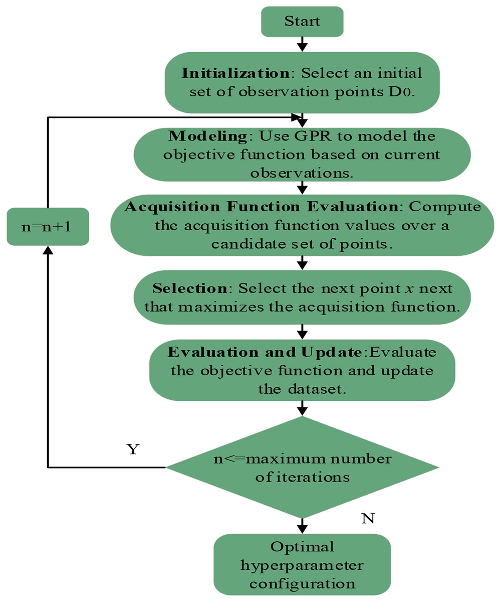
Figure 1: Detailed workflow of the uncertainty-guided adaptive Bayesian optimization (UGABO) algorithm for hyperparameter tuning.
The complete process of UGABO. It includes steps such as initialization of observation points, modeling the objective function using Gaussian process regression (GPR), evaluating acquisition functions, selecting optimal points, and iteratively updating until reaching the stopping criterion for hyperparameter optimization.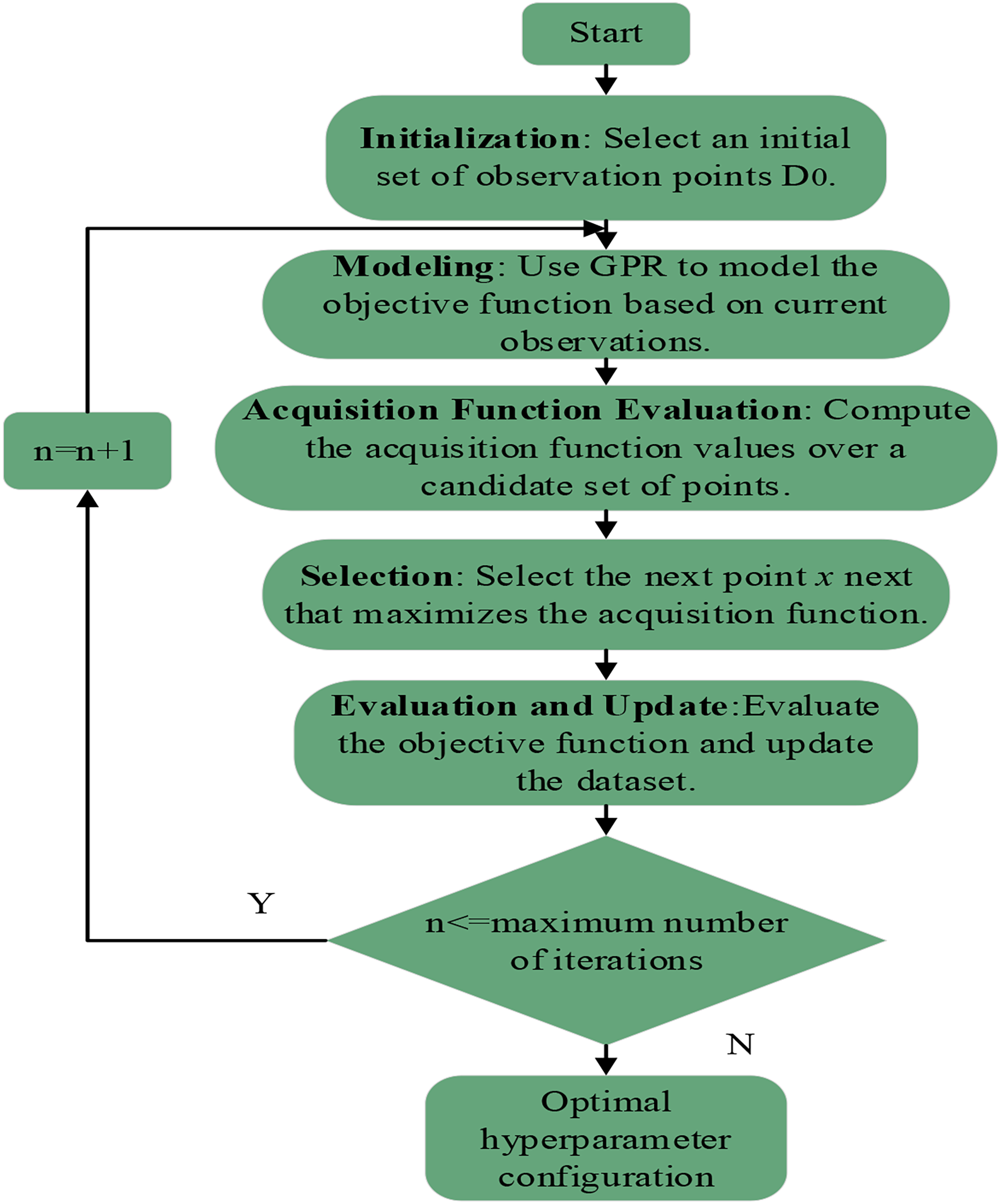
Multi-scale adaptive Wasserstein-Huber loss (MSAWH loss)
MSAWH is a method that dynamically adjusts the parameter of the Huber loss and incorporates multi-scale Wasserstein distances, aiming to build a more robust and flexible loss function by combining the strengths of both components, the specific workflow is shown in Fig. 2.
Figure 2: Workflow of the multi-scale adaptive Wasserstein-Huber (MSAWH) loss function for gradient-based model optimization.
The workflow of the MSAWH loss optimization. The process involves calculating dynamically adjusted Huber loss and multi-scale Wasserstein distance, followed by gradient computation and parameter update through backpropagation, iterating until convergence.
The Huber loss function is defined as:
(7) where denotes the Huber loss function, is the error term, the difference between the predicted value and the true value, and is the threshold that determines whether the loss behaves quadratically (for small errors) or linearly (for larger errors).
During training, the parameter is dynamically adjusted based on the statistical properties of the errors, allowing it to adaptively change to provide more appropriate penalties across different error ranges. By dynamically adjusting the parameter of the Huber loss, the model can handle outliers more robustly.
Calculation of the Wasserstein distance at different scales to capture distributional differences at various levels is given as follows (You, Shung & Giuffrè, 2024).
The Wasserstein distance is defined as:
(8) where represents the Wasserstein distance between the probability distributions p and q, denotes the infimum (greatest lower bound). It is used here to find the minimum value of the expected distance over all possible joint distributions. represents a joint distribution over the product space of x and y, where the marginals are p and q respectively. denotes the set of all joint distributions with marginals and . represents the expected value (expectation) with respect to the joint distribution γ. It is the average value of the function when pairs are sampled according to γ, and is the distance metric between points and .
Multi-scale Wasserstein distances capture distributional differences at various scales, enhancing the model’s sensitivity to information across different levels.
Combine the multi-scale Wasserstein distance with the adaptively adjusted Huber loss to form a new loss function:
(9) where represents the combined loss function, specifically designed to integrate the MSAWH loss. This function combines the Wasserstein distance and Huber loss components to adapt to various data distributions. and are weighting parameters that control the influence of the Huber loss and Wasserstein distance components in the combined loss function. represents the sum of Wasserstein distances calculated at different scales, with each term in the sum being weighted by , and is the weight for the Wasserstein distance at the i-th scale, allowing the model to adjust the importance of each scale’s contribution to the total loss. denotes the Wasserstein distance between distributions p and q at the i-th scale. This term measures the distance between distributions at multiple resolutions or granularities.
Combining Wasserstein distance with Huber loss provides a flexible framework that can adapt to different types of data distributions and error characteristics.
Model predictive control (MPC) error correction
The MPC method is primarily used for prediction and control issues in dynamic systems (Zhao et al., 2024b). In this article, MPC is used to adjust the predicted time series data to more accurately match the actual values. Specifically, it dynamically adjusts predicted values to bring them closer to observed actual values. The optimization of the cost function reduces the error between predicted and actual values. During this process, it also smooths out anomalies in the predicted values (Gu, Wang & Liu, 2024).
In the MPC control approach, the cost function is mainly utilized to assess the discrepancy between the predicted values and the actual values (Han, Park & Lee, 2024). The formula is:
(10) where represents the cost function, which is used to quantify the discrepancy between the predicted values and the actual values over a specified prediction horizon. represents the time step within the predicted horizon. N is the prediction horizon (the total number of future steps over which the cost function is evaluated). represents the actual value or ground truth for the target variable at time step t, represents the predicted value at time step t, represents the adjustment value applied at time step t, which is used to fine-tune or correct the prediction.
CNN-LSTM-Attention
The CNN is a deep learning architecture specifically designed to process data with a grid-like topology, such as images and time series (Zeghina et al., 2024). By leveraging local connections and weight sharing, CNNs effectively extract spatial or temporal features from input data, reducing the number of parameters and computational complexity (Zhang et al., 2024a). Their primary function is to automatically extract and learn high-level features from data, enabling the model to achieve high accuracy and efficiency in tasks such as classification, detection, and prediction (Kheddar et al., 2024).
A typical 1D-CNN consists of an input layer, a convolutional layer, a pooling layer, a fully connected layer, and an output layer. The input layer acts as the gateway for data. In the convolutional layer, features are extracted using a particular convolutional kernel, often referred to as a feature detector. The feature extraction process follows this formula:
(11) where represents the output of the convolution operation, denotes the input feature map, refers to the convolutional kernel, corresponds to the height of the convolutional kernel, respectively, and denotes the position of the output, is the index variable used in the summation, representing the positions within the convolutional kernel as it slides over the input feature map.
Ultimately, the CNN architecture combines outputs from various convolutional layers, utilizing Dropout and Batch Normalization to boost the model’s generalization ability and stability. This structure ensures effective learning from both temporal data and local features, while enhancing prediction performance through the fusion of multi-level features (Man et al., 2024).
LSTM is a variant of recurrent neural networks (RNNs) specifically designed to capture long-term dependencies within sequential data (Ehteram et al., 2024). LSTMs overcome the problems of vanishing and exploding gradients found in traditional RNNs by incorporating memory cells and gating mechanisms, which are specialized units designed for this purpose (Al-Selwi et al., 2024). In the CNN-LSTM-Attention model, LSTM is used to process time series data, such as voltage, current, and temperature over time. LSTM can capture the temporal dependencies in these sequences, providing more accurate predictions (He et al., 2024). An LSTM network consists of four key components: the input gate, forget gate, output gate, and cell state (Ehteram et al., 2024). Each component is vital for the LSTM’s operation, but the cell state stands out as the most critical. The cell state functions like a conveyor belt, enabling information to pass through multiple time steps without alteration, which is essential for preserving long-term dependencies (Zhao et al., 2024a). LSTM is governed by the cell state formula:
(12) where represents the cell state at the current time step t, t is the time step in the sequence, and denotes the forget gate’s activation vector at time step t, which determines how much of the previous cell state should be retained, is the cell state at the previous time step (t − 1), is the input gate’s activation vector at time step t and is the candidate cell state at time step t.
In the CNN-LSTM-Attention model, LSTM plays a crucial role in capturing long-term dependencies in time series data. By combining CNN and Attention mechanisms, the model can more accurately predict the SOH of lithium batteries. The final outputs of the model include predicted SOH (make sure consistent) values and relevant evaluation metrics to assess the model’s performance.
The Attention mechanism is an advanced technique employed to improve the efficiency of models when processing sequential datasets. This approach allows the model to focus more on the relevant parts of the data by assigning varying levels of importance to different segments of the input sequence (Hassanin et al., 2024). By dynamically assigning different weights to various segments of the input sequence, this approach allows the model to focus on the most relevant information for the current task (Guo et al., 2024). For predicting the SOH in lithium batteries, the Attention mechanism can boost the performance of the CNN-GRU model by highlighting the time steps most relevant to SOH variations, thereby increasing the accuracy of the predictions (Du et al., 2024).
The core of the Attention mechanism lies in its ability to dynamically adjust the importance of input information, making the model more accurate in time series prediction. In lithium battery SOH prediction, the Attention mechanism helps the model better identify and utilize important time step data, thereby improving prediction performance and accuracy.
Evaluation metrics for prediction performance
To accurately quantify the deviation between forecasted outcomes and actual values, it is essential to implement appropriate performance assessment metrics. Let y = represents the vector of actual values, with the average value denoted by . The vector representing the forecasted values is denoted by , and the relationship between them is captured by relevant assessment metrics. The main assessment metrics are listed below:
MAE:
(13)
MSE:
(14)
MAPE:
(15)
RMSE:
(16)
R2:
(17)
CRMSD:
(18)
MAD:
(19)
nRMSE:
(20)
Process flow of UGABO-CNN LSTM Attention-MSAWH Loss-MPC model
The detailed workflow of the UGABO-CNN-LSTM-Attention-MSAWH Loss-MPC model is depicted in Fig. 3, outlining data preparation, model training, prediction, and evaluation stages. The process ensures a structured and reproducible approach for LIB SOH evaluation.
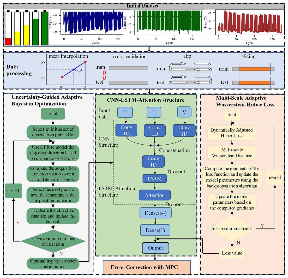
Figure 3: Integrated workflow of the proposed UGABO-CNN-LSTM-Attention model incorporating data augmentation, uncertainty-guided Bayesian optimization, MSAWH loss, and MPC-based.
The full model pipeline integrating UGABO, CNN-LSTM-Attention, and MSAWH loss. It starts from raw dataset visualization, proceeds through data augmentation techniques (interpolation, cross-validation, flipping, slicing), shows the model architecture including convolutional layers and attention modules, and concludes with the error correction mechanism using MPC.
Results
To evaluate the practicality and effectiveness of the proposed LIB SOH prediction framework, this section presents a comprehensive experimental validation. Starting with the NASA dataset as the baseline, the raw data underwent systematic augmentation to generate four new datasets with improved diversity and generalizability. These augmented datasets were subsequently divided into training, validation, and testing subsets to facilitate robust model evaluation. The enhanced datasets were then fed into the proposed prediction framework for both training and testing. Finally, the results were thoroughly analysed and benchmarked against alternative approaches to ensure a rigorous and objective assessment of the framework’s predictive performance.
Raw data description
To analyse the degradation performance of LIBs in electric vehicles and support the development of deep learning prediction models, the NASA lithium battery dataset serves as the foundation data source (Saha & Goebel, 2007). This dataset includes four batteries: B0005, B0006, B0007, and B00018. The basic testing parameters of these four batteries are summarized in Table 2. These batteries are initially charged in a constant current (CC) mode at 1.5 A until they reach 4.2 V, then charged in a constant voltage (CV) mode until the current decreases to 20 mA. The discharge process occurs in CC mode at 2 A until the voltages of batteries 5, 6, 7, and 18 drop to 2.7, 2.5, 2.2, and 2.5 V, respectively.
| Model | Temperature/°C | Charging current/A | Discharging current/A | Cut-off voltage/V |
|---|---|---|---|---|
| B0005 | 24 | 1.5 | 2 | 2.7 |
| B0006 | 24 | 1.5 | 2 | 2.5 |
| B0007 | 24 | 1.5 | 2 | 2.2 |
| B0018 | 24 | 1.5 | 2 | 2.5 |
The battery is subjected to continuous charge and discharge cycles until its capacity meets the predetermined end-of-life criteria. Figure 4 illustrates the degradation trends of four lithium-ion batteries (B0005, B0006, B0007, and B0018) in terms of capacity (A), current (B), and voltage (C) over time. Overall, the three subplots collectively demonstrate how different cells degrade under the same testing protocol and highlight the importance of modelling multi-dimensional inputs for accurate SOH estimation.
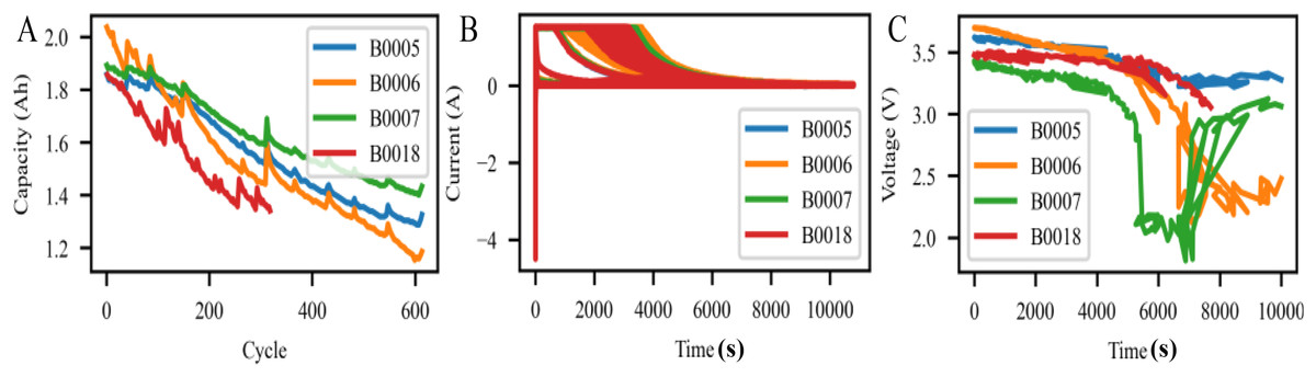
Figure 4: Capacity, current, and voltage variation curves of four lithium-ion batteries (B0005, B0006, B0007, B0018) from the NASA dataset.
Battery performance trends from NASA’s lithium-ion datasets. (A) Capacity degradation over charging cycles for four battery units, showing variation in aging rates. (B) Current profiles during charging/discharging phases over time, illustrating operational dynamics. (C) Voltage curves over time, capturing voltage drop behaviors under different usage patterns.
Evaluation of CNN LSTM attention framework
This section validates the proposed deep learning-based SOH prediction system for lithium-ion batteries using the NASA dataset. As outlined in the workflow (Results), data preprocessing, augmentation, and partitioning were key steps to ensure robust evaluation. To enhance dataset diversity, data augmentation methods—including linear interpolation, cross-enhancement, flipping, and slicing—were applied. The dataset was partitioned into training, validation, and test sets, with flexible parameter control to enable different experimental setups.
Validation sets were dynamically generated through K-fold cross-validation (k = 3), and the independent test set was reserved exclusively for final performance evaluation. These rigorous methodologies ensured unbiased and reliable assessment of the model’s predictive capabilities, as presented in the following results.
It is important to note that, unless explicitly stated otherwise (e.g., the baseline model), all experimental configurations integrate UGABO, MSAWH Loss, and MPC. These core components are fundamental to the system’s design and will not be reiterated in subsequent sections.
As illustrated in Fig. 5, the proposed CNN-LSTM-Attention model was trained and tested on datasets generated by four distinct data augmentation techniques: linear interpolation, cross-validation sampling, flipping, and slicing. Across all four scenarios, the predicted capacity trajectories (in red) closely match the actual measured values (in blue), indicating high consistency in capturing the underlying degradation patterns.
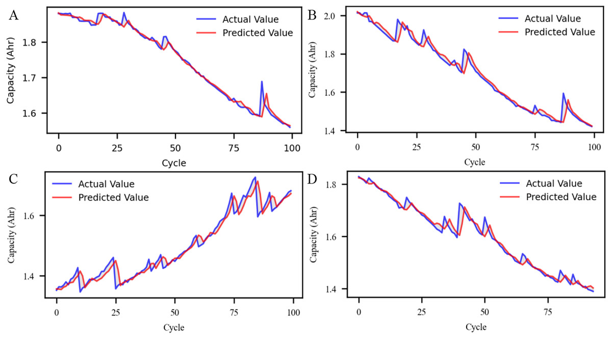
Figure 5: State-of-health (SOH) prediction results under four data augmentation strategies using the proposed deep learning model.
The SOH change curves under four different data augmentation strategies. (A) Shows linear interpolation applied between available data points; (B) represents SOH variation using cross-validation partitioning; (C) depicts results under the flipping method; and (D) illustrates the slicing strategy that segments the cycle data for augmentation. The curves demonstrate how each strategy affects the data trend and smoothness of the SOH trajectory.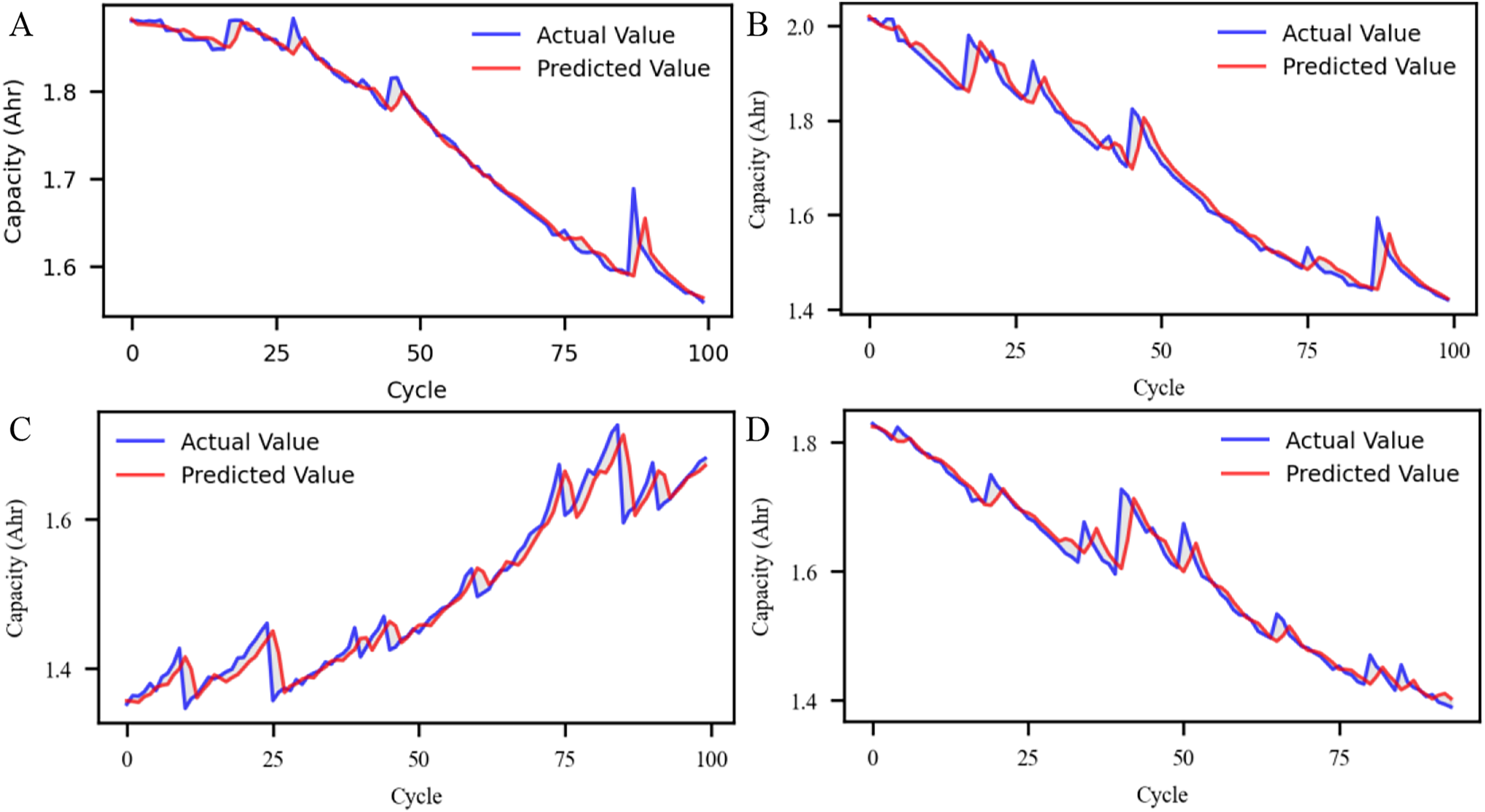
The results demonstrate that the integration of multiple data augmentation techniques significantly enhances the model’s adaptability to diverse input patterns and strengthens its resilience against noise and distributional shifts.
Discussion
Analysis and comparison of different LIB capacity prediction models
This section examines the strengths and weaknesses of different capacity prediction methods. The accuracy of models such as CNN-LSTM-Attention, CNN-GRU-Attention, CNN-GRU, CNN, CNN-LSTM, LSTM, and LSTM-Attention is evaluated. The method resembles that described in ‘Analysis and Comparison of different Hyperparameter Optimization Method’, with the forecast results illustrated in Fig. 6.
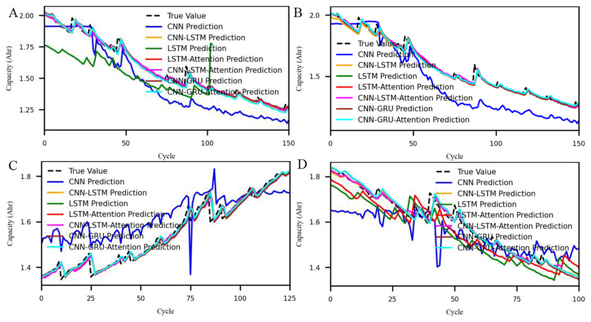
Figure 6: Capacity variation curves across different approaches.
The actual battery capacity against the predicted capacity values across eight deep learning architectures. Each subfigure (A–D) presents results on one battery cell using different models including CNN, LSTM, GRU, and their variants enhanced with attention or hybridized structures. The alignment or deviation of predicted curves from the ground truth highlights the comparative prediction performance of each method.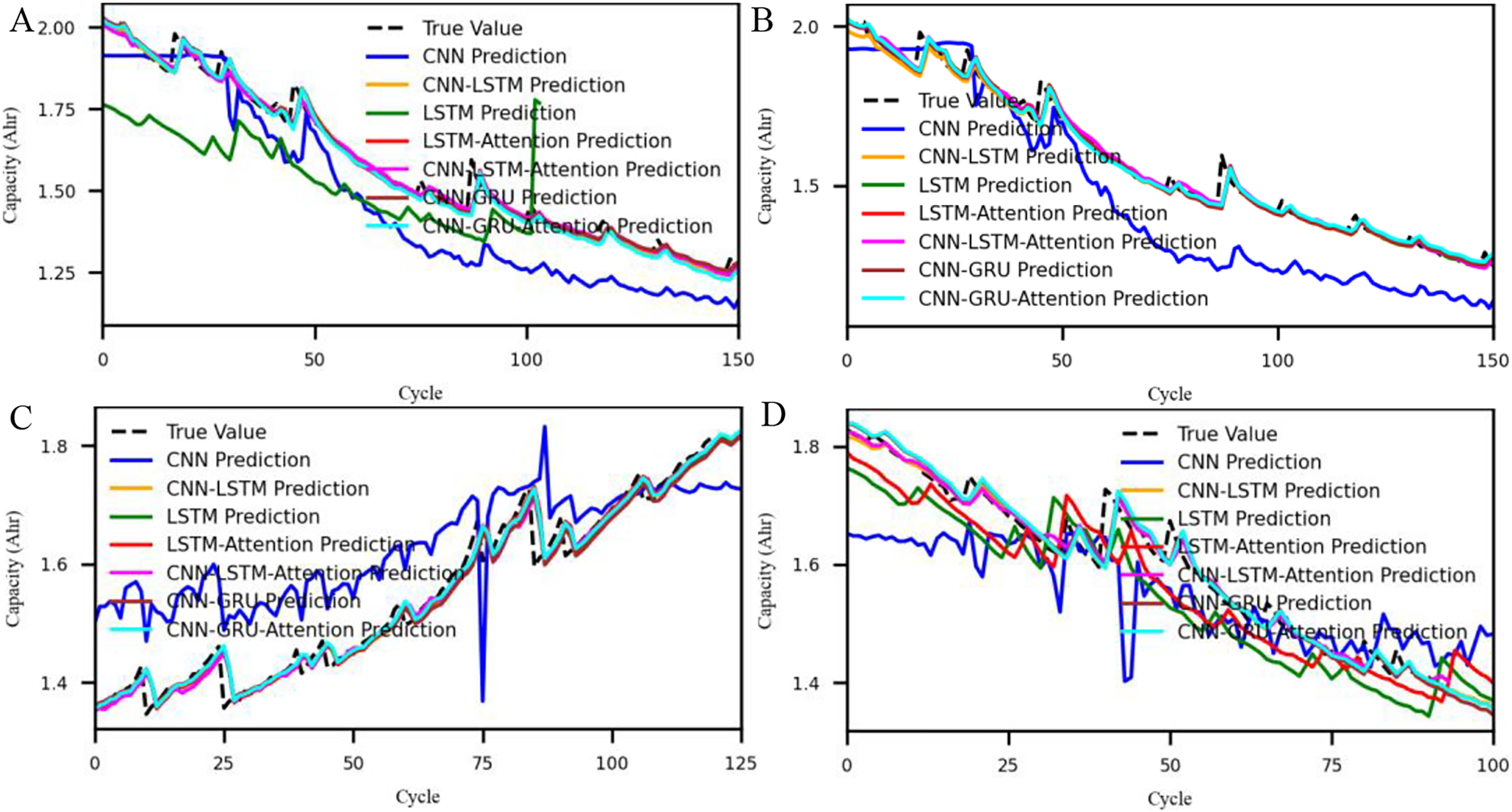
As illustrated in Fig. 6 (capacity trend comparison), multiple deep learning architectures such as CNN-GRU-Attention and CNN-LSTM-Attention demonstrate satisfactory capacity prediction performance. However, a comparative analysis across all seven architectures indicates that CNN performs relatively poorly. Although CNNs are well-suited for capturing spatial patterns, their ability to model temporal dependencies in sequential battery data is limited, making them less effective in SOH estimation tasks. Similarly, while LSTM captures temporal dependencies, its standalone performance is slightly lower, likely due to limitations in feature extraction from raw multivariate inputs. Although certain parameters of CNN-GRU-Attention occasionally outperform those of CNN-LSTM-Attention, the latter exhibits overall smaller prediction errors and superior robustness across different evaluation scenarios. Therefore, we ultimately selected the CNN-LSTM-Attention method for subsequent model development and validation.
Analysis and comparison of different hyperparameter optimization method
In the hyperparameter optimization comparison experiments, the proposed UGABO optimization algorithm was compared with Random Search, Tree-structured Parzen Estimator (TPE), Particle Swarm Optimization (PSO), and Bayesian Optimization under the same model structure. As shown in Fig. 7, the proposed UGABO algorithm consistently outperforms other mainstream hyperparameter optimization methods—including Bayesian Optimization, PSO, Random Search, and TPE—across various data augmentation strategies (interpolation, flipping, slicing, crossover). The box plot in Fig. 7 illustrates that UGABO achieves the narrowest error distribution and the lowest median MAE and RMSE values, reflecting both accuracy and robustness.
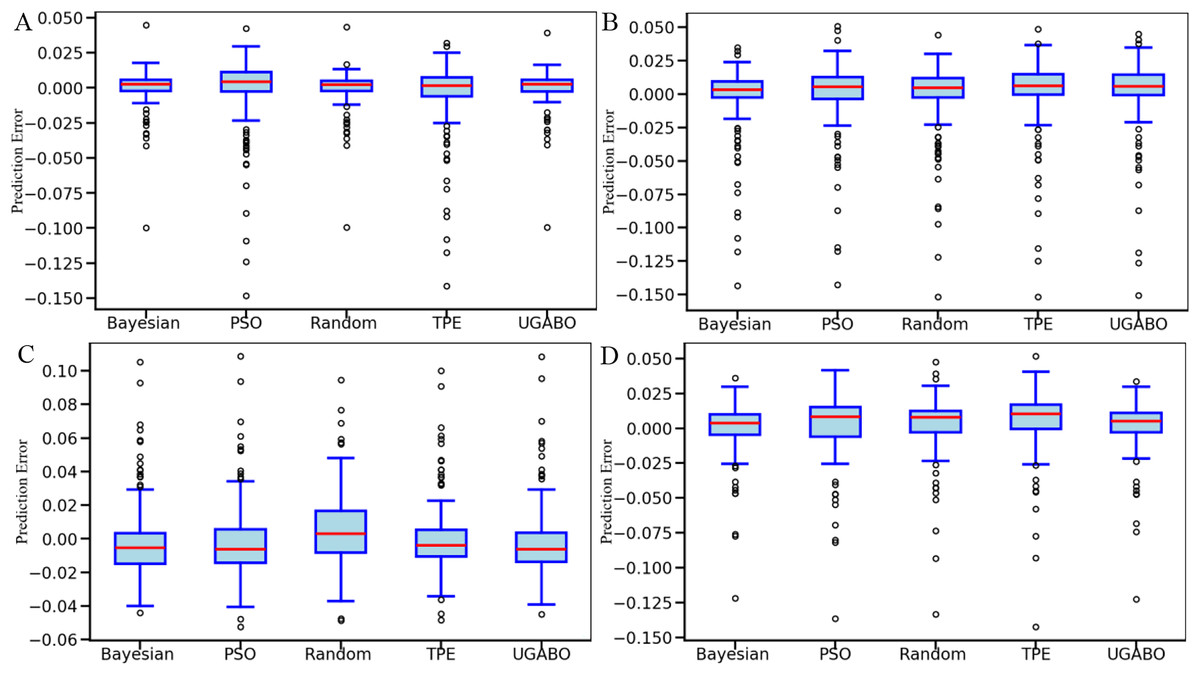
Figure 7: Comparison of prediction error distributions under five hyperparameter optimization methods across four data augmentation strategies.
The prediction errors of five hyperparameter optimization strategies: Bayesian optimization, PSO, Random Search, TPE, and UGABO. Each subfigure (A–D) displays the prediction error distribution on different battery test samples. The center red line represents the median, box edges indicate interquartile ranges, and dots represent outliers. The UGABO method shows superior stability and narrower error dispersion across all tests.
Overall, these results validate that UGABO not only improves model generalization but also offers stable convergence and stronger resistance to noise in high-dimensional search spaces. The consistent dominance of UGABO across multiple metrics and datasets reinforces its practical utility in optimizing deep learning-based SOH prediction models.
Comparison with various loss functions
In this section, the proposed MSAWH Loss, based on the Wasserstein distance, is compared with Huber Loss, Log-Cosh Loss, Mean Squared Logarithmic Error (MSLE), and Smooth L1 Loss. The evaluation metrics used for comparison include R2, MSE, and RMSE. The results are presented in Fig. 8. The testing conditions are similar to those described in ‘Analysis and comparison of different hyperparameter optimization methods’, with the only difference being the type of loss function used in the same model architecture.
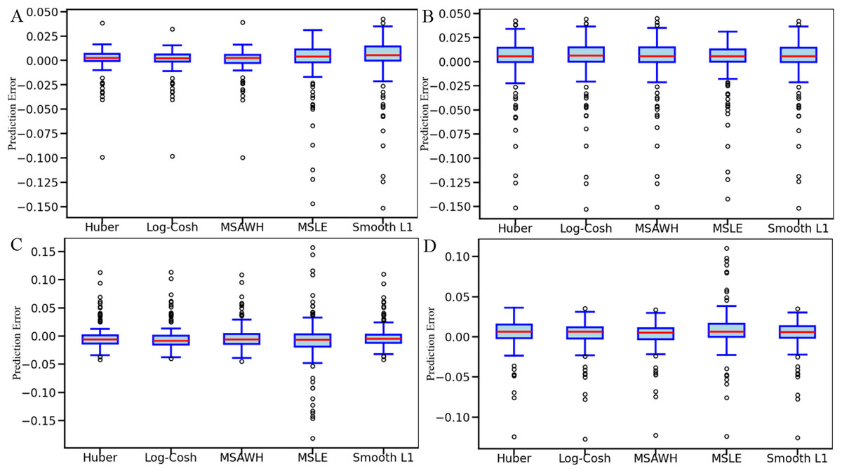
Figure 8: Box plot comparison of prediction errors under different loss functions across four data augmentation methods.
The prediction errors obtained using five different loss functions: Huber, Log-Cosh, MSAWH, MSLE, and Smooth L1. Each subfigure (A–D) corresponds to a battery sample, showing how different loss functions influence prediction accuracy. The MSAWH loss function generally yields lower error distributions, demonstrating its robustness for lithium-ion battery SOH prediction.
As shown in the box plot of Fig. 8, the MSAWH loss function results in a narrower interquartile range and fewer outliers compared to other methods, indicating more stable and reliable predictions.
These trends confirm that MSAWH is not only robust to noisy data but also maintains generalization across different data distributions.
The prediction errors are concentrated within a smaller range, demonstrating that the model exhibits strong robustness in most cases.
Therefore, the integration of multi-scale Wasserstein distance with Huber loss proves particularly effective in handling battery degradation variability and mitigating the influence of abnormal values or distribution shifts.
Evaluation of ablation experiments
This section primarily employs ablation experiments to validate the importance of each component, ensuring the model’s robustness. The experiments are divided into five groups:
(1) Baseline Model: A CNN-LSTM-Attention model that does not utilize UGABO optimization, MSAWH Loss, or MPC error correction. It employs fixed hyperparameters without any hyperparameter optimization methods and uses the Huber Loss function with no error correction algorithm.
(2) Complete model.
(3) Removal of UGABO Hyperparameter Optimization.
(4) Removal of MSAWH Loss Function.
(5) Removal of MPC Error Correction Algorithm.
From Tables 3 to 6, the results indicate that removing any of the three proposed components—UGABO, MSAWH, or MPC—leads to a noticeable degradation in model performance, as reflected by metrics such as MAE and RMSE. Specifically, excluding UGABO results in the highest increase in prediction errors, underscoring its critical role in guiding efficient hyperparameter optimization. Omitting MSAWH widens the error distribution and increases the number of outliers, demonstrating its importance in enhancing error tolerance and mitigating the impact of anomalous data. Likewise, eliminating the MPC module introduces significant fluctuations in the predicted sequences, revealing its effectiveness in smoothing temporal predictions and reducing cumulative error propagation.
| Index | MAE | MSE | MAPE | RMSE | R2 | CRMSD | MAD | nRMSE |
|---|---|---|---|---|---|---|---|---|
| Baseline model | 0.01684 | 0.00076 | 0.01087 | 0.02752 | 0.98757 | 0.24734 | 0.21432 | 0.03200 |
| Complete model | 0.00685 | 0.00016 | 0.00413 | 0.01250 | 0.99333 | 0.15293 | 0.13674 | 0.02733 |
| Remove UGABO | 0.01591 | 0.00073 | 0.00968 | 0.02703 | 0.98690 | 0.23735 | 0.20722 | 0.03345 |
| Remove MSAWH | 0.02524 | 0.00105 | 0.01574 | 0.03234 | 0.98126 | 0.23249 | 0.20440 | 0.04001 |
| Remove MPC | 0.02609 | 0.00134 | 0.01689 | 0.03528 | 0.97811 | 0.26194 | 0.22850 | 0.04102 |
| Index | MAE | MSE | MAPE | RMSE | R2 | CRMSD | MAD | nRMSE |
|---|---|---|---|---|---|---|---|---|
| Baseline model | 0.015340 | 0.00071 | 0.00974 | 0.02667 | 0.98835 | 0.24381 | 0.21114 | 0.03101 |
| Complete model | 0.01489 | 0.00067 | 0.00908 | 0.02583 | 0.98806 | 0.23720 | 0.20734 | 0.03195 |
| Remove UGABO | 0.02126 | 0.00103 | 0.01340 | 0.03157 | 0.98152 | 0.23532 | 0.20397 | 0.03906 |
| Remove MSAWH | 0.02508 | 0.00104 | 0.01564 | 0.03221 | 0.98137 | 0.23255 | 0.20446 | 0.03985 |
| Remove MPC | 0.02353 | 0.00109 | 0.01486 | 0.03287 | 0.98213 | 0.25963 | 0.22434 | 0.03822 |
| Index | MAE | MSE | MAPE | RMSE | R2 | CRMSD | MAD | nRMSE |
|---|---|---|---|---|---|---|---|---|
| Baseline model | 0.01682 | 0.00060 | 0.01087 | 0.02442 | 0.97460 | 0.15056 | 0.13580 | 0.04780 |
| Complete model | 0.01654 | 0.00060 | 0.01080 | 0.02441 | 0.96850 | 0.13573 | 0.12253 | 0.05238 |
| Remove UGABO | 0.01834 | 0.00068 | 0.01197 | 0.02606 | 0.96389 | 0.14044 | 0.12667 | 0.05594 |
| Remove MSAWH | 0.02173 | 0.00067 | 0.01413 | 0.02579 | 0.96485 | 0.13990 | 0.12592 | 0.05535 |
| Remove MPC | 0.01818 | 0.00061 | 0.01175 | 0.02464 | 0.97414 | 0.15098 | 0.13722 | 0.04843 |
| Index | MAE | MSE | MAPE | RMSE | R2 | CRMSD | MAD | nRMSE |
|---|---|---|---|---|---|---|---|---|
| Baseline model | 0.01710 | 0.00069 | 0.01077 | 0.02615 | 0.96368 | 0.13535 | 0.11875 | 0.05511 |
| Complete model | 0.01424 | 0.00051 | 0.00888 | 0.02253 | 0.96938 | 0.12643 | 0.10910 | 0.05130 |
| Remove UGABO | 0.01911 | 0.00080 | 0.01169 | 0.02794 | 0.95166 | 0.13265 | 0.11529 | 0.06363 |
| Remove MSAWH | 0.02368 | 0.00083 | 0.01457 | 0.02874 | 0.95014 | 0.12642 | 0.10978 | 0.06549 |
| Remove MPC | 0.02117 | 0.00089 | 0.01313 | 0.02958 | 0.95249 | 0.14352 | 0.12455 | 0.06237 |
Compared to the baseline model, the improved model achieves a reduction in MAE from 0.01653 to 0.01313 and RMSE from 0.02619 to 0.02132, representing decreases of 20.6% and 18.6%, respectively. Additionally, the average R2 improves from 0.97855 to 0.9798, marking a relative increase of 0.1%, which further validates the effectiveness of the proposed enhancements.
Conclusions
This study introduces a method for analysing lithium-ion battery capacity changes and predicting related parameters using deep learning. The feasibility of the proposed system was confirmed using relevant databases. The main conclusions of this study are as follows:
(1) A novel deep learning architecture was developed to monitor the degradation of battery capacity. Through advanced data preprocessing and network optimization, the proposed framework achieved substantial improvements in prediction performance. Compared with the baseline model, the enhanced system reduced the average MAE and RMSE from 0.01653 and 0.02619 to 0.01313 and 0.02132, respectively. The average R2 value also increased from 0.97855 to 0.9798, indicating enhanced reliability and accuracy.
(2) The integration of four complementary data augmentation techniques, including linear interpolation, slicing, flipping, and cross-validation sampling, significantly improved the diversity and generalization capacity of the training datasets. This enhancement contributed to higher model stability and prediction accuracy.
(3) The proposed UGABO algorithm demonstrated superior effectiveness in hyperparameter tuning. It consistently delivered lower prediction errors and a more concentrated error distribution, indicating strong model stability under various training conditions.
(4) The MSAWH Loss (MSAWH Loss) function outperformed other conventional loss functions by providing more accurate and consistent predictions. Its design allowed the model to respond effectively to errors of varying magnitudes, improving robustness against noise and distributional variation.
(5) The inclusion of the MPC algorithm served as a critical error correction strategy, reducing cumulative prediction errors and ensuring smooth output trajectories. This improvement enhanced the practical reliability of the model under real-world constraints such as voltage, current, and temperature limits.
(6) Ablation studies confirmed that the integrated use of UGABO, MSAWH Loss, and MPC played a pivotal role in enhancing the overall model performance. Each component contributed to more accurate SOH estimation, reinforcing the framework’s effectiveness across multiple evaluation metrics.
Although the proposed method significantly improves prediction accuracy and robustness, several challenges remain. The UGABO algorithm, while effective, imposes high computational costs that may hinder real-time application. Similarly, the MSAWH loss function may be overly sensitive to outliers, and the MPC algorithm’s complexity and resource demands can create performance bottlenecks. To address these issues, future work will focus on enhancing model adaptability by incorporating real-time battery data and accounting for environmental and chemical variability. Variants of UGABO and MSAWH will also be explored to improve performance under practical conditions and broaden real-world applicability.
Supplemental Information
Quantitative comparison of capacity prediction performance using different data augmentation techniques for lithium-ion batteries.
A comparative analysis of four data augmentation strategies—linear interpolation, cross-validation sampling, sequence flipping, and slicing—applied to the task of lithium-ion battery capacity prediction using a deep learning framework. These augmentation techniques aim to enrich the training dataset, improve model generalization, and mitigate overfitting by increasing input diversity and simulating realistic operational scenarios.
Each method was evaluated using eight performance metrics: Mean Absolute Error (MAE), Mean Squared Error (MSE), Mean Absolute Percentage Error (MAPE), Root Mean Square Error (RMSE), R-squared (R²), Centered Root Mean Square Deviation (CRMSD), Median Absolute Deviation (MAD), and Normalized RMSE (nRMSE). These metrics collectively assess predictive accuracy, stability, variance control, and robustness to data irregularities.
Among all augmentation techniques, linear interpolation achieved the best results overall, with the lowest RMSE (0.0125), highest R² (0.9933), and smallest nRMSE (0.0273), demonstrating its effectiveness in generating smooth, consistent synthetic data samples. In contrast, cross-validation sampling exhibited the highest RMSE (0.0258) and nRMSE (0.0319), likely due to discontinuities introduced during stratified resampling. Flipping and slicing methods provided intermediate performance, with slicing outperforming flipping in all evaluated metrics. These results underscore the importance of selecting augmentation methods that align with the temporal dynamics and structure of battery degradation patterns for improved State of Health (SOH) prediction.
Comparative evaluation of hyperparameter optimization algorithms for capacity prediction under linear interpolation-augmented lithium-ion battery data.
A comprehensive comparison of five hyperparameter optimization algorithms—Uncertainty-Guided Adaptive Bayesian Optimization (UGABO), Bayesian Optimization, Particle Swarm Optimization (PSO), Random Search, and Tree-structured Parzen Estimator (TPE)—applied to a CNN-LSTM-Attention model for lithium-ion battery State-of-Health (SOH) prediction. The training data was preprocessed using linear interpolation to augment the original dataset. Performance evaluation is conducted using eight quantitative metrics: Mean Absolute Error (MAE), Mean Squared Error (MSE), Mean Absolute Percentage Error (MAPE), Root Mean Square Error (RMSE), Coefficient of Determination (R2), Centered Root Mean Square Deviation (CRMSD), Median Absolute Deviation (MAD), and Normalized Root Mean Square Error (nRMSE).
Among the compared methods, the proposed UGABO algorithm achieves the best overall performance, with the lowest MAE (0.0068), RMSE (0.0125), and nRMSE (0.0273), and the highest R2 value (0.9933), indicating superior predictive accuracy, model stability, and robustness against noise and overfitting. Traditional methods such as PSO and TPE show relatively higher errors and variability, underscoring the effectiveness of UGABO in navigating high-dimensional, noisy parameter spaces. All evaluations were conducted under consistent training conditions and cross-validation settings to ensure fairness and reproducibility.
Comparative evaluation of hyperparameter optimization methods for capacity prediction based on cross-validation-augmented lithium-ion battery data.
A quantitative comparison of five hyperparameter optimization methods—Uncertainty-Guided Adaptive Bayesian Optimization (UGABO), Bayesian Optimization, Particle Swarm Optimization (PSO), Random Search, and Tree-structured Parzen Estimator (TPE)—for enhancing the performance of the CNN-LSTM-Attention model in predicting the capacity of lithium-ion batteries. The dataset used in this evaluation was augmented using cross-validation slicing to improve the diversity and robustness of the training samples.
The predictive performance of each method was evaluated using eight regression-based metrics: Mean Absolute Error (MAE), Mean Squared Error (MSE), Mean Absolute Percentage Error (MAPE), Root Mean Square Error (RMSE), Coefficient of Determination (R2), Centered Root Mean Square Deviation (CRMSD), Median Absolute Deviation (MAD), and Normalized RMSE (nRMSE).
Results show that the proposed UGABO algorithm achieves the best overall performance, exhibiting the lowest errors across most metrics—e.g., MAE = 0.0148, RMSE = 0.0258, nRMSE = 0.0319—and the highest R2 (0.9880), indicating superior optimization capacity in complex, high-dimensional parameter spaces. In contrast, traditional methods such as PSO and Random Search demonstrate higher variability and less stable convergence, underscoring the advantages of uncertainty-guided adaptive strategies in model calibration. All experiments were conducted under consistent network structures and training conditions to ensure the fairness of comparison.
Comparative evaluation of optimization algorithms for lithium-ion battery capacity prediction using slicing-based data augmentation.
A detailed performance comparison of five hyperparameter optimization algorithms—Uncertainty-Guided Adaptive Bayesian Optimization (UGABO), Bayesian Optimization, Particle Swarm Optimization (PSO), Random Search, and Tree-structured Parzen Estimator (TPE)—applied to the CNN-LSTM-Attention model for lithium-ion battery State of Health (SOH) prediction. All experiments were conducted using datasets augmented by slicing-based techniques, which segment continuous time-series data into fixed-length subsequences. This augmentation strategy increases sample diversity and facilitates localized pattern learning while preserving the temporal coherence of original battery signals.
Performance was evaluated using eight metrics: Mean Absolute Error (MAE), Mean Squared Error (MSE), Mean Absolute Percentage Error (MAPE), Root Mean Square Error (RMSE), R-squared (R²), Centered Root Mean Square Deviation (CRMSD), Median Absolute Deviation (MAD), and Normalized RMSE (nRMSE). These indicators reflect both absolute and relative model accuracy, error stability, and generalization capability.
UGABO consistently outperformed other methods, achieving the lowest RMSE (0.0225) and the highest R2 (0.9693), indicating superior adaptability and predictive precision in the context of data sliced at the sequence level. In contrast, PSO and TPE exhibited relatively higher prediction errors and lower stability, as evidenced by their elevated nRMSE and CRMSD scores. These findings reinforce the advantage of uncertainty-guided adaptive search in navigating complex, high-dimensional hyperparameter spaces, particularly when applied to deep models trained on enriched battery datasets.
Comparative evaluation of optimization algorithms for lithium-ion battery capacity prediction using flipping-based data augmentation.
The performance of five hyperparameter optimization methods—Uncertainty-Guided Adaptive Bayesian Optimization (UGABO), Bayesian Optimization, Particle Swarm Optimization (PSO), Random Search, and Tree-structured Parzen Estimator (TPE)—in the context of predicting lithium-ion battery capacity under a data augmentation strategy based on time-series flipping. Flipping reverses the order of sequences in the training data, thereby improving model generalization by simulating alternate temporal dynamics without altering the data distribution.
Each method was applied to the CNN-LSTM-Attention model architecture under identical network and training conditions. The evaluation was performed using eight quantitative metrics: Mean Absolute Error (MAE), Mean Squared Error (MSE), Mean Absolute Percentage Error (MAPE), Root Mean Square Error (RMSE), Coefficient of Determination (R2), Centered Root Mean Square Deviation (CRMSD), Median Absolute Deviation (MAD), and Normalized RMSE (nRMSE).
Among all tested algorithms, UGABO achieved the most favorable performance across the majority of evaluation metrics, e.g., MAE = 0.0165, RMSE = 0.0244, and R2 = 0.9685, indicating higher prediction accuracy and generalization capability in noise-augmented time-series scenarios. In contrast, PSO showed relatively poorer performance with elevated RMSE (0.0260) and lower R2 (0.9641), highlighting its limited adaptability under augmented training conditions. These results validate the robustness of UGABO in optimizing deep learning models trained with non-standard data transformations.
Comparative analysis of loss functions for lithium-ion battery capacity prediction using linear interpolation data augmentation.
The evaluation results of five loss functions—MSAWH (Multi-Scale Adaptive Wasserstein-Huber), Huber, Log-cosh, MSLE (Mean Squared Logarithmic Error), and Smooth L1—applied to the lithium-ion battery capacity prediction task under a linear interpolation-based data augmentation strategy. Eight statistical performance metrics are used: Mean Absolute Error (MAE), Mean Squared Error (MSE), Mean Absolute Percentage Error (MAPE), Root Mean Square Error (RMSE), Coefficient of Determination (R2), Centered Root Mean Square Deviation (CRMSD), Median Absolute Deviation (MAD), and Normalized Root Mean Square Error (nRMSE). The MSAWH loss demonstrates superior overall performance, achieving the lowest error values in nearly all metrics, notably yielding an MAE of 0.0068 and RMSE of 0.0125, with an R2 of 0.9933. These results indicate that the proposed MSAWH function is more effective at capturing complex degradation patterns and reducing prediction variance. All models were evaluated using 10-fold cross-validation on augmented datasets generated via linear interpolation to ensure reliability and generalization across different data distributions.
Comparative analysis of loss functions for lithium-ion battery capacity prediction using cross-validation data augmentation.
A comparative evaluation of six different loss functions—MSAWH (Multi-Scale Adaptive Wasserstein-Huber), Huber, Log-cosh, MSLE (Mean Squared Logarithmic Error), and Smooth L1—for lithium-ion battery capacity prediction. The performance is assessed across eight widely used regression metrics: Mean Absolute Error (MAE), Mean Squared Error (MSE), Mean Absolute Percentage Error (MAPE), Root Mean Square Error (RMSE), R-squared (R2), Centered Root Mean Square Deviation (CRMSD), Median Absolute Deviation (MAD), and Normalized RMSE (nRMSE). Lower values indicate better performance for all metrics except R2, where a higher value signifies superior model fit. The best performance in each column is highlighted in bold. All results are derived from a 10-fold cross-validation scheme based on augmented datasets to ensure robustness across varying data distributions. This analysis confirms that the proposed MSAWH loss function consistently achieves lower prediction errors and greater robustness, outperforming conventional loss functions in most metrics.
Performance comparison of loss functions for lithium-ion battery capacity prediction using slicing-based data augmentation.
A comprehensive evaluation of six representative loss functions applied to lithium-ion battery State of Health (SOH) capacity prediction under a slicing-based data augmentation strategy. The tested loss functions include: Multi-Scale Adaptive Wasserstein-Huber Loss (MSAW-H), Huber Loss, Log-Cosh Loss, Mean Squared Logarithmic Error (MSLE), and Smooth L1 Loss. Slicing-based augmentation segments long time-series data into fixed-length overlapping subsequences, enhancing the temporal diversity of the training set while preserving meaningful degradation patterns across shorter input windows.
Model performance is assessed using eight quantitative metrics: Mean Absolute Error (MAE), Mean Squared Error (MSE), Mean Absolute Percentage Error (MAPE), Root Mean Square Error (RMSE), R-squared (R2), Centered Root Mean Square Deviation (CRMSD), Median Absolute Deviation (MAD), and Normalized RMSE (nRMSE). These metrics reflect different aspects of predictive performance, including accuracy, variance sensitivity, and robustness to noise.
Among all tested loss functions, MSAW-H achieved the best overall performance, with the lowest RMSE (0.0225), the highest R2 (0.9693), and the lowest nRMSE (0.0513). These results indicate strong model generalization and adaptability to variation-rich, sliced input data. By contrast, MSLE exhibited the highest prediction errors and weakest robustness, likely due to its logarithmic sensitivity, which may amplify noise in non-monotonic short-range subsequences. These findings highlight the importance of selecting loss functions that align with the data augmentation strategy to maximize estimation precision and robustness in SOH modeling.
Performance comparison of loss functions for lithium-ion battery capacity prediction using flipping-based data augmentation.
A comprehensive evaluation of six representative loss functions applied to lithium-ion battery State of Health (SOH) capacity prediction under a flipping-based data augmentation strategy. The tested loss functions include: Multi-Scale Adaptive Wasserstein-Huber Loss (MSAW-H), Huber Loss, Log-Cosh Loss, Mean Squared Logarithmic Error (MSLE), and Smooth L1 Loss. Flipping-based augmentation reverses the sequence of charging/discharging cycles to generate synthetic but temporally plausible training samples, thereby improving the diversity and robustness of the dataset.
Model performance is assessed using eight quantitative metrics: Mean Absolute Error (MAE), Mean Squared Error (MSE), Mean Absolute Percentage Error (MAPE), Root Mean Square Error (RMSE), R-squared (R2), Centered Root Mean Square Deviation (CRMSD), Median Absolute Deviation (MAD), and Normalized RMSE (nRMSE). These metrics reflect model accuracy, prediction stability, and robustness to noise.
Among all tested loss functions, MSAW-H demonstrated the best overall performance, achieving the lowest RMSE (0.0244), highest R2 (0.9685), and lowest nRMSE (0.0523), indicating superior adaptability to augmented sequential data with reduced overfitting and improved error control. In contrast, MSLE yielded the highest prediction errors and weakest robustness, suggesting its sensitivity to logarithmic scaling may not be optimal for SOH estimation tasks involving augmented data. The results highlight the importance of selecting an appropriate loss function that is both distribution-aware and robust to sample variability introduced through augmentation.
Supplemental Information 10
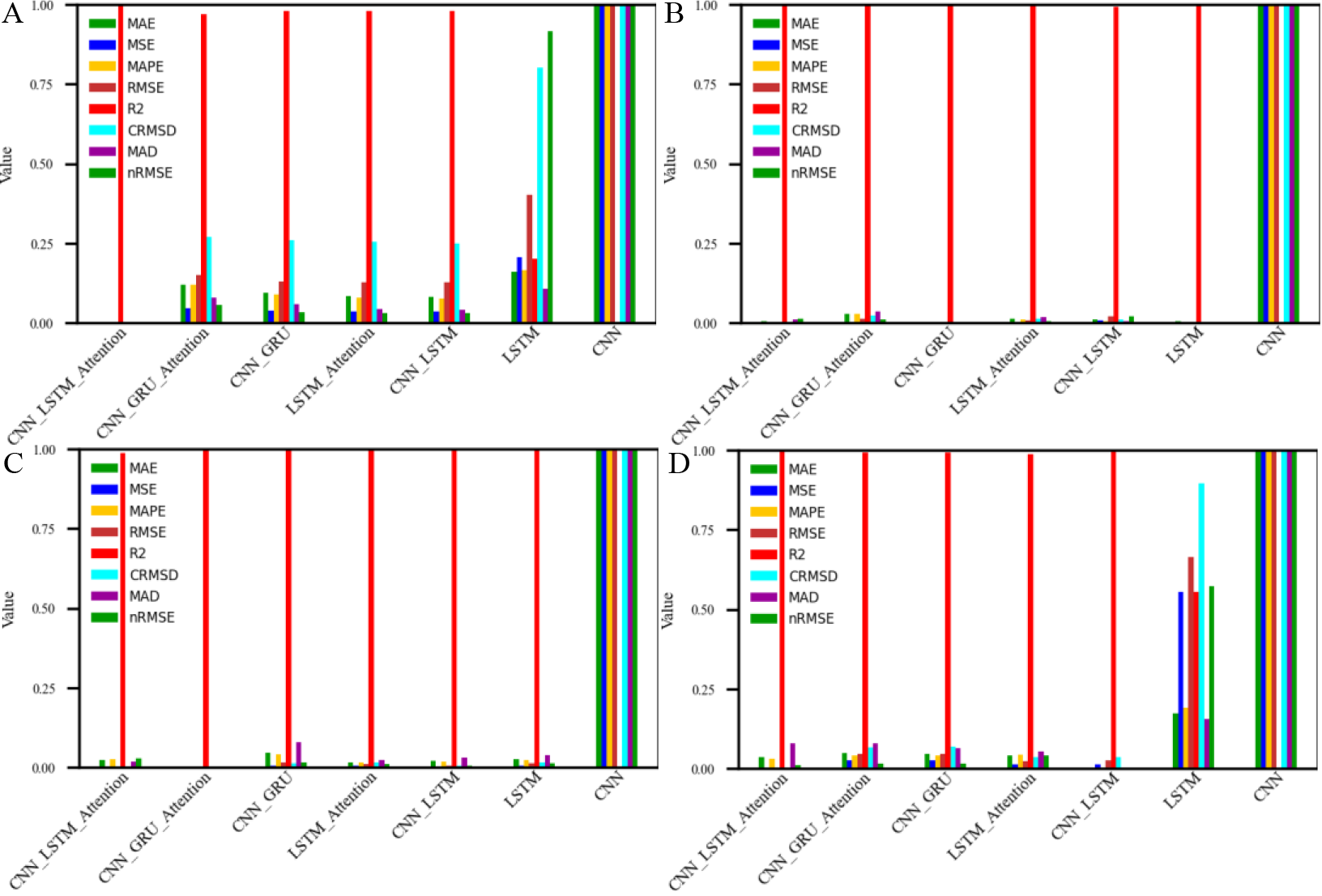
Bar chart comparison of evaluation metrics for different deep learning models under four data augmentation methods.
A comprehensive bar chart comparison of seven deep learning architectures—CNN-LSTM-Attention, CNN-GRU-Attention, CNN-GRU, LSTM-Attention, CNN-LSTM, LSTM, and CNN—evaluated under four distinct data augmentation techniques: (A) linear interpolation, (B) cross-validation sampling, (C) flipping, and (D) slicing. The evaluation is based on eight performance metrics: Mean Absolute Error (MAE), Mean Squared Error (MSE), Mean Absolute Percentage Error (MAPE), Root Mean Square Error (RMSE), R-squared (R2), Centered Root Mean Square Deviation (CRMSD), Median Absolute Deviation (MAD), and Normalized RMSE (nRMSE), as shown in the legend.
Each subplot (A–D) visualizes the performance of the models trained with a specific augmentation method. Taller bars in RMSE and nRMSE generally indicate poorer performance, whereas lower bars in MAE, MSE, and MAPE reflect better accuracy. Higher R2 values, shown in red, correspond to better regression fit.
Across all augmentation techniques, the CNN-LSTM-Attention architecture consistently exhibits superior predictive performance, achieving lower error values and higher stability across most metrics. In contrast, the baseline CNN and LSTM models display greater variability and poorer performance, particularly in RMSE and nRMSE, highlighting the limitations of using single-module architectures for complex sequential battery data. These results emphasize the robustness and adaptability of hybrid attention-based models under diverse data augmentation schemes.
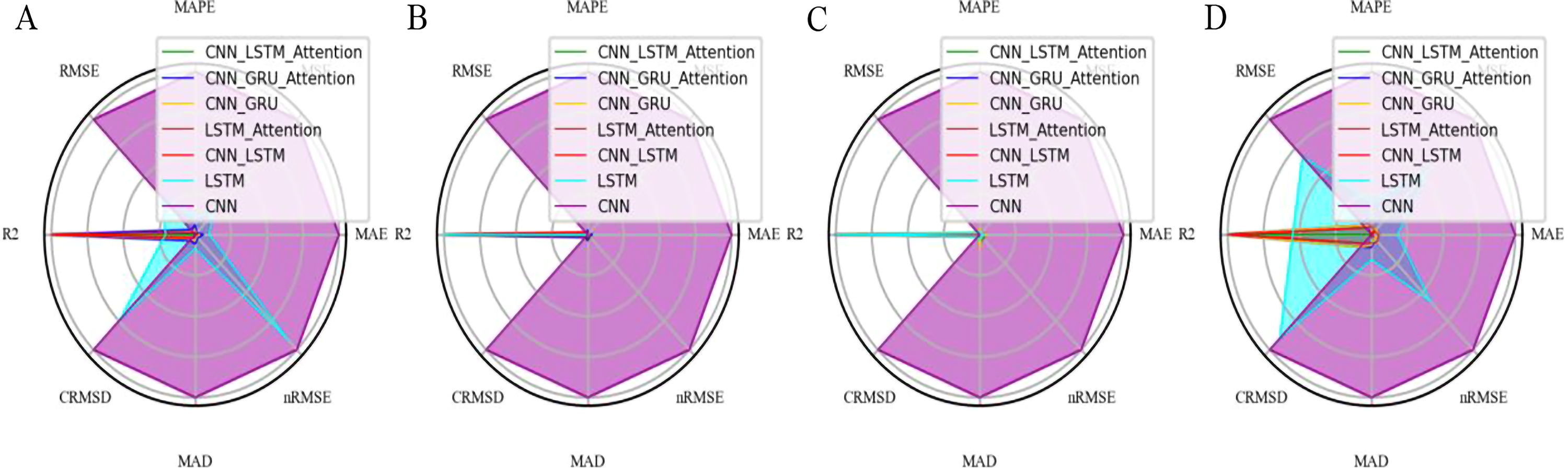
Radar chart comparison of seven model architectures across six evaluation metrics under four data augmentation scenarios.
The comparative performance of seven deep learning architectures—CNN-LSTM-Attention, CNN-GRU-Attention, CNN-GRU, LSTM-Attention, CNN-LSTM, LSTM, and CNN—using radar plots across eight evaluation metrics: Mean Absolute Error (MAE), Mean Squared Error (MSE), Mean Absolute Percentage Error (MAPE), Root Mean Square Error (RMSE), R-squared (R2), Centered Root Mean Square Deviation (CRMSD), Median Absolute Deviation (MAD), and Normalized RMSE (nRMSE). Panels (A) through (D) correspond to four distinct data augmentation techniques: (A) linear interpolation, (B) cross-validation sampling, (C) flipping, and (D) slicing.
The outermost edge of the radar chart indicates poorer performance (higher error or lower R2), while regions closer to the center represent better model behavior. Notably, the CNN-LSTM-Attention model consistently encloses the smallest area across all subplots, indicating superior overall performance in terms of accuracy, robustness, and generalizability under diverse augmentation schemes. In contrast, single-module models such as CNN and LSTM tend to occupy larger outer regions, reflecting less favorable prediction outcomes. These visualizations further reinforce the effectiveness of hybrid attention-based architectures for State of Health (SOH) estimation in lithium-ion batteries.