
Executing native Java code in R: an approach based on a local server
- Published
- Accepted
- Received
- Academic Editor
- Marieke Huisman
- Subject Areas
- Scientific Computing and Simulation, Programming Languages
- Keywords
- Interoperability, Java local server, TCP/IP connection, R vectorization, Java Native Interface
- Licence
- This is an open access article distributed under the terms of the Open Government License.
- Cite this article
- 2020. Executing native Java code in R: an approach based on a local server. PeerJ Computer Science 6:e300 https://doi.org/10.7717/peerj-cs.300
Abstract
The R language is widely used for data analysis. However, it does not allow for complex object-oriented implementation and it tends to be slower than other languages such as Java, C and C++. Consequently, it can be more computationally efficient to run native Java code in R. To do this, there exist at least two approaches. One is based on the Java Native Interface (JNI) and it has been successfully implemented in the rJava package. An alternative approach consists of running a local server in Java and linking it to an R environment through a socket connection. This alternative approach has been implemented in an R package called J4R. This article shows how this approach makes it possible to simplify the calls to Java methods and to integrate the R vectorization. The downside is a loss of performance. However, if the vectorization is used in conjunction with multithreading, this loss of performance can be compensated for.
Introduction
The R language (Venables & Smith, 2020) has gained in popularity over the last decades. It has been recently ranked the tenth most popular language according to the TIOBE index (Tiobe, 2020). This interpreted language was primarily designed for data analysis and statistics (Wickham, 2014, Ch. 16) and it is now widely used by the scientific community.
Some scientific problems, especially those involving modelling, require complex object-oriented implementation and computational performance that can hardly be achieved in R. Object-oriented languages such as C++ and Java are better suited for this task since they allow for encapsulation and polymorphism (Schildt, 2007, Ch. 2). According to different surveys, Java counts among the five most popular languages in computer programming (GitHub, 2018; Stack Overflow, 2018; Tiobe, 2020). Compared to other languages, Java has the advantage of being highly portable thanks to a virtual machine technology. This virtual machine makes the interface between the operating system (OS) and the Java code. In practice, the Java Virtual Machine (JVM) comes with the Java installation package.
In terms of performance, the first versions of Java were considered to be slower than C++. However, the JVM technology has improved over time and the two languages now show a comparable performance in some contexts (Vivanco & Pizzi, 2002; Costanza, Herzeel & Verachtert, 2019), even though it is still widely accepted that C++ is slightly faster than Java. One thing for sure, these two languages are faster than R, mainly because of their implementation (Wickham, 2014, Ch. 16).
When dealing with complex models, invoking native Java or C++ code directly in R can result in a significant gain in computational time compared to translating the code and running it directly in the R environment. This idea of making calls between different languages is referred to as interoperability (Epperly et al., 2012). Interoperability has the major advantage of avoiding code replication across different languages and thereby it decreases the maintenance effort, since only one version of the source code exists.
The basic installation of R already provides tools that can run native C and C++ code. Some statistical packages, such as nlme and lme4, rely on these tools for tedious mathematical operations in order to reduce the computational time (Pinheiro, Bates & R Core Team, 2017; Bates et al., 2019). The rJava package is a low-level R to Java interface that has been available for over a decade (Urbanek, 2020). This package makes it possible to start a JVM embedded in the R environment and to execute native Java code using the well-known Java Native Interface (JNI, see Liang, 1999).
The JNI can be used both ways: it allows running native code within a Java environment or running Java code in a foreign environment. It has been described by some as a powerful tool for linking Java to other environments (Getov, Gray & Sunderam, 2000), while being criticized by others for its complexity (Kondoh & Onodera, 2008; Veerasamy & Nasira, 2012). This complexity has led to the development of simplified interfaces, all derived from the original JNI, such as SafeJNI (Tan et al., 2006) and a JNI–C++ integration (Gabrilovich & Finkelstein, 2000). In R, some packages, such as the jsr223 and jdx packages (Gilbert & Dahl, 2020a, 2020b), build on the JNI-based interface of rJava but offer a simpler interface. Since 2009, the rJava package also implements a high-level interface that facilitates the instantiation of Java objects and the calls to Java methods, but it comes with a significant loss of performance (Dahl, 2020a).
Another option for running native code in a foreign environment consists of creating a distinct environment for each language and making these environments interact through a Transmission Control Protocol/Internet Protocol (TCP/IP) connection (Liang, 1999, p. 6). The py4j library (www.py4j.org), which enables a connection between Java and Python, is an example of this approach. Another example is that of the rscala package (Dahl, 2020a, 2020b) which uses a TCP/IP connection to create a bridge between R and the Scala language.
In the context of native Java code run in R, this approach could be a simpler alternative to the use of the JNI. It would offer a greater flexibility in the execution of the native code, allowing for the on-the-fly conversion of primitive types and the inclusion of R vectorization (De Vries & Meys, 2015, p. 15). Moreover, because the two environments are created in independent processes, it would make the code easier to debug on both ends.
This article shows how this approach was implemented in an R package called J4R. The initial objective of this work was to create a package that
-
Can be easily installed;
-
Keeps the syntax simpler than that of the JNI;
-
Offers a reasonable performance;
-
Takes advantage of some features of R such as the vectorization;
-
Can be debugged on both ends.
Methodology
Package description
Java is a highly structured object-oriented language. Functions and variables are all embedded into the classes. They are usually referred to as methods and fields, respectively. For the sake of clarity, this terminology will be used throughout this paper so that any occurrence of “method” or “field” refers to Java whereas terms “function” and “variable” are related to R.
It is assumed that the reader has a certain knowledge of some concepts related to object-oriented programming and to the Java language in particular, such as class inheritance and field and method modifiers. Should it not be the case, the reader is referred to Schildt (2007).
The main functions of the J4R package are listed in Table 1. Most of them are further described through examples in the following sections. The package implements a series of more than a hundred unitary tests, which have been successfully run with Java versions 8, 11 and 13 on Windows and Linux.
| Function | Purpose |
|---|---|
| connectToJava | Instantiate a local server in Java |
| shutdownJava | Shut down the local server |
| addToClassPath | Dynamically add a path to the class path |
| interruptJava | Interrupt the current task |
| createJavaObject | Create instances, arrays or uninstantiated (null) objects |
| callJavaMethod | Invoke a public method |
| getJavaField | Retrieve the value of a public field |
| setJavaField | Set the value of a public field |
| callJavaGC | Call the garbage collector in R and Java |
| as.JavaArray | Convert R vectors and matrices to Java arrays |
Linking Java and R through a TCP/IP connection
Linking two environments through a TCP/IP connection is very similar to a server replying to the requests from a client application. The only distinction between the two concepts is that the client and the server are both running on the same machine in the first whereas they are located on two different computers in the latter. Practically speaking, the J4R package contains an R client which instantiates a local server in Java (Fig. 1). This server listens to several internal ports. The R client connects to the server through these ports using a socket connection. Once connected, it can send requests to the Java server, which processes them and sends the result back to the client.
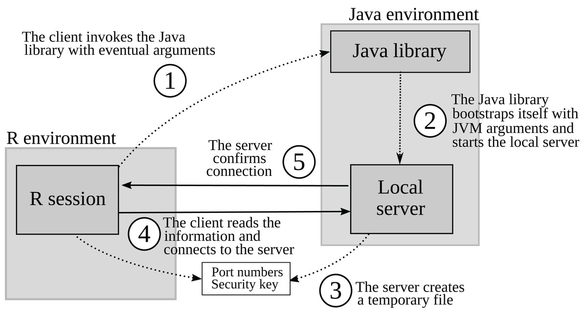
Figure 1: How the J4R package creates a local server in Java and connects to it.
Each numbered circle represents a step in the initialization of the local server.
The J4R package includes a Java library packaged as a runnable jar file. This library (j4r.jar) implements the local server in the following classes:
-
JavaProcess: Instantiate the JVM in an independent process
-
JavaLocalGatewayServer: Implement a local server
-
REnvironment: Translate the requests received from the R client and process them in Java
The R client in the J4R package invokes the Java library using the system2 function (Step 1 in Fig. 1). Additional arguments such as the classpath and the memory size of the JVM can be passed as well. When invoked, the Java library creates a JVM that bootstraps itself using the JavaProcess class and the arguments it received from the R client (Step 2). This results in a second JVM with the appropriate classpath and memory size. An object of the JavaLocalGatewayServer class is then instantiated within this second JVM. The server creates a temporary file containing the different port numbers and a security key in the working directory of the R session (Step 3). The R client retrieves the information from the temporary file and then connects to the server using the appropriate port numbers and the security key (Step 4). Once the R client is connected and the security key has been validated, the server sends confirmation (Step 5).
The first JVM has two main roles: it makes sure the arguments sent by the client conform to the Java syntax and it adds some arguments required for the dynamic classpath definition. In Java, the classpath is handled by instances inheriting from the ClassLoader class (Schildt, 2007, p. 418). There was a major rehauling of these classes between Java 8 and 9 (Kanagalingam, 2019) so that the JVM must be started with specific arguments in the latest versions in order to enable the dynamic classpath. Because these tasks do not require a lot of memory, the first JVM is instantiated by the client with an allocation of 50 Mb.
Once connected to the server, the R client can send requests. Those requests are processed by an instance of the REnvironment class in Java. The result of this processing is sent back to the R client through the same TCP/IP connection. The information sent back and forth through the TCP/IP connection is first translated into character strings and then re-interpreted on the other end. If the connection is severed for some reason, the Java server automatically shuts down, and both JVMs exit so that it leaves no idle process in memory.
In practice, the lasted version of the J4R package can be installed from the SourceForge repository through the following line of code:
> J4Rurl <- “https://sourceforge.net/projects/repiceasource/files/latest”
> install.packages(J4Rurl, repos = NULL, type=“source”)
…
>
Then, the Java server can be instantiated as follows:
> connectToJava()
Starting Java server…
Server started
[1] TRUE
>
Likewise, the Java server can be shut down by calling the shutdownJava function:
> shutdownJava()
Closing connections and removing sockets…
Shutting down application…
Done.
>
By default the server listens to two ports randomly selected among those that are available. It is possible to change the number of ports the server is listening to through the port argument:
> connectToJava(port = 0)
Starting Java server…
Server started
[1] TRUE
>
Since the port argument has a length of one, the server is instantiated with a single listening port. Moreover, since its value is 0, the port is selected at random. The J4R package allows for a maximum of four listening ports. Each successful socket connection to a particular port is handled by an individual thread on the Java end. In the R environment, all the socket connections are handled by a single instance of the connectionHandler class. In addition to these ports, the connectionHandler instance creates two other connections to the server. The first one is a backdoor connection with the Java server. This backdoor connection can be used if an interruption of the native code is required or if the Java server must be abruptly terminated (see Subsection “Interrupting native code”). The other connection is used to synchronize the garbage collection of both environments (see Subsection “Memory management”).
Creating Java objects
The REnvironment class in the j4r Java library heavily relies on the Reflection API available in Java (see Shams & Edwards, 2013) for the instantiation of objects and the call to methods. In J4R, the createJavaObject function makes it possible to
-
instantiate Java objects;
-
instantiate arrays;
-
retrieve uninstantiated objects, that is, objects of particular classes with their value set to null.
Once an object has been created, the Java server stores it in an internal map with its identity hash code acting as a key. In Java, the identity hash code is a quasi-unique integer that is attributed to each object based on its internal address in memory (Marx, 2010). The class of the object and its identity hash code are the two elements that are sent back to the R client as a pointer to the real Java object. Subsequent actions on this object, such as invoking a method of its class or passing it as an argument to the method of another class, is made possible through this pointer.
Upon reception, the R client instantiates an R object of the java.object class, which extends the environment class and has two slots: one for the Java class name and the other for the Java object identity hash code. Whenever this pointer is sent back to the Java server, then the true object is retrieved from the internal map. Because of the fundamental role it plays, this internal map will be referred to as the pointer map. The consequences of this pointer map on the memory management will be addressed later in this section.
The createJavaObject function requires a class name. It also accepts eventual arguments if the constructor of the class requires some. Two additional arguments, isNullObject and isArray, are set to false by default. For the sake of the example, let us focus on the ArrayList class in Java. Let us also assume that the local server is running and that the R client is connected. The instantiation of a Java object of the ArrayList class goes like this:
> myJArrList <- createJavaObject(“java.util.ArrayList”)
> myJArrList
[1] “java.util.ArrayList@2057477420”
>
Since the createJavaObject function was given a single argument in the previous example, namely the class name, the Java server instantiated the object using the empty constructor of the ArrayList class. This same class also includes an alternative constructor that requires an integer to create an ArrayList object with a specific initial capacity. Such an object can be created as follows:
> my2ndJArrList <- createJavaObject(“java.util.ArrayList”,
as.integer(10))
>
Here, the argument passed to the constructor is an integer, which is considered as a primitive type. The server automatically recognizes the class or the primitive type of the argument. Primitive types in R are converted on the fly into Java primitive types (Table 2), with the notable exception of the character type in R that is converted into an object of the String class in Java. Because the communication to and from the server takes the form of character strings, doubles and numerics are converted to an IEEE 754 representation (IEEE, 2008) with 16 decimals. In practice, there is no loss of precision.
| R | Java |
|---|---|
| integer | int |
| character | String |
| numeric | double |
| logical | boolean |
In the previous example, the Java server recognized an integer and looked for the constructor ArrayList(int i). If one omits to cast 10 as an integer, then the Java server recognizes this type as a numeric and it looks for the constructor ArrayList(double d). Since this constructor does not exist, an exception is returned to the R client:
> my3rdJArrList <- createJavaObject(“java.util.ArrayList”, 10)
Error in .checkForExceptionInCallback(callback):
java.lang.NoSuchMethodException: java.util.ArrayList.<init>(double)
>
Arrays and uninstantiated objects can also be created by setting the arguments isArray and isNullObject to true when calling the createJavaObject function. Note that the as.JavaArray function provides a simpler interface for the instantiation of Java arrays.
Invoking Java methods from R
Java methods that are public can be invoked using the callJavaMethod function, which requires at least a source argument and the name of the method to be invoked. Additional arguments passed to the function are assumed to be the arguments of the Java method. When these additional arguments are passed to the function, the Java server automatically retrieves their class or primitive type in order to find the appropriate method through the Reflection API. For example,
> callJavaMethod(myJArrList, “size”)
[1] 0
> callJavaMethod(myJArrList, “add”, 4)
[1] TRUE
> callJavaMethod(myJArrList, “size”)
[1] 1
> callJavaMethod(myJArrList, “get”, as.integer(0))
[1] 4
>
The first call invokes the size method on the ArrayList object we created in a previous example. The method returns 0 to the R client, since the ArrayList object is empty. This value is converted on the fly into an integer by the R client. The second call invokes the add(Object obj) method, which stores the value 4 as a double due to the on-the-fly conversion of numeric into double (Table 2). The third call invokes the size method again, which returns the value 1 this time. Finally, the fourth call retrieves this value just stored in the ArrayList object at index 0. Note: Java indexes the arrays starting from 0 whereas the indexes start from 1 in R.
Invoking static methods through the callJavaMethod function is made possible by setting the source argument to a class name instead of a java.object instance. For example, the Math class contains a static method called sqrt, which computes the square root of a double. This static method can be invoked as follows:
> callJavaMethod(“java.lang.Math”, “sqrt”, 10)
[1] 3.162278
>
Whenever the source is a java.object instance, the $ operator can be used in place of the callJavaMethod function, yielding a syntax that is closer to that of Java. For instance, the four calls to callJavaMethod performed on the myJArrList object in the previous example could be:
> myJArrList$size()
[1] 1
> myJArrList$add(4)
[1] TRUE
> myJArrList$size()
[1] 2
> myJArrList$get(as.integer(0))
[1] 4
>
Accessing and changing public fields
Public fields can be accessed through the getJavaField function which requires two arguments, a source and the field name. The source is either a java.object instance or a class name in the case of a public static field.
The setJavaField function makes it possible to set the value of such fields as long as they are not final. The function requires three arguments, a source, a field name and the value to be set. For the sake of the example, let us consider the following Java class:
public class MyTestClass {
public int i;
public MyTestClass(int i) {
this.i = i;
}
}
If we assume that the binary of this class is in the working directory, an instance can be created as follows:
> addToClassPath(“.”)
> a <- createJavaObject(“MyTestClass”, as.integer(1))
>
Here, the addToClassPath function adds the working directory to the class path so that the MyTestClass class can be loaded. Once the instance has been created, the public field i can then be accessed and changed using the aforementioned functions:
> getJavaField(a, “i”)
[1] 1
> setJavaField(a, “i”, as.integer(10))
> getJavaField(a, “i”)
[1] 10
>
When the source argument is a java.object instance, the $ operator can be substituted for the two functions as in the following lines of codes:
> a$i <- as.integer(1)
> a$i
[1] 1
>
Using the R vectorization with native Java code
A unique feature of R is its ability to perform operations on vectors (De Vries & Meys, 2015, p. 15). In J4R, the createJavaObject, callJavaMethod, getJavaField and setJavaField methods allow for this vectorization. For example, if a vector of integers is passed to the createJavaObject function, many objects of the same class can be created at once:
> myJArrLists <- createJavaObject(“java.util.ArrayList”,
as.integer(rep(10,3)))
> myJArrLists
[1] “[1] java.util.ArrayList@1322605515”
[1] “[2] java.util.ArrayList@1002797593”
[1] “[3] java.util.ArrayList@1525351974”
>
Here, the Java server instantiated three ArrayList objects with an initial capacity of 10. The three pointers to these objects were returned to the R client and embedded into a java.list object. The same applies to the callJavaMethod function:
> callJavaMethod(myJArrLists, “add”, 5)
[1] TRUE TRUE TRUE
> callJavaMethod(myJArrLists, “add”, c(5,7,9))
[1] TRUE TRUE TRUE
> callJavaMethod(myJArrLists[[3]], “get”, as.integer(c(0,1)))
[1] 5 9
>
The first call to the callJavaMethod function adds the value 5 to all three ArrayList objects whereas the second call adds 5, 7, and 9 to the first, second and third ArrayList objects, respectively. The third call just confirms that the values stored in the third ArrayList object are 5 and 9. Inconsistent numbers of elements in the vectors or the eventual java.list objects cause the function to return an error. For instance, if one tries to add 5 and 7 to a java.list object of size 3, then the function returns an error:
> callJavaMethod(myJArrLists, “add”, c(5,7))
Error in .getSourceLength(source, parametersLength):
The length of the java.list object
or the vector is inconsistent with the length of the parameters!
>
Note that the $ operator can be used in place of the callJavaMethod, getJavaField and setJavaField functions when the source argument is a java.list object so that the three calls in the previous example could be re-expressed as:
> myJArrLists$add(5)
[1] TRUE TRUE TRUE
> myJArrLists$add(c(5,7,9))
[1] TRUE TRUE TRUE
> myJArrLists[[3]]$get(as.integer(c(0,1)))
[1] 5 9
>
Since large java.list objects and vectors could exceed the buffer size of the socket connection, the R client breaks down these large sets into smaller sets with a maximum of 200 elements each. These smaller sets are successively sent to the server. The results of these calls are recomposed into a single object by the client.
Creating Java arrays
Since vectors are automatically perceived as an attempt to use R vectorization, any method or constructor involving an array will be misinterpreted. The Java Arrays class provides many static methods to manipulate arrays. The argument of these static method is obviously an array. For example, the sort method makes it possible to sort the values within an array of doubles. Because vectors are not automatically converted into arrays in J4R, the following line of code will inevitably throw an exception:
> callJavaMethod(“java.util.Arrays”, “sort”, c(22,10,14))
Error in .checkForExceptionInCallback(callback) :
java.lang.NoSuchMethodException: Method sort cannot be found in the
class Arrays
>
The array must be instantiated first and then passed to this method. This can be done through the as.JavaArray function of the J4R package. The function returns a pointer to the array instance which can be passed to a method or a constructor as follows:
> myArray <- as.JavaArray(c(22,10,14))
> myArray
[1] “One-dimension array of D@1799180931”
> callJavaMethod(“java.util.Arrays”, “sort”, myArray)
> getAllValuesFromArray(myArray)
[1] 10 14 22
>
The myArray variable is a pointer to an array of doubles. Calling the sort method in Java sorts the values of the array in ascending order. The reconversion to R is obtained through the getAllValuesFromArray function. Note that the as.JavaArray function accepts vectors and matrices of any primitive types listed in Table 2.
Interrupting native code
R is meant to handle the interruption of native code in C and C++ (Wickham, 2015, Ch. 10). To the best of my knowledge, there is no guideline for other languages. J4R implements a workaround that allows for interruption of native Java code. In this example, the thread that handles to code on the Java end is asked to “sleep” for a 100 s:
> callJavaMethod(“java.lang.Thread”, “sleep”, as.long(100000))
Note that the sleep method takes a long as argument. Since this type is not available in R, it must be casted using the as.long function.
Trying to interrupt this code from the R console or R Studio is virtually impossible. A workaround consists of starting a new session and making sure that the working directory points to the same folder than that of the first session. With R Studio, this is done automatically. The J4R package implements a function called interruptJava which connects to the server through the backdoor connection and requests the interruption of all the threads associated with the client. This function relies on the Thread.interrupt method on the Java end.
After opening the second session, the user can enter the following line of code to request an interruption of the native Java code:
> J4R::interruptJava()
>
which results in an InterruptedException in the first session:
> callJavaMethod(“java.lang.Thread”, “sleep”, as.long(100000))
Error in .checkForExceptionInCallback(callback) :
java.lang.InterruptedException: sleep interrupted
>
This interruption mechanism assumes that the Java code is meant to be interrupted.This can be achieved by invoking methods that throw InterruptedException or by periodically invoking the Thread.interrupted method (Oracle, 2019). If the Java code does not invoke these methods, it cannot be interrupted. A successful interruption does not affect the connection to the server. The thread in charge of the connection on the Java end resumes and waits for the next request.
The interruptJava function assumes that the temporary file containing the security key and the port numbers is still available. For this reason, it is strongly recommended to shut down this second session after calling the interruptJava function. Any call to other functions such as connectToJava will instantiate a new Java server and produce a new version of the temporary file. In such a context, the port number of the backdoor socket and the security key associated to the server instantiated in the first session will no longer be available.
Memory management
In Java, instances can be automatically removed from the memory when they are no longer needed. This technique is known as garbage collection (Schildt, 2007, p. 121). When it is called, the garbage collector removes all the objects for which no references exist. This means that these objects are no longer tied to any ongoing tasks.
In the J4R package, the Java server keeps all the instances created through the createJavaObject, callJavaMethod and getJavaField functions in the aforementioned pointer map. This pointer map is part of the REnvironment class. It is created as soon as a new client connects to the server and, as long as the local server is running and the client is connected, a reference to this map exists.
Memory management in R is also based on garbage collection (Wickham, 2014, p. 383). In J4R, the java.object class implements a finalizer that is run when the garbage collection occurs. This finalizer does two things. First, the collected instance is temporarily stored in a java.list instance hidden in the cache environment of the J4R package. This java.list instance acts as a dump pile. Secondly, it checks if the dump pile contains more than a hundred java.object instances. If it does, these pointers are sent to the server through a dedicated connection with the express request to release their associated objects from the pointer map. These objects are then subject to garbage collection in Java. The java.object instances sent to the Java server are removed from the dump pile and they are finally collected by the garbage collector in R.
The J4R package also implements the callJavaGC function which clears the dump pile regardless of the number of java.object instances it contains.
Multithreading
Each connection to a listening port of the Java server is handled by an individual thread. The user can take advantage of this setup to execute Java code on multiple threads when the server is instantiated with two or more listening ports. The four main functions that run native Java code—createJavaObject, callJavaMethod, getJavaField and setJavaField—all have an argument called affinity, which is set to 1 by default. This affinity refers to the connection port and thereby to a particular thread on the Java end.
Multithreading in R is made possible through several packages, such as parallel (R Core Team, 2020) and snow (Tierney et al., 2018). The J4R package implements a function called mclapply.j4r which is a wrapper for the original mclapply function of the parallel package. The mclapply.j4r function requires two arguments: a vector of numerics and a function that is to be executed in different threads. This special function must have two arguments: the first stands for the individual numerics that compose the vector whereas the second argument defines the affinity to a particular port of the Java server. This two-argument function executes the Java code by calling the createJavaObject, callJavaMethod, getJavaField, or setJavaField functions. The affinity argument must be specified in each call to these four functions. A simple example is:
> if (getNbConnections() == 1) {
+ shutdownJava()
+ connectToJava()
+ }
Closing connections and removing sockets…
Shutting down application…
Done.
Starting Java server…
Server started
[1] TRUE
> f <- function(i, aff) {
+ myArrayList <- createJavaObject(“java.util.ArrayList”,
+ affinity = aff)
+ callJavaMethod(myArrayList, “add”, 5, affinity = aff)
+ }
> result <- mclapply.j4r(1:1000, f)
>
So far, we had been running the server with a single listening port. The first condition shuts down the server and restarts it with two listening ports. Then, the function f is defined and processed a thousand times. At each call, a Java ArrayList instance is created and the value 5 is stored in this instance. At each call, the argument i takes alternatively the values of 1 to 1,000. If the client is connected to the server through multiple ports, the mclapply.j4r function will automatically set the aff argument in such a way that each R thread will be dealing with a different port of the Java server. Basically, when connected to the server through two ports, all the calls to f with odd values of i will be dispatched through the first port whereas those with even values will be dispatched through the second port. This splitting follows the implementation of the original mclapply function and thereby, it ensures a complete parallelization of the code. Note that the original function relies on forking and consequently, multithreading is not available on Windows (R Core Team, 2020). As a matter of fact, the mclapply.j4r will run the code in a single thread on Windows and the user will be notified through a warning message.
Multithreading through the mclapply.j4r function assumes that the native Java code is thread-safe. If it is not, the server might throw an exception of the ConcurrentModificationException class. This can be avoided by synchronizing the methods or objects that are likely to be concurrently modified by two or more threads (see Schildt, 2007, p. 225).
Some Application Examples
Using Java GUI features
In Java, the JOptionPane class implements static methods that display windows of different types. Here is a simple example of a window with a question instantiated from the R client:
> nullComponent <- createJavaObject(“java.awt.Component”,
isNullObject = T)
> callJavaMethod(“javax.swing.JOptionPane”,
+ “showConfirmDialog”,
+ nullComponent,
+ “Did you see the jabberwock?”,
+ “Question?”,
+ getJavaField(“javax.swing.JOptionPane”, “YES_NO_OPTION”),
+ getJavaField(“javax.swing.JOptionPane”, “QUESTION_MESSAGE”))
[1] 0
>
The resulting window is shown in Fig. 2. Because the window is modal, the R client waits until it is closed to retrieve the result and return to the command prompt. In this example, the user clicked on the “Yes” button and the method returned 0.

Figure 2: Java window instantiated through the R client.
Detecting patterns in character strings
In R, some operations on character strings are rather unintuitive. For instance, finding the index of the last dot in the character string “hello.world.123.456” goes like this (Stack Overflow, 2010):
> regexpr(“\\.[^\\.]*$”, “hello.world.123.456”)
[1] 16
attr(,“match.length”)
[1] 4
attr(,“index.type”)
[1] “chars”
attr(,“useBytes”)
[1] TRUE
>
The argument passed to the regexpr function is beyond the skills of a novice programmer. The J4R package offers a simpler alternative:
> callJavaMethod(“hello.world.123.456”, “lastIndexOf”, “.”) + 1
[1] 16
>
Note that one has been added to the result for consistency because Java and R indexes start from 0 and 1, respectively.
Using third-party Java libraries
In forestry, commercial (or merchantable) volume of standing trees has traditionally been the main variable used in short and long-term planning of management activities. Over the last 20 years or so, it has also become an essential variable in the national reporting of greenhouse gas emissions in the sector of land use, land-use change and forestry (LULUCF) (IPCC, 2003, 2006). Using some factors, commercial volumes are converted into biomass, which is in turn converted into carbon and CO2 equivalent for reporting purposes.
In spite of its importance, the commercial volumes is never measured in practice. Instead, it is predicted using statistical models. An example of linear statistical model relating tree height and diameter to tree volume can be found in Fortin et al. (2007): (1) where vij is the volume (dm3) of tree j in plot i, dij is its diameter (cm) at 1.3 m in height, hij is the tree height (m), β = (β0, β1)T is a row vector of model parameters and εij is the model residual error that is assumed to be normally distributed, that is, εij ~ N(0, σ2). Note that the factor 40 at the denominator ensures a proper unit conversion. Such models are usually fitted to a subsample of trees and then applied to all other trees with non observed volumes.
Fitting such a model implies that the true value of β is unknown and only an estimate is available which will be denoted as . Given the central limit theorem (Casella & Berger, 2002, p. 236), is assumed to follow a multivariate distribution, that is, ~ MVN (β, Ω).
The model shown in Eq. (1) applies at the tree level. However, for carbon accounting and forest management purposes, the variable of interest is the total of this commercial volume in a population of trees. This total commercial volume in a particular plot is estimated as the sum of the individual predictions.
The variance of the predicted plot-level volume is subject to at least two sources of uncertainty: the uncertainty from the parameter estimates and the uncertainty arising from the residual error term. Eventually, there can be some additional plot random effects (Fortin et al., 2007), leading to complex analytical variance estimators especially when tree height is also predicted (Fortin & DeBlois, 2010).
A simpler alternative consists of using the well-known Monte Carlo technique (Rubinstein & Kroese, 2008). In the context of commercial volume, the variability is reproduced by randomly sampling the distribution of the parameter estimates and that of the residual error and calculating the total volume. Each value of total volume is considered as a realization of this variable. By repeating this process many times, the distribution of the variable can be approximated through the distribution of the realizations.
Sampling the distribution of the residual error is easily done. For the parameter estimates, the distribution is multivariate and a random deviate of such distribution is obtained as follows (Rubinstein & Kroese, 2008, p. 67): (2) where s is the vector of parameter estimates for realization s, matrix Ĉ is the lower triangle of the Cholesky decomposition of , that is, the matrix that satisfies ĈĈT = , and rs is a vector of independent deviates drawn from a standard normal distribution, that is, N (0, 1).
The tricky part about the implementation of the Monte Carlo technique with a statistical model is that the sampling of the distributions follows a hierarchical scheme. For instance, the distribution of the parameter estimates is sampled only once for each realization, whereas that of the residual error is sampled every time a tree-level prediction has to be generated. In other words, for a particular realization of the plot-level volume, the parameter estimates should not be resampled at each tree. They should be sampled once and the resulting parameter estimates should apply to all the trees.
Such a hierarchical scheme can be difficult to implement in R. In Java, the Monte Carlo technique can be implemented in some abstract classes, so that the user does not even have to think about it. In France, a model of commercial volume similar to the one shown in Eq. (1) was fitted to several tree species following this idea of encapsulation. The model was implemented in some Java classes that inherited the Monte Carlo technique from abstract classes. The only classes of this encapsulation that are relevant to the user are shown in Table 3. These classes are part of a Java library called lerfob-foresttools. This library relies on another Java library called repicea for the abstract classes implementing the Monte Carlo technique (see the “Data Availability”).
| Java class | Description |
|---|---|
| FrenchCommercialVolume2014Predictor | Read the parameter estimates and compute volume predictions |
| FrenchCommercialVolume2014TreeImpl | Represent a single tree |
Let us assume that some tree measurements were taken in a particular plot and loaded into R as a data.frame object called plot001 (Table 4). If the Java server is running and the R client is connected, then the addToClassPath function can be used to dynamically load the two Java libraries that implement the model of commercial volume:
> addToClassPath(“repicea.jar”)
> addToClassPath(“lerfob-foresttools.jar”)
> getClassLoaderPaths()
[1] “file:/home/myworkspace/j4r.jar”
[2] “file:/home/myworkspace/repicea.jar”
[3] “file:/home/myworkspace/lerfob-foresttools.jar”
>
| Id | Diameter (cm) | Height (m) | Species name |
|---|---|---|---|
| 1 | 22.4 | 18.2 | Picea abies |
| 2 | 18.3 | 16.2 | Abies alba |
| 3 | 14.2 | 15.1 | Abies alba |
| 4 | 41.6 | 32.6 | Abies alba |
| 5 | 18.4 | 15.4 | Abies alba |
| 6 | 51.0 | 33.1 | Abies alba |
| 7 | 12.2 | 10.2 | Picea abies |
| 8 | 34.7 | 25.7 | Picea abies |
| 9 | 20.2 | 19.1 | Picea abies |
| 10 | 15.1 | 16.2 | Picea abies |
The getClassLoaderPaths function provides the list of the libraries included in the classpath of the JVM. The j4r library is listed by default since it implements the Java server. In this example, the function also returns the repicea and the lerfob-foresttools libraries as part of this list. The model of commercial volume can be instantiated as follows:
> javaPackage <- “lerfob.predictor.frenchcommercialvolume2014”
> modelClass <- “FrenchCommercialVolume2014Predictor”
> volumePredictor <- createJavaObject(paste(javaPackage, modelClass,
sep =“.”), T)
>
The constructor of the FrenchCommercialVolume2014Predictor class requires a logical, which enables or disables the Monte Carlo technique. In this particular example, the logical is set to true since we want to use the Monte Carlo technique.
Each record of the plot001 object contains a single tree (Table 4), for which we know the diameter at 1.3 m in height (column dbhCm), the height (column heightM) and the species name (column speciesName). The data.frame object also includes an id for each tree (column id). These variables are those required by the constructor of the FrenchCommercialVolume2014TreeImpl class. Using the vectorization, all 10 trees can be instantiated at once:
> treeClass <- “FrenchCommercialVolume2014TreeImpl”
> trees <- createJavaObject(paste(javaPackage, treeClass, sep = “.”),
+ plot001$id,
+ plot001$dbhCm,
+ plot001$heightM,
+ plot001$speciesName)
>
Note: the vector plot001$speciesName contains factors which are automatically converted into characters in J4R.
Once the trees and the model are instantiated, a simple 10,000-realization Monte Carlo simulation can be run like this:
> volumes <- sapply(1:10000, function(i) {
+ sum(volumePredictor$predictTreeCommercialVolumeDm3(trees, i))* .001
+ })
>
The predictTreeCommercialVolumeDm3 method requires two arguments: an instance of the FrenchCommercialVolume2014TreeImpl class and an integer. The method uses this integer to update a private field that stands for the Monte Carlo realization id in the FrenchCommercialVolume2014TreeImpl class. This field is later read by the model of volume and a tree-level volume prediction is generated.
In this example, we use the vectorization to obtain a volume prediction for all 10 trees at once. For each Monte Carlo realization, the distribution of the parameter estimates is sampled only once, that is every time a new Monte Carlo realization id is read. The deviates are then stored in an internal map. When a particular Monte Carlo realization id has already been read, the deviates that were previously drawn from the distribution are used again. Given the vectorization, the function value is a 10-slot vector of predicted volumes, which are summed and divided by 1,000 for unit conversion from dm3 to m3. The sapply function returns the 10,000 plot-level realizations of the volume in the vector volumes. The mean volume and its 0.95 confidence limits can be estimated from the distribution of the realizations (Fig. 3).

Figure 3: Ten thousand realizations of the plot-level volume with the estimated mean and its 0.95 confidence interval (CI).
Benchmarking
A natural question that arises is whether the approach implemented in the J4R package is as efficient as that of existing packages such as rJava and rscala, which also allows to run native Java code. To answer this question, the third application example was used as a benchmark test. It was run using the three packages, J4R, rJava and rscala, and the time required to process 10,000 plot-level realizations of the volume was recorded for each package.
The rJava package provides two APIs and both of them were tested. The low-level API sticks to the JNI syntax, whereas the high-level API simplifies the syntax and makes it possible to use the $ operator to invoke Java methods. Because rJava does not implement the vectorization, the code has to include two calls to the sapply function instead of one as in J4R. The first sapply function actually includes a nested sapply function which loops over the trees and calls the predictTreeCommercialVolumeDm3 method for each tree. The code of the benchmark test is available in the Supplemental File J4R_BenchmarkTest.R.
The rscala package (Dahl, 2020b) is meant to provide a bridge between the Scala language and R . The Scala language relies on the JVM so that the rscala package makes it possible to run both Scala and Java code (Dahl, 2020a). Like J4R, the bridge between Scala and R relies on a TCP/IP connection and its API compares to the high-level API of rJava. Like the rJava, it does not implement the vectorization so that the benchmark test also includes two sapply functions.
Given that the predictTreeCommercialVolumeDm3 method is synchronized, the benchmark test can be multithreaded when using J4R. For the sake of the example, the test was run in a single thread like in the previous example as well as in two and three threads using the mclapply.j4r function.
The test was first run with the 10 trees listed in Table 4. To evaluate the gain in computational time related to the vectorization in J4R, the test was re-run with the tree list duplicated two, three and four times for a total of 20, 30 and 40 trees. The id of the trees was updated consistently to avoid any confusion. The computer used for the test was equipped with a processor Intel(R) Core™ i7-5600U CPU @ 2.60 Ghz × 2. The computer was running under Linux Mint 19.3 Cinnamon with Java 11.0.7.
The results of the benchmark test are shown in Table 5. The low-level API of rJava was the fastest alternative when the number of trees was equal to or smaller than 20, followed closely by the J4R package using two or three threads. For greater numbers of trees, the multithreading in J4R even showed a slightly better performance than the low-level API of rJava. The single-threaded J4R was clearly outperformed with smaller number of trees. When dealing with 10 trees, it was 2.5 times slower than the low-level API of rJava. However, its performance improved as the number of trees increased so that it was only 25% slower than rJava when the plot had 40 trees. The rscala package was 7–8 times slower than the low-level API of rJava. Finally, the high-level API of rJava was by far the slowest alternative, being 40 times slower than the low-level API.
| Package and technique | Number of trees | |||
|---|---|---|---|---|
| 10 | 20 | 30 | 40 | |
| rJava—low-level API | 4.9 | 8.3 | 12.2 | 16.1 |
| rJava—high-level API | 156.1 | 316.0 | 483.4 | 625.2 |
| rscala | 34.2 | 65.1 | 98.0 | 124.1 |
| J4R—one thread | 12.9 | 13.3 | 17.2 | 20.2 |
| J4R—two threads | 6.2 | 8.9 | 12.2 | 15.4 |
| J4R—three threads | 5.4 | 8.7 | 11.1 | 13.5 |
Discussion
The J4R package has several strengths. First of all, the connection to the Java environment is easily made. J4R only requires that the Java directory is part of the OS path and it does not require any compilation. In contrast, the rJava package requires some compilation and some R environment variables must be properly set before it can start the JVM. Having this local server setup also makes it easier to track the bugs. The server and the client can be started in debug mode (see the J4R website for an example) and breakpoints can be toggled on in both environments.
Although the low-level API of rJava is the fastest alternative (Table 5), its reliance on the JNI syntax makes the calls to methods rather tedious because they require the return type as well as the exact signature of the method. Let us consider the three Java classes A, B and C, where class C extends class B. If a particular method in class A has the signature A.doRun(B b) and one invokes that method with an argument c of class C, then JNI throws an exception. In order to find the appropriate method, one would have to cast the object c to class B.
The J4R package makes the calls to Java methods easier for three reasons. First, there is no need to specify the return type. Secondly, the Java server implements an algorithm that helps identify the method the user wants to invoke. When looking for a method, it scans all the available public methods in a particular class and its superclasses and gives them a score representing how close they are from the target signature. Since class B is the superclass of class C, the algorithm would give the method A.doRun(B b) a score greater than 0. If the method A.doRun(C c) existed, it would be given the greatest score as it perfectly matches the target signature. The method with the greatest score is the one that is invoked.
The third reason why the calls to Java methods are easier is that the J4R package also implements an on-the-fly conversion of primitive types so that one does not have to translate these types back and forth between Java and R. For instance, the character string “Hello world!” does not need to be instantiated as a Java String. When invoking a method, the classes or the primitive types are automatically recognized by the Java server.
The high-level API of the rJava package also implements a similar algorithm that facilitates the calls to Java functions. Actually, the two functions—callJavaMethod in J4R and J in rJava—are similar in essence. The two packages also implement the $ operator to access Java methods and fields. However, in rJava, the J function and the use of the $ operator come with a significant loss of performance. In the comparison between rscala and rJava, Dahl (2020a) found similar results.
By allowing the vectorization, the J4R package makes it possible to create many instances at once or to invoke the same method on different instances and eventually with different arguments. This is handled by the Java server. In their current forms, the rJava and rscala packages have to rely on loops in the R environment to obtain a similar result. Even though these loops are handled by the lapply and sapply functions, they remain slow compared to loops executed in Java as shown in the benchmark test. The J4R package shows that there is a significant gain in handling the loops on the Java end rather than on the R end. The same vectorization approach could eventually be implemented in rJava and rscala.
J4R implements multithreading by using a series of communication ports with the server. Each port is handled by a different thread on the Java end, which makes the communication with the Java server thread-safe as long as the affinity to a particular port can be specified on the R end. As shown in the benchmark test, using multiple threads makes it possible to significantly reduce the computational time and even reach a performance that is close to that of low-level API of rJava.
The rscala package also allows for multithreading, but the bridge between R and the Scala language is not thread-safe and multiple R threads or processes should not access the same bridge (Dahl, 2020b). A workaround consists of creating several bridges in the same R session which is something that J4R cannot do. In fact, J4R only allows for one Java server by R session.
One last advantage of J4R is that the JVM relies on a standard class loader, which is the main instance that loads the classes and the resources in Java. In contrast, the rJava package uses a custom class loader which can cause some problems if the Java application also needs one (Dahl, 2020a).
The J4R package also has several limitations. First, the code is handled by two distinct processes: the R environment and a Java server. Although the Java server is supposed to shut down when the connection with the R client is severed, there is always a possibility that it does not for some reason. If this ever happens, one might have to manually end the JVMs.
A second limitation is that J4R does not allow for callbacks to R, whereas rJava and rscala do. Actually, the J4R package has been created with the idea of executing native Java code in R and not the other way around. If the user needs to run R code in Java, J4R is not an option. The Rserve package can also be used to run R code within a Java environment (Urbanek, 2003). It is also based on TCP/IP connection and a server implementation.
The multithreading features of J4R do not come without limitations. It is not available on Windows because the original mclapply function is based on forking (R Core Team, 2020). Moreover, to be thread-safe, the connection to the Java server requires that the affinity is specified in each call to the four main functions of J4R. As a consequence, it is not thread-safe to use the $ operator to get or set a public field since the affinity cannot be specified. The getJavaField and setJavaField functions must be used instead of the $ operator. Multithreading in J4R also assumes that the native Java code to be run is thread-safe.
The synchronization of the garbage collection in both environments is not thread-safe either and it is actually disabled when calling the mclapply.j4r function and re-enabled when the function exits. In all the preliminary trials to test the function, this never caused any problem. However, it can be suspected that large computational routines involving the creation of numerous Java objects might eventually lead to memory issues.
The multithreading features in J4R remain to be improved. The mclapply.j4r function should be considered as a proof of concept. Multithreading with J4R is possible and it works.
Another limitation of J4R is its inability to compile native code, something that rscala does very well. This limitation means that J4R should be used to run precompiled Java code usually stored in a jar file.
In terms of perspectives, the approach could be extended to a local network so that the server could handle more than one client at a time. These clients could even share some Java objects. Although this would require additional developments, the Java classes behind the server of J4R have been designed with this idea in mind. The server is meant to handle several clients. There is actually one instance of the REnvironment class per client so that the synchronized garbage collection with the R client and the interrupt calls are client specific.
Nevertheless, having a remote server raises additional security issues such as which class can be instantiated by the client. Calls to some methods of the File class, such as delete and createNewFile, should be subject to veto. A shared directory should be dedicated to host the external Java libraries. These issues are not major ones but they still require some developments.
Conclusions
Like the rJava and rscala packages, J4R makes it possible to run native Java code in an R environment. The J4R package is easy to install. It has been designed to facilitate the execution of Java code by simplifying the instantiation of Java objects and the calls to Java methods. Linking the two environments through a TCP/IP connection offers a great flexibility in the implementation. Among others, it allows for the use of R vectorization in Java and multithreading. This flexibility comes at the cost of reduced performance in single operations. However, if the vectorization and the multithreading can be used, the performance can be similar to that of rJava.
Basically, J4R offers an API that is similar to the high-level API of rJava but with a performance closer to that the low-level API of rJava. The vectorization and multithreading make J4R efficient in cases where the Java code implies repeated calls on the same objects and routines that can be parallelized. In such contexts, it certainly offers the best trade-off between a simple syntax typical of high-level APIs and the performance as shown in Table 5. If the vectorization features of J4R cannot be used and the computational time is a more important issue than the simplicity of the API, the low-level API of rJava is the best option. If the user prefers a simpler API, J4R offers a better performance than the high-level API of rJava, even though the vectorization cannot be used.
J4R is meant to handle Java code embedded in external libraries and can provides a basis for package development as well. The betadiv package implements dissimilarity indices for the assessment of beta diversity (Fortin, Kondratyeva & Van Couwenberghe, 2020a, 2020b). The estimators of these indices and a jackknife estimator of the variance are embedded in a Java library. Recoding the algorithms in R would be time consuming without saying that there would be two copies of the code to be maintained. The betadiv package relies on the main functions of J4R and provides the user with a simple API. The URL of the betadiv package can be found in the Data Availability Section.
That said, there are features that are not available in J4R. Among others, J4R does not allow for the execution of R native code in a Java environment, whereas rJava and rscala do. The rscala package can compile native code on the fly whereas J4R cannot.