
An efficient gradient-based algorithm with descent direction for unconstrained optimization with applications to image restoration and robotic motion control
- Published
- Accepted
- Received
- Academic Editor
- Paulo Jorge Coelho
- Subject Areas
- Algorithms and Analysis of Algorithms, Optimization Theory and Computation, Robotics, Theory and Formal Methods
- Keywords
- Gradient based method, Image restoration, Robotic motion control, Unconstrained optimization, Convergence analysis
- Copyright
- © 2025 Ibrahim et al.
- Licence
- This is an open access article distributed under the terms of the Creative Commons Attribution License, which permits unrestricted use, distribution, reproduction and adaptation in any medium and for any purpose provided that it is properly attributed. For attribution, the original author(s), title, publication source (PeerJ Computer Science) and either DOI or URL of the article must be cited.
- Cite this article
- 2025. An efficient gradient-based algorithm with descent direction for unconstrained optimization with applications to image restoration and robotic motion control. PeerJ Computer Science 11:e2783 https://doi.org/10.7717/peerj-cs.2783
Abstract
This study presents a novel gradient-based algorithm designed to enhance the performance of optimization models, particularly in computer science applications such as image restoration and robotic motion control. The proposed algorithm introduces a modified conjugate gradient (CG) method, ensuring the CG coefficient, β κ, remains integral to the search direction, thereby maintaining the descent property under appropriate line search conditions. Leveraging the strong Wolfe conditions and assuming Lipschitz continuity, we establish the global convergence of the algorithm. Computational experiments demonstrate the algorithm’s superior performance across a range of test problems, including its ability to restore corrupted images with high precision and effectively manage motion control in a 3DOF robotic arm model. These results underscore the algorithm’s potential in addressing key challenges in image processing and robotics.
Introduction
Unconstrained optimization plays a critical role in various computer science and engineering applications, including image processing (Yuan, Lu & Wang, 2020; Awwal et al., 2023), signal recovery (Wu et al., 2023), machine learning (Kamilu et al., 2023; Kim et al., 2023), and robotic control systems (Awwal et al., 2021; Yahaya et al., 2022). These applications often involve the optimization of complex objective functions, where robust and efficient numerical formulations are essential for achieving high performance. Among the many optimization methods, the conjugate gradient (CG) algorithm has garnered significant attention due to its balance between computational efficiency and convergence properties for large-scale minimization problem of the form:
(1) where is a smooth function, and its gradient is available (Hager & Zhang, 2006; Ivanov et al., 2023; Sabi’u et al., 2024; Awwal & Botmart, 2023; Salihu et al., 2023b; Sulaiman et al., 2024). One of the major problems that researchers need to tackle when minimizing Eq. (1) is identifying the best iterative procedure that will produce optimal values of (Powell, 1977). In fact, a typical approach is to maintain a list of active points, which may at first be an initial guess, and to amend this list as the computation progresses. The major components of the computations include minimization of Eq. (1) and updating the iterative points as the calculations proceed.
The CG method is an iterative algorithm that begins with an initial guess and proceeds to generate a succession of iterates using:
(2) with defining the step size, which is computed along a direction of search (Ibrahim & Mamat, 2020). The step size is often computed using either exact or inexact line search techniques (Salihu et al., 2024). However, most of the recent studies consider the inexact procedure because it is less competitive and produces approximate values of the step size (Hager & Zhang, 2006). The line search condition considered in this study is the weak Wolfe Powell (WWP), which computes such that:
(3)
(4) with and (see Sun & Yuan, 2006; Wolfe, 1969, 1971).
One of the significant components of the CG iterative Formula (2) is , which is computed as:
(5) where the scalar is known as the CG parameter, which characterizes the different CG formulas (Malik et al., 2023; Salihu et al., 2023a). Some classical nonlinear CG algorithms are presented by Hestenes & Stiefel (1951) (HS), Polak & Ribiere (1969), Polyak (1967) (PRP), and Liu & Storey (1991) (LS) with the following updating formula:
(6) with norm given as . These classical CG formulas are computationally efficient but can sometimes fail to achieve global convergence for general functions (Hager & Zhang, 2006). For instance, Powell identified issues with the PRP formula cycling without reaching an optimum, even with line search techniques (Yao, Zengxin & Hai, 2006). Another class of classical CG algorithms is presented by Fletcher & Powell (1963) (FR), Dai & Yuan (1999) (DY), and Fletcher (1987) (CD) with the following formulas:
(7)
Unlike the first category of the classical CG method presented in Eq. (6), the class of FR, DY, and CD methods is characterized by strong convergent properties. However, their performance is affected by jamming phenomena (Hager & Zhang, 2006; Deepho et al., 2022).
To address these limitations, researchers have developed modifications to improve the convergence and robustness of the CG formulas. One notable modification of the PRP method restricts to non-negative values, resulting in the PRP+ variant:
(8)
This formula improved the computational efficiency as well as the convergence results of the PRP formula. The convergence properties of Eq. (8) were further explored under suitable conditions (Gilbert & Nocedal, 1992; Powell, 1986). Additional modifications to enhance the robustness of the CG methods include the Enhanced PRP (EPRP) formula by Babaie-Kafaki & Ghanbari (2014), which introduces a parameter :
(9)
When , this formula reduces to the classical PRP method defined in Eq. (6). Babaie-Kafaki & Ghanbari (2017) later extended this modification by using instead of , creating the EPRP+ variant:
(10)
The new modification possesses a relatively good numerical performance and the convergence was discussed under mild assumption. For more reference on modifications of the classical CG methods, (see Babaie-Kafaki, Mirhoseini & Aminifard, 2023; Yao, Zengxin & Hai, 2006; Hager & Zhang, 2006; Zengxin, Shengwei & Liying, 2006; Hai & Suihua, 2014; Awwal et al., 2023; Li & Du, 2019; Yu, Kai & Xueling, 2023; Ibrahim & Salihu, 2025; Shao et al., 2023; Jian et al., 2022; Wu et al., 2023; Malik et al., 2021)
Other modifications include the Rivaie–Mustafa–Ismail–Leong method (RMIL) variant proposed by Rivaie et al. (2012b), which revises the Hestenes–Stiefel method (HS) denominator to enhance convergence:
(11)
In Eq. (11), the authors replaced the term in the denominator of the HS formula with and established the convergence under some mild assumptions. It is obvious that the numerator of Eq. (11) is the same as that of the PRP method, thus, the computation results of this method were evaluated using the classical HS and PRP Eq. (6). Rivaie et al. (2012a) extended the approach presented in Eq. (11) to define a new formula as follows:
(12) and further simplified Eq. (12) to present another modification known as RMIL+ (Rivaie, Mamat & Abdelrhaman, 2015) with the formula given as:
(13)
The convergence analysis of these methods was discussed based on the following simplification:
(14) where follows from Eqs. (12) and (13). The inequality Eq. (14) is very significant in discussing the convergence of the above RMIL formulas. However, a note from Dai (2016) raised some concern regarding Eq. (14) which invalidate the convergence results of the RMIL formula and further corrected the formula by imposing the restrictions to the RMIL CG coefficient Eq. (12). The introduction of this inequality by Dai (2016) has led to several variants of the RMIL-type methods (see; (Yousif, 2020; Awwal et al., 2021; Sulaiman et al., 2022)). These modifications are constructed based on the restriction imposed on the RMIL formula and their convergence hugely depends on the above condition. However, it is obvious that the modified RMIL might become redundant if the inner product is negative or bigger than or equal to , and the search directions associated with them will reduce to the classical steepest descent. A notable drawback of the steepest descent method is its tendency to converge slowly, especially in ill-conditioned problems, as it often oscillates in narrow valleys of the objective function landscape, making it inefficient for large-scale optimization. More so, many of the CG methods available in literature face challenges, particularly in maintaining a descent direction throughout iterations, which is crucial for ensuring convergence in non-linear optimization problems.
This study addresses the identified limitations by designing a new conjugate gradient formula in such a way that the restriction imposed by Dai (2016) is avoided and guarantees the sufficient descent condition. The proposed algorithm incorporates a refined descent direction condition, ensuring robust performance across various test cases and achieving better global convergence properties under the strong Wolfe Powell (SWP) line search conditions. The modified search direction is especially advantageous in situations where classical methods tend to exhibit instability or cycling behavior, as it effectively mitigates these issues while preserving computational efficiency.
The remaining sections of this study outline the formulation of the proposed algorithm and provide a detailed convergence analysis. We also present extensive computational results demonstrating the efficacy of the proposed algorithm in restoring degraded images, handling dynamic motion control in robotic systems, and solving unconstrained optimization problems across diverse domains. These findings highlight the algorithm’s potential and versatility for broader application in complex optimization situations, suggesting promising future research directions in both applied and theoretical optimization fields.
Materials and Methods
The study by Rivaie et al. (2012a) claimed that Eq. (14) holds for all However, Dai (2016) countered that assertion by showing that is not guaranteed for all This implies that condition Eq. (14) cannot generally hold for the defined in Eq. (12). Dai (2016) presented a modification as follows:
(15) and further discussed global convergence using suitable assumptions. It is worth noting that the convergence of different variants of hugely relies on
Remark 0.1 From Eq. (15), it is obvious that the coefficient will likely become superfluous and its corresponding reduces to the well-known steepest descent direction, that is, if the inner product is negative or greater than or equal to These are some of the drawbacks associated with the
From the above discussion, it is obvious to see that the formula has been restricted by the condition which may not hold for general functions. To address this issue, we present the following variant of :
(16) and the new is given as:
(17) where and .
The following algorithm describes the execution procedure of the proposed method.
Convergence analysis
The assumption that follows would be important in studying the convergence analysis of the new CG algorithm.
Assumption 0.2
-
(i)
The underlying function, is bounded below on the level set .
-
(ii)
Denoting as some neighbourhood of which is open and convex, then is smooth and satisfies the Lipchitz continuity on , that is,
(19)
Remark 0.3 Based on the Assumption 0.2, it is not difficult to see that the following conclusions hold
(20)
(21)
Since is a decreasing function and Assumption 0.2 shows that obtained using the proposed scheme is contained in a bounded region, then it follows that is convergent.
In what follows, we establish that the sequence produced by Algorithm 1 is sufficiently descending.
| Input: Initialization: Termination tolerance |
| Step 1: Obtain gk, if , then |
| terminate the iteration process. |
| end |
| Step 2: or ; |
| (18) |
| with the parameter being determined using Eq. (16) and |
| Step 3:Determine such that Eqs. (3) and (4) are satisfied. |
| Step 4: Calculate new point using Eq. (2). |
| Step 5: Return to Step 1 with . |
Lemma 0.4 The sequence the from Algorithm 1 is sufficiently descent, that is:
(22) holds for all k.
Proof
Note: since then is positive and hence, is also positive.
The lemma that follows is crucial to the convergence of the new formula and can be found in the reference (Zoutendijk, 1970).
Lemma 0.5 Suppose Assumption 0.2 holds and is sufficiently descending with being determined by Eqs. (3) and (4). Then
(23)
Remark 0.6 It has been shown in Lemma 0.4 that obtained by Eq. (18) is sufficiently descending. Furthermore, is computed by Eqs. (3) and (4). Hence the condition Eq. (23) holds for the proposed Algorithm 1.
Now, we prove the convergence result of the new formula.
Theorem 0.7 If Assumption 0.2 is true and is produced by Algorithm 1, then
(24)
Proof If Eq. (24) is not true, there will exist some constant for which
(25)
We first show that there is a constant satisfying:
(26)
For and then defined in Eq. (18) becomes
and therefore,
Hence, since then setting yields Eq. (26).
Furthermore, by using Eqs. (22), (25) and (26), we get
This is a contradiction with Eq. (23). Hence, Eq. (24) holds.
Results
Unconstrained optimization problems
This section evaluates the efficiency of the new Scaled RMIL method (SRMIL) formula on some test functions taken from Andrei (2008) and Bongartz et al. (1995). The study considered a minimum of two numerical experiments for each problem with the variables varying from 2 to 1,000,000. The results of the proposed algorithm were compared with formulas with similar characteristics from RMIL method (Rivaie et al., 2012a), RMIL+ method (Dai, 2016), spectral Jin–Yuan–Jiang–Liu–Liu method (JYJLL) (Jian et al., 2020), New Three-Term Conjugate Gradient (NTTCG) method (Guo & Wan, 2023), and Conjugate Gradient (CG) DESCENT method (Hager & Zhang, 2005). Each method is coded in MATLAB R2019a and compiled on a PC with the specifications of Intel Core i7 CPU with 32.0 GB memory. The method is implemented under the Weak Wolfe Powell (WWP) conditions Eqs. (3) and (4) with values and . To stop execution, we use the same criteria , or iteration number is ≥10,000, with denoting the maximum absolute of the gradient at iteration. If an algorithm fails to satisfy the stopping criteria, it will be considered a failure, and the point of failure will be denoted by (***). The experiments result based on CPU time (Tcpu), Number of function evaluation (NF), and iterations (Itr) is presented in Tables 1, 2, 3, 4. For clarity, we bolded the best results, i.e., the lowest number of iterations, CPU time, and function evaluations, respectively, to easily differentiate the performance of the algorithms.
| RMIL | RMIL+ | SRMIL | JYJLL | bib14 | CG_DESCENT | ||||||||||||||
|---|---|---|---|---|---|---|---|---|---|---|---|---|---|---|---|---|---|---|---|
| S/N | Functions/Dimension | Tcpu | NF | Itr | Tcpu | NF | Itr | Tcpu | NF | Itr | Tcpu | NF | Itr | Tcpu | NF | Itr | Tcpu | NF | Itr |
| P1 | COSINE 6,000 | 1.08E−01 | 198 | 40 | 1.31E−01 | 181 | 35 | 7.14E−02 | 108 | 40 | 0.136 | 103 | 33 | 9.74 | 194 | 81 | 0.13 | 80 | 20 |
| P2 | COSINE 100,000 | 1.78E+00 | 307 | 77 | 1.23E+00 | 218 | 46 | 6.57E−01 | 123 | 41 | 2.885 | 374 | 184 | *** | *** | *** | 1.081 | 148 | 74 |
| P3 | COSINE 800,000 | 9.85E+01 | 1,887 | 449 | 8.99E+01 | 1,703 | 358 | 4.85E+00 | 119 | 30 | 10.3 | 170 | 55 | *** | *** | *** | 5.932 | 105 | 35 |
| P4 | DIXMAANA 2,000 | 3.51E−01 | 178 | 36 | 3.92E−01 | 192 | 36 | 1.73E−01 | 82 | 18 | 0.229 | 83 | 20 | 2.36 | 85 | 19 | 0.175 | 83 | 27 |
| P5 | DIXMAANA 30,000 | 7.04E+00 | 242 | 45 | 7.42E+00 | 233 | 39 | 2.16E+00 | 90 | 23 | 2.93 | 89 | 20 | *** | *** | *** | 2.425 | 90 | 28 |
| P6 | DIXMAANB 8,000 | 2.08E+00 | 223 | 41 | 1.95E+00 | 225 | 37 | 7.97E−01 | 86 | 20 | 1.005 | 93 | 24 | 41.1 | 96 | 22 | 0.594 | 80 | 25 |
| P7 | DIXMAANB 16,000 | 3.04E+00 | 188 | 32 | 3.28E+00 | 202 | 37 | 1.11E+00 | 84 | 16 | 1.66 | 93 | 24 | 453 | 91 | 20 | 1.243 | 87 | 25 |
| P8 | DIXMAANC 900 | 1.88E−01 | 210 | 40 | 2.03E−01 | 212 | 40 | 3.10E−01 | 92 | 23 | 0.252 | 89 | 25 | 0.59 | 80 | 18 | 0.066 | 74 | 23 |
| P9 | DIXMAANC 9,000 | 2.60E+00 | 256 | 49 | 2.73E+00 | 262 | 49 | 7.35E−01 | 92 | 18 | 0.763 | 73 | 10 | 36.1 | 88 | 16 | 0.7 | 88 | 31 |
| P10 | DIXMAAND 4,000 | 8.84E−01 | 190 | 39 | 1.11E+00 | 234 | 46 | 4.49E−01 | 93 | 26 | 0.477 | 90 | 21 | 8.7 | 88 | 19 | 0.329 | 87 | 26 |
| P11 | DIXMAAND 30,000 | 9.23E+00 | 321 | 58 | 5.22E+00 | 178 | 28 | 2.33E+00 | 93 | 22 | 2.791 | 87 | 21 | *** | *** | *** | 2.841 | 113 | 45 |
| P12 | DIXMAANE 800 | 2.37E+00 | 2,861 | 783 | 3.20E+00 | 3,939 | 790 | 1.33E+00 | 1,928 | 1,226 | *** | *** | *** | 8.19 | 706 | 358 | 0.739 | 837 | 719 |
| P13 | DIXMAANE 16,000 | *** | *** | *** | *** | *** | *** | *** | *** | *** | *** | *** | *** | *** | *** | *** | *** | *** | *** |
| P14 | DIXMAANF 5,000 | *** | *** | *** | *** | *** | *** | 3.96E+01 | 11,275 | 7,164 | 2.357 | 2,679 | 1,535 | 475 | 1,010 | 516 | 7.104 | 1,643 | 1,442 |
| P15 | DIXMAANF 20,000 | *** | *** | *** | *** | *** | *** | *** | *** | *** | 3.375 | 3,232 | 1,887 | *** | *** | *** | *** | *** | *** |
| P16 | DIXMAANG 4,000 | 2.52E+01 | 5,269 | 1,507 | 2.32E+01 | 5,175 | 1,083 | 3.12E+01 | 10,387 | 6,858 | *** | *** | *** | *** | *** | *** | 6.063 | 1,469 | 1,333 |
| P17 | DIXMAANG 30,000 | *** | *** | *** | *** | *** | *** | *** | *** | *** | *** | *** | *** | *** | *** | *** | *** | *** | *** |
| P18 | DIXMAANH 2,000 | *** | *** | *** | 1.77E+01 | 8,320 | 1,835 | 1.68E+01 | 8,808 | 6,862 | *** | *** | *** | *** | *** | *** | 1.962 | 1,019 | 928 |
| P19 | DIXMAANH 50,000 | *** | *** | *** | *** | *** | *** | *** | *** | *** | *** | *** | *** | *** | *** | *** | *** | *** | *** |
| P20 | DIXMAANI 120 | *** | *** | *** | *** | *** | *** | *** | *** | *** | *** | *** | *** | *** | *** | *** | *** | *** | *** |
| P21 | DIXMAANI 12 | 1.75E−01 | 1,145 | 331 | 6.77E−02 | 1,358 | 287 | 4.13E−01 | 1,549 | 1,019 | 0.67 | 2,479 | 1,465 | 0.06 | 467 | 244 | 0.029 | 591 | 490 |
| P22 | DIXMAANJ 1,000 | *** | *** | *** | *** | *** | *** | *** | *** | *** | *** | *** | *** | *** | *** | *** | 0.029 | 591 | 490 |
| P23 | DIXMAANJ 5,000 | *** | *** | *** | *** | *** | *** | 1.58E+01 | 2,327 | 1,715 | 15.52 | 2,239 | 1,241 | *** | *** | *** | *** | *** | *** |
| P24 | DIXMAANK 4,000 | 2.92E+01 | 6,315 | 1,857 | *** | *** | *** | 5.39E+00 | 1,336 | 999 | 7.614 | 1,490 | 829 | *** | *** | *** | 2.45 | 663 | 575 |
| P25 | DIXMAANK 40 | 1.60E−01 | 2,061 | 579 | 2.81E−01 | 3,570 | 793 | 2.98E−01 | 3,591 | 2,553 | *** | *** | *** | 0.29 | 1,255 | 647 | 0.119 | 1,214 | 1,060 |
| P26 | DIXMAANL 800 | *** | *** | *** | 3.79E+01 | 1,8606 | 4,447 | *** | *** | *** | *** | *** | *** | 15.3 | 1,118 | 564 | 0.983 | 1,214 | 1,060 |
| P27 | DIXMAANL 8,000 | 1.20E+02 | 8,138 | 2,635 | 8.03E+01 | 6,284 | 1,595 | 3.65E+00 | 385 | 218 | 14.54 | 1,539 | 853 | *** | *** | *** | 10.54 | 1,579 | 1,382 |
| P28 | DIXON3DQ 150 | *** | *** | *** | 1.04E+00 | 39,572 | 9,689 | *** | *** | *** | *** | *** | *** | 0.16 | 2,162 | 1,374 | *** | *** | *** |
| P29 | DIXON3DQ 15 | 3.79E−02 | 895 | 270 | 4.47E−02 | 1,322 | 349 | 3.54E−02 | 741 | 471 | 0.204 | 740 | 422 | 0.03 | 222 | 144 | 0.006 | 284 | 226 |
| P30 | DQDRTIC 9,000 | 2.07E−01 | 551 | 133 | 1.79E−01 | 713 | 159 | 1.97E−01 | 684 | 397 | 0.285 | 822 | 446 | 22.5 | 213 | 72 | 0.069 | 229 | 134 |
| P31 | DQDRTIC 90,000 | 4.99E−01 | 549 | 135 | 7.41E−01 | 808 | 172 | 9.93E−01 | 862 | 544 | 2.059 | 776 | 414 | *** | *** | *** | 0.237 | 216 | 124 |
| P32 | QUARTICM 5,000 | 3.92E−01 | 220 | 50 | 3.78E−01 | 249 | 59 | 2.42E−01 | 152 | 46 | 0.247 | 143 | 42 | *** | *** | *** | 0.245 | 156 | 62 |
| P33 | QUARTICM 150,000 | 3.05E+01 | 399 | 81 | 1.65E+01 | 319 | 68 | 4.04E+01 | 456 | 126 | 11.68 | 250 | 84 | *** | *** | *** | 10.27 | 254 | 121 |
Note:
| RMIL | RMIL+ | SRMIL | JYJLL | bib14 | CG_DESCENT | ||||||||||||||
|---|---|---|---|---|---|---|---|---|---|---|---|---|---|---|---|---|---|---|---|
| S/N | Functions/Dimension | Tcpu | NF | Itr | Tcpu | NF | Itr | Tcpu | NF | Itr | Tcpu | NF | Itr | Tcpu | NF | Itr | Tcpu | NF | Itr |
| P34 | EDENSCH 7,000 | 1.09E+00 | 442 | 80 | 9.85E−01 | 447 | 75 | 3.10E−01 | 346 | 70 | 0.348 | 165 | 43 | 17 | 578 | 80 | 0.207 | 100 | 40 |
| P35 | EDENSCH 40,000 | 1.59E+01 | 937 | 121 | 2.18E+01 | 2,203 | 258 | 1.36E+00 | 377 | 70 | 2.302 | 192 | 44 | *** | *** | *** | 11.26 | 1,050 | 132 |
| P36 | EDENSCH 500,000 | 4.13E+02 | 1,082 | 137 | 7.51E+02 | 6,132 | 655 | 1.68E+01 | 235 | 53 | 89.65 | 603 | 85 | *** | *** | *** | 32.35 | 242 | 61 |
| P37 | EG2 100 | 6.87E−01 | 14,686 | 2,619 | 7.03E−01 | 25,756 | 4,804 | *** | *** | *** | *** | *** | *** | 0.03 | 697 | 191 | 0.247 | 8,864 | 1,936 |
| P38 | EG2 35 | 1.07E−01 | 3,885 | 1,037 | 7.69E−02 | 3,664 | 773 | 1.86E−01 | 6,480 | 4,780 | *** | *** | *** | 0.16 | 445 | 137 | 0.024 | 875 | 614 |
| P39 | FLETCHCR 1,000 | 2.83E−01 | 1,362 | 171 | 1.10E−01 | 1,678 | 200 | 1.59E−02 | 237 | 134 | 0.009 | 207 | 116 | 0.34 | 469 | 71 | 0.101 | 3,671 | 399 |
| P40 | FLETCHCR 50,000 | 9.66E+00 | 10,270 | 1,024 | 9.54E+00 | 10,490 | 1,111 | 3.23E-01 | 245 | 132 | 0.287 | 235 | 109 | *** | *** | *** | 3.674 | 4,831 | 527 |
| P41 | FLETCHCR 200,000 | 3.86E+01 | 7,771 | 768 | 1.07E+01 | 4,010 | 446 | 1.63E+00 | 458 | 189 | 13.53 | 3,144 | 321 | *** | *** | *** | 13.68 | 4,941 | 592 |
| P42 | Freudenstein & Roth 460 | 7.83E-01 | 19,998 | 2,336 | 7.51E-01 | 23,036 | 2,597 | 1.74E+00 | 62,438 | 8,258 | *** | *** | *** | 1.75 | 14,067 | 1,371 | *** | *** | *** |
| P43 | Freudenstein & Roth 10 | 9.16E−02 | 3,320 | 797 | 1.10E−01 | 5,381 | 964 | 8.52E−02 | 3,458 | 1,730 | *** | *** | *** | 0.08 | 676 | 156 | 0.011 | 585 | 237 |
| P44 | Generalized Rosenbrock 10,000 | *** | *** | *** | *** | *** | *** | *** | *** | *** | *** | *** | *** | *** | *** | *** | *** | *** | *** |
| P45 | Generalized Rosenbrock 100 | 2.37E−01 | 7,453 | 2,507 | 1.70E−01 | 7,985 | 2,452 | 3.62E−01 | 13,459 | 9,499 | *** | *** | *** | 0.06 | 1,073 | 681 | 0.043 | 1,843 | 1,741 |
| P46 | HIMMELBG 70,000 | 9.14E−02 | 15 | 2 | 1.11E−01 | 15 | 2 | 4.58E−02 | 15 | 2 | 0.043 | 15 | 2 | *** | *** | *** | 0.1 | 26 | 6 |
| P47 | HIMMELBG 240,000 | 1.63E−01 | 24 | 3 | 1.32E−01 | 24 | 3 | 1.01E−01 | 13 | 2 | 0.68 | 13 | 2 | *** | *** | *** | 0.258 | 30 | 6 |
| P48 | LIARWHD 15 | 6.42E−02 | 174 | 40 | 4.84E−02 | 169 | 34 | 9.24E−03 | 145 | 61 | 0.008 | 219 | 117 | 0.01 | 208 | 58 | 0.022 | 155 | 92 |
| P49 | LIARWHD 1,000 | 4.62E−02 | 824 | 179 | 3.07E−02 | 870 | 167 | 2.96E−01 | 7,766 | 5,719 | 0.047 | 1,428 | 836 | 0.32 | 360 | 72 | 0.016 | 495 | 269 |
| P50 | Extended Penalty 1,000 | 2.82E+00 | 1,531 | 205 | 1.00E+00 | 624 | 89 | 2.92E−01 | 211 | 28 | 0.331 | 212 | 32 | 0.25 | 231 | 33 | 0.081 | 94 | 26 |
| P51 | Extended Penalty 8,000 | *** | *** | *** | *** | *** | *** | 7.94E+00 | 93 | 16 | 10.99 | 93 | 16 | 11.6 | 142 | 23 | 3.801 | 112 | 27 |
| P52 | QUARTC 4,000 | 3.95E−01 | 258 | 65 | 6.48E−01 | 269 | 65 | 1.92E−01 | 175 | 49 | 0.19 | 156 | 50 | 15.3 | 468 | 241 | 0.175 | 145 | 54 |
| P53 | QUARTC 80,000 | 9.29E+00 | 457 | 88 | 1.01E+01 | 414 | 81 | 5.17E+00 | 251 | 85 | 6.926 | 263 | 89 | *** | *** | *** | 5.098 | 242 | 117 |
| P54 | QUARTC 500,000 | 8.22E+01 | 638 | 133 | 1.84E+02 | 524 | 121 | 4.81E+01 | 368 | 131 | 51.31 | 323 | 109 | *** | *** | *** | 40.89 | 311 | 167 |
| P55 | TRIDIA 300 | 2.95E−01 | 7,563 | 2,513 | 1.24E+00 | 10,661 | 2,506 | 1.71E−01 | 5,899 | 4,240 | *** | *** | *** | 0.11 | 908 | 596 | 0.057 | 1,340 | 1,193 |
| P56 | TRIDIA 50 | 2.78E−02 | 1,214 | 408 | 7.17E−02 | 2,379 | 566 | 5.69E−02 | 1,892 | 1,239 | 0.282 | 2,028 | 1,187 | 0.02 | 363 | 231 | 0.012 | 530 | 463 |
| P57 | Extended Woods 150,000 | 3.73E+00 | 1,912 | 518 | 5.41E+00 | 2,348 | 576 | 9.15E+00 | 3,146 | 2,110 | *** | *** | *** | *** | *** | *** | 1.369 | 600 | 439 |
| P58 | Extended Woods 200,000 | 4.86E+00 | 2,103 | 588 | 9.10E+00 | 2,052 | 533 | 8.89E+00 | 2,465 | 1,651 | *** | *** | *** | *** | *** | *** | 1.388 | 480 | 332 |
| P59 | BDEXP 5,000 | 5.93E−02 | 11 | 2 | 2.13E−01 | 11 | 2 | 5.55E−02 | 11 | 2 | 0.007 | 11 | 2 | 0.1 | 18 | 2 | 0.043 | 22 | 6 |
| P60 | BDEXP 50,000 | 5.37E−02 | 16 | 2 | 7.00E−02 | 16 | 2 | 5.01E−02 | 16 | 2 | 0.059 | 16 | 2 | 28.1 | 11 | 2 | 0.17 | 37 | 9 |
| P61 | BDEXP 500,000 | 4.19E−01 | 12 | 2 | 5.80E−01 | 12 | 2 | 4.30E−01 | 12 | 2 | 2.157 | 12 | 2 | *** | *** | *** | 1.112 | 27 | 7 |
| P62 | DENSCHNF 90,000 | 4.05E−01 | 225 | 41 | 5.89E−01 | 289 | 53 | 1.43E−01 | 108 | 27 | 0.154 | 102 | 24 | *** | *** | *** | 0.162 | 105 | 31 |
| P63 | DENSCHNF 280,000 | 1.27E+00 | 330 | 54 | 1.29E+00 | 302 | 58 | 4.78E−01 | 105 | 26 | 0.58 | 106 | 23 | *** | *** | *** | 0.442 | 108 | 32 |
| P64 | DENSCHNF 600,000 | 2.23E+00 | 281 | 49 | 4.16E+00 | 285 | 48 | 1.04E+00 | 115 | 25 | 1.508 | 111 | 25 | *** | *** | *** | 0.951 | 110 | 31 |
| P65 | DENSCHNB 6,000 | 1.73E−01 | 223 | 38 | 1.94E−01 | 191 | 32 | 1.77E−02 | 82 | 20 | 0.009 | 86 | 21 | 2.06 | 79 | 18 | 0.032 | 66 | 19 |
| P66 | DENSCHNB 24,000 | 7.57E−02 | 201 | 35 | 1.03E−01 | 229 | 35 | 3.68E−02 | 84 | 20 | 0.042 | 90 | 21 | 32.3 | 80 | 18 | 0.021 | 79 | 21 |
Note:
| RMIL | RMIL+ | SRMIL | JYJLL | bib14 | CG_DESCENT | ||||||||||||||
|---|---|---|---|---|---|---|---|---|---|---|---|---|---|---|---|---|---|---|---|
| S/N | Functions/Dimension | Tcpu | NF | Itr | Tcpu | NF | Itr | Tcpu | NF | Itr | Tcpu | NF | Itr | Tcpu | NF | Itr | Tcpu | NF | Itr |
| P67 | Extended DENSCHNB 300,000 | 7.62E−01 | 240 | 43 | 8.40E−01 | 247 | 37 | 3.38E−01 | 97 | 21 | 1.478 | 91 | 19 | *** | *** | *** | 0.287 | 88 | 24 |
| P68 | Generalized Quartic 9,000 | 2.26E−01 | 248 | 44 | 1.50E−01 | 136 | 27 | 2.51E−02 | 70 | 14 | 0.031 | 83 | 19 | 5.16 | 84 | 19 | 0.042 | 84 | 28 |
| P69 | Generalized Quartic 90,000 | 2.43E−01 | 223 | 40 | 2.60E−01 | 196 | 40 | 1.05E−01 | 89 | 18 | 0.138 | 82 | 16 | *** | *** | *** | 0.088 | 83 | 23 |
| P70 | Generalized Quartic 500,000 | 1.78E+00 | 254 | 48 | 2.27E+00 | 270 | 46 | 1.64E+00 | 196 | 88 | 1.141 | 101 | 25 | *** | *** | *** | 0.618 | 89 | 23 |
| P71 | BIGGSB1 110 | 3.14E−01 | 6,643 | 2,247 | 2.03E−01 | 5,133 | 1,240 | 1.52E−01 | 5,507 | 3,964 | 0.09 | 2,890 | 1,684 | 0.04 | 719 | 462 | 0.029 | 858 | 767 |
| P72 | BIGGSB1 200 | 3.99E−01 | 18,124 | 6,62 | 5.50E−01 | 22,895 | 5,399 | *** | *** | *** | *** | *** | *** | 0.15 | 1,547 | 986 | 0.03 | 1,425 | 1,365 |
| P73 | SINE 100,000 | 3.43E+01 | 6,087 | 1,426 | 8.95E+00 | 1,122 | 245 | 8.99E−01 | 149 | 48 | 1.448 | 192 | 61 | *** | *** | *** | *** | *** | *** |
| P74 | SINE 50,000 | 2.15E+01 | 7,331 | 1,714 | 1.44E+01 | 3,724 | 857 | 3.32E-01 | 105 | 33 | 0.969 | 168 | 59 | *** | *** | *** | *** | *** | *** |
| P75 | FLETCBV 15 | 1.16E−01 | 235 | 68 | 1.80E−01 | 263 | 89 | 1.14E−02 | 217 | 121 | 0.007 | 195 | 91 | *** | *** | *** | 0.022 | 69 | 36 |
| P76 | FLETCBV 55 | 1.03E−01 | 2,374 | 1,150 | 1.99E−01 | 4,642 | 1,485 | 1.04E−01 | 2,616 | 2,012 | 1.066 | 2,148 | 1,425 | *** | *** | *** | 0.018 | 403 | 299 |
| P77 | NONSCOMP 5,000 | 1.70E−01 | 348 | 79 | 2.73E−01 | 294 | 76 | 1.95E−02 | 130 | 57 | 0.016 | 118 | 45 | 5.41 | 145 | 63 | 0.047 | 140 | 66 |
| P78 | NONSCOMP 80,000 | 6.88E−01 | 602 | 114 | 6.21E−01 | 538 | 111 | 1.90E−01 | 164 | 75 | 0.501 | 203 | 87 | *** | *** | *** | 0.149 | 137 | 66 |
| P79 | POWER 150 | *** | *** | *** | 8.62E−01 | 35,232 | 8,887 | *** | *** | *** | 0.011 | 423 | 239 | 0.14 | 2,437 | 1,554 | *** | *** | *** |
| P80 | POWER 90 | 3.54E−01 | 15,279 | 5,004 | 3.00E−01 | 13,552 | 3,444 | *** | *** | *** | 0.085 | 3,102 | 1,817 | 0.06 | 1,489 | 985 | *** | *** | *** |
| P81 | RAYDAN1 500 | 5.80E−02 | 1,220 | 346 | 8.73E−02 | 1,729 | 397 | 3.68E−02 | 869 | 559 | 0.044 | 1,266 | 713 | 0.27 | 452 | 262 | 0.035 | 497 | 415 |
| P82 | RAYDAN1 5,000 | *** | *** | *** | *** | *** | *** | 1.47E+00 | 13,521 | 5,482 | *** | *** | *** | 92.1 | 1,716 | 966 | *** | *** | *** |
| P83 | RAYDAN2 2,000 | 2.48E−02 | 136 | 20 | 4.24E−02 | 136 | 20 | 9.29E−03 | 71 | 14 | 0.005 | 71 | 14 | 0.22 | 75 | 16 | 0.201 | 1,566 | 168 |
| P84 | RAYDAN2 20,000 | 7.99E−02 | 129 | 23 | 1.27E−01 | 175 | 28 | 7.15E−02 | 97 | 15 | 0.11 | 97 | 15 | 30.6 | 90 | 25 | 0.595 | 516 | 68 |
| P85 | RAYDAN2 500,000 | 6.15E+00 | 669 | 78 | 7.86E+00 | 628 | 72 | 1.43E+00 | 139 | 23 | 3.898 | 251 | 37 | *** | *** | *** | 20.78 | 777 | 94 |
| P86 | DIAGONAL1 800 | 2.23E+00 | 52,409 | 5,145 | 1.43E+00 | 33,782 | 3,379 | 5.23E−01 | 12,030 | 1,520 | 0.216 | 4,004 | 904 | 3.51 | 8,392 | 966 | *** | *** | *** |
| P87 | DIAGONAL1 2,000 | 4.47E+00 | 60,332 | 6,001 | 3.90E+00 | 49,500 | 5,145 | 2.63E+00 | 3,266 | 4,586 | *** | *** | *** | *** | *** | *** | *** | *** | *** |
| P88 | DIAGONAL2 100 | 2.54E−02 | 288 | 86 | 4.55E−02 | 379 | 104 | 1.55E−02 | 272 | 155 | 0.01 | 265 | 133 | 0.01 | 239 | 115 | 0.017 | 165 | 117 |
| P89 | DIAGONAL2 1,000 | 6.66E−02 | 1,186 | 362 | 1.08E−01 | 1,351 | 329 | 7.44E−02 | 1,264 | 827 | 0.231 | 1,696 | 962 | 1.99 | 970 | 433 | 0.062 | 603 | 516 |
| P90 | DIAGONAL3 500 | 3.98E−01 | 7,112 | 822 | 4.81E−01 | 8,946 | 1,052 | 1.95E−01 | 3,900 | 836 | 0.229 | 3,825 | 1,068 | 0.81 | 3,984 | 527 | *** | *** | *** |
| P91 | DIAGONAL3 2,000 | *** | *** | *** | *** | *** | *** | 3.20E+00 | 24,679 | 3,928 | *** | *** | *** | *** | *** | *** | *** | *** | *** |
| P92 | Discrete Boundary Value 2,000 | 4.70E+00 | 434 | 129 | 7.13E+00 | 582 | 139 | 5.20E+00 | 518 | 372 | 6.543 | 425 | 232 | 3.74 | 227 | 132 | 1.421 | 197 | 147 |
| P93 | Discrete Boundary Value 20,000 | 6.49E−01 | 0 | 0 | 7.61E−01 | 0 | 0 | 6.80E−01 | 0 | 0 | 1.022 | 0 | 0 | 0.57 | 0 | 0 | 0.562 | 0 | 0 |
| P94 | Discrete Integral Equation 500 | 1.14E+01 | 181 | 34 | 1.25E+01 | 155 | 30 | 3.81E+00 | 61 | 16 | 4.359 | 59 | 13 | 3.93 | 61 | 17 | 3.733 | 59 | 18 |
| P95 | Discrete Integral Equation 1,500 | 1.38E+02 | 236 | 46 | 1.28E+02 | 139 | 27 | 3.40E+01 | 59 | 14 | 43.34 | 63 | 16 | 43.8 | 74 | 15 | 34.87 | 61 | 19 |
| P96 | Extended Powell Singular 1,000 | *** | *** | *** | *** | *** | *** | *** | *** | *** | *** | *** | *** | 1.55 | 413 | 132 | 2.033 | 948 | 640 |
| P97 | Extended Powell Singular 2,000 | *** | *** | *** | *** | *** | *** | *** | *** | *** | *** | *** | *** | 12.3 | 889 | 324 | 8.542 | 1,259 | 845 |
| P98 | Linear Full Rank 100 | 2.43E−01 | 128 | 18 | 1.25E+00 | 128 | 18 | 3.65E−02 | 63 | 13 | 0.085 | 63 | 13 | 0.06 | 63 | 13 | 0.089 | 65 | 16 |
| P99 | Linear Full Rank 500 | 3.90E−01 | 114 | 15 | 3.87E−01 | 114 | 15 | 3.00E−01 | 84 | 18 | 0.409 | 84 | 18 | 0.23 | 72 | 15 | 0.157 | 65 | 14 |
Note:
| RMIL | RMIL+ | SRMIL | JYJLL | bib14 | CG_DESCENT | ||||||||||||||
|---|---|---|---|---|---|---|---|---|---|---|---|---|---|---|---|---|---|---|---|
| S/N | Functions/Dimension | Tcpu | NF | Itr | Tcpu | NF | Itr | Tcpu | NF | Itr | Tcpu | NF | Itr | Tcpu | NF | Itr | Tcpu | NF | Itr |
| P100 | Osborne 2 11 | 1.20E+00 | 8,569 | 2,719 | 6.29E−01 | 7,564 | 2,069 | 5.20E−01 | 8,743 | 6,791 | *** | *** | *** | 0.05 | 674 | 375 | 0.17 | 1,821 | 1,517 |
| P101 | Penalty1 200 | 5.19E−01 | 833 | 174 | 4.05E−01 | 1,643 | 314 | 7.62E−01 | 6,823 | 4,065 | *** | *** | *** | 0.03 | 294 | 86 | 0.047 | 248 | 88 |
| P102 | Penalty1 1,000 | 1.53E+01 | 2,423 | 364 | 2.43E+01 | 2,918 | 473 | 1.02E+01 | 1,674 | 892 | *** | *** | *** | 1.55 | 297 | 78 | 1.334 | 343 | 130 |
| P103 | Penalty2 100 | 2.88E−01 | 1,556 | 344 | 4.81E−01 | 1,456 | 332 | 9.02E−02 | 896 | 329 | 0.137 | 880 | 337 | 0.07 | 476 | 162 | 0.087 | 495 | 249 |
| P104 | Penalty2 110 | 1.81E−01 | 1,260 | 243 | 1.56E−01 | 1,007 | 198 | 5.28E−02 | 460 | 173 | 0.284 | 576 | 202 | 0.06 | 556 | 128 | 0.089 | 890 | 249 |
| P105 | Extended Rosenbrock 500 | 7.76E−01 | 741 | 179 | 1.11E+00 | 785 | 192 | 3.03E+00 | 2,588 | 1,871 | *** | *** | *** | 0.3 | 289 | 61 | 0.354 | 354 | 196 |
| P106 | Extended Rosenbrock 1,000 | 2.85E+00 | 611 | 126 | 6.43E+00 | 1,108 | 199 | 1.89E+01 | 3,731 | 2,637 | *** | *** | *** | 1.61 | 363 | 84 | 1.186 | 384 | 205 |
| P107 | Broyden Tridiagonal 500 | 3.24E-01 | 348 | 100 | 5.53E-01 | 475 | 125 | 1.25E-01 | 127 | 67 | 0.141 | 115 | 52 | 0.2 | 154 | 80 | 0.091 | 98 | 45 |
| P108 | Broyden Tridiagonal 50 | 2.74E-02 | 345 | 63 | 1.23E-01 | 328 | 67 | 1.09E-02 | 100 | 45 | 0.179 | 95 | 40 | 0.01 | 114 | 53 | 0.006 | 98 | 44 |
| P109 | HIMMELH 70,000 | 5.32E+00 | 1,158 | 126 | 1.08E+01 | 2,196 | 250 | 4.84E+00 | 1,032 | 114 | 0.952 | 155 | 33 | *** | *** | *** | 5.597 | 1,221 | 141 |
| P110 | HIMMELH 240,000 | 1.39E+01 | 859 | 107 | 9.92E+00 | 606 | 77 | 1.50E+01 | 918 | 105 | 2.291 | 105 | 23 | *** | *** | *** | 8.097 | 512 | 79 |
| P111 | Brown Badly Scaled 2 | *** | *** | *** | *** | *** | *** | *** | *** | *** | *** | *** | *** | *** | *** | *** | *** | *** | *** |
| P112 | Brown and Dennis 4 | 9.00E−02 | 2,463 | 320 | 2.73E+00 | 5,922 | 752 | 6.20E−02 | 2,455 | 367 | 0.066 | 1,125 | 266 | 0.08 | 3,248 | 410 | 0.093 | 3,128 | 522 |
| P113 | Biggs EXP6 6 | *** | *** | *** | *** | *** | *** | *** | *** | *** | *** | *** | *** | 0.06 | 1,513 | 582 | *** | *** | *** |
| P114 | Osborne1 5 | *** | *** | *** | *** | *** | *** | *** | *** | *** | *** | *** | *** | *** | *** | *** | *** | *** | *** |
| P115 | Extended Beale 5,000 | 8.30E−01 | 713 | 199 | 8.00E−01 | 743 | 188 | 4.81E−01 | 427 | 226 | 0.883 | 647 | 369 | *** | *** | *** | 0.232 | 180 | 106 |
| P116 | Extended Beale 10,000 | *** | *** | *** | *** | *** | *** | 4.19E+00 | 1,710 | 1,240 | *** | *** | *** | 55.7 | 543 | 153 | 0.493 | 218 | 128 |
| P117 | HIMMELBC 500,000 | 1.19E+00 | 192 | 40 | 1.62E+00 | 306 | 57 | 6.74E−01 | 107 | 28 | 0.892 | 110 | 29 | *** | *** | *** | 0.657 | 107 | 27 |
| P118 | HIMMELBC 1,000,000 | 3.47E+00 | 313 | 57 | 3.18E+00 | 297 | 51 | 1.47E+00 | 110 | 29 | 1.713 | 108 | 28 | *** | *** | *** | 1.26 | 107 | 28 |
| P119 | ARWHEAD 100 | *** | *** | *** | 7.79E−03 | 229 | 38 | 6.99E−03 | 83 | 25 | 0.003 | 74 | 25 | 0.01 | 141 | 32 | 0.011 | 94 | 49 |
| P120 | ARWHEAD 1,000 | *** | *** | *** | *** | *** | *** | 6.48E−03 | 80 | 20 | 0.006 | 99 | 27 | 0.12 | 104 | 28 | 0.004 | 144 | 57 |
| P121 | ENGVAL1 500,000 | 4.15E+01 | 5,572 | 560 | 2.95E+01 | 4,583 | 464 | 1.69E+01 | 2,349 | 244 | 10.51 | 1,048 | 113 | *** | *** | *** | 9.476 | 1,384 | 166 |
| P122 | ENGVAL1 1,000,000 | 1.34E+02 | 8,832 | 873 | 3.46E+01 | 2,704 | 280 | 4.60E+01 | 3,109 | 323 | 29.81 | 1,647 | 182 | *** | *** | *** | 24.87 | 1,757 | 198 |
| P123 | DENSCHNA 500,000 | 1.64E+01 | 239 | 43 | 2.04E+01 | 305 | 57 | 8.74E+00 | 126 | 51 | 9.435 | 112 | 37 | *** | *** | *** | 7.983 | 116 | 51 |
| P124 | DENSCHNA 1,000,000 | 2.95E+01 | 225 | 42 | 2.75E+01 | 208 | 43 | 1.82E+01 | 129 | 50 | 17.94 | 109 | 35 | *** | *** | *** | 13.93 | 102 | 36 |
| P125 | DENSCHNB 500,000 | 1.12E+00 | 192 | 38 | 1.22E+00 | 265 | 47 | 7.11E-01 | 113 | 29 | 0.77 | 106 | 27 | *** | *** | *** | 0.637 | 109 | 32 |
| P126 | DENSCHNB 1,000,000 | 2.16E+00 | 228 | 41 | 2.27E+00 | 222 | 39 | 1.44E+00 | 120 | 28 | 1.552 | 111 | 23 | *** | *** | *** | 1.124 | 104 | 28 |
| P127 | DENSCHNC 10 | *** | *** | *** | *** | *** | *** | 6.84E−03 | 128 | 43 | 0.005 | 128 | 38 | 0.01 | 175 | 36 | *** | *** | *** |
| P128 | DENSCHNC 500 | *** | *** | *** | *** | *** | *** | *** | *** | *** | 0.025 | 170 | 62 | *** | *** | *** | *** | *** | *** |
| P129 | DENSCHNF 500,000 | *** | *** | *** | *** | *** | *** | 6.29E+01 | 6,945 | 2,076 | 12.01 | 1,161 | 343 | *** | *** | *** | 2.992 | 336 | 224 |
| P130 | DENSCHNF 1,000,000 | 2.94E+02 | 17,218 | 4,175 | *** | *** | *** | 7.25E+00 | 444 | 125 | 28.44 | 1,366 | 387 | *** | *** | *** | 13.02 | 703 | 468 |
| P131 | ENGVAL8 500,000 | 3.79E+01 | 5,159 | 516 | 8.53E+01 | 12,358 | 1,202 | 2.19E+01 | 2,824 | 281 | 24.38 | 2,557 | 263 | *** | *** | *** | 39.6 | 5,514 | 572 |
| P132 | ENGVAL8 1,000,000 | 5.81E+01 | 4,183 | 409 | 3.48E+02 | 25,510 | 2,415 | 7.38E+01 | 4,744 | 465 | 88.63 | 4,731 | 466 | *** | *** | *** | 47.45 | 3,347 | 352 |
Note:
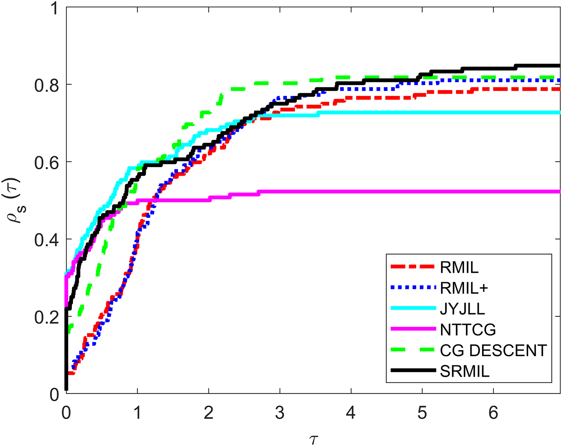
To evaluate and compare the performances of all the methods, we use the Dolan & Moré (2002) performance metrics tool. For every formula, the tool graphs the fraction of every problem solved based on the number of iterations (NOI) as shown in Fig. 1, number of functions evaluation (NOF) presented in Fig. 2 and CPU time given in Fig. 3. Note that the right side denotes the test functions successfully completed all the algorithms while the left-hand side of every graph represents the test problem percentage which defines the algorithm with better performance. The upper curve is the method with the best performance.
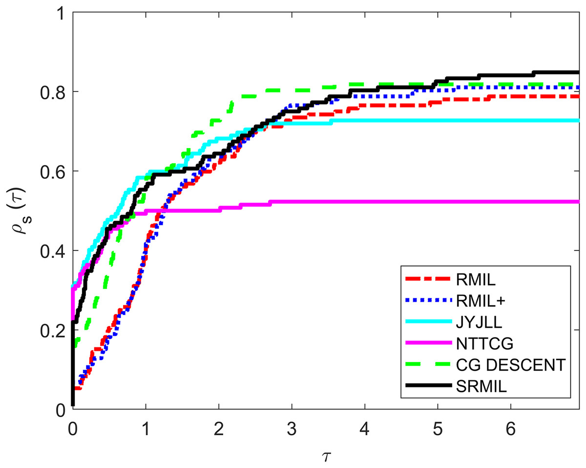
Figure 1: Performance metrics for NOI.
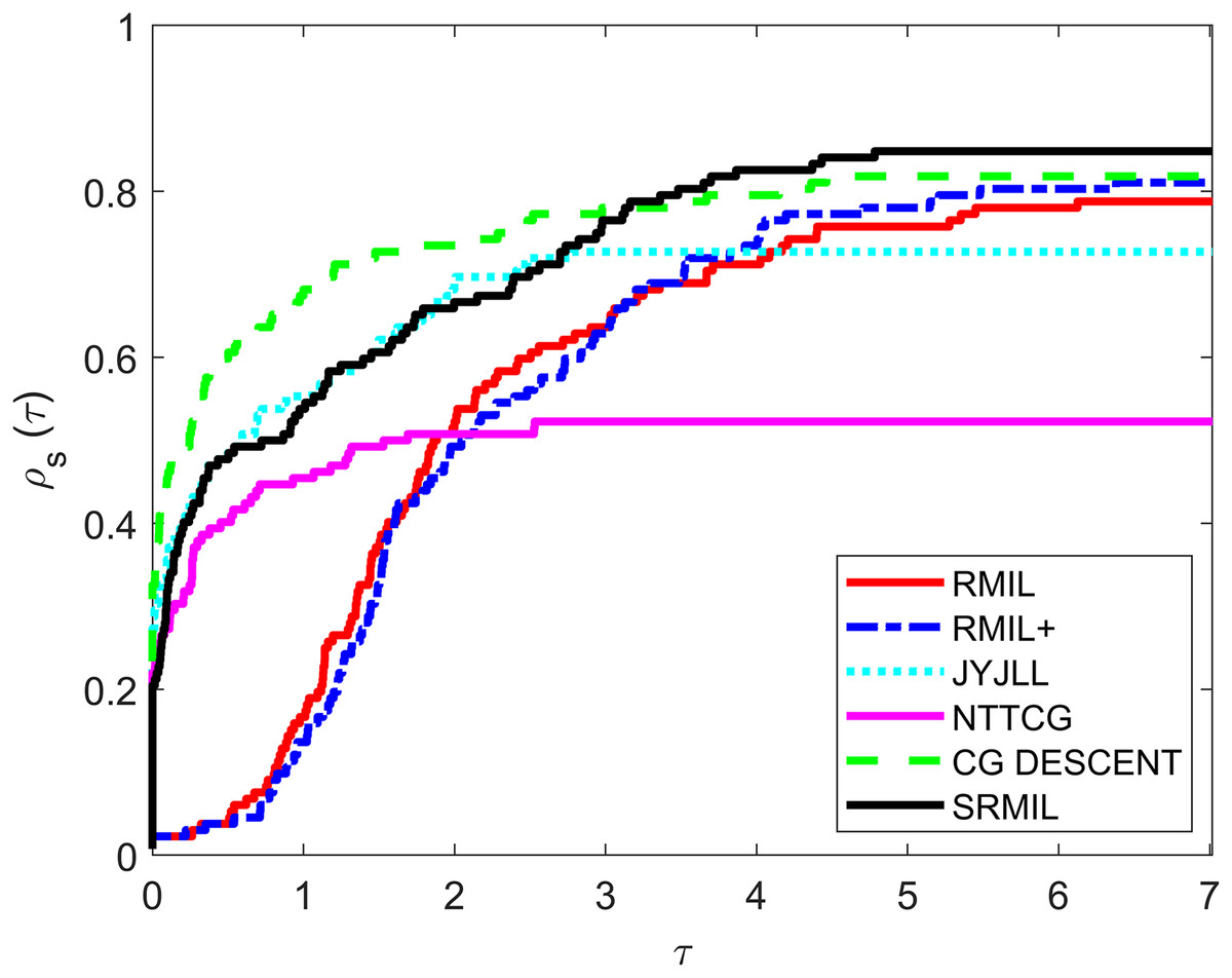
Figure 2: Performance metrics for NOF.
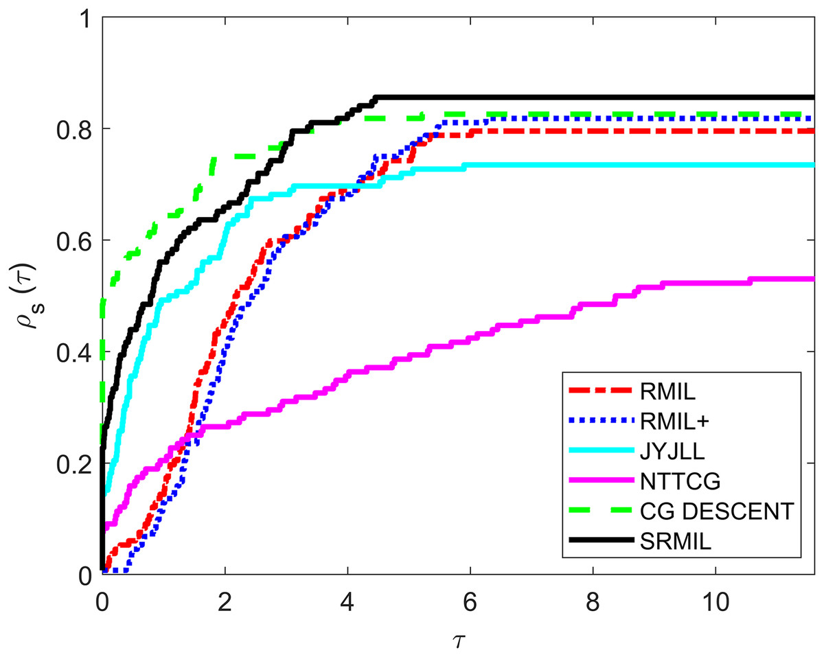
Figure 3: Performance metrics for CPU.
Observing all these graphs, we can see that the SRMIL formula is better than the RMIL, RMIL+, spectral JYJLL, NTTCG, and CG DESCENT methods because it converges faster and can complete more of the test functions.
Image restoration problem
This section investigates the performance of all the methods on image restoration models by recovering the original image from noisy or degraded versions. This is a specific form of unconstrained optimization problem, where the goal is to minimize the difference between the restored and original images. These problems are currently gaining a lot of attention in the research world due to their important applications in health and security (Malik et al., 2023; Yuan, Lu & Wang, 2020; Yu, Huang & Zhou, 2010; Salihu et al., 2023a). For this study, we consider restoring two images: CANAL and GARDEN that were corrupted by salt-and-pepper impulse noise. The quality of the restored image would be measured using peak signal-to-noise ratio (PSNR), relative error (RelErr), and CPU Time. The PSNR computes the ratio between the power of corrupting noises affecting fidelity of the representation and the maximum possible power of a signal. This metric is usually employed for measuring the qualities between the original and resultant images. A method with a higher PSNR value has better quality output images (Nadipally, 2019). The PSNR is computed as follows:
(27) where MSE denotes the mean square error used for assessing the average pixel differences for complete images and represents the image’s possible maximum pixel value. A high MSE value designates a greater difference between processed and original images. Yet, the edges have to be carefully considered. The MSE is computed as follows:
(28) where E denotes the edge image, and N defines the original image and image sizes, respectively.
Let define the real image with pixel, the image restoration problem is modeled into an optimization problem of the form:
and
where G denotes the index set of noise candidates define as:
(29)
Here, whose neighborhood is define as , and represent the maximum and minimum of a noisy pixel. The observed noisy image corrupted by salt-and-pepper impulse noise is given as and is the adaptive median filter of .
Also, in denotes an edge-preserving potential function define as
(30) where is a constant whose value is chosen as .
The performance results from the computational experiments are presented below.
Table 5 compares the performance of four methods (SRMIL, RMIL, RMIL+, and JYJLL) on image restoration models across different noise levels (30%, 50%, and 80%). Two images (“CANAL” and “GARDEN”) are considered, with CPU time (CPUT), relative error (RelErr), and peak signal-to-noise ratio (PSNR) used as evaluation metrics. SRMIL stands out as the fastest method, particularly at lower noise levels, where it provides competitive restoration results with minimal computational cost. While it shows slightly higher relative errors and lower PSNR at higher noise levels compared to RMIL+ and RMIL, it remains a highly efficient choice for scenarios where speed is critical. RMIL+ delivers a competitive performance at higher noise levels in terms of PSNR and relative error, but comes with a higher computational cost. RMIL offers a middle ground with moderate performance, while JYJLL is the least efficient in both quality and speed. Overall, SRMIL is the most efficient choice for speed and quality trade-offs, especially at lower noise levels, making it a strong option for time-sensitive applications.
| METHOD | SRMIL | RMIL | RMIL+ | JYJLL | |||||||||
|---|---|---|---|---|---|---|---|---|---|---|---|---|---|
| IMAGE | NOISE | CPUT | RelErr | PSNR | CPUT | RelErr | PSNR | CPUT | RelErr | PSNR | CPUT | RelErr | PSNR |
| CANAL | 30% | 48.4348 | 0.8080 | 31.4865 | 48.4444 | 0.7969 | 31.2218 | 48.5786 | 0.8270 | 31.2973 | 48.8289 | 0.7970 | 31.3173 |
| 50% | 131.7956 | 1.3664 | 28.0092 | 104.9128 | 1.3886 | 27.7759 | 107.4118 | 1.2796 | 27.8678 | 137.1973 | 1.2892 | 27.7886 | |
| 80% | 168.4606 | 2.1083 | 24.8027 | 200.8903 | 2.6569 | 23.1556 | 195.5230 | 2.6070 | 23.1988 | 196.3052 | 2.6798 | 23.1988 | |
| GARDEN | 30% | 63.5339 | 1.1222 | 28.5409 | 63.5676 | 1.1348 | 28.3746 | 62.6936 | 1.1634 | 28.3828 | 66.3669 | 1.1752 | 28.4827 |
| 50% | 128.4747 | 1.5731 | 25.5737 | 105.3938 | 1.7243 | 25.3806 | 227.0897 | 1.7072 | 25.2218 | 218.8192 | 1.7127 | 25.1822 | |
| 80% | 163.2581 | 2.2388 | 22.9950 | 195.6410 | 2.6818 | 21.7677 | 195.5568 | 2.7264 | 21.7584 | 181.9556 | 2.1472 | 21.8475 | |
The performance of SRMIL, RMIL, RMIL+, JYJLL was evaluated based on CPU Time, RelErr, and PSNR, as summarized in Table 5 with the graphical representation of the best performers presented in Figs. 4, 5, 6 respectively. It can be seen that all the methods are successful on all the perception-based quality metrics discussed earlier. However, the proposed method is acknowledged as the best performer because it produced the least CPU time and higher PSNR values for all the noise degrees. This is supported by the fact that a method with higher PSNR values produces better quality of the output images.
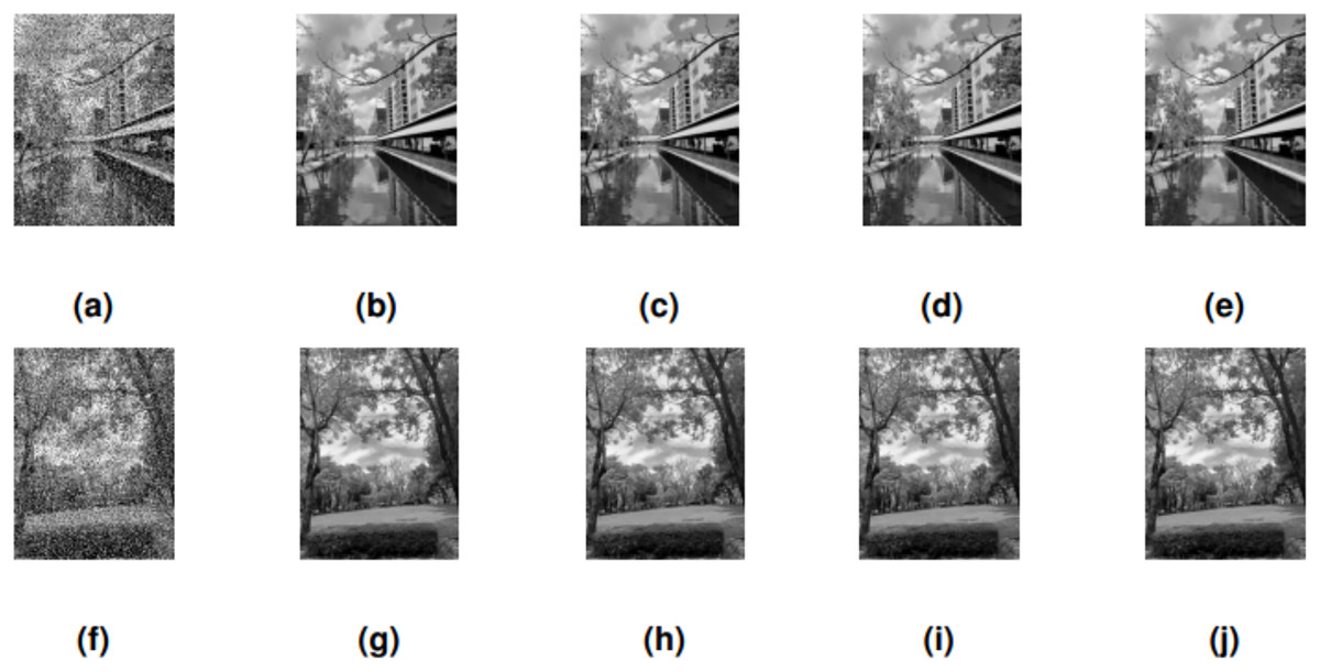
Figure 4: CANAL & GARDEN images corrupted by 30% salt-and-pepper noise: (A, F), the restored images using SRMIL: (B, G), RMIL: (C, H), and RMIL+: (D, I), and JYJLL: (E, J).
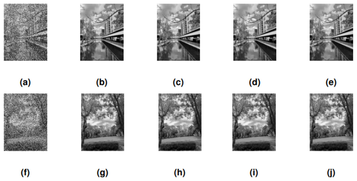
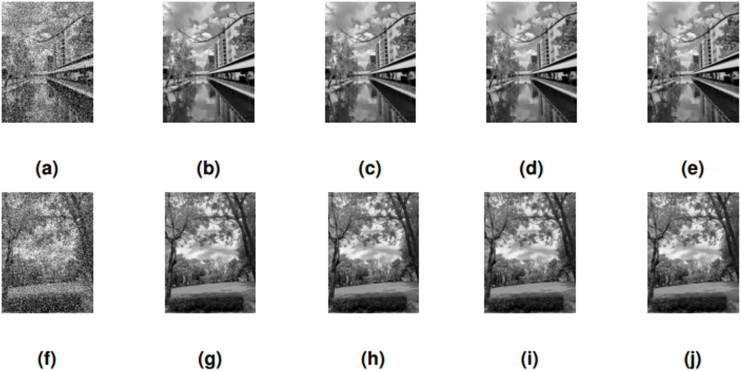
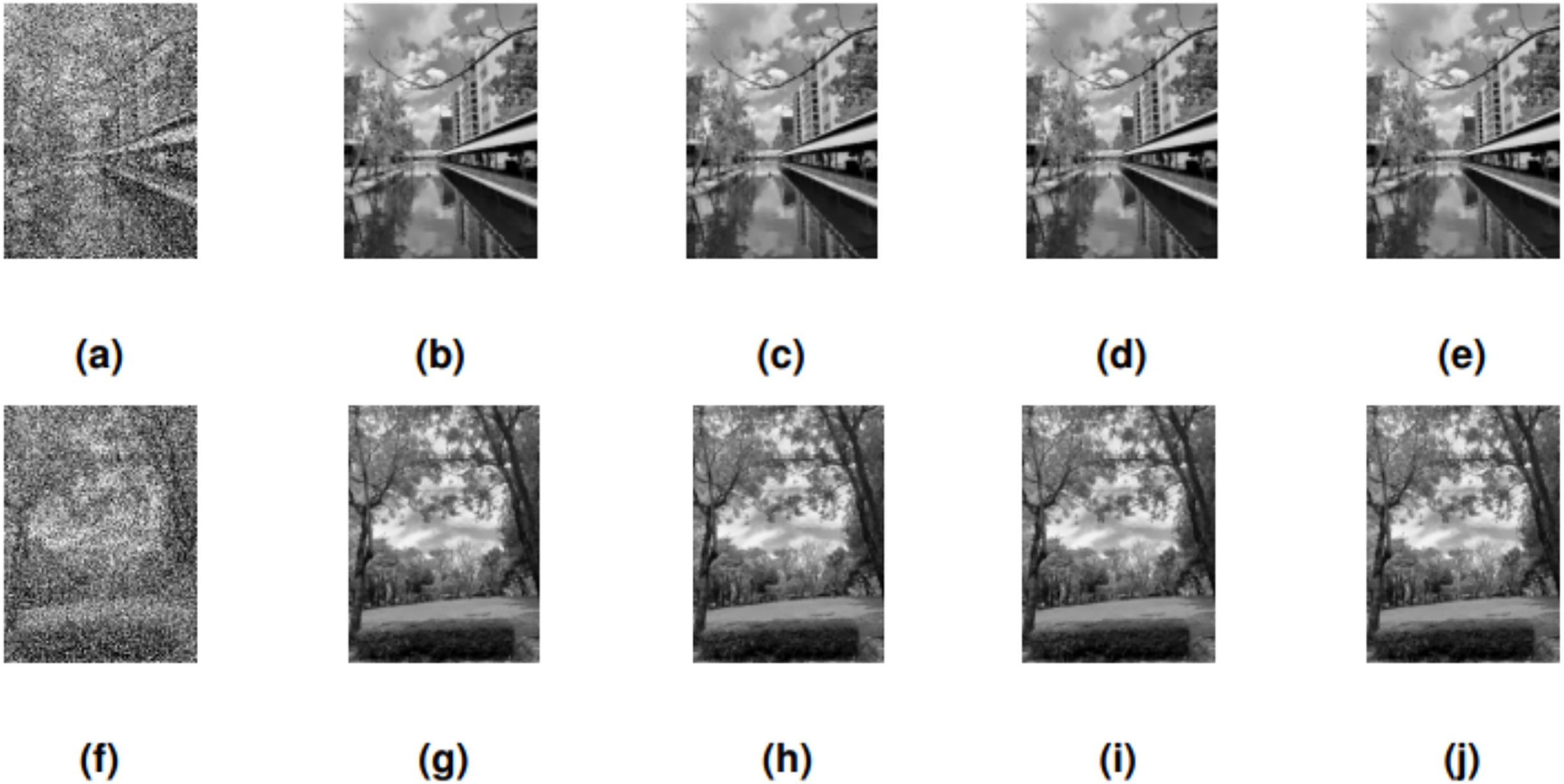
Figure 5: CANAL & GARDEN images corrupted by 50% salt-and-pepper noise: (A, F), the restored images using SRMIL: (B, G), RMIL: (C, H), and RMIL+: (D, I), and JYJLL: (E, J).
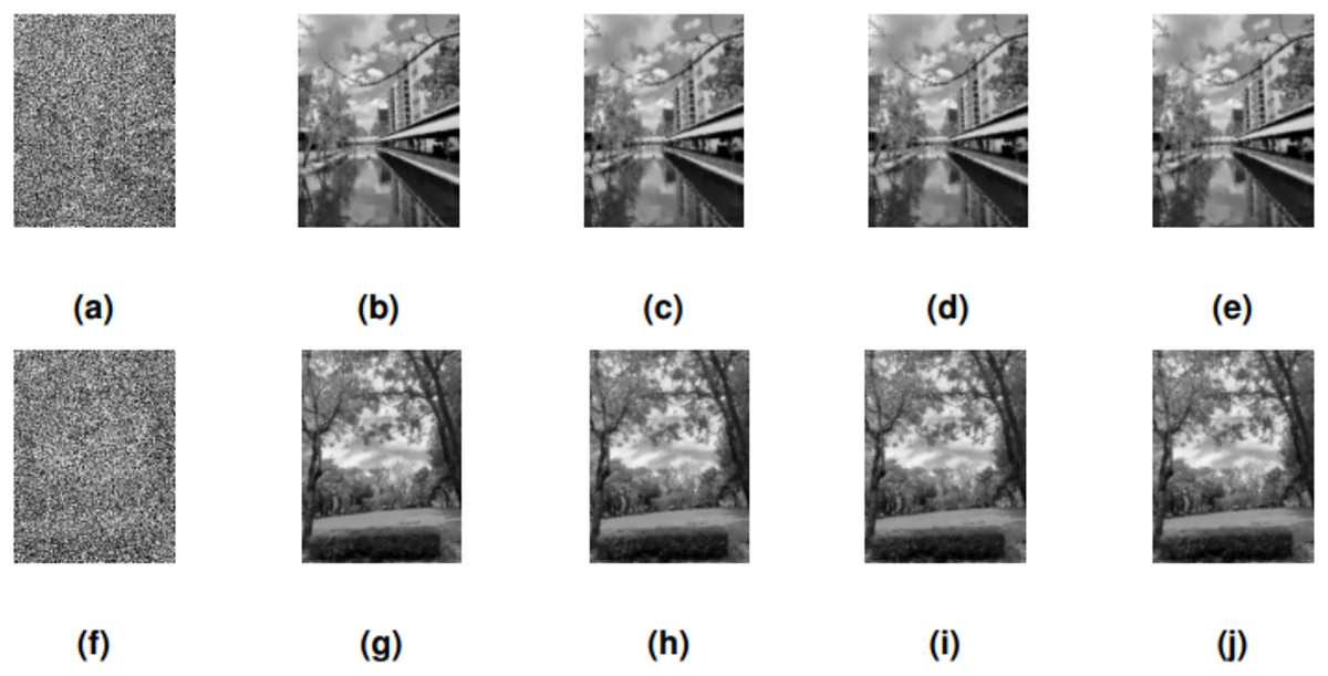
Figure 6: CANAL & GARDEN images corrupted by 80% salt-and-pepper noise: (A, F), the restored images using SRMIL: (B, G), RMIL: (C, H), and RMIL+: (D, I), and JYJLL: (E, J).
Therefore, this demonstrates the importance of the proposed algorithm in solving some applications as well as highlighting some challenges of developing new iterative algorithm for real-life problems.
Application in robotic arm motion control
Robotic motion control are processes and systems employed to control the movement of robots. This field encompasses different technologies and techniques to ensure efficient and accurate movement of robotic systems. Some real-world applications of these robots include industrial automation where the robots perform tasks such as packaging, painting, welding, and assembly. Also, service robots assist in hospitality or household chores while medical robots include rehabilitation devices and surgical robots. The major problem of robotic motion control often arises as a result of various factors including dynamic uncertainties, actuator limitations, sensor noise, and environmental disturbances. For instance, the robot may fail to follow the desired path accurately due to non-linearities, delays, disturbances, and inaccurate modeling. This problem can be overcome by adaptive control to adjust the parameters in real time or by using advanced control techniques such as the currently used gradient-based methods.
In this study, the application of the proposed gradient-based SRMIL algorithm will be demonstrated on a simulated robotic model. Our approach leverages the conjugate gradient (CG) method within an inverse kinematics framework to optimize joint angles to achieve desired end-effector positions. Specifically, we solve non-linear systems formulated from the kinematic equations of the robotic arm, where the proposed CG method is used to iteratively refine joint parameters to minimize positioning error.
The robotic model, originally defined with two degrees of freedom (2DOF) as detailed in Sulaiman et al. (2022) and Awwal et al. (2021), has currently been extended to include three degrees of freedom (3DOF) (Yahaya et al., 2022; Yunus et al., 2023). Noted that the scope of this study for robotic motion control is limited to a simulated 3DOF robotic system. This system is designed to evaluate the algorithm’s capability to handle trajectory optimization and precision control challenges. The problem description begins with an illustration of the planar three-joint kinematic model equation and the formulation of the discrete kinematic model equation for three degrees of freedom as presented in Yahaya et al. (2022), Zhang et al. (2019), Yunus et al. (2023).
(31) where and denote the end vector effector position and the joint angle vector respectively. with denoting the joint angle vector, defining the end vector effector position, and the function representing the kinematic mapping whose equation is formulated as follows:
(32) with , , and represent the first, second and their rod lengths respectively. The function is responsible for mapping the active joint displacements to any part of the robot or position and orientation of a robot’s end-effector. In the case of robotic motion control, represents the end-effector position vector. To achieve the problem formulation at a specific moment , we define the preferred path vector as . Based on the preferred path vector, we can now formulate the following least-squares problem which is addressed at every interval :
(33) where denotes the end effector controlled track and as described in Yahaya et al. (2022), the Lissajous curves route required at time are generated using:
(34)
(35)
(36)
Observe that the structure of Eq. (33) is similar to that of 1 defined earlier which enables utilizing the proposed SRMIL algorithm to solve this problem. For the experiment simulation, the parameters used in the implementation are , and s. Each link is connected by a rotational joint, enabling motion within a two-dimensional workspace. The starting point with the duration of task divided into equal segments, providing a structured timeline for the optimization process and allowing precise evaluation of the method’s performance over time. The joint angles , , and determine the configuration of the arm, and the position of the end effector is denoted by . This planar configuration ensures that the arm can achieve various positions within its workspace, constrained by the total link lengths and joint angles. The following algorithm describe the procedure used in solving the problem.
The experimental results of the SRMIL for motion control are demonstrated in Figs. 7–10.
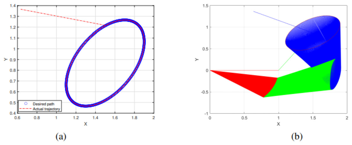
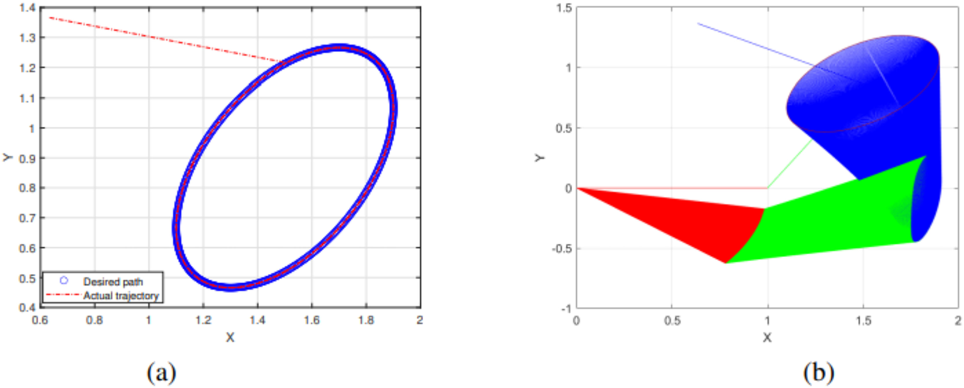
Figure 7: End effector trajectory and desired path (A) and Synthesized robot trajectories of Lissajous curve (Eq. (34)).
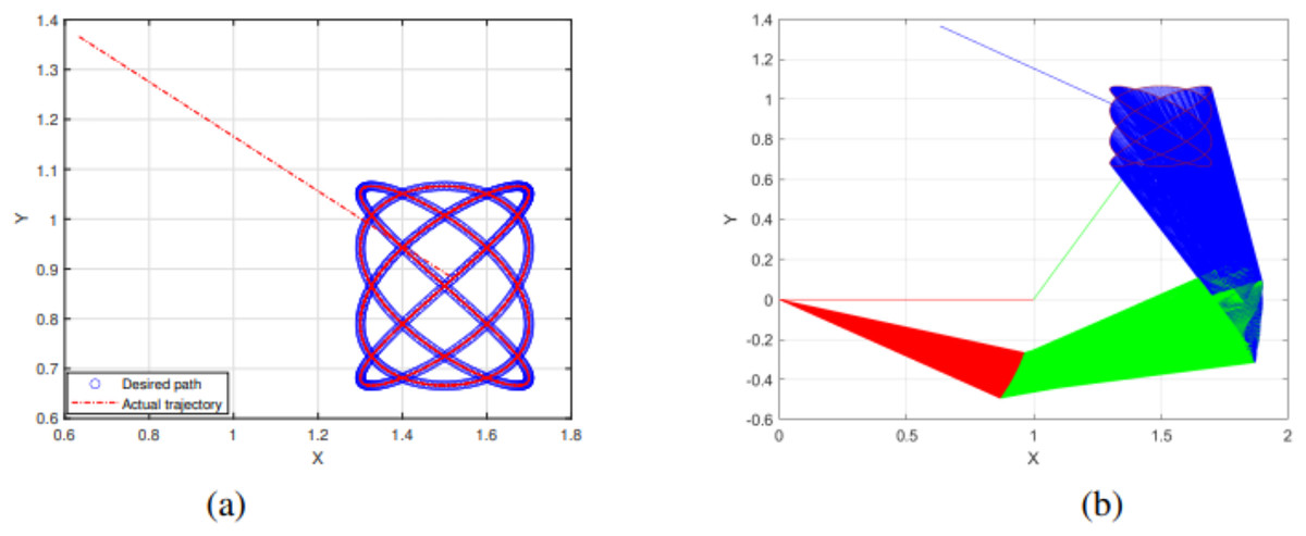
Figure 8: End effector trajectory and desired path (A) and Synthesized robot trajectories of Lissajous curve (Eq. (35)).
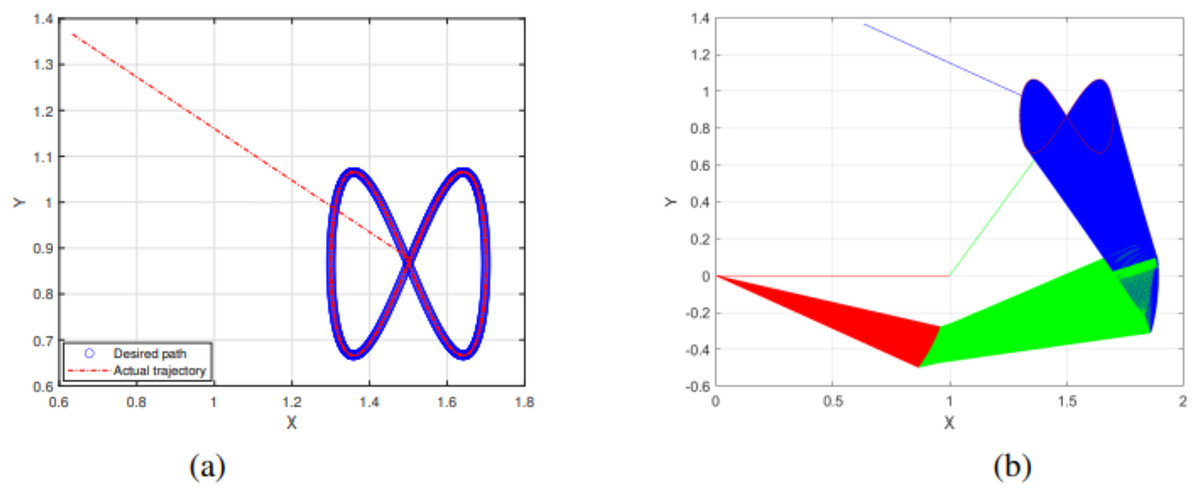
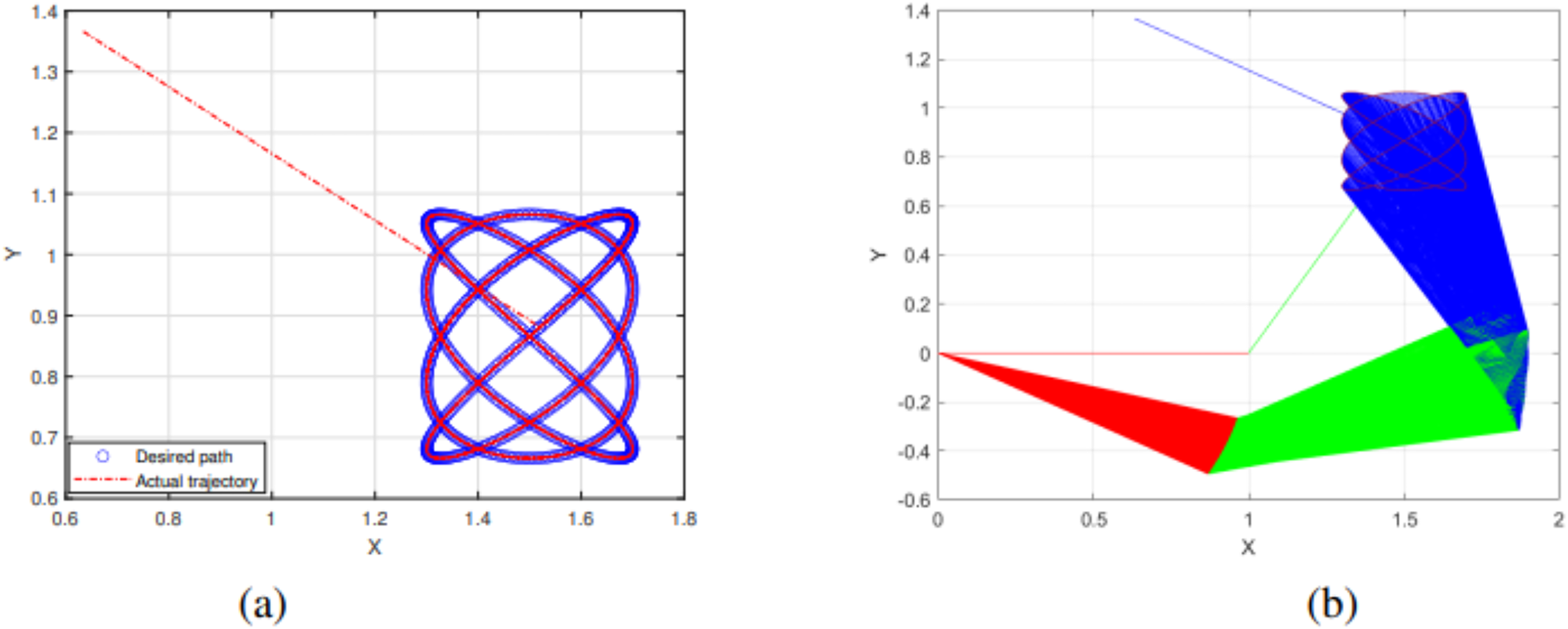
Figure 9: End effector trajectory and desired path (A) and Synthesized robot trajectories of Lissajous curve (Eq. (35)).
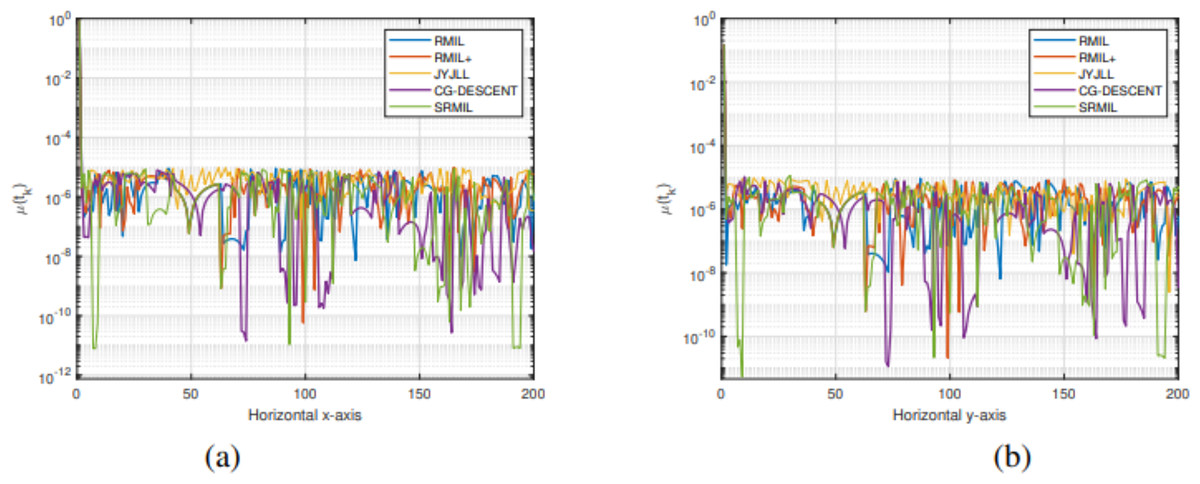
Figure 10: Tracking the residual error of Lissajous curve along axes (A), along axes (B).
The detailed explanation of the results is as follows. Figures 7A, 8A, and 9A demonstrate the robot’s end effector model precisely following the desired path of Lissajous curve Eqs. (34)–(36), respectively. While Figs. 7B, 8B, and 9B illustrate the synthesis of the robot’s trajectories of the Lissajous curve Eqs. (34), (35) and (36), respectively. Figures 10A and 10B represent the error rates of residuals, indicating that SRMIL recorded the least errors despite the close competition the method faced from the classical CG-DESCENT algorithm. The higher residual errors observed in existing methods might be due to limitations in their ability to handle nonlinearities in robotic motion control tasks. On the other hand, the low residual error rates recorded by the proposed SRMIL algorithm can be attributed to its ability to efficiently handle the complexities and dynamics requirements of the considered problems, and thus, demonstrate its efficiency and robustness in practical application.
The study further compared the performance of the algorithms including SRMIL, JYJLL, RMIL+, and RMIL on Lissajous curve problems (see; Table 6), using computational time (CPUT) and iteration count (Iter) as evaluation metrics. For clarity, we bolded the best results to easily differentiate the performance of the algorithms.
| METHOD | SRMIL | JYJLL | RMIL+ | RMIL | |||||
|---|---|---|---|---|---|---|---|---|---|
| LISSAJOUS CURVES | EQUATION | CPUT | Iter | CPUT | Iter | CPUT | Iter | CPUT | Iter |
| (34) | 0.3839 | 64 | 0.3972 | 81 | 0.3672 | 62 | 0.3893 | 65 | |
| (35) | 0.3592 | 27 | 0.4000 | 30 | 0.3688 | 29 | 0.3597 | 27 | |
| (36) | 0.3175 | 38 | 0.4246 | 43 | 0.3173 | 38 | 0.3149 | 37 | |
Note:
Best results are in bold.
As observed in Table 6, the proposed SRMIL demonstrates strong performance, achieving competitive or superior results in both metrics across all cases. RMIL+ closely rivals SRMIL, especially for , where it achieves the fastest computational time and fewest iterations. RMIL shows consistent, reliable performance, slightly trailing SRMIL and RMIL+ in most cases. On the other hand, JYJLL is the least efficient, with higher iteration counts and computational times across all problems. Overall, SRMIL and RMIL+ emerge as the most effective algorithms, excelling in both iteration count and efficiency, while RMIL remains a strong alternative. JYJLL’s relatively poor performance indicates it may require further refinement for problems of this type. These results further demonstrate the potential of SRMIL and RMIL+ for solving optimization problems involving Lissajous curves, with SRMIL offering the best balance of computational efficiency and convergence behavior.
Conclusions
In this article, we have presented a descent modification of the RMIL+ CG algorithm such that the coefficient does not become superfluous. The proposed method was further extended to construct a new search direction that guarantees a sufficient decrease in the objective function. The global convergence was discussed using the Lipschitz continuity assumption. Numerical results on a range of test problems were reported to evaluate the algorithm’s performance. Specifically, the new method demonstrated consistent effectiveness by outperforming other algorithms, including CG-DESCENT, in terms of iteration counts and function evaluations. Robustness was assessed by testing the algorithm on problems with varying dimensions and initial points. Additionally, the practical applicability of the proposed algorithm was validated through detailed comparisons in image restoration and 3DOF robotic motion control simulation involving a generic 3DOF system designed to capture typical challenges in trajectory optimization. Future work will involve additional tests of the proposed algorithm, including sensitivity analyses and real-world scenarios, such as experiments with actual robotic systems, to further substantiate its robustness.