
Symbolic model checking quantum circuits in Maude
- Published
- Accepted
- Received
- Academic Editor
- Marieke Huisman
- Subject Areas
- Emerging Technologies, Theory and Formal Methods, Programming Languages, Software Engineering, Quantum Computing
- Keywords
- Quantum circuits, Dirac notation, Symbolic model checking, Maude
- Copyright
- © 2024 Minh Do and Ogata
- Licence
- This is an open access article distributed under the terms of the Creative Commons Attribution License, which permits unrestricted use, distribution, reproduction and adaptation in any medium and for any purpose provided that it is properly attributed. For attribution, the original author(s), title, publication source (PeerJ Computer Science) and either DOI or URL of the article must be cited.
- Cite this article
- 2024. Symbolic model checking quantum circuits in Maude. PeerJ Computer Science 10:e2098 https://doi.org/10.7717/peerj-cs.2098
Abstract
This article presents a symbolic approach to model checking quantum circuits using a set of laws from quantum mechanics and basic matrix operations with Dirac notation. We use Maude, a high-level specification/programming language based on rewriting logic, to implement our symbolic approach. As case studies, we use the approach to formally specify several quantum communication protocols in the early work of quantum communication and formally verify their correctness: Superdense Coding, Quantum Teleportation, Quantum Secret Sharing, Entanglement Swapping, Quantum Gate Teleportation, Two Mirror-image Teleportation, and Quantum Network Coding. We demonstrate that our approach/implementation can be a first step toward a general framework to formally specify and verify quantum circuits in Maude. The proposed way to formally specify a quantum circuit makes it possible to describe the quantum circuit in Maude such that the formal specification can be regarded as a series of quantum gate/measurement applications. Once a quantum circuit has been formally specified in the proposed way together with an initial state and a desired property expressed in linear temporal logic (LTL), the proposed model checking technique utilizes a built-in Maude LTL model checker to automatically conduct formal verification that the quantum circuit enjoys the property starting from the initial state.
Introduction
Quantum computing is a rapidly emerging technology that uses the laws of quantum mechanics to solve complex problems that are very hard for classical computers, such as discrete logarithms and factoring. Several quantum algorithms have been proposed showing a significant improvement over classical algorithms, such as the fast algorithms for discrete logarithms and factoring proposed by Shor (1994). It is well known that cryptosystems relying on the hardness of discrete logarithms and factoring will be broken by large-scale quantum computers running Shor’s fast algorithm in the future. Then, quantum communication involving quantum cryptography has attracted much attention from both industry and academia because it provides an efficient and highly secure communication channel relying on quantum mechanics phenomena, such as superposition, entanglement, and probabilistic measurement.
Quantum circuits are a model of quantum computation, comprising a sequence of quantum gates, measurements, initializations of qubits, and possibly other actions. Quantum gates operate on quantum bits (qubits), the quantum counterpart of classical bits, and manipulate the state of a quantum system to perform quantum computations. The outputs of quantum circuits are quantum states, which can be measured to obtain classical outcomes with probabilities from which other actions can take place. Quantum circuits play a crucial role in the development of quantum algorithms because they are used to design and implement quantum algorithms before actually running on quantum computers. Because quantum computing is counter-intuitive and radically different from classical computing, the likelihood of errors in quantum algorithms and circuits is much higher than in classical algorithms. Therefore, it is critical to verify that quantum circuits (or algorithms) enjoy desired properties.
Model checking is a formal verification technique widely used in both academia and industry to systematically verify that systems satisfy desired properties. Quantum programs and quantum circuits are related concepts, but they differ in their level of abstraction and the way they represent quantum computations. Quantum circuits are low-level representations of quantum computation that can be used to implement quantum programs, while quantum programs are higher-level representations of quantum computations that can be expressed in a quantum programming language consisting of a series of instructions, especially the loop instruction. Although there are some model checkers dedicated to quantum programs, such as Gay, Nagarajan & Papanikolaou (2008), Feng, Yu & Ying (2013) and Feng et al. (2015) (see Ying & Feng (2018), Ying & Feng (2021), Turrini (2022) for more details), there is still a gap between model checking quantum programs and quantum circuits due to different representations and no iteration in quantum circuits, which should be filled in. Moreover, because the verification of classical circuits using model checking has been proven to be a tremendously successful technique, model checking that quantum circuits satisfy desired properties would be a promising approach. There is a symbolic approach proposed by Shi et al. (2021) to (semi-)automatically reasoning about quantum circuits in Coq (https://coq.inria.fr/), an interactive theorem prover, but it often requires human users to provide necessary lemmas to complete its proofs.
This article presents a symbolic approach to model checking quantum circuits using a set of laws from quantum mechanics and basic matrix operations with Dirac notation proposed by Dirac (1939). Concretely, quantum states, quantum gates, and measurements are described in Dirac notation instead of using explicitly complex vectors and matrices as proposed by Paykin, Rand & Zdancewic (2017), making our representations more compact. Using the set of laws, we can systematically reason about the evolution of quantum states. We use Maude introduced by Clavel et al. (2007), a high-level specification/programming language based on rewriting logic presented by Meseguer (2012), to specify quantum states, some basic quantum gates (e.g., Hadamard gate, controlled-NOT gate, and Pauli gates), and measurements on a standard basis with Dirac notation. Maude is equipped with a linear temporal logic (LTL) model checker and its reflective programming (or meta-programming) facilities have been used to develop several software tools, such as Maude-NPA introduced by Escobar, Meadows & Meseguer (2007), its parallel version developed by Do et al. (2022), and a toolset of some parallel versions of the LTL model checker presented by Do et al. (2021), Do, Phyo & Ogata (2022), Do et al. (2023) and Phyo et al. (2023). Therefore, Maude makes it possible/convenient to implement our idea and carry out case studies. This is why we adopt Maude for the research described in the article.
As case studies, we focus on using our approach to formally specify several quantum communication protocols in the early work of quantum communication and formally verify their correctness: Superdense Coding introduced by Bennett & Wiesner (1992), Quantum Teleportation presented by Bennett et al. (1993), Quantum Secret Sharing developed by Hillery, Bužek & Berthiaume (1999), Entanglement Swapping proposed by Zukowski et al. (1993), Quantum Gate Teleportation suggested by Gottesman & Chuang (1999), Two Mirror-image Teleportation devised by Williams (2008), and Quantum Network Coding originated by Satoh, Gall & Imai (2012). In this article, we use eventual properties, a class of liveness properties, to express the desired properties for these quantum communication protocols. In addition to the desired properties, any properties that can be expressed in the scope of LTL can essentially be verified using the Maude LTL model checker with our approach. In this article, we do not directly tackle quantum circuits for complicated quantum algorithms, such as Shor (1994) and Grover (1996) because necessary quantum gates have not been developed yet and our symbolic reasoning for complex numbers is not sufficient to describe and reason about their behaviors adequately. Therefore, extending our approach to handle these algorithms would require further research, which would be one piece of our future work. Our specification is specifically tailored to quantum circuits, abstracting away from the details of concurrency and communication. To handle quantum cryptography, such as BB84 introduced by Bennett & Brassard (2014) and B91 introduced by Ekert (1991), we need to be able to express concurrency and communication among participants in quantum protocols in our specification. Therefore, extending our approach to handle such quantum protocols would require further research, which would be one piece of our future work.
We demonstrate that our approach/implementation can be a first step toward a general framework to formally specify and verify quantum circuits. The proposed way to formally specify a quantum circuit makes it possible to describe the quantum circuit in Maude such that the formal specification can be regarded as a series of quantum gate/measurement applications. Once a quantum circuit has been formally specified in the proposed way together with an initial state and a desired property expressed in LTL, the proposed model checking technique utilizes a built-in Maude LTL model checker to automatically conduct formal verification that the quantum circuit enjoys the property starting from the initial state. Moreover, our specification considers the probabilities from measurements in quantum computation based on which the probability of a computation occurring is accumulated across states and so we are able to analyze both the quantitative and qualitative properties1 of several quantum communication protocols with the built-in LTL model checker in Maude. Our implementation is publicly available at https://doi.org/10.5281/zenodo.10783951.
The present article is an extended and improved version of our conference article presented by Do & Ogata (2023) with some improvements as follows:
-
We fully support Pauli gates in our specification and some additional gates, including S, T, CY, CZ, SW AP, CCY, CCZ, and CSW AP gates. Moreover, the symbolic reasoning is refined and improved in order to conduct more case studies.
-
We verify some more quantum communication protocols: Superdense Coding, Quantum Secret Sharing, Entanglement Swapping, Quantum Gate Teleportation, Two Mirror-image Teleportation, and Quantum Network Coding in order to demonstrate the usefulness of our approach for formally specifying and verifying quantum circuits in Maude.
-
We identify that the original version of Quantum Gate Teleportation does not satisfy its desired property using our approach and support tool. We then propose a revised version of the protocol and verify that the revised one satisfies its desired property using our approach and support tool.
-
Lastly, we describe how we specify complex numbers in Maude to symbolically reason on complex numbers with rational numbers for our case studies.
The rest of the article is organized as follows: ‘Preliminaries’ explains basic quantum mechanics and Kripke structures; ‘Rewriting Logic and Quantum Circuits’ explains how we can associate a rewrite theory with a quantum circuit via a Kripke structure; ‘Symbolic Reasoning’ describes how to construct terms and use a set of laws from quantum mechanics and matrix operations for symbolic reasoning using our approach; ‘Formal Specification’ details how to specify qubits, gates, measurements, and then quantum circuits in order to symbolically model check quantum circuits in a generic way; ‘Symbolic Model Checking’ demonstrates how to use our symbolic approach to model checking several quantum communication protocols in depth; ‘Remark on Quantum Gate Teleportation’ provides a remark on Quantum Gate Teleportation; ‘Experimental Results’ presents our experimental results; ‘Discussion’ discusses our limitations, some challenges in using the Maude LTL model checker, a classical model checker, to verify quantum circuits, and how we address them in this article; ‘Related Work’ reviews some existing work; and ‘Conclusion’ concludes the article with some pieces of future work.
Preliminaries
This section briefly describes some basic notations from quantum mechanics based on linear algebra (refer to Nielsen & Chuang (2010) for more details) and Kripke structures.
Basic quantum mechanics
This section describes basic quantum mechanics based on the linear algebra approach. In classical computing, the fundamental unit of information is a bit whose value is either 0 or 1. In quantum computing, the counterpart is a quantum bit or qubit, which has two basis states, conventionally written in Dirac notation proposed by Dirac (1939) as |0〈.〉 and |1〈.〉, which denote two column vectors and , respectively. In quantum theory, a general state of a quantum system is a superposition or linear combination of basis states. A single qubit has state |ψ〈.〉 = α|0〈.〉 + β|1〈.〉, where α and β are complex numbers such that |α|2 + |β|2 = 1. States can be represented by column complex vectors as follows:
,
where {|0〈.〉, |1〈.〉} forms an orthonormal basis of the two-dimensional complex vector space. Formally, a quantum state is a unit vector in a Hilbert space , which is equipped with an inner product satisfying some axioms.
The basis {|0〈.〉, |1〈.〉} is called the standard basis. Besides, we have some other bases of interest, such as the diagonal (or dual, or Hadamard) basis consisting of the following vectors:
and .
The evolution of a closed quantum system can be performed by a unitary transformation. If the state of a qubit is represented by a column vector, then a unitary transformation can be represented by a complex-value matrix U such that UU† = U†U = I or U† = U−1, where U† is the conjugate transpose of U. U acts on the Hilbert space transforming a state |ψ〈.〉 to a state |ψ′〈.〉 by a matrix multiplication such that |ψ′〈.〉 = U|ψ〈.〉. There are some common quantum gates: the identity gate I, the Pauli gates X, Y, and Z, the Hadamard gate H, and the controlled-NOT gate CX. Note that the CX gate performs on two qubits, while the remaining gates perform on a single qubit.
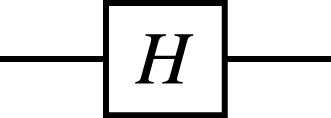
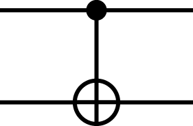
For example, the Hadamard gate on a single qubit performs the mapping and . The controlled-NOT gate on pairs of qubits performs the mapping |00〈.〉↦|00〈.〉, |01〈.〉↦|01〈.〉, |10〈.〉↦|11〈.〉, |11〈.〉↦|10〈.〉, which can be understood as inverting the second qubit (referred to as the target) if and only if the first qubit (referred to as the control) is 1. The common quantum gates are shown in Table 1 by names, circuit forms, and matrix representations, where i is the imaginary unit.
| Operator | Gate | Matrix |
|---|---|---|
| Identity (I2) |
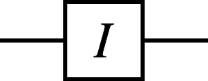
|
|
| Pauli-X (X) |
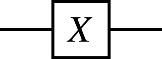
|
|
| Pauli-Y (Y) |
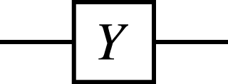
|
|
| Pauli-Z (Z) |
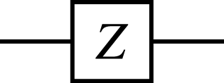
|
|
| Hadamard (H) |
|
|
| Controlled-NOT (CX) (the first and second wires denote the control and target qubits, respectively) |
|
A quantum measurement is described as a collection {Mm} of measurement operators, where the indices m refer to the measurement outcomes. It is required that the measurement operators satisfy . If the state of a quantum system is |ψ〈.〉 before the measurement, then the probability for the result m is as follows:
,
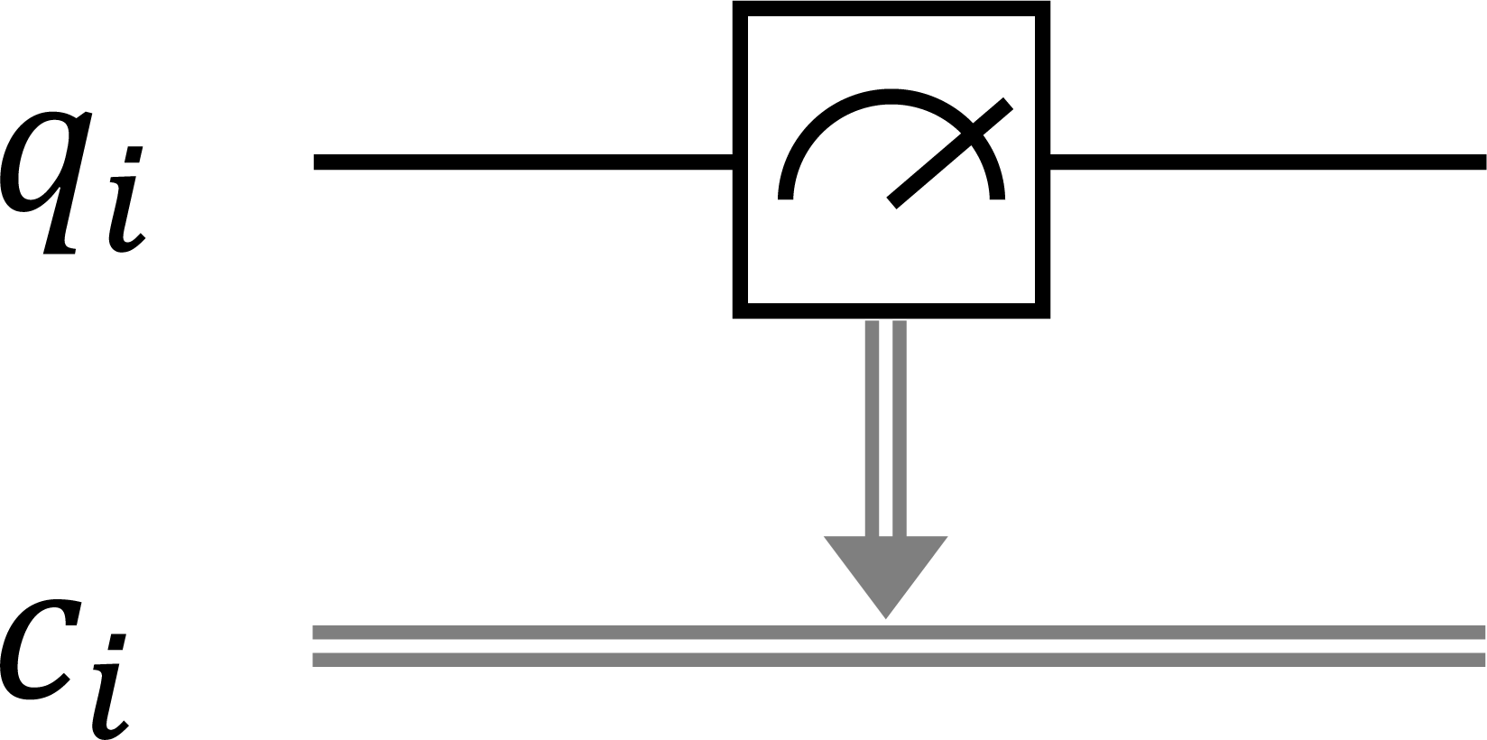
where 〈〉.ψ| is the dual of |ψ〈.〉 such that 〈〉.ψ|† = |ψ〈.〉 and |ψ〈.〉† = 〈〉.ψ|. The state of the quantum system after the measurement is provided that p(m) > 0. For example, if a qubit is in state α|0〈.〉 + β|1〈.〉 and measuring with {M0, M1} operators, we have the result 0 with probability |α|2 at the post-measurement state |0〈.〉 and the result 1 with probability |β|2 at the post-measurement state |1〈.〉, where M0 = |0〈.〉 × 〈〉.0| and M1 = |1〈.〉 × 〈〉.1|. The quantum measurement with {M0, M1} operators is called the binary projective measurement. In this study, we only use the binary projective measurement and its circuit form is depicted in Fig. 1 as follows:

Figure 1: The circuit form of the binary projective measurement, where the measurement outcome of the qubit qi is stored in the classical bit ci.
For multiple qubits, we use the tensor product of Hilbert spaces. Let and be two Hilbert spaces. Their tensor product is defined as a vector space consisting of linear combinations of the vectors |ψ1ψ2〈.〉 = |ψ1〈.〉|ψ2〈.〉 = |ψ1〈.〉⊗|ψ2〈.〉, where and . Systems of two or more qubits may be in entangled states, meaning that states of qubits are correlated and inseparable. For example, we consider a measurement of the first qubit of the entangled state . The result is either 0 with probability leaving its state |00〈.〉 or 1 with probability leaving its state |11〈.〉. In either case, a subsequent measurement of the second qubit gives a non-probabilistic result, which is immediate to the result of the first measurement before. Entanglement shows that an entangled state of two qubits cannot be expressed as a tensor product of single-qubit states. We can use H and CX gates to create entangled states as follows: .
Kripke structures
A Kripke structure K is a tuple 〈S, I, T, A, L〉 as represented by Clarke et al. (2018), where S is a set of states, I⊆S is the set of initial states, T⊆S × S is a left-total binary relation over S, A is a set of atomic propositions, and L is a labeling function whose type is S → 2A. Each element (s, s′) ∈ T is called a state transition from s to s′ and T may be called the state transitions (with respect to K). For a state s ∈ S, L(s) is the set of atomic propositions that hold in s. A path π is an infinite sequence s0, …, si, si+1, … such that si ∈ S and (si, si+1) ∈ T for each i. We use the following notations for paths: πi≜si, si+1, …, πi≜s0, …, si, si, si, …, π(i)≜si, where ≜ is used as “be defined as.” πi is obtained by deleting the first i states s0, s1, …, si−1 from π. πi is obtained by taking the first i + 1 states s0, s1, …, si−1, si and adding si unboundedly many times at the end. π(i) is the ith state si. Let be the set of all paths. π is called a computation if π(0) ∈ I. Let be the set of all computations.
The syntax of a formula φ in LTL for K is as follows:
where p ∈ A, and and are called the next temporal connective and the until temporal connective, respectively. We introduce the eventual temporal abbreviation ♢ which is defined as follows:
This eventual temporal abbreviation is also used in Clarke et al. (2018).
Let be the set of all formulas in LTL for K. Given an arbitrary path of K and an arbitrary LTL formula of K, K, π⊧φ is inductively defined as follows:
-
K, π⊧⊤
-
K, π⊧p iff p ∈ L(π(0))
-
K, π⊧¬φ1 iff K, π⁄⊧φ1
-
K, π⊧φ1∧φ2 iff K, π⊧φ1 and K, π⊧φ2
-
iff K, π1⊧φ1
-
iff there exists a natural number i such that K, πi⊧φ2 and for all natural numbers j < i, K, πj⊧φ1
where φ1 and φ2 are LTL formulas. Then, K⊧φ iff K, π⊧φ for each computation of K.
In this article, we refer to ♢φ as eventual properties, which informally state that something will eventually happen. Termination or halting is one important system requirement that many systems should satisfy and can be expressed in LTL as an eventual property. Moreover, we aim to verify whether quantum circuits satisfy certain desired properties where something good eventually happens. For example, a qubit at the final state for each possible execution path is the same as another qubit at the initial state with a non-zero probability. Therefore, it is worthwhile to use eventual properties to express desired properties for our case studies under verification. For more details, the reader is referred to ‘Symbolic Model Checking’ to see how we express the desired properties for our case studies as eventual properties.
Rewriting Logic and Quantum Circuits
This section describes how we can associate a rewrite theory with a quantum circuit via a Kripke structure at a conceptual level, enabling the use of LTL model checking to verify that the quantum circuit enjoys a desired property.
A rewrite theory is a triple (Σ, E, R), where
-
Σ is an order-sorted signature consisting of a set of sorts, subsorts, and function symbols,
-
(Σ, E) forms an order-sorted equational theory with E being a collection of (possibly conditional) equations t = t′,
-
R is a collection of (possibly conditional) rewrite rules l → r.
Terms are built from variables, constants, and function symbols from Σ, and each term has a sort. The equations in E are used to reduce a term into a normal form, while the rewrite rules in R modulo E are used to make local transitions in systems, making it possible to rewrite one term to another term. We can associate a Kripke structure K = 〈S, I, T, A, L〉 to a rewrite theory as presented in Clavel et al. (2007, Chapter 13). In short, each term t in can be regarded as a state s ∈ S in K; and each rewriting step from t to t′ can be regarded as a state transition (s, s′) ∈ T in K, where t and t′ are terms of the same sort with their corresponding states s, s′ ∈ S. A and L are not necessary parts of and can be specified later in terms of constants and equations, respectively, to determine whether atomic propositions are true at a given state.
A quantum circuit can be described as a series of applications of quantum gates, measurements, and conditional gates, which are applied based on the outcomes of measurements. The input of a quantum circuit is a quantum state, and so is the output. The input and the output of a quantum circuit can be regarded as the initial state and the final state belonging to S in K, where the initial state also belongs to I in K. Therefore, a quantum state can be specified as a term in the rewrite theory . The application of quantum gates manipulates a quantum state to perform quantum computation, which is specified in terms of equations in so that we can reason about quantum computation. The application of a quantum gate can be regarded as a deterministic state transition in K since it transforms a quantum state into another quantum state. As a result, the application of a quantum gate can be specified by a rewrite rule in . Besides quantum gates, we can conduct a measurement on a quantum state to obtain classical outcomes based on which other quantum actions (e.g., quantum gates) can take place. As mentioned before, we are only interested in the binary projective measurement in this article. Therefore, the application of a measurement can be regarded as a non-deterministic state transition in K since the measurement may make a quantum state collapse into one of two different possibilities of quantum states with probabilities. As a result, the application of a measurement can be specified by two rewrite rules in . Note that there are only two rewrite rules for quantum measurements, while there are as many rewrite rules as the number of quantum gates supported by the rewrite theory . If the equations in are sufficient to reason about any quantum computation and the rewrite rules in support sufficient quantum gates, the rewrite theory can simulate the behavior of any quantum circuit, making it applicable in a generic sense.
Given a concrete quantum circuit described as a series of quantum gates, quantum measurement, and conditional gates, along with an initial quantum state, the rewrite theory can simulate the behavior of the quantum circuit by addressing all possible execution paths starting from the initial quantum state. We can associate K with so as to conduct LTL model checking and verify that the quantum circuit satisfies a desired property. The desired property of the quantum circuit can be constructed based on the atomic propositions (regarded as state predicates) within the scope of LTL language. For each possible execution path, we can examine each quantum state and check which atomic propositions hold at the state. Thus, LTL model checking can verify whether the quantum circuit satisfies the desired property.
Symbolic Reasoning
This section introduces some terms used in our symbolic reasoning and a set of laws used to reduce terms. The “symbolic” word means that we use bra-ket notation, which means 〈〉.ψ| and |ψ〈.〉, instead of explicitly complex vectors and matrices as proposed by Paykin, Rand & Zdancewic (2017), which makes our representations more compact. Moreover, we can deal with not only concrete values but also symbolic values (representing arbitrary values) for complex numbers reasoning.
Terms
Terms are built from scalars and basic vectors with some operations.
-
Scalars are complex numbers. We extend rational numbers supported in Maude to deal with complex numbers. Some operations for scalars, such as multiplication, division, addition, conjugation, absolute, power, and square roots are specified. The reader who is interested in how to specify complex numbers in Maude is referred to Appendix A.
-
Basic vectors are the ones of the standard basis written in Dirac notation as |0〈.〉 and |1〈.〉.
-
Operations for matrices consist of scalar multiplication ⋅, matrix product ×, matrix addition +, tensor product ⊗, and the conjugate transpose A† of a matrix A.
In Dirac notation, 〈〉.0| is the dual of |0〈.〉 such that 〈0|† = |0〉 and |0〈.〉† = 〈〉.0|; similarly for 〈〉.1|. The terms |j〈.〉 × 〈〉.k| and the inner product of ket vectors |j〈.〉 and |k〈.〉 may be written shortly as |j〈.〉〈〉.k| and 〈j〉k for any j, k ∈ {0, 1}. By using these notations, we can intuitively explain how quantum operations work. For example, the X gate performs mapping |0〈.〉↦|1〈.〉 and |1〈.〉↦|0〈.〉. Therefore, we specify the X gate as |0〈.〉〈1| + |1〉〈〉.0| in Maude instead of using explicitly the matrix representation . We have X|0〈.〉 = |1〈.〉〈〉.0||0〈.〉 + |0〈.〉〈〉.1||0〈.〉 = |1〈.〉 because of laws L1 and L3 in Table 2 and similarly for X|1〈.〉 = |0〈.〉.
| No. | Law |
|---|---|
| L1 | 〈0|0〉 = 〈1|1〉 = 1, 〈1|0〉 = 〈0|1〉 = 0 |
| L2 | Associativity of ×, + , ⊗ and Commutativity of + |
| L3 | 0⋅Am×n = Om×n, c⋅O = O, 1⋅A = A |
| L4 | c⋅(A + B) = c⋅A + c⋅B |
| L5 | c1⋅A + c2⋅A = (c1 + c2)⋅A |
| L6 | c1⋅(c2⋅A) = (c1⋅c2)⋅A |
| L7 | (c1⋅A) × (c2⋅B) = (c1⋅c2)⋅(A × B) |
| L8 | A × (c⋅B) = (c⋅A) × B = c⋅(A × B) |
| L9 | A⊗(c⋅B) = (c⋅A)⊗B = c⋅(A⊗B) |
| L10 | Om×n × An×p = Am×n × On×p = Om×p |
| L11 | Im × Am×n = Am×n × In = Am×n |
| L12 | A + O = O + A = O |
| L13 | Om×n⊗Ap×q = Ap×q⊗Om×n = Omp×nq |
| L14 | A × (B + C) = A × B + A × C |
| L15 | (A + B) × C = A × C + B × C |
| L16 | (A⊗B) × (C⊗D) = (A × C)⊗(B × D) |
| L17 | A⊗(B + C) = A⊗B + A⊗C |
| L18 | (A + B)⊗C = A⊗C + B⊗C |
| L19 | (c⋅A)† = c∗⋅A†, (A × B)† = B† × A† |
| L20 | (A + B)† = A† + B†, (A⊗B)† = A†⊗B† |
| L21 | |
| L22 | |0〈.〉† = 〈〉.0|, 〈〉.0|† = |0〈.〉, |1〈.〉† = |1〈.〉, 〈〉.1|† = |1〈.〉 |
We conventionally specify some basic matrices Bi for i ∈ [0..3] as follows:
B0 = |0〈.〉 × 〈〉.0|, B1 = |0〈.〉 × 〈〉.1|, B2 = |1〈.〉 × 〈〉.0|, B3 = |1〈.〉 × 〈〉.1|.
The X, Y, Z, CX, and H gates are then a linear combination of the matrices Bi as follows:
X = B1 + B2, Y = (−i)⋅B1 + i⋅B2, Z = B1 + (−1)⋅B3,
CX = B0⊗I2 + B3⊗X, .
Laws
We use a set of laws in Table 2 derived from the properties of quantum mechanics and basic matrix operations, and thus, they are immediately sound. The reader who is interested in their proofs in Coq is referred to Shi et al. (2021). Because |0〈.〉 and |1〈.〉 can be viewed as 2 × 1 matrices, then the laws actually describe matrix calculations with Dirac notation, zero and identity matrices, and scalars. These laws are described by equations in Maude and are used to automatically reduce terms until no more matrix operation is applicable. Some laws dedicated to simplifying the expressions about complex numbers are also specified in Maude by means of equations, but we do not mention them here for brevity.
For example, we would like to reduce the term CX × ((H⊗I) × |0〈.〉⊗|0〈.〉) to check whether its result is . The term says that the H gate acts on the first qubit followed by the CX gate where the control and target bits are the first and second qubits, respectively. The simplification of the term goes as follows:
Using the laws, the term is reduced to a normal form that is a linear combination of the tensor product of the standard basis with scalars. The whole process is conducted automatically in Maude and the result is the same as expected. The key idea is to reduce the matrix multiplication in the form of 〈i|j〉 into a scalar and simplify the matrix representation by absorbing ones and eliminating zeros (see law L3). In this manner, our symbolic reasoning about matrices can be conducted automatically by rewriting in Maude instead of explicitly calculating matrices.
Formal Specification
This section shows how we specify in Maude qubits, quantum gates, measurements, and then quantum circuits in order to symbolically model check quantum circuits in a generic way.
Maude specification of qubits, gates, and measurements
Qubits are specified in Maude as the linear combination of tensor product of the standard basis in Dirac notation with scalars and similarly for quantum gates. Because |0〈.〉 and |1〈.〉 can be viewed as 2 × 1 matrices, then qubits and quantum gates are basically matrices. Quantum gates act on qubits (a quantum state) specified in Maude as a matrix multiplication with a deterministic transition in Maude. In this article, we only consider binary projective measurements on the standard basis, and thus the measurement operators are {M0, M1}. A measurement of a single qubit in a quantum state is specified in Maude by two state transitions with probabilities p(m) for m ∈ {0, 1}, making a non-deterministic probabilistic transition. Each of the two transitions shows how its measurement operator acts on the single qubit in a state and is specified similarly as quantum gates, however, with respect to the probabilities.
A generic maude specification of quantum circuits
Quantum circuits are composed of a sequence of quantum gates, measurements, initializations of qubits, and possibly other actions. In this article, we consider the specification of the whole quantum state of a quantum circuit, the classical bits obtained from measurements, and the sequence of quantum gates, measurements, and conditional gates describing how a quantum circuit works. We then build Kripke structures for quantum circuits in order to conduct model checking that quantum circuits satisfy desired properties. Some essential elements are shared in the Kripke structures, making a first step toward a general framework for specifying and verifying quantum circuits.
Elements of quantum circuits
A whole quantum state of a quantum circuit is specified in Maude as a collection of qubits associated with indices in circuits, where each element is one of the forms as follows:
-
denotes a single qubit in state |ψ〈.〉 at qi,(q[i]: ψ〈.〉)| -
denotes a single qubit in state |ψ〈.〉 at qi, denotes an entangled state in state |ψ〈.〉 at qi, ..., qj, where the order of i, ..., j is relevant.(q[i,...,j]: ψ〈.〉)|
Note that qi and qj denote the labels of quantum wires (refer to our circuits in ‘Symbolic Model Checking’ for more visualization), where i and j represent the indices of the qubits in the whole quantum state of a quantum circuit.
Classical bits are specified in Maude as a map from indices in circuits to Boolean values, where each entry is in the form of
(i ↦→ b) A sequence of quantum gates, measurements, and conditional gates in a quantum circuit is specified in Maude as a list of actions in which each action is one of the forms as follows:
-
applies the I gate on qi,I(i) -
applies the X gate on qi,X(i) -
applies the Y gate on qi,Y(i) -
applies the Z gate on qi,Z(i) -
applies the H gate on qi,H(i) -
applies the CX gate on qi and qj,CX(i,j) -
measures qi with the standard basis,M(i) -
?c[i] == b
checks if the classical bit at ci equals b, then a listAL
of actions is executed.AL
Although our specification supports some additional gates, including S, T, CY, CZ, SWAP, CCY, CCZ, and CSWAP gates, we do not mention them here because the additional gates are not used for our case studies in this article. Note that those gates can form universal quantum gates, meaning that we may use those gates to describe universal quantum computation. However, we need to enhance our symbolic reasoning for complex numbers because its specification is not complete in this article. Based on the actions specified above, we can describe the circuits for several quantum communication protocols as shown in ‘Symbolic Model Checking’. The reader who is interested in how quantum computation works with our specification can refer to Appendix B for more details.
Kripke structures of quantum circuits
Let K be the Kripke structure specifying a quantum circuit. There are five kinds of observable components in our specification as follows:
-
represents the whole quantum state qs,(qstate: qs) -
indicates the classical bits obtained from measurements and stored in a bit map bm,(bits: bm) -
denotes the probability p at the current quantum state,(prob: p) -
signifies the action list al, guiding us on how the circuit works,(actions: al) -
designates termination with Boolean flag b.(isEnd: b)
Each state in S is expressed as {obs}, where obs is a collection of those observable components consisting of one
qstate
prob
bits
actions
isEnd The set T of transitions is specified in Maude by eleven rewrite rules in our specification. Let
OCs
Q
Q’
BM
Prob
Prob’
AL
AL’
B
N
N1
N2 The first six rewrite rules are as follows:
rl [I] : {(qstate: Q) (actions: (I(N) AL)) OCs}
=> {(qstate: Q) (actions: AL) OCs} .
crl [X] : {(qstate: Q) (actions: (X(N) AL)) OCs}
=> {(qstate: Q’) (actions: AL) OCs}
if Q’ := (Q).X(N) .
crl [Y] : {(qstate: Q) (actions: (Y(N) AL)) OCs}
=> {(qstate: Q’) (actions: AL) OCs}
if Q’ := (Q).Y(N) .
crl [Z] : {(qstate: Q) (actions: (Z(N) AL)) OCs}
=> {(qstate: Q’) (actions: AL) OCs}
if Q’ := (Q).Z(N) .
crl [H] : {(qstate: Q) (actions: (H(N) AL)) OCs}
=> {(qstate: Q’) (actions: AL) OCs}
if Q’ := (Q).H(N) .
crl [CX] : {(qstate: Q) (actions: (CX(N1, N2) AL)) OCs
    }
=> {(qstate: Q’) (actions: AL) OCs}
if Q’ := (Q).CX(N1, N2) .
The rules
I
X
Y
Z
H
CX
qstate
actions The next two rewrite rules are as follows:
crl [M0] : {(qstate: Q) (actions: (M(N) AL)) (prob:
    Prob) (bits: BM) OCs}
=> {(qstate: Q’) (actions: AL) (prob: (Prob .* Prob’))
     (bits: insert(N, 0, BM)) OCs}
if {qstate: Q’, prob: Prob’} := (Q).M(P0,N) .
crl [M1] : {(qstate: Q) (actions: (M(N) AL)) (prob:
    Prob) (bits: BM) OCs}
=> {(qstate: Q’) (actions: AL) (prob: (Prob .* Prob’))
     (bits: insert(N, 1, BM)) OCs}
if {qstate: Q’, prob: Prob’} := (Q).M(P1,N) .
The rules
M0
M1
N
bits
prob
qstate The next rewrite rule describes how to conditionally perform the next actions based on classical bits obtained from measurements if applicable.
rl [cif]:
{(qstate: Q) (bits: ((N |-> N1),BM)) (actions: ((c[N]
    == N2 ? AL’) AL)) OCs}
=> {(qstate: Q) (bits: ((N |-> N1), BM))
     (actions: ((if (N1 == N2) then AL’ else nil fi) AL
    )) OCs} .
This rule says that if
c[N] x== N2 ? AL’
N1
N
N2
AL’
AL
actions The last two rules are as follows:
rl [end]: {(actions: nil) (isEnd: false) OCs}
=> {(actions: nil) (isEnd: true) OCs} .
rl [stutter]: {(isEnd: true) OCs}
=> {(isEnd: true) OCs} .
The rule
end
nil
stutter
isEnd For Kripke structure K = 〈S, I, T, A, L〉 of a quantum circuit, we can reuse S and T, while I is required to define initial states, and A and L are required to define desired properties for the quantum circuit. Therefore, our specification can be a first step toward a general framework to formally specify and verify quantum circuits in Maude.
Symbolic Model Checking
We have used our symbolic approach to conduct model checking for several quantum communication protocols in the early stage of quantum communication:
-
Superdense Coding introduced by Bennett & Wiesner (1992) for transmitting two classical bits using an entangled state,
-
Quantum Teleportation presented by Bennett et al. (1993) for teleporting an arbitrary pure state by sending two bits of classical information,
-
Quantum Secret Sharing developed by Hillery, Bužek & Berthiaume (1999) for teleporting a pure state from a sender (Alice) to a receiver (Bob) with the help of a third party (Charlie),
-
Entanglement Swapping proposed by Zukowski et al. (1993) for creating a new entangled state,
-
Quantum Gate Teleportation suggested by Gottesman & Chuang (1999) for teleporting two arbitrary states through the controlled-NOT gate,
-
Two Mirror-image Teleportation devised by Williams (2008) for teleporting two arbitrary states,
-
Quantum Network Coding originated by Satoh, Gall & Imai (2012) for sending two entangled states simultaneously.
Superdense Coding is the simplest one that uses only two qubits; Quantum Teleportation uses three qubits; Quantum Secret Sharing proposed relying on the mechanism of Quantum Teleportation uses four qubits; Entanglement Swapping uses four qubits; Quantum Gate Teleportation uses six qubits; Two Mirror-image Teleportation uses six qubits; and Quantum Network Coding uses ten qubits.
For the sake of simplicity, this section demonstrates how to use our symbolic approach to conduct model checking experiments for four quantum communication protocols: Superdense Coding, Quantum Teleportation, Quantum Secret Sharing, and Quantum Gate Teleportation. Meanwhile, other communication protocols are similar and the full specifications of all quantum communication protocols concerned in this article are publicly available at https://doi.org/10.5281/zenodo.10783951. For each case study, we only need to specify I, A, and L to model check that K satisfies desired properties, while S and T in K are reused as described in the previous section. In this section, we use
qstate(.)
qubitAt(.)
. Superdense coding
Introduction
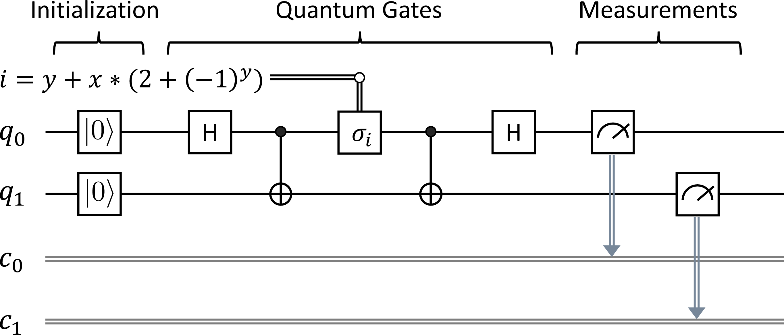
Superdense Coding (SC) introduced by Bennett & Wiesner (1992) takes advantage of entanglement in quantum mechanics to send two classical bits from Alice to Bob using just a pair of entangled qubits. Figure 2 depicts the circuit for Superdense Coding. The single wires denote qubits referred to as qi, while the double wires denote classical bits referred to as ci. Alice acts on q0 while Bob acts on q1 as follows:
-
First, q0 are q1 are initially in the basic state |0〈.〉. We need to prepare an entangled state between q0 and q1 by applying the sequence of the H gate on q0 and the CX gate on q0 and q1. The entangled state is shared between Alice and Bob using a quantum channel, where q0 and q1 are manipulated by Alice and Bob, respectively.
-
Second, Alice needs to send two classical bits x and y, where x, y ∈ {0, 1}, as depicted in Fig. 2. Depending on the values of x and y that Alice wants to send to Bob, Alice will apply the σi gate on q0, where i = y + x∗(2 + (−1)y) ranging over {0, 1, 2, 3} and σ0, σ1, σ2, and σ3 are I, X, Y, Z gates, respectively.
-
Third, we then apply the sequence of the CX gate on q0 and q1, and the H gate on q0.
-
Fourth, we measure the qubits q0 and q1, and immediately obtain two classical outcomes (0 or 1) stored in c0 and c1, respectively.
At the end, the pair (c0, c1) of classical bits obtained from Bob is expected to be the same as the pair (x, y) of classical bits sent by Alice. We would like to verify the correctness of Superdense Coding by using our symbolic model checking.
Specification of superdense coding
Regarding the actions specified in ‘Formal Specification’, we can describe the circuit for Superdense Coding with different values of classical bits used for (x, y) as follows:
-
(x, y) = (0, 0) with σ0 = I: H(0) CX(0, 1) I(0) CX(0, 1) H(0) M(0) M(1)
-
(x, y) = (0, 1) with σ1 = X: H(0) CX(0, 1) X(0) CX(0, 1) H(0) M(0) M(1)
-
(x, y) = (1, 1) with σ2 = Y: H(0) CX(0, 1) Y(0) CX(0, 1) H(0) M(0) M(1)
-
(x, y) = (1, 0) with σ3 = Z: H(0) CX(0, 1) Z(0) CX(0, 1) H(0) M(0) M(1)
Let ISC be the set of initial states for Superdense Coding. It consists of four initial states corresponding to the four possible values used for (x, y) as follows:
{(isEnd: false)
(prob: 1)
(qstate: (q[0]: |0>) (q[1]: |0>))
(bits: empty)
(actions: H(0) CX(0, 1) I(0) CX(0, 1) H(0)
            M(0) M(1))}
{(isEnd: false)
(prob: 1)
(qstate: (q[0]: |0>) (q[1]: |0>))
(bits: empty)
(actions: H(0) CX(0, 1) X(0) CX(0, 1) H(0)
            M(0) M(1))}
{(isEnd: false)
(prob: 1)
(qstate: (q[0]: |0>) (q[1]: |0>))
(bits: empty)
(actions: H(0) CX(0, 1) Y(0) CX(0, 1) H(0)
            M(0) M(1))}
{(isEnd: false)
(prob: 1)
(qstate: (q[0]: |0>) (q[1]: |0>))
(bits: empty)
(actions: H(0) CX(0, 1) Z(0) CX(0, 1) H(0)
            M(0) M(1))}
Let us refer to the four initial states as
init0
init1
init2
init3
isEnd
prob
qstate
actions 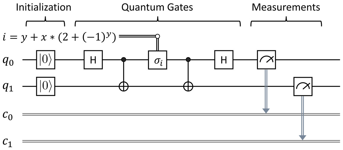
Figure 2: Superdense coding.
Model checking superdense coding
Let KSC be the Kripke structure for Superdense Coding. To model check that KSC satisfies desired properties, we specify ASC and LSC for Superdense Coding. ASC has four atomic propositions
isGateI
isGateX
isGateY
isGateZ
eq {(isEnd: true) (bits: BM) (prob: Prob) OCs} |=
    isGateI
= (Prob > 0) implies (BM[0] == 0 and BM[1] == 0) .
eq {(isEnd: true) (bits: BM) (prob: Prob) OCs} |=
    isGateX
= (Prob > 0) implies (BM[0] == 0 and BM[1] == 1) .
eq {(isEnd: true) (bits: BM) (prob: Prob) OCs} |=
    isGateY
= (Prob > 0) implies (BM[0] == 1 and BM[1] == 1) .
eq {(isEnd: true) (bits: BM) (prob: Prob) OCs} |=
    isGateZ
= (Prob > 0) implies (BM[0] == 1 and BM[1] == 0) .
eq {OCs} |= PROP = false [owise] .
where
BM
Prob The five equations say that
isGateI
(isEnd: true)
(bits: BM)
(prob: Prob)
BM[0] == 0 and BM[1] == 0
Prob > 0
gateIProp
gateXProp
gateYProp
gateZProp
<> isGateI
<> isGateX
<> isGateY
<> isGateZ
<> We model check that KSC = 〈S, ISC, T, ASC, LSC〉 satisfies
gateIProp
gateXProp
gateYProp
gateZProp
init0
init1
init2
init3
red modelCheck(init0, gateIProp) .
red modelCheck(init1, gateXProp) .
red modelCheck(init2, gateYProp) .
red modelCheck(init3, gateZProp) .
No counterexample is found in just 1 ms for each model checking experiment and so KSC satisfies
gateIProp
gateXProp
gateYProp
gateZProp Moreover, we conduct some more model checking experiments for Superdense Coding to confirm that Bob cannot receive bits that differ from the ones sent by Alice using the following commands:
red modelCheck(init0, gateXProp) .
red modelCheck(init0, gateYProp) .
red modelCheck(init0, gateZProp) .
red modelCheck(init1, gateIProp) .
red modelCheck(init1, gateYProp) .
red modelCheck(init1, gateZProp) .
red modelCheck(init2, gateIProp) .
red modelCheck(init2, gateXProp) .
red modelCheck(init2, gateZProp) .
red modelCheck(init3, gateIProp) .
red modelCheck(init3, gateXProp) .
red modelCheck(init3, gateYProp) .
where each of
init0
init1
init2
init3 Quantum teleportation
Introduction
Quantum Teleportation (QT) introduced by Bennett et al. (1993) also takes advantage of entanglement in quantum mechanics to send an unknown quantum state |ψ〈.〉 from Alice to Bob by using only three qubits and two classical bits. Because the no-cloning theorem, as stated in Wootters & Zurek (1982), does not allow copying an arbitrary unknown quantum state, the protocol becomes extremely important to transmit an arbitrary unknown quantum state from one source to another. The difference between Superdense Coding and Quantum Teleportation is that the former transmits two classical bits, while the latter transmits an arbitrary unknown quantum state.
The circuit depicted in Fig. 3 shows how the protocol works. Alice acts on q0 and q1, and Bob acts on q2 as follows:
-
First, we prepare an unknown state |ψ〈.〉 = α|0〈.〉 + β|1〈.〉 at q0, where α and β are complex numbers such that |α|2 + |β|2 = 1. Initially, q1 and q2 are in the state |0〈.〉.
-
Second, we apply a sequence of quantum gates to manipulate three qubits. In this case, we only consider the single-qubit Hadamard H and two-qubit controlled-NOT CX gates. We first apply the H gate on q1 followed by the CX gate on q1 and q2 in order to make an entangled state shared between Alice and Bob. Alice then applies the CX gate on q0 and q1 followed by the H gate on q0.
-
Third, we measure the qubits q0 and q1, and immediately obtain two classical outcomes (0 or 1) stored in c0 and c1, respectively.
-
Fourth, we conditionally apply single-qubit X and Z gates on q2 depending on the two classical bits in c0 and c1. Concretely, we use the X gate if c1 equals one and followed by the Z gate if c0 equals one.
At the end, Bob will have |ψ〈.〉 and Alice will not have it anymore. We would like to verify whether Alice can correctly send an arbitrary unknown quantum state to Bob at the end by using our symbolic model checking.
Specification of quantum teleportation
We can describe the circuit for Quantum Teleportation based on the actions specified in ‘Formal Specification’ as follows:
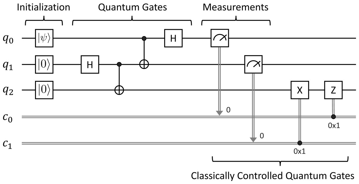
Figure 3: Quantum teleportation.
H(1) CX(1, 2) CX(0, 1) H(0) M(0) M(1) (c[1] == 1 ? X
    (2)) (c[0] == 1 ? Z(2))
Let IQT be the set of initial states for Quantum Teleportation. It consists of only one initial state as follows:
{(isEnd: false)
(prob: 1)
(qstate: (q[0]: a . |0> + b . |1>)
           (q[1]: |0>) (q[2]: |0>))
(bits: empty)
(actions: H(1) CX(1, 2) CX(0, 1) H(0)
            M(0) M(1)
            c[1] == 1 ? X(2)
            c[0] == 1 ? Z(2))}
where
a
b
isEnd
prob
qstate
actions Model checking quantum teleportation
Let KQT and
init
isSuccess
eq {(isEnd: true) (qstate: Q) (prob: Prob) OCs} |=
    isSuccess
= Prob > 0 implies (qubitAt(Q, 2) ==  qubitAt(qstate(
    init), 0) and
   qubitAt(Q, 0) =/=  qubitAt(qstate(init), 0)) .
eq {OCs} |= PROP = false [owise] .
where
Q
Prob The two equations say that
isSuccess
(isEnd: true)
(qstate: Q)
(prob: Prob)
qubitAt(Q, 2) == qubitAt(qstate(init), 0)
qubitAt(Q, 0) == qubitAt(qstate(init), 0)
Prob > 0
teleProp
<> isSuccess We want to model check that KQT = 〈S, IQT, T, AQT, LQT〉 satisfies
teleProp
init
red modelCheck(init, teleProp) . No counterexample is found in just 3 ms and so KQT satisfies
teleProp During LTL model checking, each state in a computation reachable from an initial state contains information on the probability accumulated up to the state from previous states. Ultimately, we obtain the probability of each computation. We would like to additionally check that if a computation has a probability greater than 0, the probability is also less than 1/2. We achieve this by adding the condition
Prob > 1/2
isSuccess The first equation now becomes as follows:
eq {(isEnd: true) (qstate: Q) (prob: Prob) OCs} |=
    isSuccess
= Prob > 0 implies (qubitAt(Q, 2) ==  qubitAt(qstate(
    init), 0) and
   qubitAt(Q, 0) =/=  qubitAt(qstate(init), 0) and Prob
    < 1/2) .
We then conduct the model checking experiment again and no counterexample is found because each computation indeed has the probability of 1/4 equally. This artificial model checking experiment demonstrates that we can specify quantitative properties by considering the accumulated probability across states for each computation.
Moreover, we conduct one more model checking experiment to confirm that Alice indeed keeps her initial qubit with zero probability by changing the condition
qubitAt(Q, 0) =/= qubitAt(qstate(init), 0)
qubitAt(Q, 0) == qubitAt(qstate(init), 0)
isSuccess Reachability analysis for quantum teleportation
Besides using LTL model checking, we can also use reachability analysis to verify the correctness of Quantum Teleportation with the same property mentioned above. Maude is equipped with the search command with which reachability analysis can be conducted. The following search command, where
TELEPORT
init
TELEPORT
search  in  TELEPORT: init
=>* {(qstate: Q) (isEnd: true) (prob: P) OCs}
such  that not (
   Prob > 0 implies (qubitAt(Q, 2) ==  qubitAt(qstate(
    init), 0) and
   qubitAt(Q, 0) =/=  qubitAt(qstate(init), 0))
) .
finds all states reachable from the initial state that contain
(isEnd: true)
(qstate: Q)
(prob: Prob)
isSuccess The reason why we use the Maude LTL model checker is because it is convenient to express desired properties of quantum circuits in LTL. Quantum circuits look simple but have non-determinism because of measurements, and then have multiple possible execution paths. It is necessary to take all such multiple execution paths. Desired properties of quantum circuits are in the form: for each possible execution path, something good eventually happens. For example, a qubit at the final state for each possible execution path is the same as another qubit at the initial state with a non-zero probability. Meanwhile, we need to find all states that do not satisfy the condition and we need to think in an inverse way when the search command is used. As written, we can use the search command, but because times taken by the search command (i.e., 2 ms) and the Maude LTL model checker (i.e., 3 ms) are comparable and it is convenient to express desired properties of quantum circuits in LTL, so we use the Maude LTL model checker.
Quantum secret sharing
Introduction
Quantum Secret Sharing (QSS) was first invented by Hillery, Bužek & Berthiaume (1999) and some attempts to describe quantum circuits for the protocol were presented by Joy et al. (2019). This protocol also takes advantage of entanglement to send an unknown quantum state |ψ〈.〉 from Alice to either Bob or Charlie using the mechanism of Quantum Teleportation. However, this protocol uses four qubits and three classical bits, and especially neither Bob nor Charlie can independently reconstruct |ψ〈.〉 by themselves. The one wants to retrieve the unknown quantum state |ψ〈.〉 if and only if some information from the other is provided. This protocol has been used in many applications, such as quantum money schemes introduced by Wiesner (1983), Wang et al. (2007), quantum error-correcting codes introduced by Cleve, Gottesman & Lo (1999), Matsumoto (2017), and a graph-theoretic protocol introduced by Sarvepalli (2012), Gravier et al. (2015), demonstrating its importance.
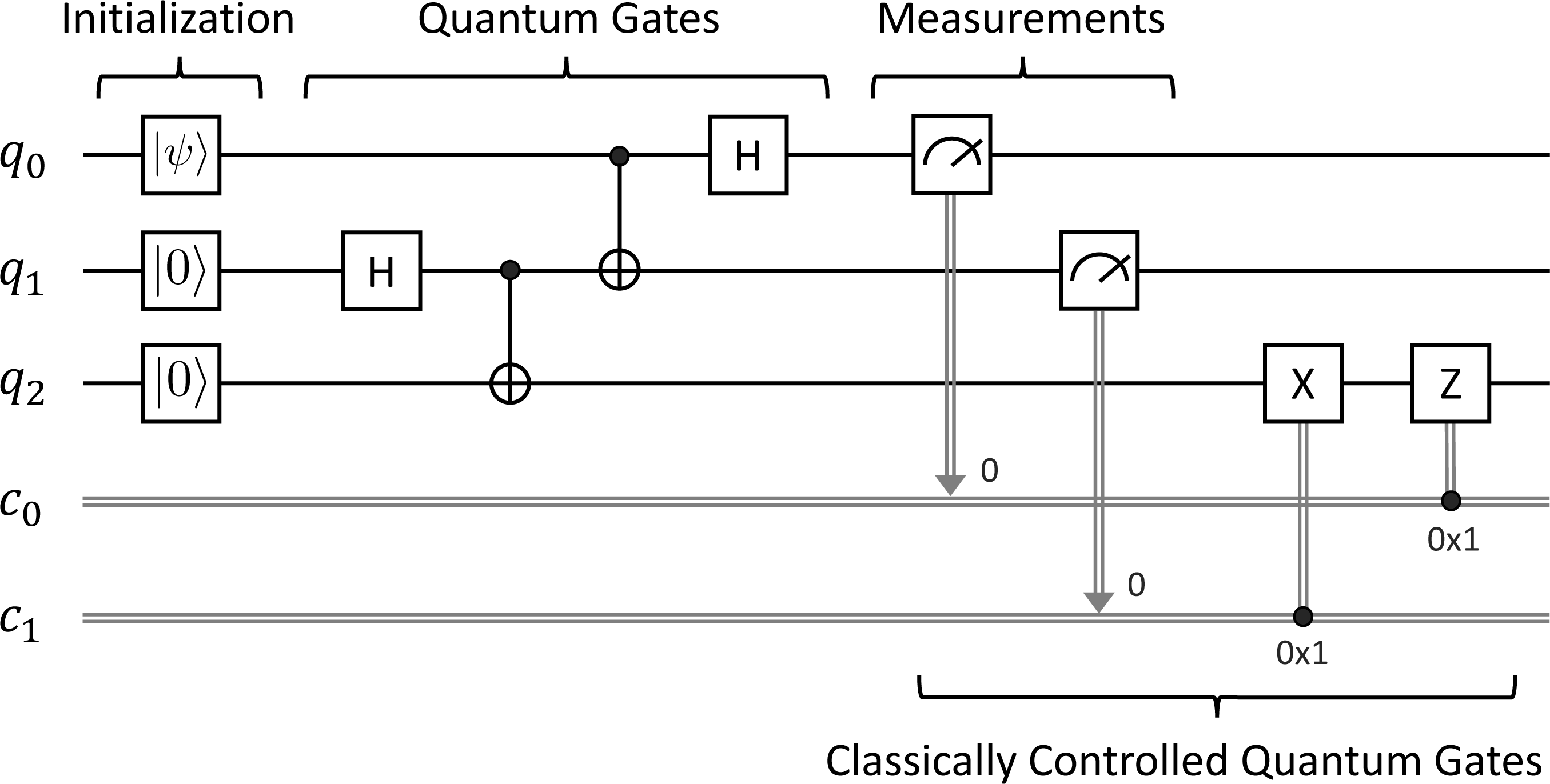
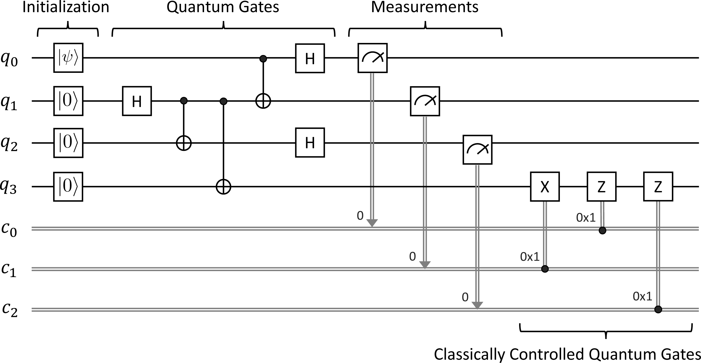
The circuit for Quantum Secret Sharing is depicted in Fig. 4. We suppose that Charlie will reconstruct the unknown quantum state |ψ〈.〉 sent by Alice with consent from Bob in the following description. Alice acts on q0 and q1, Bob acts on q2, and Charlie acts on q3 as follows:
-
First, we prepare an arbitrary unknown state |ψ〈.〉 = α|0〈.〉 + β|1〈.〉 at q0, where α and β are complex numbers such that |α|2 + |β|2 = 1. Initially, q1, q2, and q3 are in the basic state |0〈.〉.
-
Second, we apply a sequence of quantum gates to manipulate four qubits. We first apply the H gate on q1, the CX gate on q1 and q2, and the CX gate on q1 and q3 in order to make an entangled state shared between Alice, Bob, and Charlie. Alice then applies the CX gate on q0 and q1 followed by the H gate on q0. Bob then applies the H gate on q2 to make it possible to measure in X-basis (or the diagonal basis {| + 〈.〉, | − 〈.〉}) subsequently.
-
Third, we measure the qubits q0, q1, and q2 and immediately obtain three classical outcomes (0 or 1) stored in c0, c1, and c2, respectively.
-
Fourth, we conditionally apply single-qubit X, Z, and Z gates on q3 depending on the three classical bits in c1, c0, and c2. Concretely, we use the X gate if c1 equals one and similarly for others. We can see that Charlie also needs to use the measurement outcome from Bob in order to reconstruct |ψ〈.〉 in this step.
At the end, Charlie will have |ψ〈.〉 with consent from Bob, and Alice will not have it anymore. We would like to verify whether Charlie can correctly reconstruct an arbitrary unknown quantum state sent by Alice with consent from Bob at the end by using our symbolic model checking. Note that this property is one aspect of QSS because we do not consider the following property under verification: neither Bob nor Charlie can independently reconstruct |ψ〈.〉 by themselves.
Specification of quantum secret sharing
We can describe the circuit for Quantum Secret Sharing based on the actions specified in ‘Formal Specification’ as follows:
Figure 4: Quantum secret sharing.
H(1) CX(1, 2) CX(1, 3) CX(0, 1) H(0) H(2) M(0) M(1) M
    (2)
(c[1] == 1 ? X(3)) (c[0] == 1 ? Z(3)) (c[2] == 1 ? Z
    (3))
Let IQSS be the set of initial states for Quantum Secret Sharing. It consists of only one initial state as follows:
{(isEnd: false)
(prob: 1)
(qstate: (q[0]: a . |0> + b . |1>)
           (q[1]: |0>) (q[2]: |0>) (q[3]: |0>))
(bits: empty)
(actions:
    H(1) CX(1, 2) CX(1, 3) CX(0, 1) H(0) H(2)
    M(0) M(1) M(2)
    c[1] == 1 ? X(3)
    c[0] == 1 ? Z(3)
    c[2] == 1 ? Z(3))}
where
a
b
isEnd
prob
qstate
actions Model checking quantum secret sharing
Let KQSS and
init
isSuccess
eq {(isEnd: true) (qstate: Q) (prob: Prob) OCs} |=
    isSuccess
= Prob > 0 implies (qubitAt(Q, 3) ==  qubitAt(qstate(
    init), 0) or
                        (-1) . qubitAt(Q, 3) ==  qubitAt(
    qstate(init), 0)).
eq {OCs} |= PROP = false [owise] .
where
Q
Prob The two equations say that
isSuccess
(isEnd: true)
(qstate: Q)
(prob: Prob)
qubitAt(Q, 3) == qubitAt(qstate(init), 0)
qubitAt(Q, 3) == qubitAt(qstate(init), 0)
Prob > 0
(-1). qubitAt(Q, 3) == qubitAt(qstate(init), 0)
qubitAt(Q, 3) == qubitAt(qstate(init), 0)
secretProp
<> isSuccess We want to model check that KQSS = 〈S, IQSS, T, AQSS, LQSS〉 satisfies
secretProp
init
red modelCheck(init, secretProp) . No counterexample is found in just 13 ms and so KQSS satisfies
secretProp Quantum gate teleportation
Introduction
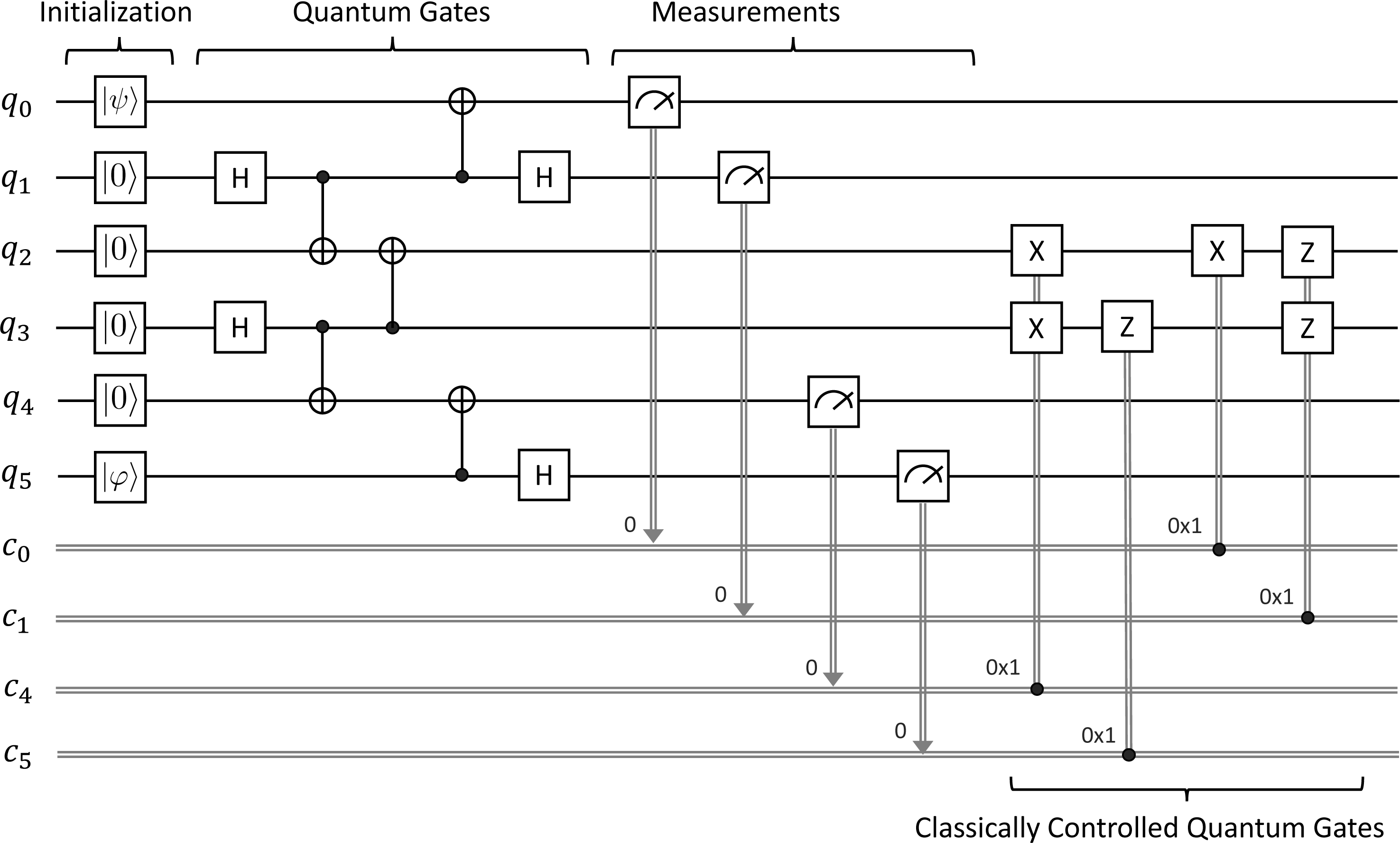
Quantum Gate Teleportation (QGT) is a generalization of quantum teleportation invented by Gottesman & Chuang (1999) for teleporting two arbitrary states through the controlled-NOT gate with the use of six qubits and four classical bits. This protocol can be regarded as a single technique to reduce resource requirements for quantum computers and unifies known protocols for fault-tolerant quantum computations, demonstrating its importance.
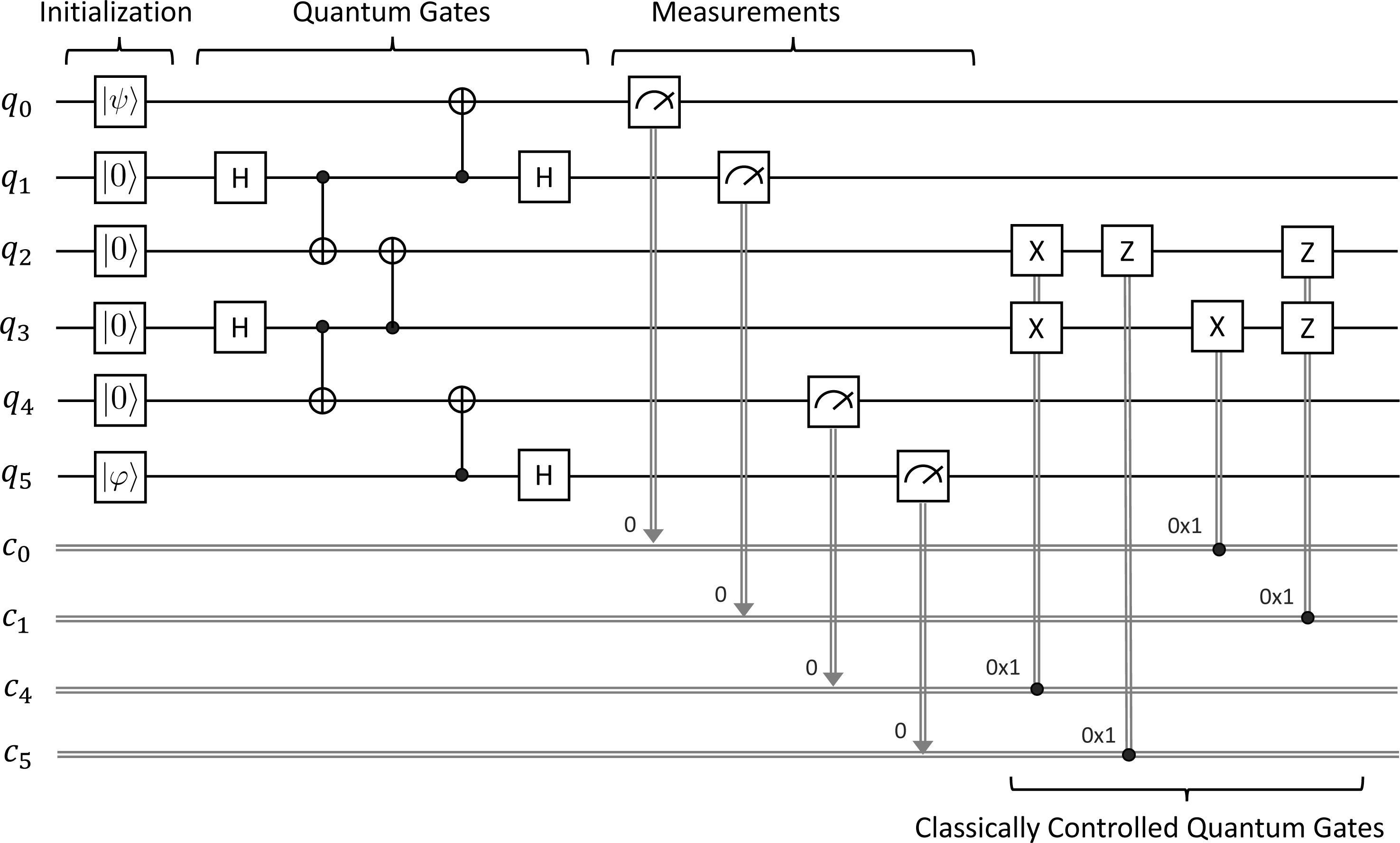
The circuit for Quantum Gate Teleportation2 is depicted in Fig. 5. Alice acts on q0 and q1, Bob acts on q2, q3, q4, and q5 as follows:
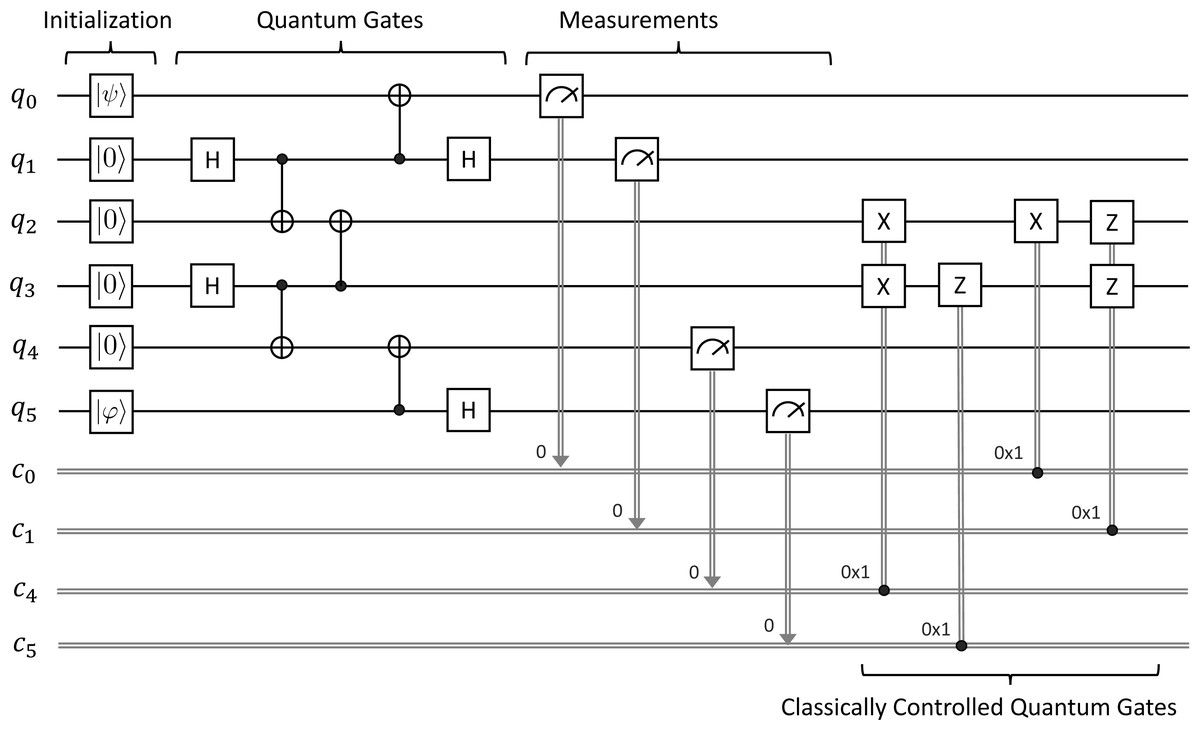
Figure 5: Quantum gate teleportation.
-
First, Alice prepares an arbitrary unknown state |ψ〈.〉 = a|0〈.〉 + b|1〈.〉 at q0, where a and b are complex numbers such that |a|2 + |b|2 = 1. Similarly, Bob also prepares an arbitrary unknown state |φ〈.〉 = c|0〈.〉 + d|1〈.〉 at q5. Initially, q1, q2, q3, and q4 are in the basic state |0〈.〉.
-
Second, we prepare an entangled state shared between Alice and Bob from q1 to q4 by applying a sequence of quantum gates as follows. We first apply the H gate on q1, the CX gate on q1 and q2, the H gate on q3, the CX gate on q3 and q4, and finally the CX gate on q3 and q2.
-
Third, Alice then applies the CX gate on q1 and q0 followed by the H gate on q1. Meanwhile, Bob applies the CX gate on q5 and q4 followed by the H gate on q5.
-
Fourth, we measure the qubits q0, q1, q4, and q5 and immediately obtain four classical outcomes (0 or 1) stored in c0, c1, c4, and c5, respectively.
-
Fifth, we conditionally apply the X gate on q2 and q3, the Z gate on q3, the X gate on q2, and the Z gate on q2 and q3, depending on the four classical bits in c4, c5, c0, and c1.
At the end, Bob will have the controlled-NOT gate of |φ〈.〉 and |ψ〈.〉 (i.e., CX(|φ〈.〉, |ψ〈.〉) at the indices q2 and q3. We would like to verify whether Alice can successfully teleport two arbitrary unknown quantum states through the controlled-NOT gate to Bob at q2 and q3 at the end by using our symbolic model checking.
Specification of quantum gate teleportation
We can describe the circuit for Quantum Gate Teleportation based on the actions specified in ‘Formal Specification’ as follows:
H(1) CX(1, 2) H(3) CX(3, 4) CX(3, 2) CX(1, 0) H(1) CX
    (5, 4) H(5)
M(0) M(1) M(4) M(5)
(c[4] == 1 ? X(2) X(3))
(c[5] == 1 ? Z(3))
(c[0] == 1 ? X(2))
(c[1] == 1 ? Z(2) Z(3))
Let IQGT be the set of initial states for Quantum Gate Teleportation. It consists of only one initial state as follows:
{(isEnd: false)
(prob: 1)
(qstate: (q[0]: a . |0> + b . |1>)
           (q[1]: |0>) (q[2]: |0>)
           (q[3]: |0>) (q[4]: |0>)
           (q[5]: c . |0> + d . |1>))
(bits: empty)
(actions:
    H(1) CX(1, 2) H(3) CX(3, 4) CX(3, 2) CX(1, 0) H(1)
    CX(5, 4) H(5)
    M(0) M(1) M(4) M(5)
    (c[4] == 1 ? X(2) X(3))
    (c[5] == 1 ? Z(3))
    (c[0] == 1 ? X(2))
    (c[1] == 1 ? Z(2) Z(3))}
where
a
b
c
d
isEnd
prob
qstate
actions Model checking quantum gate teleportation
Let KQGT and
init
isSuccess
eq {(isEnd: true) (qstate: Q) (prob: Prob) OCs} |=
    isSuccess
= Prob > 0 implies (qubitAt(Q, 3 2) ==  qubitAt(
    targetQState, 0 1) or
                        (-1) . qubitAt(Q, 3 2) ==  qubitAt(
    targetQState, 0 1)) .
eq {OCs} |= PROP = false [owise] .
where
Q
Prob
targetQState
eq targetQState = ((q[0]: c . |0> + d . |1>) (q[1]: a
    . |0> + b . |1>)).CX(0, 1) .
The two equations to specify AQGT say that
isSuccess
(isEnd: true)
(qstate: Q)
(prob: Prob)
qubitAt(Q, 3 2) == qubitAt(targetQState, 0 1)
(-1) . qubitAt(Q, 3 2) == qubitAt(target
QState, 0 1)
Prob > 0
(-1) . qubitAt(Q, 3 2) == qubitAt(targetQState, 0 1)
qubitAt(Q, 3 2) == qubitAt(targetQState, 0 1)
gateProp
<> isSuccess We want to model check that KQGT = 〈S, IQGT, T, AQGT, LQGT〉 satisfies
gateProp
init
red modelCheck(init, gateProp) . No counterexample is found in just 176 ms and so KQGT satisfies
gateProp Remark on Quantum Gate Teleportation
This section describes a remark on Quantum Gate Teleportation where we show that a circuit for the original version of the protocol does not satisfy its desired property, while we present a revised circuit for the protocol and verify that it satisfies its desired property using our symbolic model checking approach.
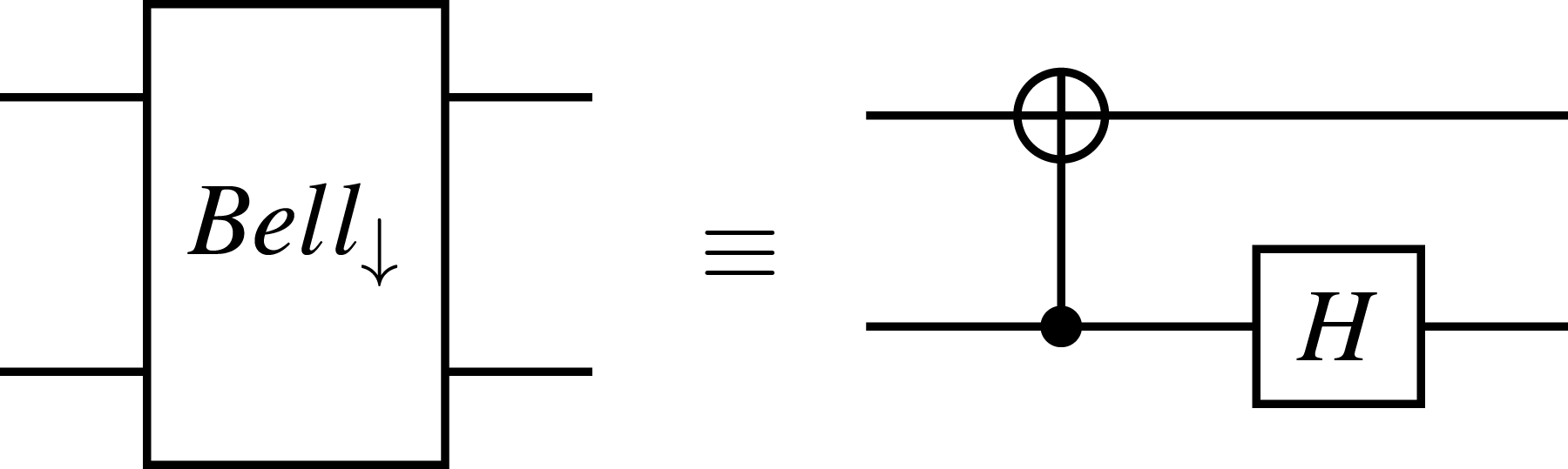
The reader can refer to the circuit for the original version of Quantum Gate Teleportation from Gottesman & Chuang (1999), Fig. 2. In that figure, they use a Bell measurement denoted by the box B twice in the circuit. A Bell measurement can be described in terms of a CX gate, a Hadamard gate, and a measurement in the standard basis. However, there are two possible orientations for applying the CX gate and the Hadamard gate. The difference is apparent by comparing Figs. 6 and 7 as also presented by Williams (2008). The Bell measurement that uses the Bell-basis measurement gate in Fig. 6 is called the up Bell measurement. Meanwhile, the Bell measurement that uses the Bell-basis measurement gate inserted upside down in Fig. 7 is called the down Bell measurement. Gottesman & Chuang (1999) did not explicitly clarify which Bell measurement was used. However, they described it in their article exactly as follows:
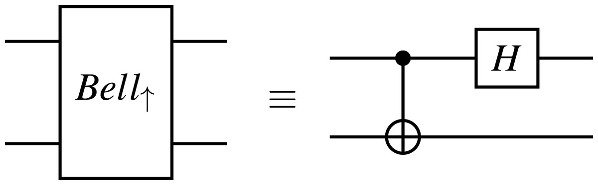
Figure 6: A Bell-basis measurement gate.
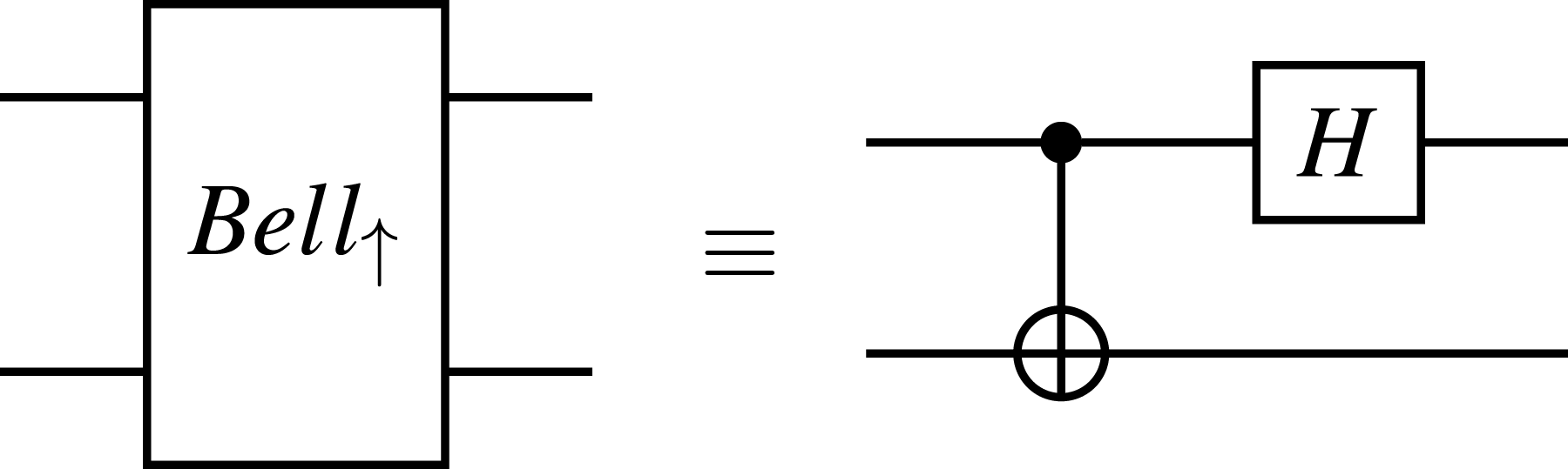
The box B represents measurement in the Bell basis; that is, if the two qubits entering B are found to be |00〈.〉 + |11〈.〉 (leaving out the normalization for clarity), then the outputs xy = 00; for |01〈.〉 + |10〈.〉, xy = 10; for |00〈.〉 − |11〈.〉, xy = 01; and for |01〈.〉 − |10〈.〉, xy = 11.
Note that xy denotes the first and second qubits entering the box B. Based on the above description in the original article, we use the down Bell measurement. If so, the circuit for Quantum Gate Teleportation is depicted in Fig. 8. Let us call this circuit the original circuit.
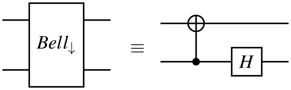
Figure 7: A Bell-basis measurement gate inserted upside down.
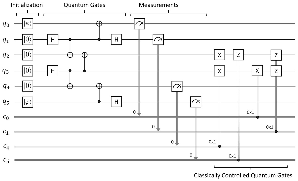
Figure 8: A possible circuit for Quantum Gate Teleportation based on the description from Gottesman & Chuang (1999).
We conducted a model checking experiment with the same initial state and the desired property described in ‘Quantum Gate Teleportation’ for the original circuit. A counterexample was found by the Maude LTL model checker, implying that Quantum Gate Teleportation does not satisfy the property with the use of the original circuit. Because the counterexample is overlong, we just excerpt and present the final state repeated forever in the counterexample as follows:
{(isEnd: true)
(prob: 1/16)
(qstate:
    (q[0]: |0>) (q[1]: |0>)
    (q[4]: |0>) (q[5]: |1>)
    (q[3 2]: (a .* c) . |0> (x) |0> + (a .* d) . |1> (x
    ) |1> +
               (b .* c .*  -1) . |0> (x) |1> + (b .* d .*
    -1) . |1> (x) |0>)
(bits: (0 |-> 0, 1 |-> 0, 4 |-> 0, 5 |-> 1))
(actions: nil)
We can see that the qubits at indices 3 and 2 do not match the controlled-NOT gate of the two arbitrary states represented by
targetQState We revised the original circuit for Quantum Gate Teleportation by changing the positions of the Z and X gates applied to qubits with respect to the values of c5 and c0, respectively. Concretely, we apply the Z gate to q3 instead of q2, the X gate to q2 instead of q3 depending on the values of c5 and c0, respectively, for the revised circuit compared to the original circuit. The revised circuit is depicted in Fig. 5 in ‘Quantum Gate Teleportation (QGT)’. For the revised circuit of Quantum Gate Teleportation, we successfully verified the correctness of the protocol by using our symbolic model checking approach. This demonstrates the usefulness of our symbolic model checking approach for verifying quantum circuits.
Experimental Results
This section summarizes our experimental results for verifying the correctness of several quantum communication protocols with our symbolic model checking approach, including Superdense Coding introduced by Bennett & Wiesner (1992), Quantum Teleportation introduced by Bennett et al. (1993), Quantum Secret Sharing introduced by Hillery, Bužek & Berthiaume (1999), Entanglement Swapping introduced by Zukowski et al. (1993), Quantum Gate Teleportation introduced by Gottesman & Chuang (1999), Two Mirror-image Teleportation introduced by Williams (2008), and Quantum Network Coding introduced by Satoh, Gall & Imai (2012). The experiments were conducted with an iMac that carries a 4 GHz microprocessor with eight cores and 32 GB memory of RAM. The experimental results are shown in Table 3. The second, third, and fourth columns denote the number of qubits in each protocol, the number of states in the reachable state space of each protocol under model checking, and the verification time for each protocol, respectively.
For case studies ranging from two to ten qubits, model checking experiments were quickly completed in times from 1 ms to 2,446 ms as shown in Table 3. The number of states in the reachable state space for Quantum Network Coding with ten qubits is notably larger compared to the number of states in the reachable state space for each of the first six protocols. Nevertheless, the model checking experiment for Quantum Networking Coding could be completed in a short amount of time. Without the aid of computer programs, such as our support tool implemented in Maude, it is almost impossible to achieve the same results. These results demonstrate the usefulness of our symbolic model checking approach to verifying quantum circuits in Maude. As one piece of future work, we would like to tackle more case studies with a larger number of qubits to present the scalability of our approach.
| Protocol | Qubits | States | Verification time |
|---|---|---|---|
| Superdense coding | 2 | 16 | 1 ms |
| Quantum teleportation | 3 | 27 | 3 ms |
| Quantum secret sharing | 4 | 65 | 13 ms |
| Entanglement swapping | 4 | 29 | 3 ms |
| Two mirror-image teleportation | 6 | 151 | 15 ms |
| Quantum gate teleportation | 6 | 168 | 176 ms |
| Quantum network coding | 10 | 7,373 | 2,446 ms |
Discussion
This section discusses some limitations of our approach, challenges in using a classical model checker to verify quantum circuits with their desired properties, and how we address these challenges.
Limitations
In the context of symbolic reasoning for complex numbers, we have extended rational numbers supported in Maude to deal with complex numbers. Our objective is to represent arbitrary complex numbers in a pure quantum state using fresh constants representing arbitrary complex numbers and manipulating them without using any concrete values for real numbers. As a result, our current framework cannot handle any concrete values for real numbers. Nevertheless, we plan to explore the use of float numbers supported in Maude for simulating quantum circuits with concrete values in the future. As shown in Appendix 2, we have specified some basic operations for complex numbers, such as multiplication, division, addition, conjugation, absolute, power, and square roots. Note that the formal specification of complex numbers is not complete in this article. Hence, there may be some cases where symbolic reasoning for complex numbers could not further reduce terms. As part of our future work, we aim to enrich the framework for complex number reasoning as much as possible.
Regarding symbolic reasoning for quantum computation, we only support a limited set of quantum gates, including I, X, Y, Z, H, CX, S, T, CY, CZ, SWAP, CCY, CCZ, and CSWAP gates. Consequently, a restricted set of quantum protocols can be described in our framework. Although we support a universal set of quantum gates, including the Clifford gates (i.e., H, S, and CX) and the phase shift gate T, universal quantum computations could not be handled by our framework at this moment because the symbolic reasoning for complex numbers is not complete. We would like to extend our symbolic reasoning to handle more quantum gates so that a wider range of quantum protocols can be verified using our approach.
Challenges and future prospects
There are some challenges that we need to address in order to use the Maude LTL model checker, a classical model checker, to verify quantum circuits with their desired properties. In addition, this section also outlines future prospects in model checking quantum circuits.
-
First, we need to devise a way to specify quantum states, quantum gates, and measurements in a Maude specification to reason about quantum computation. We specified quantum states, quantum gates, and measurements in Dirac notation and used a set of laws from quantum mechanics and basic matrix operations to reason about quantum computation automatically in Maude. Moreover, Maude does not support complex numbers as a built-in type. Therefore, we extended rational numbers, a built-in type in Maude, so as to deal with complex numbers symbolically as described in Appendix A.
-
Second, quantum gates can be applied to quantum states in a deterministic way, while quantum measurements are inherently non-deterministic and the states after the measurements will collapse. It is natural to use rewriting logic to describe non-deterministic or concurrent behaviors in Maude in the form of rewrite rules. We specified a binary projective measurement using two rewrite rules corresponding to two non-deterministic choices, as described in ‘Formal Specification’.
-
Third, we need to appropriately handle both pure and entangled states in our formal specification and devise a simple notation to conveniently describe the behavior of quantum circuits. We specified a whole quantum state as a collection of qubits associated with indices in quantum circuits, enabling flexible reference to specific parts of a quantum state using indices. The behavior of quantum circuits has been specified as a list of actions, a convenient and sufficient approach for us to concisely describe their behavior.
-
Lastly, we need to represent quantum states and quantum gates in order to effectively model check quantum circuits with as many qubits as possible. Using Dirac notation in our specification allows us to avoid many redundancies compared to explicitly using vectors and matrices to represent quantum states and quantum gates, respectively, making our representation more compact than that of Paykin, Rand & Zdancewic (2017). Early work proposed by Gay, Nagarajan & Papanikolaou (2005) could not support the analysis of quantum systems with five qubits, while our approach could handle case studies of up to ten qubits, showing the effectiveness of our approach. However, in order to handle quantum systems with hundreds of qubits in the future, we need to use or come up with advanced techniques to effectively simulate quantum computation(e.g., using decision diagrams for quantum computing proposed by Wille, Hillmich & Burgholzer (2022), Wille, Hillmich & Burgholzer (2023)) or analyze such quantum systems in a modular way.
Last but not least, our approach implemented in Maude can be a first step toward a general framework for specifying and verifying quantum circuits when we can reuse some essential elements in the Kripke structures. For specifying and verifying a quantum circuit, we are supposed to define an initial state, describe the behavior of the quantum circuit in terms of a list of actions, and specify atomic propositions and the labeling function based on which a desired property can be constructed. Given the system specification with the initial state and the desired property, the Maude LTL model checker automatically checks whether the system specification satisfies the desired property reachable from the initial state.
Related Work
There are several studies in the early work of formal specification and verification of quantum protocols, such as Gay, Nagarajan & Papanikolaou (2005); Elboukhari, Azizi & Azizi (2010). For example, Gay, Nagarajan & Papanikolaou (2005) provide a way to use classical model checkers (e.g., PRISM - a probabilistic model checker) to analyze quantum protocols. They give each quantum state a unique number and the transition from a unique number to another unique number models the action of quantum gates and measurements. Their approach needs to enumerate states, calculate the state transitions in advance, and then encode them into a PRISM specification. Although they developed a so-called PRISMGEN tool to automate this, their approach is impractical in reality and only supports two or three qubits because of the exponential growth of the number of states. Our approach does not need to enumerate such states in advance because a quantum state is directly specified in Dirac notation with scalars. Moreover, rewrite rules are used to specify the action of quantum gates and measurements, making our approach feasible to deal with more qubits. For example, we have verified the correctness of Quantum Network Coding that has ten qubits by using our symbolic model checking approach.
Ying (2021) proposes a framework for assertion-based verification of quantum circuits by using model checking techniques. In this work, quantum circuits are represented by tensor networks, where a tensor is a multi-dimensional array of complex numbers, and two tensors sharing indices are connected by a tensor contraction, which basically is matrix calculation. Quantum states and quantum gates are specified as tensors, and quantum circuits are specified as tensor networks. Given a quantum state as an input to a quantum circuit, the output will be the contraction of the quantum state and the quantum circuit. Assertions or properties about quantum circuits are specified using computation tree quantum logic (CTQL), an extension of the Birkoff-von Neumann quantum logic presented in Birkhoff & Neumann (1936). Using tensor network representation of quantum circuits, they can conveniently implement a reachability analysis algorithm and a model checking algorithm for quantum circuits by contraction of tensor networks. Compared to our work, Dirac notation is used to express quantum states and quantum gates instead of tensors, and quantum circuits are described by an action list with simple notations instead of tensor networks. Our reasoning on quantum circuits is mainly based on the laws of quantum mechanics and matrix operations with Dirac notation, but they construct contraction between tensors in tensor networks. We use LTL to express desired properties for quantum circuits instead of CTQL. It seems that they cannot deal with quantum circuits together with the appearance of classical bits obtained from measurements, while our approach can do so. Moreover, they do not show any case study to which their framework can apply.
Burgholzer & Wille (2021) have proposed an advanced method for equivalence checking of quantum circuits. Their approach involves two quantum circuits G and G′ as inputs and they check whether the two quantum circuits are equivalent. They leverage two key observations: (1) quantum circuits are inherently reversible, and (2) even small differences in quantum circuits may impact the overall behavior of quantum circuits. Let us suppose that two quantum circuits are sequences of unitary transformations: G = Um−1…U0 = U and operating on n qubits. Executing a quantum circuit to evolve an initial state |ψ〈.〉 to another state |ψ′〈.〉 such that Um…U0|ψ〈.〉 = U|ψ〈.〉 = |ψ′〈.〉 is called simulation. For (1), G is equivalent to G′ if and only if or when due to their unitary matrices. They employ decision diagrams to represent matrices and try to resolve into the identity matrix I for effectively solving the equivalence checking problem. For (2), comparing the entire matrices of U and U′ is unnecessary when two quantum circuits are not equivalent. Comparing some columns of each U and U′ is enough to conclude the equivalence checking problem. Constructing a single column of U (or U′) equates to simulating G (or G′) with the standard basis state |i〈.〉 as follows: , for j ∈ {1, …, m − 1}. As the results of these simulations, if and are different, it indicates non-equivalence of the two quantum circuits. These can be quickly checked through a randomized selection of some columns with simulations. While their approach is promising, it differs from ours when we take a formal specification for a quantum circuit and a formal property for a desired property as inputs and check whether the quantum circuit satisfies the desired property. Nevertheless, we may utilize their idea to extend our symbolic reasoning to check the equivalence of quantum circuits, which would be one interesting direction.
The ZX calculus, as proposed by Coecke & Duncan (2011), is a graphical formal language for quantum systems equipped with a robust set of rewrite rules that enable a graphical rewriting system for quantum computation. The graphical formalism of the ZX calculus can be implemented in the automated rewriting system Quantomatic proposed by Kissinger & Zamdzhiev (2015) for the automatic simplification process. The ZX calculus has various applications in quantum computing, such as verifying quantum error-correcting codes and equivalence checking of quantum circuits. For example, Peham, Burgholzer & Wille (2022) proposed an approach to the equivalence checking of quantum circuits using the ZX calculus. Given two quantum circuits U and U′, they produce their corresponding representations as ZX-diagrams D and D′. These diagrams are then combined into D†D′ and simplified using the set of rewrite rules. If the result is in the form of the identity diagram, they can conclude their equivalence. Otherwise, nothing can be concluded because there are multiple forms for a ZX diagram in general. This approach is intuitive when we can see which rewrite rules are used and how ZX diagrams are changed accordingly. Our approach based on Dirac notation may be less intuitive. However, our approach is to verify whether quantum circuits satisfy their desired properties, which are different from the equivalence checking of quantum circuits as mentioned above.
Rand, Paykin & Zdancewic (2018) implement the QWIRE programming language, a high-level abstraction to describe quantum circuits for programmers, in the Coq proof assistant and use Coq’s theorem proving features to prove desired properties for quantum circuits. They explicitly use matrix representations, while we use Dirac notation to reason about quantum circuits. As the inherent problem of theorem proving, they need to provide necessary lemmas in order to prove some properties that can be considered the most challenging task in theorem proving. Our approach is model checking and so it is completely automatic.
Our symbolic approach to model checking quantum circuits is inspired by Shi et al. (2021) and so it is the closest work to ours. However, their approach is oriented to theorem proving, not model checking. They also use Dirac notation with a small set of laws to specify quantum states, quantum gates, measurements, and reasoning about quantum circuits in Coq, an interactive theorem prover. However, they usually require human users to provide necessary lemmas to complete their proofs, which is generally a challenging task. Meanwhile, our approach is fully automatic and requires no human intervention. Moreover, our implementation can be a first step toward a general framework to formally specify and verify quantum circuits in a symbolic way in Maude.
Conclusion
We have proposed a symbolic approach to model checking quantum circuits using a set of laws from quantum mechanics and basic matrix operations with Dirac notation. We have analyzed the correctness of several quantum communication protocols in the early stage of quantum communication: Superdense Coding, Quantum Teleportation, Quantum Secret Sharing, Entanglement Swapping, Quantum Gate Teleportation, Two Mirror-image Teleportation, and Quantum Network Coding as case studies to demonstrate the usefulness of our approach. In particular, we have identified that the original version of Quantum Gate Teleportation did not satisfy its desired property, and have proposed a revised version and confirmed its correctness using our approach and support tool. Moreover, our implementation developed in Maude can be a first step toward a general framework to formally specify and verify quantum circuits using our symbolic model checking approach. Our specification considers the probabilities of measurements, and then we can tackle both qualitative and quantitative properties with the built-in LTL model checker in Maude.
As one piece of our future work, we would like to extend our symbolic reasoning to handle more quantum gates and more complicated reasoning on complex number operations. As usual, we need to conduct more case studies to demonstrate the usefulness of our approach/implementation. As another line of future work, we also would like to apply our symbolic approach to model checking quantum programs and quantum cryptography protocols.