
Aerosols chemical composition, light extinction, and source apportionment near a desert margin city, Yulin, China
- Published
- Accepted
- Received
- Academic Editor
- Xinfeng Wang
- Subject Areas
- Atmospheric Chemistry, Environmental Impacts
- Keywords
- PM10/PM2.5, Chemical species, Light extinction, Potential contribution source function, Principal component analysis, Yulin
- Copyright
- © 2020 Lei et al.
- Licence
- This is an open access article distributed under the terms of the Creative Commons Attribution License, which permits unrestricted use, distribution, reproduction and adaptation in any medium and for any purpose provided that it is properly attributed. For attribution, the original author(s), title, publication source (PeerJ) and either DOI or URL of the article must be cited.
- Cite this article
- 2020. Aerosols chemical composition, light extinction, and source apportionment near a desert margin city, Yulin, China. PeerJ 8:e8447 https://doi.org/10.7717/peerj.8447
Abstract
Daily PM10and PM2.5 sampling was conducted during four seasons from December 2013 to October 2014 at three monitoring sites over Yulin, a desert margin city. PM10 and PM2.5 levels, water soluble ions, organic carbon (OC), and elemental carbon (EC) were also analyzed to characterize their chemical profiles. bext (light extinction coefficient) was calculated, which showed the highest in winter with an average of 232.95 ± 154.88 Mm−1, followed by autumn, summer, spring. Light extinction source apportionment results investigated (NH4)2SO4 and NH4NO3 played key roles in the light extinction under high RH conditions during summer and winter. Sulfate, nitrate and Ca2 + dominated in PM10/PM2.5 ions. Ion balance results illustrated that PM samples were alkaline, and PM10 samples were more alkaline than PM2.5. High SO42−/K+ and Cl−/K+ ratio indicated the important contribution of coal combustion, which was consistent with the OC/EC regression equation intercepts results. Principal component analysis (PCA) analyses results showed that the fugitive dust was the most major source of PM, followed by coal combustion & gasoline vehicle emissions, secondary formation and diesel vehicle emissions. Potential contribution source function (PSCF) results suggested that local emissions, as well as certain regional transport from northwesterly and southerly areas contributed to PM2.5 loadings during the whole year. Local government should take some measures to reduce the PM levels.
Introduction
Atmospheric aerosols have been found to be associated with adverse influences on atmospheric visibility, human health, and global climate change (Watson, 2002; Yuan et al., 2006; Cao et al., 2009; Huang et al., 2014). Aerosol extinction (scattering and absorption) plays the key role in the earth system (such as, radiative balance and energy budget) (Charlson et al., 1992). Chemical components of PM contributed to extinction can establish control measurement to alleviate visibility degradation (Tao et al., 2015). Sulfate, nitrate, organic matter (OM) and elemental carbon (EC) have been considered as dominant components of PM (Cao et al., 2003; Shen et al., 2014). All of the chemical compounds contributed to visibility degradation (Lee et al., 2009).
Yulin (36.95°−39.58°N, 107.46°−111.25°E), located in the Mu Us Desert, is one of the Asian Pacific Regional Aerosol Characterization Experiment (ACE-Asia) super site. However, most studies carried in Yulin have been studied to determine the chemical and physical profiles of Asian dust and its transportation (Xu et al., 2004). As the national energy and chemical industrial base, fossil fuel consumption and motor vehicles have rapidly increased in Yulin because of the economic growth, population expansion and urbanization. Actually, a study has been conducted recently aiming to understand brown carbon (BrC) can be also emitted from coal combustion in Yulin (Lei et al., 2018). However, seasonal PM levels, chemical species and visibility degradation are still lacking. It is not known dominant chemical components to light extinction during different seasons. Such information will offer practical and significant values in making relevant control to increase the atmospheric visibility. In this study, PM sampling was conducted in three represented sites for one year, and water-soluble ions and carbonaceous species (OC/EC) were also measured to understand PM pollution and their potential sources.
Materials & Methods
Sample collection
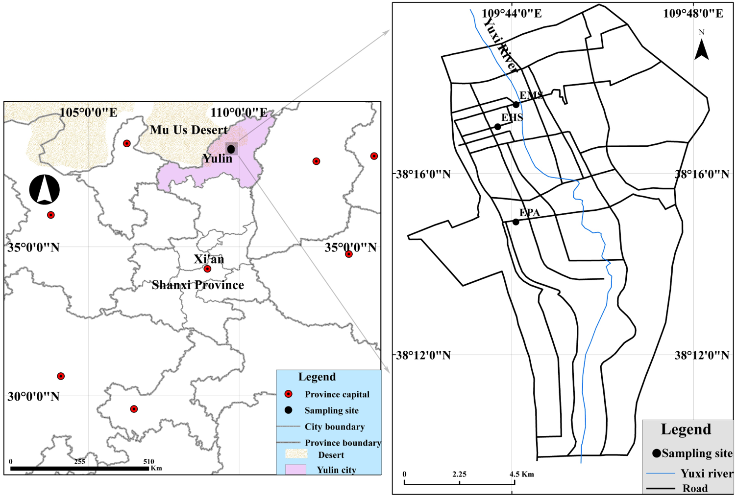
Samplings were conducted at three sites (Fig. 1): Environmental Monitoring Station (EMS) is a mixed commercial-residential-traffic site; Experimental High School (EHS) represents a residential site, and Environmental Protection Agency (EPA) is considered as rural areas. All the sampling sites have been permitted and coordinated by the Yulin Environmental Monitoring Station. We selected four months for each season which were winter (December 2013), spring (April 2014), summer (July 2014), October (autumn 2014). PM samples were collected by six mini-volume samplers (Airmetrics, Springfield, OR) at 5 L min−1. Table S1 listed the sampling information about characteristics of the PM fraction sampling measurements. 121 PM10 and 285 PM2.5 samples were collected onto 47-mm quartz microfiber filters (Whatman, Maidstone, UK) using six minivolume samplers (Airmetrics, Springfield, OR) at 5 L/min. Before sampling, the quartz filters were pre-heated to 800 °C for 3 h to remove any residual carbon. After sampling, the filters were placed in clean plastic cassettes and stored in a refrigerator at ∼4 °C until in order to minimize the evaporation of volatile components. More details can be found in Lei et al. (2018).
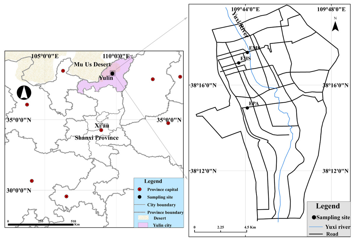
Figure 1: Locations of the monitoring sites and surrounding region.
Mass and chemical analysis
PM samples were equilibrated using controlled temperature (20–23 °C) and relative humidity (35–45%) desiccators for 24 h before and after sampling, and their mass loadings were determined gravimetrically using a Sartorius MC5 electronic microbalance (±1 µg sensitivity; Sartorius, Göttingen, Germany). Each filter was weighed at least three times before and after sampling after 24 h equilibration period. The differences among the three repeated weightings typically were less than 10 µg for blanks and 15 µg for sample filters. 1/4 of each filter sample was extracted by 10 mL distilled-deionized water (18.2 M Ω) to analyze ions. Cations were detected by a CS12A column (Dionex Co., Sunnyvale, CA) and 20 mM methanesulfonate as an eluent. Anions were separated by an AS11-HC column (Dionex Co., Sunnyvale, CA) using 20 mM KOH as the eluent with detection limits less than 0.05 mg/L (Chow & Watson, 1999). Standard reference materials produced by the National Research Center for Certified Reference Materials, China, were analyzed for quality assurance purposes. Blank values were subtracted from sample concentrations. One sample in each group of ten samples was selected to analyze twice for quality control purposes. Additional details of ions analysis can be found in Shen et al. (2008). OC and EC were analyzed using DRI Model 2001 Thermal/Optical Carbon Analyzer (Atmoslytic Inc., Calabasas, CA, USA) based on the thermal/optical reflectance (TOR) method (Chow et al., 2007). The analyzer was calibrated with CH4 daily. One replicate analysis was performed for each of 10 samples.
Data analysis
Neutralization factor
The neutralization factor (NF) can be used to describe the interaction between cations and anions (Shen et al., 2012). The NF of NH4+, Ca2+, Mg2+ have been calculated using the formula below (1)
Where X may be NH4+, Ca2+ or Mg2+, using their equivalent concentrations (microgram per cubic meter).
Light extinction source apportionment
The light extinction coefficient (bext), is calculated as the PM2.5 scattering (bsp, Chow et al., 2002), PM2.5 absorption (bap, Chow et al., 2010), gas (NO2) absorption (bag, Hodkinson, 1966), and Rayleigh scattering (bsg, Cao et al., 2012b), where:
(2) (3) (4) (5)
bext values can be approximately using the visual range (VR) (Koschmieder, 1924) (6)
The revised IMPROVE formula was described as follow (Pitchford et al., 2007): (7)
The Large sulfate (sulfatelarge) and Small sulfate (sulfatesmall) are accumulated using the IMPROVE equation (John et al., 1990): (8) (9) (10) The soil fraction was estimated as follows (Taylor & McLenna, 1985): (11)
Potential contribution source function method
Potential contribution source function (PSCF) is in view of backward trajectories which connects the residence time in upwind areas with relative high concentrations of a certain species through conditional probabilities (Polissar, Hopke & Harris, 2001). The PSCF method can be described as follows: (12)
where wij is an arbitrary weight function to decrease small values effect of nij. nij the number of the end points; mij is the number of trajectory end points in this grid cell whose values higher than the threshold value. In addition, the airmass backward trajectories had been previously calculated based on the National Oceanic and Atmospheric Administration (NOAA) Hybrid Single-Particle Lagrangian Integrated Trajectory model (Ji et al., 2019).
Principal component analysis (PCA) model
PCA is used to investigate the correlations among concentrations of chemical species at the receptor. The principal chemical species suggested the chemical species data variance and relevant possible sources (Viana et al., 2006; Meng et al., 2015). Each factor showed the maximum total variance of the data set and this set is completely uncorrelated with the rest of the data. The factor loadings obtained after the varimax rotation gives the correlation between the variables and the factor (Cao et al., 2005). SPSS™ and Statgraphics can be utilized to perform multivariate factor analysis. As elements are treated equally no matter their concentrations, original variables should be normalized as follows: (13)
Where xij is the i th mass concentration of each specie measured in the j th sample; xi is the average i th element mass concentration and σi is the standard deviation.
For each source PCA identified, the weighted regression of each PM fraction’s concentration on the predicted PM contribution yields estimates of the content of that fraction in each source. More detailed introduction of this analysis method can be found in Cao et al. (2005).
Meteorological data
Meteorological data, including ambient temperature, relative humidity (RH), wind speed (WS), and atmospheric pressure, were collected from Weather Underground (http://www.wunderground.com/).
Results
Chemical composition in PM
Annual PM and chemical species in Yulin are summarized in Table 1. Generally, the yearly mean levels of PM10 and PM2.5 were 121.5 µg m−3 and 65.0 µg m−3. PM10 OC and EC levels were 17.9 µg m−3 and 5.5 µg m−3; for PM2.5, the values were 13.8 µg m−3 and 4.0 µg m−3. The total ions levels of PM10 and PM2.5 were 34.6 µg m−3 and 25.9 µg m−3, which accounted for 28.4% and 39.9% of the PM10 and PM2.5 mass, indicating that water-soluble ions comprise a large part of aerosol particles. The spatial distribution pattern showed that the PM10 and PM2.5 levels at EPA were the lowest compared with EMS and EHS. OC and EC levels showed a similar spatial distribution pattern as the PM levels, that’s EMS >EHS >EPA. In addition, the total ions levels at EMS (35.4 µg m−3 for PM10 and 26.1 µg m−3 for PM2.5) and EHS (35.7 µg m−3 for PM10 and 26.8 µg m−3 for PM2.5) were higher than those at EPA (32.1 µg m−3 for PM10 and 24.9 µg m−3 for PM2.5). Sulfate, the most abundance component in PM, followed by Ca2+ and NO3−.
| PM Fraction | Mass | Na+ | NH4+ | K+ | Mg2+ | Ca2+ | F− | Cl− | NO3− | SO42− | OC | EC | OC/EC | ||
|---|---|---|---|---|---|---|---|---|---|---|---|---|---|---|---|
| EMS | PM10 | mean | 135.9 | 3.7 | 2.4 | 0.7 | 0.5 | 7.4 | 0.3 | 3.0 | 5.5 | 12.1 | 21.3 | 6.6 | 3.4 |
| (n = 40) | SD | 70.2 | 1.2 | 2.0 | 0.4 | 0.4 | 3.9 | 0.2 | 3.1 | 3.2 | 5.5 | 12.5 | 3.7 | 1.2 | |
| PM2.5 | mean | 74.8 | 3.3 | 2.4 | 0.6 | 0.3 | 3.4 | 0.3 | 2.3 | 4.0 | 9.5 | 14.9 | 4.4 | 3.7 | |
| (n = 95) | SD | 32.9 | 0.9 | 2.3 | 0.3 | 0.2 | 1.9 | 0.2 | 1.7 | 3.3 | 5.5 | 6.6 | 2.3 | 1.0 | |
| EHS | PM10 | mean | 120.2 | 3.8 | 2.8 | 0.8 | 0.5 | 5.8 | 0.3 | 2.8 | 6.2 | 12.7 | 17.9 | 5.4 | 3.6 |
| (n = 41) | SD | 68.9 | 1.9 | 2.9 | 0.7 | 0.4 | 3.4 | 0.2 | 3.5 | 5.2 | 7.8 | 10.5 | 3.3 | 1.3 | |
| PM2.5 | mean | 63.0 | 3.4 | 2.8 | 0.6 | 0.2 | 2.5 | 0.3 | 2.4 | 4.3 | 10.2 | 14.5 | 4.0 | 4.1 | |
| (n = 98) | SD | 26.2 | 1.0 | 2.4 | 0.3 | 0.2 | 1.3 | 0.2 | 2.3 | 3.5 | 5.8 | 7.8 | 2.6 | 1.4 | |
| EPA | PM10 | mean | 108.4 | 3.5 | 2.3 | 0.6 | 0.5 | 5.7 | 0.3 | 2.1 | 5.6 | 11.7 | 14.6 | 4.6 | 3.5 |
| (n = 40) | SD | 64.4 | 1.2 | 1.9 | 0.3 | 0.3 | 3.2 | 0.3 | 2.2 | 3.3 | 6.1 | 6.9 | 2.4 | 1.6 | |
| PM2.5 | mean | 57.0 | 3.3 | 2.5 | 0.6 | 0.2 | 2.6 | 0.3 | 1.8 | 4.1 | 9.6 | 11.9 | 3.5 | 3.8 | |
| (n = 92) | SD | 25.2 | 0.9 | 2.3 | 0.3 | 0.2 | 1.3 | 0.2 | 1.6 | 3.5 | 5.6 | 5.3 | 2.0 | 1.3 | |
| Average | PM10 | mean | 121.5 | 3.6 | 2.5 | 0.7 | 0.5 | 6.3 | 0.3 | 2.6 | 5.8 | 12.2 | 17.9 | 5.5 | 3.5 |
| (n = 121) | SD | 68.3 | 1.5 | 2.3 | 0.5 | 0.4 | 3.5 | 0.2 | 3.0 | 4.0 | 6.5 | 10.5 | 3.3 | 1.4 | |
| PM2.5 | mean | 65.0 | 3.3 | 2.6 | 0.6 | 0.2 | 2.8 | 0.3 | 2.2 | 4.1 | 9.8 | 13.8 | 4.0 | 3.9 | |
| (n = 285) | SD | 29.2 | 1.0 | 2.3 | 0.3 | 0.2 | 1.6 | 0.2 | 1.9 | 3.4 | 5.6 | 6.8 | 2.4 | 1.3 | |
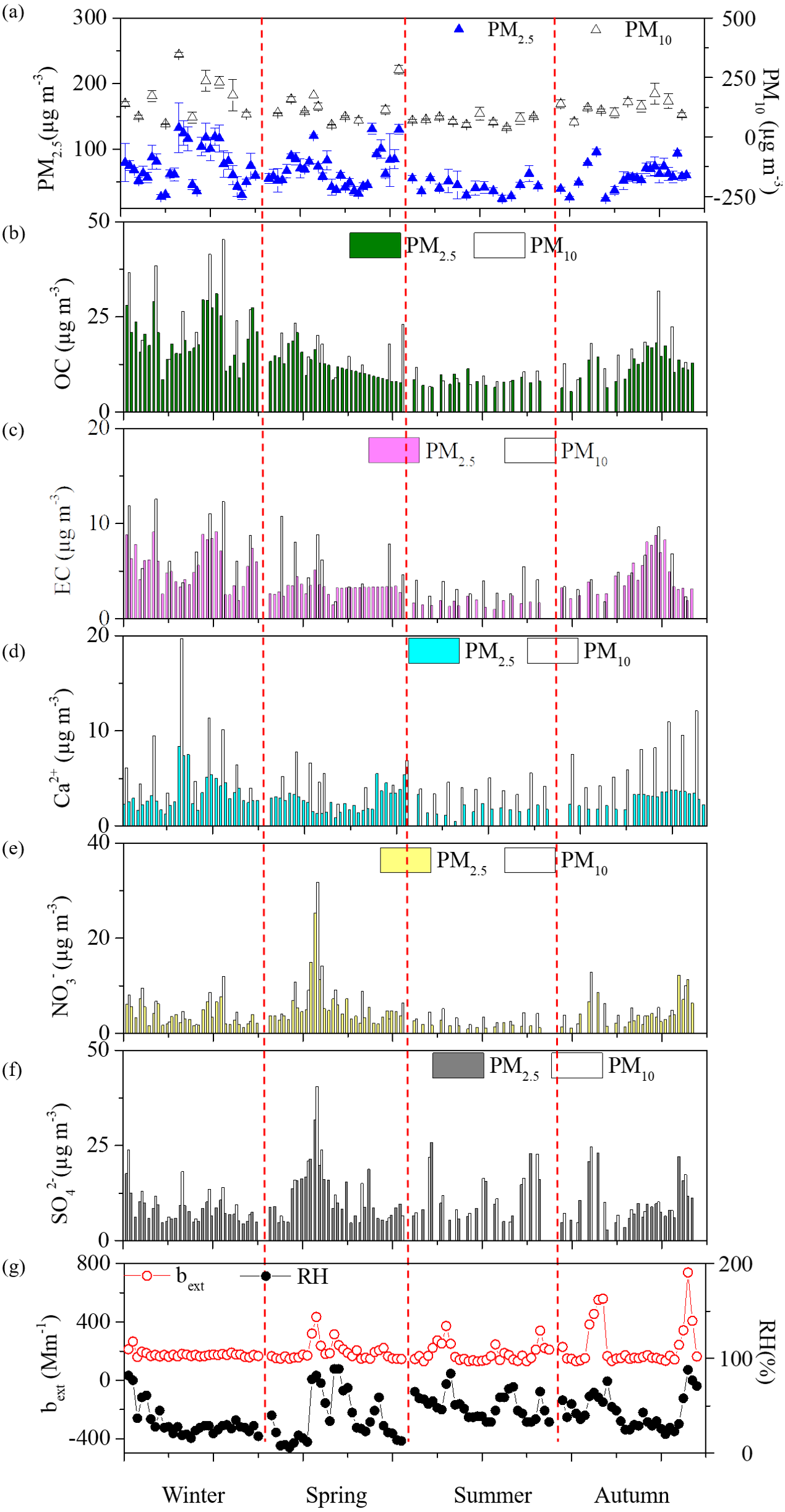
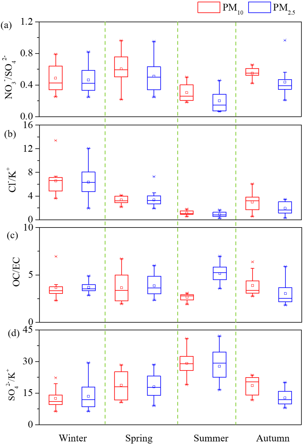
Seasonal variations of PM, OC, EC, three major ions Ca2+, NO3−, and SO42− were shown in Fig. 2. In general, all the species were highest during winter but lowest during summer. During spring, PM10 and PM2.5 mean levels for dust dominated days were 283.4 µg m−3 and 130.4 µg m−3, which were both over 1.7 times of the spring average values. Two dust events were observed in winter and spring, leading the yearly highest PM10 Ca2+ concentrations of 19.7 µg m−3 (winter) and 12.9 µg m−3 (spring). The Ca2+ levels during dust events were over double of seasonal average values for both PM10 and PM2.5 and this phenomenon was consistent with the report of previous literatures (Wang et al., 2013; Shen et al., 2014). Box plot variations of NO3−/SO42−, Cl−/K+, OC/EC, and SO42−/K+ ratios have been also presented (Fig. 3) the average SO42−/K+ ratios were 19.8 for PM10 and 18.0 for PM2.5. High SO42−/K+ ratio indicated important coal combustion contribution to PM. In addition, Cl−/K+ ratios were 3.1.
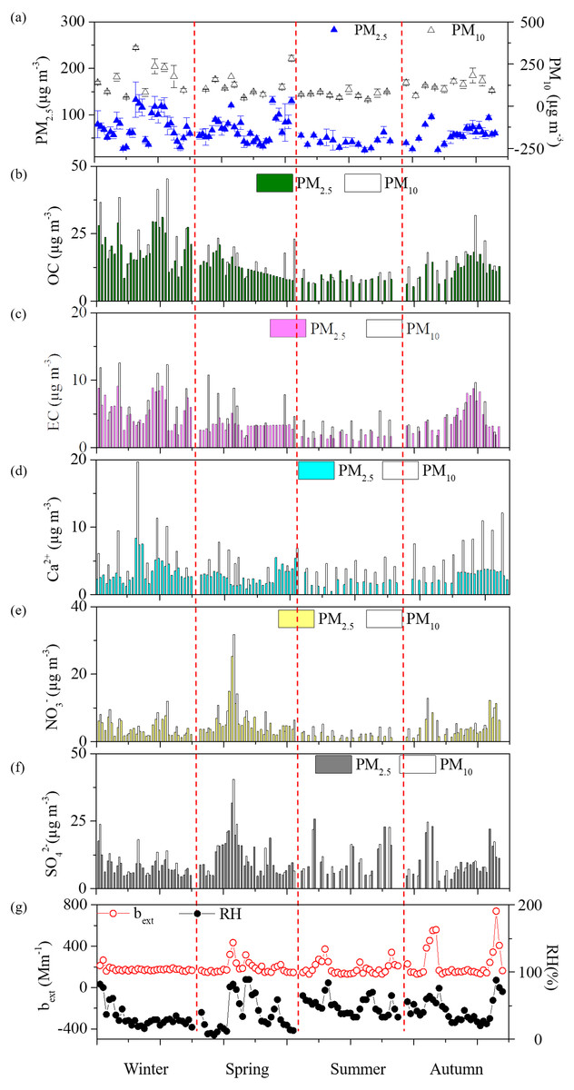
Figure 2: Temporal variations of (A) PM and their chemical components of (B) OC, (C) EC, (D) Ca2+, (E) NO3−, (F) SO42−, and (G) bext and RH at Yulin during four seasons.
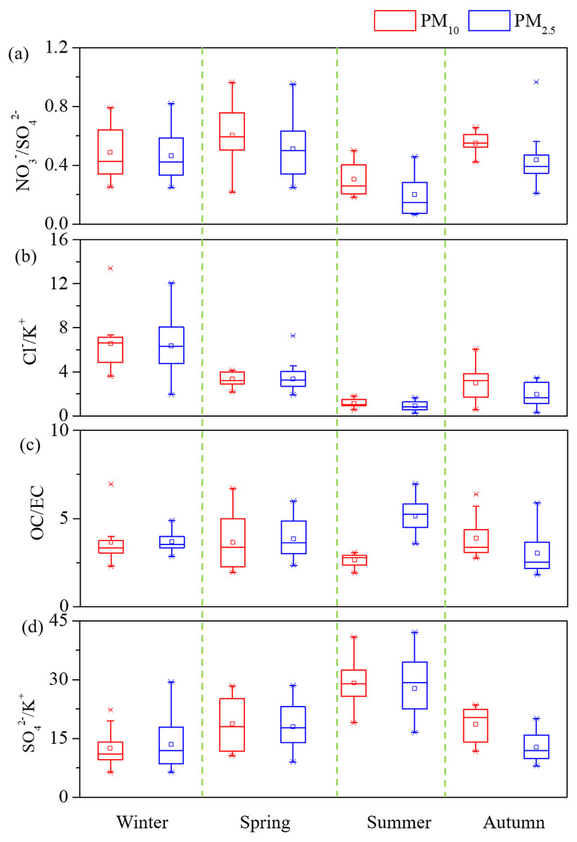
Figure 3: Box plot (10th, 25th, 50th, 75th, and 90th percentile; square pots: mean values) variations of (A) NO3−/SO42−, (B) Cl−∕K+, (C) OC/EC and (D) SO42−/K+ of PM.
The highest PM2.5 OC/EC ratios was observed during summer (5.2), followed by spring (3.9), winter (3.7), and autumn (3.0), which was consistent with the value as Cao et al. (2012a) illustrated. The regressions between OC and EC in PM10 and PM2.5 were plotted as shown, respectively (Fig. S1). Most spots of the PM10 and PM2.5 OC/EC ratios are displayed under the coal combustion line, which indicated important contribution of coal combustion (Cao et al., 2005). Strong correlation coefficients (R) of 0.87 for PM10 and 0.86 for PM2.5 were found between OC and EC. High correlations (Fig. S2) showed cations and anions were the major ions extracted from the PM samples. The seasonal A/C ratios were 0.8, 0.8, 0.6, and 0.7. The major fraction of deficit anions in spring should be carbonate concentration (CO32−) (Shen et al., 2007; Shen et al., 2009). Material balance (Fig. S3) in the following parts revealed that mineral dust was one of major components in aerosol particle mass, and strong PM alkaline should attribute to high dust loading. A triangular diagram was created to show clearly the neutralization contribution of these three cations (Fig. S4). The yearly mean NF values of Ca2+, NH4+, and Mg2+ were 0.25, 0.17, and 0.02. It was clear that Ca2+ and NH4+ were the major neutralizers.
Seasonal variations and source apportionment of light extinction
Daily averaged VR (Table S2) was 21.6 ± 7.3 km. Wind speeds (2.9 m s−1for both spring and summer) and temperature (13 °C for spring and 23 °C for summer) inferred higher mixing and dispersion than those during winter. As shown in Table 2, winter bext (calculated from section 2.3) showed the highest with an average of 232.95 ± 154.88 Mm−1, followed the decrease order of autumn >summer >spring, which were similar in Xi’an (Cao et al., 2012b).
| Chemical species | PM10 | PM2.5 | ||||||
|---|---|---|---|---|---|---|---|---|
| Factor 1 | Factor 2 | Factor 3 | Factor 4 | Factor 1 | Factor 2 | Factor 3 | Factor 4 | |
| Na+ | 0.655 | −0.048 | 0.617 | −0.335 | 0.627 | −0.224 | 0.443 | −0.285 |
| NH4+ | 0.287 | 0.893 | −0.145 | 0.226 | 0.201 | 0.951 | 0.107 | −0.035 |
| K+ | 0.69 | 0.386 | 0.318 | −0.237 | 0.687 | 0.521 | 0.199 | −0.185 |
| Mg2+ | 0.55 | −0.313 | 0.589 | 0.226 | 0.337 | −0.416 | 0.693 | −0.265 |
| Ca2+ | 0.683 | −0.37 | 0.414 | 0.186 | 0.408 | −0.485 | 0.537 | −0.221 |
| F− | 0.752 | −0.024 | −0.115 | −0.384 | 0.665 | −0.35 | −0.118 | −0.169 |
| Cl− | 0.813 | 0.008 | 0.262 | −0.389 | 0.885 | −0.117 | −0.033 | 0.093 |
| NO3− | 0.374 | 0.776 | 0.209 | 0.174 | 0.343 | 0.735 | 0.372 | −0.023 |
| SO42− | 0.923 | 0.849 | 0.274 | 0.194 | 0.896 | 0.893 | 0.229 | −0.096 |
| OC1 | 0.773 | 0.07 | −0.443 | −0.238 | 0.898 | −0.113 | −0.196 | −0.033 |
| OC2 | 0.892 | 0.035 | −0.33 | 0.058 | 0.908 | 0.091 | −0.108 | 0.242 |
| OC3 | 0.886 | −0.123 | −0.165 | 0.12 | 0.932 | −0.058 | −0.132 | 0.153 |
| OC4 | 0.944 | −0.221 | −0.066 | 0.063 | 0.914 | −0.097 | −0.126 | 0.023 |
| EC1 | 0.895 | −0.014 | −0.346 | −0.024 | 0.912 | 0.057 | −0.243 | 0.001 |
| EC2 | 0.716 | −0.114 | −0.14 | 0.329 | 0.707 | −0.212 | 0.081 | 0.366 |
| EC3 | 0.531 | −0.39 | 0.102 | 0.546 | 0.01 | −0.017 | 0.653 | 0.712 |
| OP | 0.916 | −0.003 | −0.276 | 0.029 | 0.828 | 0.225 | −0.314 | −0.099 |
| % Var | 23.9 | 7.6 | 58.1 | 7.3 | 27.8 | 11.3 | 47.1 | 3.6 |
Notes:
- % Var
-
percentage of the variance explained by each factor
According to section 3.1 and mass balance results (Fig.S2), (NH4)2SO4, NH4NO3, OM, EC, the major contributors to PM. Moreover, coarse matter (CM) was important contributor to bext as a result of high PM10 concentrations (Cao et al., 2012a). In this study, unidentified chemical species were summed up and revered as “Others” below. In general, the bext can be estimated statistically as follows: (14)
bext and chemical species mass concentrations are presented with the Mm−1 and µg m−3 unit, respectively. fL(RH) is the growth curves of sulfate and nitrate, which can be found in IMPROVE net results (Pitchford et al., 2007). fL(RH) was used in this study because sulfate and nitrate mass are distributed in droplet mode.
Potential sources and transport pathways of PM2.5
In order to investigate the PM2.5 potential advection, PSCF analysis was conducted in this study (Petit et al., 2017). Figure 4 shows the PCSF analysis results from December 2013 to October 2014, which suggested that local emissions, as well as certain regional transport from northwesterly and southerly areas, contributed to PM2.5 loadings during the whole year. As average PM2.5 values were lower than 75 µg m−3 in summer, some differences were found during the other three seasons. During winter, the potential source area has been recorded; it was mainly from local emissions. Besides, low potential source area was from the northwestern plain areas of Ningxia Hui Autonomous Region and Xinjiang Uyghur Autonomous Region. In contrast to winter, higher potential source regions for PM2.5 during spring stretched to local emissions and the juncture of Guanzhong Plain, Henan province, Inner Mongolia and Ningxia Hui Autonomous Region.

Figure 4: Potential source areas for PM2.5 in Yulin during (A) annual, (B) winter, (C) spring, and (D) autumn.
The color code denotes the PSCF probability. The measurement site is indicated with a red circle.
Source apportionment of PM
In this study, PCA analyses have been conducted to apportion the PM sources. The fundamental principle of PCA is that a strong correlation may exist between components from the same source. It searches factors that play the leading roles by analysis of correlation and variance. Multivariate factor analysis was adopted to help identification of dominant source categories and the results obtained by varimax rotated factor analysis for both PM10 and PM2.5 are presented in Table 3.
| Chemical species | PM10 | PM2.5 | ||||||||
|---|---|---|---|---|---|---|---|---|---|---|
| Factor 1 | Factor 2 | Factor 3 | Factor 4 | Communality | Factor 1 | Factor 2 | Factor 3 | Factor 4 | Communality | |
| Na+ | 0.655 | 0.048 | 0.617 | 0.335 | 0.8234 | 0.627 | 0.224 | 0.443 | 0.285 | 0.8189 |
| NH4+ | 0.287 | 0.893 | 0.145 | 0.226 | 0.8434 | 0.201 | 0.951 | 0.107 | 0.035 | 0.8674 |
| K+ | 0.69 | 0.386 | 0.318 | 0.237 | 0.9123 | 0.687 | 0.521 | 0.199 | 0.185 | 0.9312 |
| Mg2+ | 0.55 | 0.313 | 0.589 | 0.226 | 0.8822 | 0.337 | 0.416 | 0.693 | 0.265 | 0.8659 |
| Ca2+ | 0.683 | −0.37 | 0.414 | 0.186 | 0.8956 | 0.408 | 0.485 | 0.537 | 0.221 | 0.9187 |
| F− | 0.752 | 0.024 | 0.115 | 0.384 | 0.9231 | 0.665 | −0.35 | 0.118 | 0.169 | 0.9052 |
| Cl− | 0.813 | 0.008 | 0.262 | 0.389 | 0.9453 | 0.885 | 0.117 | 0.033 | 0.093 | 0.9312 |
| NO3− | 0.374 | 0.776 | 0.209 | 0.174 | 0.9204 | 0.343 | 0.735 | 0.372 | 0.023 | 0.9124 |
| SO42− | 0.923 | 0.849 | 0.274 | 0.194 | 0.9663 | 0.896 | 0.893 | 0.229 | 0.096 | 0.9645 |
| OC1 | 0.773 | 0.07 | 0.443 | 0.238 | 0.8154 | 0.898 | 0.113 | 0.196 | 0.033 | 0.8069 |
| OC2 | 0.892 | 0.035 | −0.33 | 0.058 | 0.8798 | 0.908 | 0.091 | 0.108 | 0.242 | 0.8123 |
| OC3 | 0.886 | 0.123 | 0.165 | 0.12 | 0.8332 | 0.932 | 0.058 | 0.132 | 0.153 | 0.8397 |
| OC4 | 0.944 | 0.221 | 0.066 | 0.063 | 0.8120 | 0.914 | 0.097 | 0.126 | 0.023 | 0.8189 |
| EC1 | 0.895 | 0.014 | 0.346 | 0.024 | 0.8987 | 0.912 | 0.057 | 0.243 | 0.001 | 0.8759 |
| EC2 | 0.716 | 0.114 | −0.14 | 0.329 | 0.8824 | 0.707 | 0.212 | 0.081 | 0.366 | 0.9325 |
| EC3 | 0.531 | −0.39 | 0.102 | 0.546 | 0.7923 | 0.01 | 0.017 | 0.653 | 0.712 | 0.8261 |
| OP | 0.916 | 0.003 | 0.276 | 0.029 | 0.8090 | 0.828 | 0.225 | 0.314 | 0.099 | 0.8267 |
| % Var | 23.9 | 7.6 | 58.1 | 7.3 | Total 96.9% | 27.8 | 11.3 | 47.1 | 3.6 | Total 89.8% |
| Eigen value | 5.34 | 3.45 | 2.67 | 1.6 | 6.52 | 2.87 | 2.91 | 1.23 | ||
Notes:
- % Var
-
percentage of the variance explained by each factor
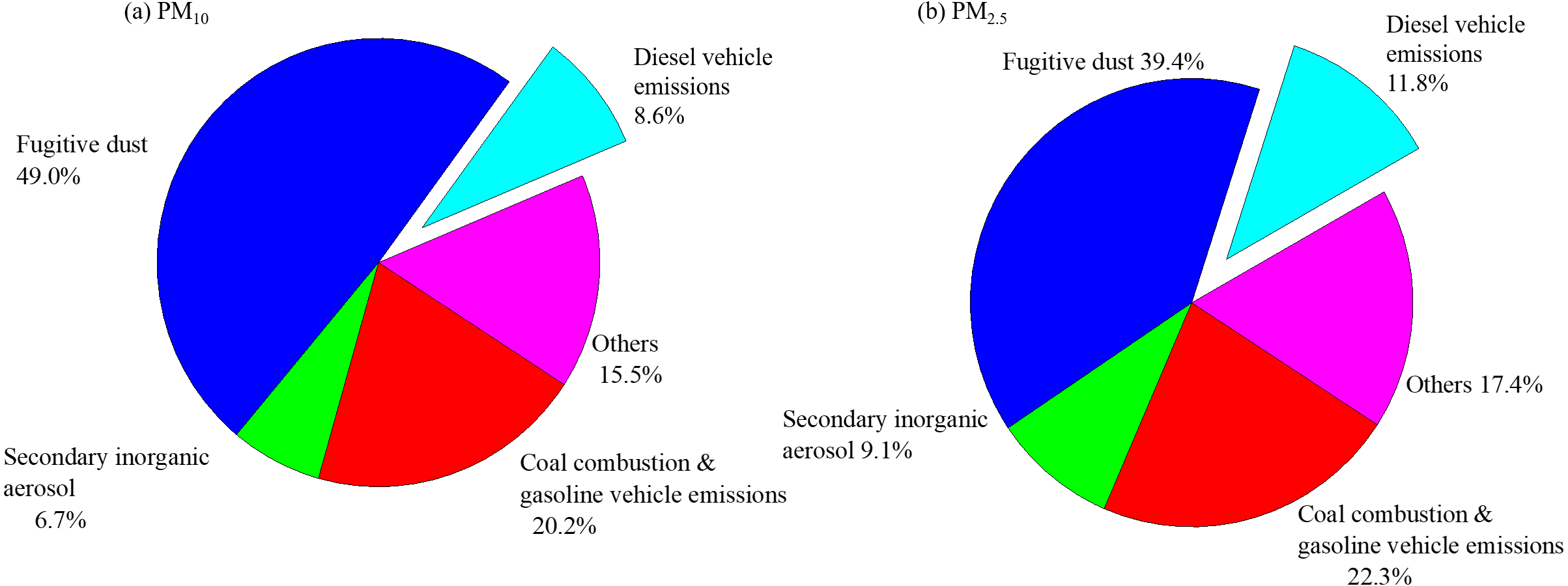
The fugitive dust was the most major source of PM, followed by coal combustion & gasoline vehicle emissions, secondary inorganic aerosol, and diesel vehicle emissions for both PM10 and PM2.5 (Fig. 5). For PM10, Factor 1 was responsible for 23.9% of the total variance and had highly positive contributions from SO42−, Cl−, OC four fractions, EC1, EC2, and OP, indicating its relation to coal combustion and gasoline vehicle emission (Huang et al., 2013). Factor 2 (7.6% of the total variance) had highly correlation with NH4+, SO42−, and NO3−, which represented the source of secondary inorganic aerosols (Shen et al., 2011). The fugitive dust was a main contributor to PM10, with a contribution of 58.1% (Zhang et al., 2014). Factor 4 should be responsible for 7.3% of the total variance and had highly positive contributions from EC3, indicating its relation to diesel vehicle exhaust (Shen et al., 2011). However, PM2.5 showed some differences. Factors 1, 2, 3, and 4 represented the source of, diesel exhaust, coal combustion& gasoline exhaust, secondary inorganic aerosols, fugitive dust and diesel vehicle exhaust, accounting for 27.8%, 11.3%, 47.1% and 3.6% of the total variance, respectively.

Figure 5: Source contribution analyses for (A) PM10 and (B) PM2.5 defined by PCA analyses.
The source apportionments of PM were presented in Fig. 5. PM10 showed a maximum contribution of 49.0% from fugitive dust. The coal combustion& gasoline vehicle emissions contributed 20.2%, while the contribution from secondary inorganic aerosols and diesel vehicle exhaust were found to be 6.7% and 8.6%, respectively. In the case of PM2.5, 39.4% of the mass has been contributed by 39.4% and 22.3% from coal combustion& gasoline vehicle emissions. Secondary inorganic aerosol contributed to 9.1% and 11.8% for diesel vehicle exhaust.
Discussion
On a basis of a record of data analysis, this study has demonstrated that fossil fuel especially coal consumption should lead to the high PM pollutions in Yulin. In fact, in our previous study, lower NO3−/SO42− ratio suggests that stationary emission of coal combustion was the dominant source of PM particle (Lei et al., 2018). Coal burning in power plant and resident heating should be the major source of high sulfate. In addition, Industry emissions such as coke production also contributed to high sulfate. Sulfate, the most abundance component, highlighted coal combustion contribution to PM.
As Yulin is located in the cross border between desert and the Chinese loess, high spring PM levels should attribute to increasing of eolian dust. Prior studies also reported that heavy dust storm events in Yulin led to high TSP levels in spring of 257 µg m−3 (Zhang et al., 2003). In contrast, cities far away from the desert showed a different seasonal pattern compared to Yulin. High Ca2+ levels in winter and autumn should attribute to urban fugitive dust emitted by high wind from road and construction sites. The domestic heating period in Yulin started from November 1 to April 30 the next year. One hand, high SO42− concentrations observed during spring was mainly due to the domestic heat. The average wind speed and RH were 2.86 m s−1 and 38%, which were a little higher than those during summer. However, the temperature during spring was 13 °C, which could enhance the strong gas-particle transfer conversions of SO2 to SO42−. In contrast, high summer sulfate should mainly due to high temperature enhancing the strong gas-particle transfer conversions of SO2 to SO42−, as suggested in some studies (Wang et al., 2012; Shen et al., 2014). Winter lower SO42− levels attribute to high wind speed (2.56 m s−1 in average) favorable to diffusion and low relative humidity (33% in average) unfavorable to sulfate formation. High winter and low spring sulfate were observed in Xi’an, which showed a difference seasonal pattern when compared to Yulin (Shen et al., 2014). High winter sulfate was due to coal combustion in heating season and unfavorable diffusion condition in Xi’an (low wind speed, averaged 1.45 m s−1, and high RH, 55.9% in average). Lower NO3−/SO42− ratio suggests that stationary emissions are a dominant source of PM particles which has also been reported in Lei et al. (2018). Summer NO3−/SO42− ratios were the lowest for both PM10 and PM2.5, which because high temperature can favor SO2 converted to SO42−, while low RH was unfavorable the NO3− formation (Shen et al., 2008). High SO42−/K+ and Cl−/K+ ratios indicated important coal combustion contribution to PM (Shen et al., 2009).
High summer PM2.5 OC/EC ratio inferred a dominant fraction of OC from gas-particle conversion. In fact, high temperature and atmospheric oxidation in summer favored the secondary organic carbon (SOC) formation (Wang et al., 2012). The regressions between OC and EC in PM10 and PM2.5 were plotted as shown, respectively (Fig. S1). Most spots of the PM10 and PM2.5 OC/EC ratios are displayed under the coal combustion line, which indicated important contribution of coal combustion (Cao et al., 2005). High sulfate and OC levels also supported our conclusion. The regression equation intercepts for PM2.5 and PM10, indicated that OC primary non-combustion emissions, such as regional background carbonaceous species, long range transport, and local biological detritus, influenced heavily on fine particles in comparison with coarse fraction (Turpin & Huntzicker, 1995). Seasonal A/C ratios variations showed that spring PM samples were more alkaline because of the high loadings of Ca2+ and Mg2+ (Shen et al., 2014). The neutralization contributions illustrated that low contribution of Mg2+ changed the PM from weakly acidic to weakly alkaline in many PM samples.
Good correlations in different seasons were found between the reconstructed bext and the bext estimated by visibility (Fig. S5). A summary of the light extinction source apportionment results were presented in Table 2. On average, CM, NH4NO3 and(NH4)2SO4 were the most chemical species contributing to bext. (NH4)2SO4 accounted highest in summer (34.39 ± 14.79%), while NH4NO3showed the large contribution in autumn. During winter, (NH4)2SO4 also was the highest during winter followed by CM. These results indicated that the extinction effects from (NH4)2SO4 and NH4NO3 significantly increased under high RH conditions during summer and winter.
PSCF results have shown that dust was the most abundant components during spring, which was due to the atmospheric dust transport. Unlike winter and spring, potential source area was mainly from local emissions and low potential source areas were from northerly areas like Guanzhong Plain. This is consistent with the dominant source from coal combustion related above (Liu et al., 2015). PCA results showed the fugitive dust and coal combustion dominated the PM loadings both in PM10 and PM2.5 over Yulin. Moreover, local emissions and some certain regional transport were the main sources. Despite the dust transportation, the economic boom in Yulin gave rise to substantial air pollution. In order to improve the air quality, strict measurements should be launched in both local and regional areas.
Conclusions
The chemical species for PM were analyzed and their associated sources were identified in Yulin, China. PM levels, OC, EC were highest during winter and lowest during summer. High Ca2+ levels during winter and autumn should attribute to fugitive dust. High spring and summer sulfate levels should be due to different sources. Ion balance illustrated that PM10 samples were more alkaline than PM2.5. Winter bext showed the highest with an average of 232.95 ± 154.88 Mm−1, followed by autumn, summer, and spring. The regression equation intercepts for different values in PM2.5 and PM10 indicated that OC primary non-combustion emissions, such as regional background carbonaceous species, long range transport, and local biological detritus, influenced heavily on fine particles in comparison with coarse fraction. Light extinction source apportionment results inferred that the extinction effects from hygroscopic species, such as, (NH4)2SO4, NH4NO3, increased significantly under high RH conditions during summer and winter. High SO42−/K+ and Cl−/K+ ratio indicated the important contribution of coal combustion. PCA analyses results showed that the fugitive dust was the most major source of PM, followed by coal combustion & gasoline vehicle emissions, secondary inorganic aerosol and diesel vehicle emissions. PSCF results suggested that PM2.5 were mainly from both local emissions and regional transport from northwesterly and southerly areas during the whole year.