
Century-scale changes in phytoplankton phenology in the Gulf of Maine
- Published
- Accepted
- Received
- Academic Editor
- Hugo Sarmento
- Subject Areas
- Climate Change Biology, Biological Oceanography
- Keywords
- Phenology, Climate, Phytoplankton, Chlorophyll, Bloom, Gulf of Maine
- Copyright
- © 2019 Record et al.
- Licence
- This is an open access article distributed under the terms of the Creative Commons Attribution License, which permits unrestricted use, distribution, reproduction and adaptation in any medium and for any purpose provided that it is properly attributed. For attribution, the original author(s), title, publication source (PeerJ) and either DOI or URL of the article must be cited.
- Cite this article
- 2019. Century-scale changes in phytoplankton phenology in the Gulf of Maine. PeerJ 7:e6735 https://doi.org/10.7717/peerj.6735
Abstract
The phenology of major seasonal events is an important indicator of climate. We analyzed multiple datasets of in situ chlorophyll measurements from the Gulf of Maine dating back to the early 20th century in order to detect climate-scale changes in phenology. The seasonal cycle was consistently characterized by a two-bloom pattern, with spring and autumn blooms. The timing of both spring and autumn blooms has shifted later in the year at rates ranging from ∼1 to 9 days per decade since 1960, depending on the phenology metric, and trends only emerged at time scales of >40 years. Bloom phenology had only weak correlations with major climate indices. There were stronger associations between bloom timing and physical and chemical variables. Autumn bloom initiation correlated strongly with surface temperature and salinity, and spring bloom with nutrients. A later spring bloom also correlated with an increased cohort of Calanus finmarchicus, suggesting broader ecosystem implications of phytoplankton phenology.
Introduction
One of the earliest studied and most striking oceanographic phenomena is the spring phytoplankton bloom. A prominent feature of satellite images, the bloom initiates as “flowerings of diatoms, resulting in local swarms so dense as to be the most spectacular event in the yearly planktonic cycle” (Bigelow, 1924a). Efforts to predict the timing of the spring bloom in the Gulf of Maine helped to coalesce the interdisciplinary and quantitative approaches that underlie modern oceanography (Riley, 1949). Despite over 100 years of study and a corpus of theory, predicting the dynamics of phytoplankton blooms remains an important but elusive goal (Sverdrup, 1953; Taylor & Ferrari, 2011; Mahadevan et al., 2012; Behrenfeld & Boss, 2014; Zarubin, Lindemann & Genin, 2017).
Phytoplankton blooms are indeed spectacular events, and their timing is particularly important to marine ecosystems in strongly seasonal climes. Because they constitute the primary source of carbon fixation for the pelagic food web, animals across trophic levels have life history strategies tuned to the seasonal cycle of production. Productive systems depend on seasonal timing matches between trophic levels because mismatches in timing can mean that a grazer or predator misses its feeding window (i.e., match-mismatch hypothesis, (Cushing, 1969; Edwards & Richardson, 2004). The Gulf of Maine is a quintessential example of this phenomenon. The zooplankton community is largely copepods of the genus Calanus (Bigelow, 1924a), which time their emergence from diapause to exploit the spring phytoplankton bloom. The pulse of Calanus production is then succeeded by fish (Golet et al., 2015), mammal (Pershing et al., 2009), and other migrations.
There is growing attention to changing phenology as both an indicator and a consequence of climate change. Understanding phenology in a climate context requires time series that span many decades. Such datasets in the pelagic ocean are limited. In the Gulf of Maine, there have been noted phenological shifts in recent times, particularly regarding physical properties such as temperature (Thomas et al., 2017), stratification, and hydrology (Smith et al., 2012), related to climate change. To understand the associated phenological changes in the pelagic ecosystem in a climate context, we need biological time series that span many decades—in seasonal oceans a minimum of 40 years (Henson et al., 2010). To examine changes in phytoplankton phenology in the Gulf of Maine at the climate scale, we aggregated multiple datasets of in situ chlorophyll measurements over the past century. We used these data to address the following questions: (1) Has the timing of phytoplankton blooms changed over the past century? (2) What are the drivers of these changes? And (3) What are the ecological consequences of these changes?
Data and Methods
Phytoplankton dataset
We aggregated datasets of in situ phytoplankton measurements from multiple public sources. We used chlorophyll (generally chlorophyll-a) as an estimate of phytoplankton biomass and used previously published datasets. Chlorophyll time series in the interior Gulf of Maine vary together based on empirical orthogonal function analysis, separately from the coastal Gulf of Maine (Thomas, Townsend & Weatherbee, 2003). This analysis thus focused on the inner Gulf of Maine, including all samples deeper than the 100 m isobath (106,257 samples, Fig. 1). For some data, measurements were in standard units (mg chl m−3). For others, a conversion was necessary. For phytoplankton colour index (PCI) measured by the continuous plankton recorder (CPR) and for Forel-Ule (FU) scale, we used established relationships for conversions, which for PCI was categorical (Raitsos et al., 2005) and for FU was exponential (Wernand, Van der Woerd & Gieskes, 2013). These conversion relationships are from global datasets, contain uncertainty, and possibly unknown variability in space and time. The fact that our analysis focuses on the timing of events and is less reliant strictly on magnitude should minimize potential biases. The data were all from calibrated, quality-controlled, public databases: Aggregated database of (Boyce, Lewis & Worm, 2012, 1934–2010, mg chl m−3 and FU), Continuous Plankton Recorder (1961–2013, PCI), Gulf of Maine North Atlantic Time Series (1998–2015, mg chl m−3 and FU (Balch et al., 2016), including measurements from (Bigelow, 1924b), and the World Ocean Database (Boyer et al., 2013) (1934–2010, mg chl m−3 and FU). In the post-1960 period, most datasets were largely gap-free during the indicated sampling years, with the exception of FU measurements, which were sporadic throughout the time series (<1% of measurements). We averaged these data into a monthly time series, removing duplicates, spanning the time period 1912–2015.
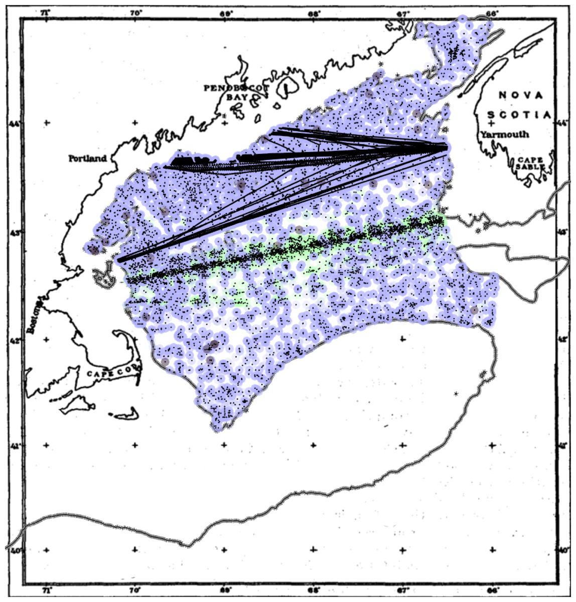
Figure 1: Sample locations for the compiled phytoplankton dataset in the inner Gulf of Maine.
Points are back-colored by original measurement type: FU (grey), PCI (green), chlorophyll (blue). Background map adapted from (Bigelow, 1924a). The grey line is updated 100 m isobath.
We tested the accuracy and limitations of a temporal cubic spline interpolation for missing data. We validated the interpolation by removing each data point, interpolating, comparing the interpolated value to the measured value, and comparing the phenology metric (described below) calculated from the interpolation to that calculated from the measured value. For an interpolation that only included points not surrounded by missing data, the interpolated values compared well to measured values (r = 0.37, p ≪ 0.0001 over all points, and r > 0.99, p ≪ 0.0001 for phenology metrics). When the interpolation was tested for points surrounded by missing data, there was no significant correlation between interpolated and measured values, so we did not interpolate beyond one point.
Oceanographic datasets
We assembled oceanographic time series to compare to chlorophyll phenology. We used previously published data for water column physics (Fisheries and Oceans Canada, climate database, http://www.bio.gc.ca/science/data-donnees/base/run-courir-en.php, (Gregory, 2004) and nutrients (Rebuck & Townsend, 2014). We used measurements that fell within the spatial domain matching the chlorophyll dataset and averaged to monthly values. Physical data included temperature (T) and salinity (S) averaged over the upper 50 m. We also included a stratification index (Δ), estimated as the difference of mean density (σT) between the surface (0–50 m) and deep (50 m - bottom) layers (Drinkwater & Gilbert, 2004). Chemical data included surface NO3+NO2, Si(OH)4, and PO4 measurements, using only those measurements that passed all quality control criteria (Rebuck & Townsend, 2014). We also used annual climate indices: the Atlantic Multidecadal Oscillation (AMO), North Atlantic Oscillation (NAO), Gulf Stream Index (GSI), the Arctic Ocean Oscillation (AOO), and the Arctic Oscillation (AO) (cf NOAA Climate Prediction Center).
Grazer dataset
We used copepod count data from the CPR. The dominant seasonal copepod in the central Gulf of Maine is Calanus finmarchicus (Runge et al., 2014), which has a seasonal peak in surface waters following the spring bloom. Adults emerge from diapause and exploit the spring bloom for egg production. This cohort reaches adulthood in the late spring and summer. We calculated a mean log anomaly for late-stage (copepodite 5–6) C. finmarchicus for May–July, as an index of how well this species fares following the spring bloom. We did not compute an analogous autumn time series because C. finmarchicus has entered diapause at depth by that time, and the CPR makes surface measurements.
Analysis
We used a clustering analysis to examine the shape(s) of the bloom cycle across years. This helped to confirm that our phenology metrics were applicable, and also to detect changes in the bloom pattern across time. We clustered years based on the shape of the seasonal cycle of chlorophyll following the methodology of Foukal & Thomas (2014): briefly, we used k-means multivariate clustering, with the squared Euclidean distance as the similarity metric and randomly selected starting centroids. Other similarity metrics yielded qualitatively similar results. To account for the randomness in the algorithm, we computed an ensemble of 100 runs, sorted clusters by frequency, and analyzed the modal clusters for each year.
We produced time series of phenology metrics for spring and autumn blooms. There are many metrics for quantifying the timing of phytoplankton blooms, with most metrics targeting the timing of either bloom initiation or bloom peak (Ji et al., 2010; Brody, Lozier & Dunne, 2013). Bloom shape can vary from year to year and by location, so no single metric has emerged as the preferred choice. Because of the coarse temporal resolution (1 month), some phenology metrics were not appropriate for this dataset. We computed five phenology metrics for the spring and autumn blooms:
-
μm - Timing of maximum. Because the dataset is binned monthly, this is a coarse time series; values are midpoints of months.
-
μc - Center of mass. This metric computes the center of mass within the February-May time period (spring index) and of the August-November time period (autumn index), and provides a smooth metric.
-
μg - Midpoint of Gaussian fit. This metric fits a Gaussian curve to half of the year (for spring and autumn indices) and uses the fitted mean (µ) parameter as the bloom peak timing, providing a smooth metric.
-
τd - Timing of maximum increase. This is a coarse (monthly) index of the timing of bloom initiation.
-
τt - Threshold timing. This metric computes the timing at which the total value crosses a threshold that is some percentage of the year’s total (i.e., the cumulative sum method). We computed this metric for multiple thresholds for both spring and autumn indices.
We used the phenology metrics in time series analysis. We examined the time series for statistically significant trends. We then looked for long-term associations with physical drivers and with upper trophic levels to determine the potential causes and consequences of changing phenology. Analysis was performed using Pearson correlation and coherence analysis. The coarse spatio-temporal resolution of the dataset means that there is additional variance around time series and associated relationships, and correlation coefficients reflect that. We took steps to avoid over-reliance on single p-value determinations and dichotomous thinking (McShane & Gal, 2017). While we did use p < 0.05 as one benchmark, we disregarded those correlations driven by an outlier. Furthermore, only correlations that held up for multiple phenology metrics or with very strong relationships were considered robust. For the analysis with the climate indices and the C. finmarchicus time series, the time series were sufficiently long and gap-free to conduct a coherence analysis. We used the minimum variance distortionless response approach (Benesty, Chen & Huang, 2005). We also tested the climate indices at lags of 0–3 years, and for the C. finmarchicus time series, because of the ontogenetic lag and east-to-west hydrographic flow, we compared it to the phenology time series calculated for just the eastern Gulf of Maine (east of >68∘W).
Results
Clustering
Excluding singletons, there were three main bloom types that emerged consistently over the ensemble of cluster calculations (Fig. 2). The most common was the conventional cycle, with a pronounced spring bloom peaking in April, a smaller autumn bloom peaking in October, and a seasonal minimum in January. This cycle type dominated in most of the 1980s and 1990s. The second most common was a two-bloom cycle where the spring and autumn blooms were of closer magnitude to each other, again peaking in April and October. The third cycle type had a pronounced but delayed spring bloom, peaking in May, a diminished autumn bloom, and a higher winter minimum. The second and third cycle patterns appeared sporadically over the later part of the time series. All of these cycle patterns had a predominantly two-peak shape, conducive to the phenology metrics used.
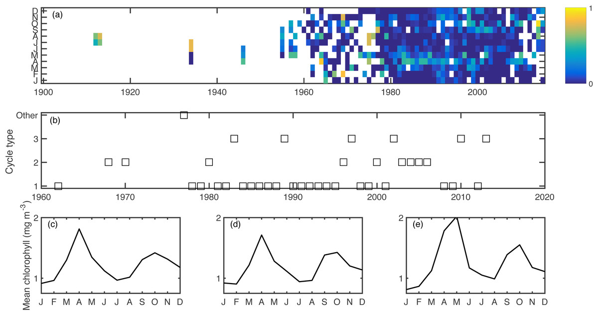
Figure 2: Aggregated chlorophyll dataset (A), showing monthly binned chlorophyll (log mg m−3), including a 1-unit spline interpolation.
Years clustered by cycle type, as computed in the k-means clustering algorithm. (B) Cycle type for each year for which there are sufficient data, showing the most common three cycle types. Seasonal shapes for cycle types 1–3 (C–E) respectively, calculated as the climatology over all years within each cluster.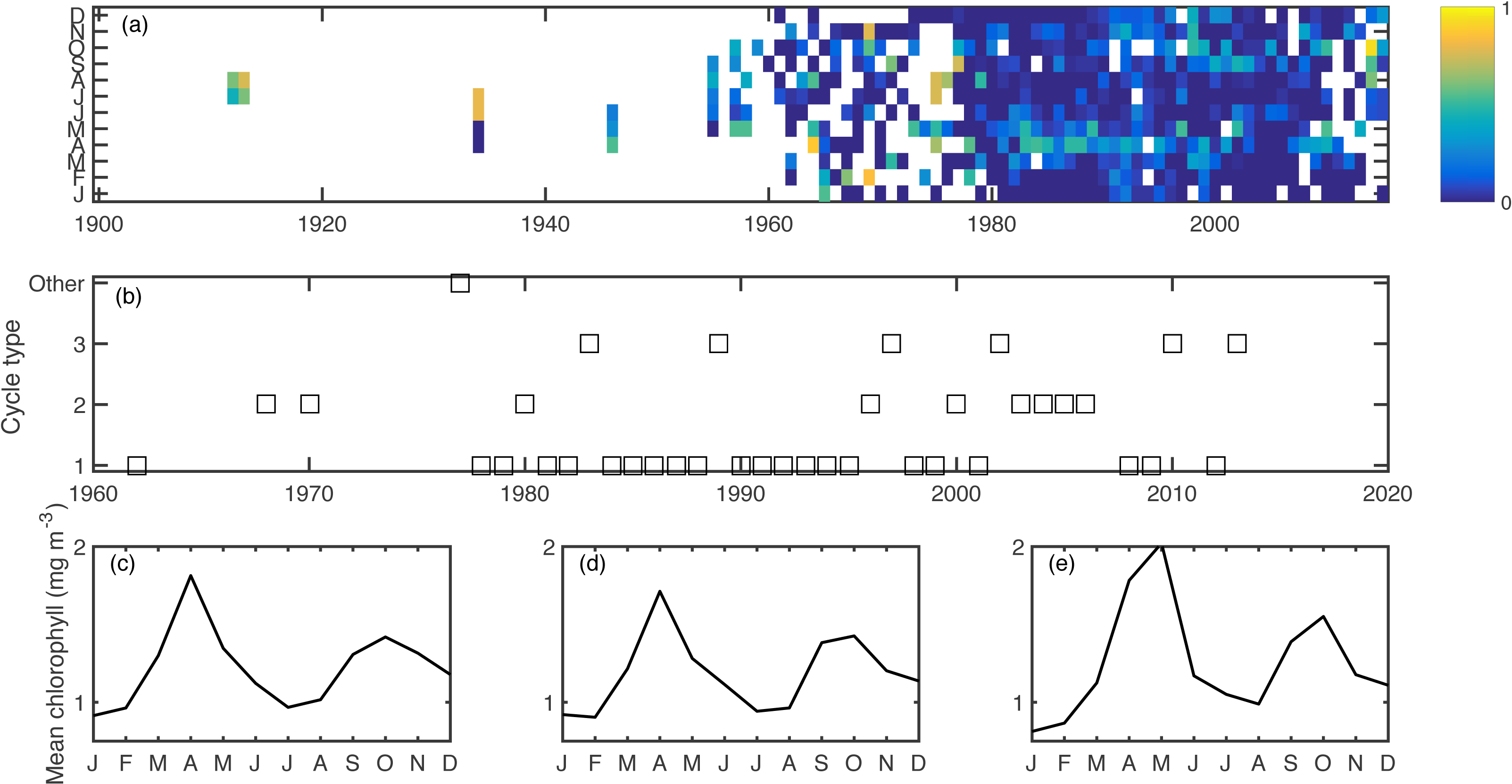
Trends
For all phenology metrics, spring and autumn, the trend over the time series was positive–i.e., shifting later in the year. The strongest trend was for μg, shifting later with mean rates of 8.9 (p = 0.001) and 4.3 (p = 0.02) days per decade (spring and autumn, respectively). Other metrics with noteworthy trends were spring μm (4.4 days per decade, p = 0.1), spring μc (1.5 days per decade, p = 0.1), autumn μc (1.2 days per decade, p = 0.07), and spring τt (4.1 days per decade, p = 0.09). Taking the average of metrics, trends were significant for both spring (p = 0.03) and autumn (p = 0.01), with rates of 3.7 and 3.8 days per decade, respectively. Over the past sixty-year period, where there are enough data to consistently capture the phenology metrics, these shifts equate to a roughly 10–50 day shift in timing. There is substantial inter-annual variance around these trends (Fig. 3A). To test the robustness of these trends to sampling biases, we subdivided the Gulf of Maine into east, west, and coastal sections, divided at 68.5 °W and tested the same phenology metrics for trends. Of the 30 significance tests, 10 were significant at the 0.05 level, 5 were significant at the 0.01 level, and all significant trends were positive for both spring and autumn metrics. We also tested for trends over smaller sliding windows and found that time series of at least 40 years were necessary for significant trends to emerge. Oceanographic variables had statistically significant trends as well, including increases in temperature and stratification and decreases in nitrate+nitrite and phosphate through much of the year (Fig. 3B).

Figure 3: (A) Time series of spring and autumn μg and least squares line showing statistically significant increase since 1960. Shaded area shows the range of all phenology metrics. (B) Significant secular trends for the measured physical and chemical variables during different months and seasons.
Color scale is the strength of the trend as measured by a correlation coefficient (r). Numbers are p values rounded up to the nearest hundredth. Trends with p < 0.05 are colored.
Associations
Correlations between phenology metrics and climate indices were generally weak, with only a few correlations at p < 0.05. Spring and autumn τt correlated positively with the AMO, and autumn τt correlated negatively with the NAO (r2 = 0.17, 0.16, 0.17, respectively). These AMO correlations were also significant at lags of up to three years, with correlations peaking for spring τt at a three year lag (r2 = 0.19), and for autumn τt at a two year lag (r2 = 0.24). Coherence analysis (File S2) also showed weak associations, with r2 typically below 0.2. The notable exceptions were spring phenology metrics and the AO, at ∼3 year periods, and various metrics and the NAO, at both short and long periods, where r2 increases to 0.3–0.4.
Correlations between phenology metrics and ocean physics and chemistry showed a moderate signal with some consistent patterns (Table 1). For spring metrics, the strongest signal was a correlation between stratification and earlier bloom timing. Additionally, high February nutrients correlated with a later bloom, and high June nutrients correlated with an earlier bloom. For autumn metrics there was a consistent pattern across all months of high temperature and salinity correlating with earlier bloom initiation. There was a very strong correlation between October silicate and earlier bloom timing, but these correlations consisted of only four data points.
| SPRING METRICS | |||||
|---|---|---|---|---|---|
| J | F | M | A | M | J |
| Physical variables | |||||
| Δ, τt(−0.93, < 0.01) | T, μg(−0.41, 0.03) | ||||
| Chemical variables | |||||
| N, μm(0.61, 0.05) | N, μg(−0.53, 0.04) | ||||
| N, μc(0.66, 0.03) | Si, μg(−0.55, 0.03) | ||||
| AUTUMN METRICS | |||||
| J | A | S | O | N | D |
| Physical variables | |||||
| T, τd(−0.61, 0.02) | T, τd(−0.68, < 0.01) | T, τd(−0.49, < 0.01) | T, τd(−0.40, < 0.01) | T, τd(−0.50, < 0.01) | S, τt(−0.84, 0.03) |
| T, τt, (−0.55, 0.01) | S, τd(−0.66, < 0.01) | S, τd(−0.71, 0.03) | S, τd(−0.64, 0.05) | S, τd(−0.70, 0.01) | S, τd(−0.64, 0.01) |
| Δ, τd(−0.48, < 0.01) | S, μg(−0.45, 0.02) | ||||
| Δ, τt(−0.55, 0.03) | |||||
| Chemical variables | |||||
| N, μg(−0.51, 0.04) | Si, μg(−0.98, 0.04) | ||||
| Si, μm(−0.96, 0.02) | |||||
| Si, τd(−1.00, < 0.01) | |||||
Grazer analysis
The C. finmarchicus index correlated significantly with μg (r2 = 0.17, p = 0 .01). The western Gulf of Maine C. finmarchicus population is supplied by coastal waters, so we compared the phenology metrics to the C. finmarchicus in the eastern Gulf of Maine (> − 68∘) and found stronger and more consistent correlations: μm (r2 = 0.17, p = 0 .01), μc (r2 = 0.24, p = 0 .003), μg (r2 = 0.26, p = 0 .001). Coherence analysis (Fig. 4) showed that these correlations were largely driven by the long-term secular trend. There was a dip in coherence for periods of approximately 10–40 years. There was also an increase in coherence for periods of <10 years to r2 ≈ 0.2, depending on the metric.
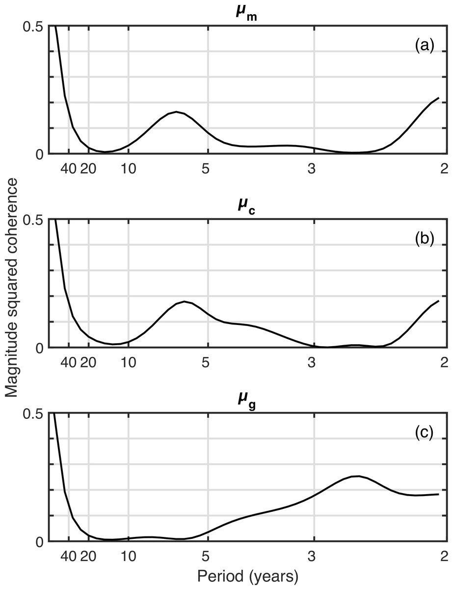
Figure 4: Coherence analysis of three spring phenology metric time series against the time series of late-stage C. finmarchicus abundance.
Discussion
This extended time series of in situ chlorophyll measurements in the Gulf of Maine gives a climate-scale perspective on changing phenology that is not available in the comparatively recent satellite records. Climate-scale changes in the timings of blooms are clear, as are associations between bloom phenology and changing physical conditions as well as changing C. finmarchicus abundance. The most surprising result is that spring bloom timing, primarily using measures of the bloom center, have gotten later at a rate of ∼1–9 days per decade. This shift is apparent when comparing the recent seasonal cycle to that of a few decades ago (Fig. 5). Typically, as the climate warms, summer lengthens, shifting spring events earlier and autumn events later. The shift toward later autumn blooms is consistent with this expectation, but the shift toward later spring blooms is unexpected in this context. Climate indices have been cited to explain recent temperature and ecosystem changes in the Gulf of Maine (Pershing et al., 2015). However, our analysis did not reveal any compelling relationship with the NAO, AMO, GSI, AOO, or AO–the climate oscillations known to be important in the Gulf of Maine—either via direct correlation, lagged correlation, or coherence analysis.
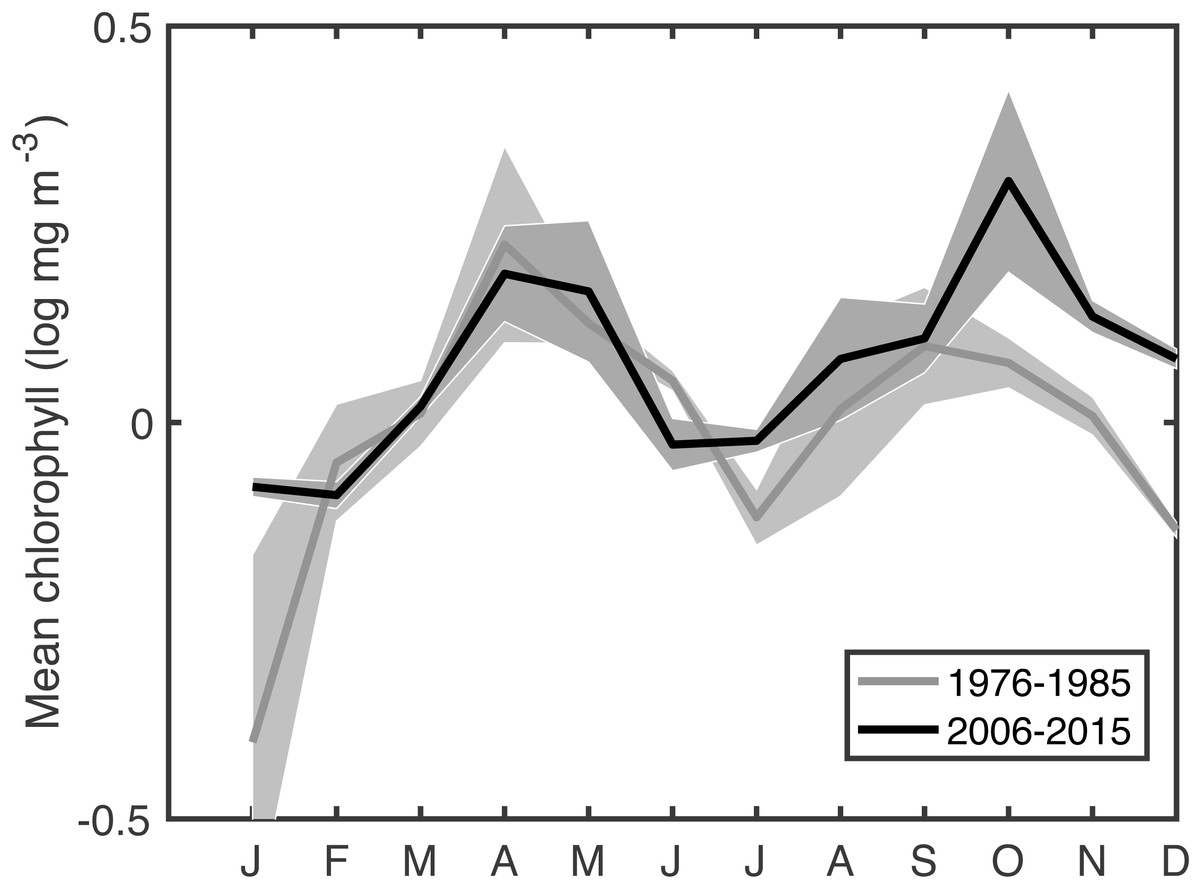
Figure 5: Comparison of mean seasonal cycle of chlorophyll between the most recent decade and an earlier period.
Shaded area shows the variance.
Relationships between bloom phenology and water properties were somewhat more promising. A later spring bloom was associated with lower stratification, higher nutrients near the beginning of the bloom, and lower nutrients near the end of the bloom. Causality is difficult to assign regarding nutrients. Because an earlier spring bloom correlates with decreased February nutrients, and a later spring bloom with decreased June nutrients, it is likely that the bloom is driving the nutrient dynamics through drawdown (or lack thereof), rather than the reverse. The autumn bloom was more tightly associated with changes in physics. Low temperature and salinity are both associated with increased transport of Arctic-origin water via the Labrador Current, which altered autumn bloom patterns during the 1990s (MERCINA Working Group, 2012). The pattern seen here suggests similar physical forcing might have a more consistent long-term effect specifically on the timing of autumn bloom initiation.
It is worth noting the secular trends in conditions, as well as correlations, focus on high-frequency variability and can overlook climate-scale changes. Spring conditions have shifted towards higher stratification and lower nutrients. The timing shift of the spring bloom is consistent with short-term shifts in the three Gulf of Maine zones described by (Ji et al., 2007); they hypothesize that higher stratification causes earlier blooms upstream on the Scotian Shelf, leading to depleted nutrients and later blooms by the time the water mass reaches the central Gulf of Maine. This hypothesis is consistent with our long-term observations and may provide a better explanation for the shift toward later spring blooms.
The positive association between spring bloom timing and late spring C. finmarchicus abundance is notable. If later timing of the center of the bloom is an indication of an extended bloom, then C. finmarchicus emerging from diapause could have a longer window for reproduction, and the first generation cohort would be more abundant than in a typical year. This offers one possible explanation for why the species has persisted in the western Gulf of Maine despite rapid warming and temperatures that should be detrimental to the population (Runge et al., 2014), but would require a consistent upstream supply of late-stage individuals. This shift also runs counter to the expectation of a phenology “mismatch” as conditions change (Edwards & Richardson, 2004).
While this chlorophyll data set gives us new insights into climate-scale phenology changes, there are some caveats to bear in mind. First, chlorophyll is a proxy for phytoplankton. When the oceanography changes, adaptation or replacement of species can occur, and chlorophyll measurements might not capture this. As a means for detecting the major phenological events (i.e., blooms), chlorophyll is probably effective, but this caveat should be kept in mind. Second, the dataset includes measurements that use different methodologies. Measuring chlorophyll “is endlessly complicated by diverse methods of collection and analysis, each with its own virtues but only imperfectly comparable with other methods” (Riley, 1949). Again, the fact that we use relative changes to compute phenology metrics should hedge this caveat, but it should be considered as the data are used in the future.
Conclusion
The shift of both spring and autumn bloom timing toward later dates is surprising. The high range in rate estimates is indicative of the difficulty of quantifying bloom phenology, so the emphasis should be on the consistent directionality across metrics rather than any specific rate. Finally, while the analysis here is suggestive of possible drivers of the shift in bloom timing, a mechanistic explanation for bloom initiation has been an elusive goal in oceanography. As Evans & Parslow (1985) wrote: “Although it seems intuitively reasonable that a sudden effect should have a sudden cause, ecological systems need not behave intuitively. ...[S]pring blooms can occur without any sudden changes in driving variables.” The Gulf of Maine, with its unprecedented rapid changes (Pershing et al., 2015) is often seen as a potential bellwether for other marine systems. The apparent climate-scale shift toward later spring blooms underscores the point that ecosystems do not always change as expected.