
Including autapomorphies is important for paleontological tip-dating with clocklike data, but not with non-clock data
- Published
- Accepted
- Received
- Academic Editor
- Laura Wilson
- Subject Areas
- Computational Biology, Evolutionary Studies, Paleontology
- Keywords
- Total-evidence dating, Parsimony, Tip-dating, Eureptilia, Autapomorphies, BEASTmasteR, Bayesian phylogenetics, Phylogenetic dating, Ascertainment bias, Morphological clock
- Copyright
- © 2018 Matzke and Irmis
- Licence
- This is an open access article distributed under the terms of the Creative Commons Attribution License, which permits unrestricted use, distribution, reproduction and adaptation in any medium and for any purpose provided that it is properly attributed. For attribution, the original author(s), title, publication source (PeerJ) and either DOI or URL of the article must be cited.
- Cite this article
- 2018. Including autapomorphies is important for paleontological tip-dating with clocklike data, but not with non-clock data. PeerJ 6:e4553 https://doi.org/10.7717/peerj.4553
Abstract
Tip-dating, where fossils are included as dated terminal taxa in Bayesian dating inference, is an increasingly popular method. Data for these studies often come from morphological character matrices originally developed for non-dated, and usually parsimony, analyses. In parsimony, only shared derived characters (synapomorphies) provide grouping information, so many character matrices have an ascertainment bias: they omit autapomorphies (unique derived character states), which are considered uninformative. There has been no study of the effect of this ascertainment bias in tip-dating, but autapomorphies can be informative in model-based inference. We expected that excluding autapomorphies would shorten the morphological branchlengths of terminal branches, and thus bias downwards the time branchlengths inferred in tip-dating. We tested for this effect using a matrix for Carboniferous-Permian eureptiles where all autapomorphies had been deliberately coded. Surprisingly, date estimates are virtually unchanged when autapomorphies are excluded, although we find large changes in morphological rate estimates and small effects on topological and dating confidence. We hypothesized that the puzzling lack of effect on dating was caused by the non-clock nature of the eureptile data. We confirm this explanation by simulating strict clock and non-clock datasets, showing that autapomorphy exclusion biases dating only for the clocklike case. A theoretical solution to ascertainment bias is computing the ascertainment bias correction (Mkparsinf), but we explore this correction in detail, and show that it is computationally impractical for typical datasets with many character states and taxa. Therefore we recommend that palaeontologists collect autapomorphies whenever possible when assembling character matrices.
Introduction
In parsimony phylogenetic analyses, the only data informative for reconstructing the tree topology are those with grouping information: potentially shared, derived character states (synapomorphies; Hennig, Davis & Zangerl, 1999). An autapomorphy—a state unique to one terminal taxon or Operational Taxonomic Unit (OTU; Mishler, 2005)—contributes one step to any possible topology. Therefore, autapomorphies are routinely excluded from further analysis in cladistics programs (e.g., the TNT xinact and info commands (Goloboff, Farris & Nixon, 2008); the PAUP* exclude command (Swofford, 2003); and see Yeates, 1992), and autapomorphic characters are often not even collected during assembly of a character-taxon matrix.
In model-based inference, autapomorphies can be informative (Lewis, 2001; Wright & Hillis, 2014), because autapomorphies contribute information about the overall rate of change in the character matrix and site-specific rate heterogenetity. An insufficiently recognized point is that autapomorphies might be particularly important in “tip-dating” analyses, where terminal taxa include fossils with ages older than the present day (Alexandrou et al., 2013; Pyron, 2011; Ronquist et al., 2012; Wood et al., 2013). Tip-dating analyses might be expected to be particularly sensitive to autapomorphies: all autapomorphies occur on terminal branches by definition, so their exclusion will shorten the morphological branchlengths of terminal branches (and thus presumably their time branchlengths), and perhaps increase estimated branch-wise rate variation.
An alternative to inclusion of autapomorphies is ascertainment-bias correction, where the likelihood of unobservable character patterns, Lunobs, is calculated, and the likelihood of the observed data is normalized by dividing by 1 − Lunobs (Felsenstein, 1992; Lewis, 2001). The two common corrections are the Markov-k model with an ascertainment bias correction for the unobservability of invariant characters (Mk-variable-only, or Mkv; Lewis, 2001), and Markov-k with an ascertainment bias correction for parsimony-uninformative characters, Mkparsinf (Allman, Holder & Rhodes, 2010; Ronquist & Huelsenbeck, 2003). These corrections are options in Mr Bayes and can be implemented in Beast1/Beast2 XML, but several studies briefly mention that the scalability and correctness of Mkparsinf computations may be problematic (Dos Reis, Donoghue & Yang, 2016; Koch & Holder, 2012; Matzke, 2016).
The effect of inclusion/exclusion of autapomorphies and ascertainment-bias correction has not been studied in a tip-dating context. Datasets appropriate for doing so are rare because they need to systematically collect all autapomorphies, as well as dates for the OTUs. Müller & Reisz (2006) constructed an all-fossil, morphological matrix of early eureptiles and tested the effect of inclusion/exclusion of autapomorphies in undated Bayesian inference, and recommended including autapomorphies. Lee & Palci (2015) discussed the importance of autapomorphies for tip-dating, but did not test the effect of their inclusion/exclusion. We obtained dates for Müller and Reisz’s taxa, and used the dataset to test the effects of autapomorphy inclusion. Surprisingly, no effect on dates was found. This might be due to the non-clocklike nature of the dataset, an explanation we confirm with a simulation study that shows autapomorphy exclusion biases terminal branchlength estimates when the data are highly clocklike, but not in a non-clock dataset. We also examine the Mkparsinf correction and show that it scales poorly for characters with more than two states, limiting its usability.
Methods
Data
The morphological matrix was taken from Müller & Reisz (2006). The date ranges for OTUs were derived from the literature, following best practices guidelines (Parham et al., 2012). Correlation between time and morphological branchlengths in a TNT parsimony analysis was used as a rough assessment of clocklike behavior (for further description of all methods, as well as all data and scripts used, see Supplemental Information).
Tip-dating eureptiles
Tip-dating in Beast2 (Bouckaert et al., 2014; Drummond & Bouckaert, 2015) with Birth-Death-Serial Sampling (BDSS) or SA-BDSS (Sampled Ancestors) tree models (Gavryushkina et al., 2015; Gavryushkina et al., 2014) requires a specialized XML input file. To set this up, we used BEASTmasteR (Alexandrou et al., 2013; Matzke, 2015; Matzke & Wright, 2016), a set of R functions that convert NEXUS character matrices, an Excel file containing tip date ranges, and other priors and settings, into XML. Three different site models were used: Mk, Mkv, and Mkparsinf. The summary Maximum Clade Credibility (MCC) trees were plotted with 95% highest posterior densities (HPDs) on inferred node (blue) and tip dates (red) using BEASTmasteR functions and custom R scripts. Mean node dates, node 95% HPD widths, posterior probabilities, and rates were compared between pairs of analyses (with/without autapomorphies) for nodes/bipartitions shared between analyses (n = 14), with the Wilcoxon signed-rank test (WSRT) for paired samples. Due to the small number of tests, no multiple-test correction was used.
Simulation
To test whether clocklike behavior is needed to observe effects of autapomorphy exclusion on date estimates, a BDSS tree similar in size to the empirical dataset (30 OTUs) was simulated using TreeSim (Stadler, 2015). A “strict clock” dataset of 1,000 binary characters was simulated on this tree under the Mk model with a rate low enough (0.05) that a substantial proportion of the characters (577/1,000) were invariant or autapomorphic. A “non-clock” dataset was produced by reshuffling the time-branchlengths of the simulated tree, and then simulating another 1,000 characters at the same rate. Datasets were filtered to produce variable-only and parsimony-informative-only datasets, effectively imposing ascertainment bias. Beast2 runs were conducted on both simulated datasets under Mk, Mkv, and Mkparsinf using the same setup as for the empirical analysis. All scripts, Beast2 inputs and outputs, and further details of the analyses are available in Supplemental Information.
Scalability of the Mkparsinf correction
Although listed as an option in MrBayes for a over a decade, surprisingly, Mkparsinf has not been formally described anywhere in the literature, leading to widespread lack of knowledge of how it works and whether or not it is computationally feasible on typical datasets. Nor has there been any formal treatment of its computational scalability. The key issue is the number of unobservable character patterns for a character with a particular number of states, as the likelihood of each unobservable pattern must be calculated. While this is feasible for a binary character (which appears to be the assumption made by MrBayes), for a dataset with many taxa and multistate characters, the number of unobservable site patterns rapidly climbs into the millions. The Appendix contains a derivation of the number of likelihood calculations required by Mkparsinf, and a discussion of computational scalability.
Results
Tip-dating eureptiles
Fourteen bipartitions were shared by the summary trees of all analyses. MCC trees for two runs are illustrated in Fig. 1; for all runs, see Fig. S1. Summary statistics of key parameters are shown in Table 1. Linear regression of tip age against the root-to-tip distance in a parsimony analysis (the number of morphological steps on all branches leading to a tip, see a similar approach for molecular data by Rambaut et al., 2016) indicated that time and parsimony branchlengths were not correlated. This is evidence that the morphological characters in the eureptile dataset are not evolving in a clocklike manner.
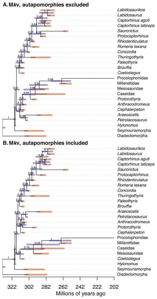
Figure 1: Comparison of the tip-dated phylogenies of early eureptiles inferred when excluding (A) or including (B) autapomorphies, under Mkv ascertainment bias correction.
Numbers are posterior probabilities. Bars represent the 95% HPD.
Inferred node dates
Estimates of the root age are almost identical between analyses with and without autapomorphies (Table 1). Comparing mean dates for nodes shared across the MCC trees yields no significant differences (WSRT, two-sided, n = 14 shared nodes), with P = 0.359 for the Mk inference, and P = 0.280 for Mkv inferences.
Dating uncertainty (HPD widths)
Adding data should reduce uncertainty, especially with small morphological datasets. The null hypothesis, that the no-autapomorphies dataset does not have greater HPD widths, was rejected for the Mk inferences (including vs. excluding autapomorphies, 9.20 vs. 9.94, P = 0.023, one-sided WSRT); the result for the Mkv inferences was only suggestive (9.37 vs. 9.66, P = 0.105).
| Run # | 1 | 2 | 3 | 4 | 5 |
|---|---|---|---|---|---|
| Data | Including autapomorphies | Excluding autapomorphies | |||
| Model | Mk | Mkv | Mk | Mkv | Mk-parsinf |
| Ln posterior | −1393.4 | −1362.2 | −1154.2 | −1144.9 | −1134.4 |
| ESS | 1,801 | 1,485 | 1,801 | 1,801 | 1,801 |
| Root age | 332.6 [330.2, 335.3] | 332.5 [330.0, 335.1] | 332.6 [330.1, 335.1] | 332.6 [330.1, 335.1] | 332.6 [330.0, 335.1] |
| Birth | 0.360 [0.0355, 1.316] | 0.424 [0.0405, 1.708] | 0.342 [0.0463, 1.221] | 0.381 [0.0402, 1.377] | 0.564 [0.0444, 2.841] |
| Death | 0.336 [9.17e−5, 1.315] | 0.3995 [1.13e−4, 1.723] | 0.318 [4.97e−6, 1.220] | 0.357 [2.57e−4, 1.391] | 0.541 [6.37e−4, 2.843] |
| Sampling | 0.0271 [7.90e−4, 0.0626] | 0.0264 [0.00104, 0.0650] | 0.0271 [8.85e−4, 0.063] | 0.0261 [9.96e−4, 0.0634] | 0.0256 [7.66e−4, 0.0643] |
| Clock rate mean | 0.0782 [0.015, 0.159] | 0.0376 [0.0074, 0.0840] | 0.788 [0.0305, 3.982] | 0.550 [0.0228, 2.655] | 0.235 [0.0142, 0.664] |
| Clock rate SD | 1.747 [1.201, 2.399] | 1.712 [1.111, 2.309] | 2.436 [1.572, 3.477] | 2.341 [1.488, 3.379] | 2.079 [1.318, 2.984] |
Posterior probabilities (PPs)
PPs were higher for runs including autapomorphies under both the Mk model (including vs. excluding autapomorphies, 0.902 vs. 0.756) and the Mkv model (0.900 vs. 0.835). The null hypothesis, that the no-autapomorphies dataset does not have smaller PPs, was rejected at a significance level of 0.05 for both the Mk inference (P = 0.0095, one-sided WSRT) and Mkv inference (P = 0.0252).
Relaxed clock
The mean of the relaxed clock rate is dramatically affected by inclusion of autapomorphies, under both the Mk model (with autapomorphies, rate mean = 0.0782 changes per site per million years, 95% HPD [0.015–0.159]; without: 0.788 [0.0305, 3.982]) and the Mkv model (with: 0.0376 [0.0074, 0.0840]; without: 0.550 [0.0228, 2.655]) (tests in Supplemental Information), roughly a increase of an order of magnitude in both cases. The Mkparsinf run of the no-autapomorphies dataset yielded an intermediate clock rate (0.235, 95% HPD [0.0142–0.664]).
Simulations
Figure 2 shows the simulation procedure and key comparisons. Similar tree topologies were inferred under all datasets, but estimated time-branchlengths differed. When the characters are clocklike and autapomorphies are included, inferred time-branchlengths are highly accurate (Fig. 2B). However, when autapomorphies are excluded, inferred terminal branchlengths are biased downwards, and accuracy decreases for all branchlengths. The effect in Fig. 2C can also be seen by comparing inference while including vs. excluding autapomorphies, when the characters are clocklike (Fig. 2D), but this effect disappears for non-clock data (Fig. 2E).

Figure 2: Simulation procedure and results.
Simulation procedure (A) and results (B–E). The lack of an effect of excluding autapomorphies on dating in the empirical eureptile result is similar to the result on non-clock data shown in (E).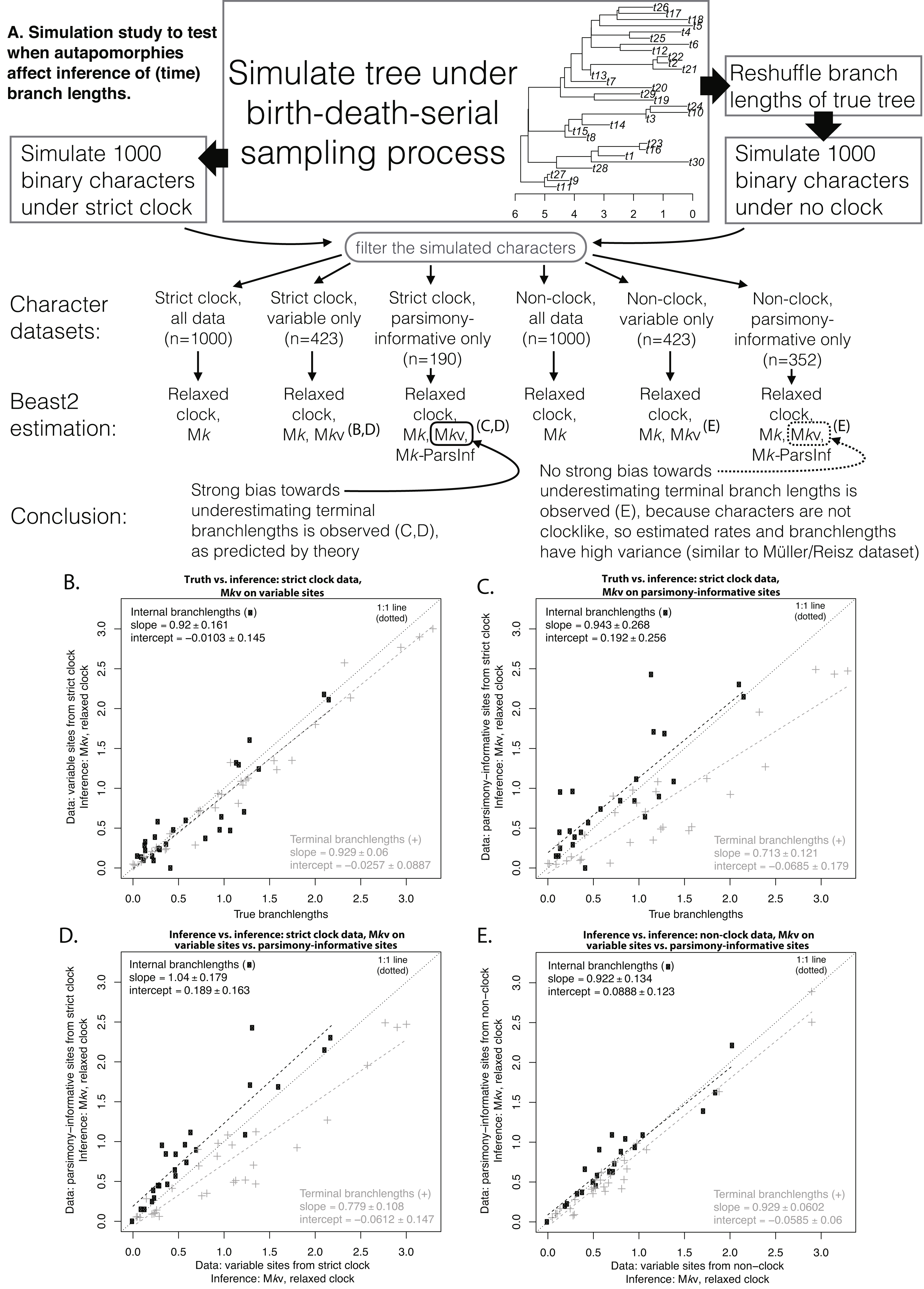
Feasibility of Mkparsinf
Equations in the Appendix demonstrate that Mkparsinf can be feasible for 2-state characters, and for 3-state characters on small datasets (∼10 times slower for our dataset), but rapidly becomes computationally impractical as the number of taxa or states increases. The number of unobservable site patterns for various combinations of numbers of taxa and character states are shown in Table 2.
| # states: 2 | 3 | 4 | 5 | 6 | ||
|---|---|---|---|---|---|---|
| # of taxa | 4 | 10 | 63 | 292 | 1,045 | 3,006 |
| 5 | 12 | 93 | 544 | 2,505 | 9,276 | |
| 10 | 22 | 333 | 4,084 | 42,505 | 381,546 | |
| 20 | 42 | 1,263 | 32,164 | 730,005 | 15,085,086 | |
| 50 | 102 | 7,653 | 500,404 | 30,062,505 | 1,698,527,706 | |
| 100 | 202 | 30,303 | 4,000,804 | 490,250,005 | 57,089,105,406 | |
| 200 | 402 | 120,603 | 32,001,604 | 7,921,000,005 | 1.87E+12 | |
| 500 | 1,002 | 751,503 | 500,004,004 | 3.11E+11 | 1.86E+14 | |
| 1,000 | 2,002 | 3,003,003 | 4,000,008,004 | 4.99E+12 | 5.97E+15 |
Discussion
Although estimated mean rate parameters for the eureptile dataset dropped dramatically (by 10 times or more) when autapomorphies were included (and somewhat less when ascertainment-bias correction was used instead), the downstream effects on confidence were small (Table 1; Supplemental Information), and there was no detectable effect on date inference. This seems surprising, because the exclusion of autapomorphies must reduce the number of morphological changes on terminal branches. However, reflection on the interaction between non-clocklike data, and the flexibility of relaxed-clock Bayesian tip-dating methods, provides an explanation. If the character data are non-clocklike, then the method will estimate a high rate of branchwise rate variation, indicating lack of correlation between time elapsed and morphological branchlength. In this situation, most of the dating information for the analysis comes from the serial-sampling of fossil tips rather than morphological branchlengths. If morphological branchlength is not correlated with time, this remains true whether or not autapomorphies are included, and adding autapomorphies is not likely to change the dating inference.
Our simulation results (Fig. 2) confirm this explanation. The analysis of the empirical eureptile dataset is likely similar to the situation shown in Fig. 2E: inferred time branchlengths are roughly the same whether or not autapomorphies are included. However, on a clocklike dataset, exclusion of autapomorphies clearly has an effect (Fig. 2C). This suggests that the importance of including autapomorphies in tip-dating analyses depends on whether or not the characters have clocklike behavior. Unfortunately, assessing clocklike behavior will be more difficult when autapomorphies have been ignored or gathered only inconsistently (as is common).
An alternative to coding autapomorphies is the Mkparsinf model. However, the Appendix shows that it scales too poorly to be generally useful for characters with large number of states (Table 2; Supplemental Information). All versions of MrBayes back to at least 3.1.2 allow a “coding=informative” ascertainment bias correction to be specified, but the increase in computation time for a run with a single discrete character is very similar whether the character has 2, 3, 4, or 5 states (tested on MrBayes versions 3.1.2 through 3.2.6, and the 3.2.7 development version). This suggests that Mkparsinf may be implemented assuming only binary characters, and may be formally incorrect for multistate characters (as briefly noted by Dos Reis, Donoghue & Yang, 2016; Matzke, 2016), despite many usages in the literature. However, as most morphological datasets are dominated by binary characters, this issue may have limited impact on inference, and requires further study.
Conclusion
Our study indicates that the common practice of repurposing character matrices devised for parsimony and undated Bayesian analyses may not be sufficient in the world of Bayesian tip-dating. For higher quality datasets (many characters, clocklike behavior), the bias in dating introduced by ignoring autapomorphies may become significant. Additionally, ascertainment bias corrections are at present computationally impractical for many datasets with multistate characters. Finally, autapomorphies have additional utility for improving estimates of rates and rate variation, for species identification, for measuring disparity, and because autapomorphies may become synapomorphies when new taxa are described. Therefore, we recommend that autapomorphies be coded and used whenever possible.