
Machine-learning-based automated quantification machine for virus plaque assay counting
- Published
- Accepted
- Received
- Academic Editor
- Shawn Gomez
- Subject Areas
- Bioinformatics, Computational Biology, Autonomous Systems, Computer Vision, Robotics
- Keywords
- K-mean clustering, Image segmentation, Optical inspection, Viral plaque assay, Virus titer, Well plate
- Copyright
- © 2022 Phanomchoeng et al.
- Licence
- This is an open access article distributed under the terms of the Creative Commons Attribution License, which permits using, remixing, and building upon the work non-commercially, as long as it is properly attributed. For attribution, the original author(s), title, publication source (PeerJ Computer Science) and either DOI or URL of the article must be cited.
- Cite this article
- 2022. Machine-learning-based automated quantification machine for virus plaque assay counting. PeerJ Computer Science 8:e878 https://doi.org/10.7717/peerj-cs.878
Abstract
The plaque assay is a standard quantification system in virology for verifying infectious particles. One of the complex steps of plaque assay is the counting of the number of viral plaques in multiwell plates to study and evaluate viruses. Manual counting plaques are time-consuming and subjective. There is a need to reduce the workload in plaque counting and for a machine to read virus plaque assay; thus, herein, we developed a machine-learning (ML)-based automated quantification machine for viral plaque counting. The machine consists of two major systems: hardware for image acquisition and ML-based software for image viral plaque counting. The hardware is relatively simple to set up, affordable, portable, and automatically acquires a single image or multiple images from a multiwell plate for users. For a 96-well plate, the machine could capture and display all images in less than 1 min. The software is implemented by K-mean clustering using ML and unsupervised learning algorithms to help users and reduce the number of setup parameters for counting and is evaluated using 96-well plates of dengue virus. Bland–Altman analysis indicates that more than 95% of the measurement error is in the upper and lower boundaries [±2 standard deviation]. Also, gage repeatability and reproducibility analysis showed that the machine is capable of applications. Moreover, the average correct measurements by the machine are 85.8%. The ML-based automated quantification machine effectively quantifies the number of viral plaques.
Introduction
A plaque assay is one of the standard measurements (Dulbecco, 1952) for viable viruses in virology laboratories. Applications of this method range from basic research through drug discovery to vaccine development (Premsattham et al., 2019). In principle, viruses infect the cell monolayer in a semisolid medium, thus limiting only the horizontal spread. The area of cell death (i.e., plaque) is visualized under a microscope before staining with neutral red or crystal violet (BioTek Instruments, Inc, 2021; Cacciabue, Currá & Gismondi, 2019). The plate is manually counted and calculated to quantify the virus. The manual counting of plaques is tedious and requires well-trained personnel for verification. The plaque assay can be performed in low to medium throughput formats, such as 6-, 12-, or 24-well plates. This method requires more reagents and highly skilled operators to appropriately perform the assay. Recently, a simplified microwell plaque titration assay was developed with Herpes simplex (Bhattarakosol, Yoosook & Cross, 1990) and dengue viruses (Boonyasuppayakorn et al., 2016). Automated data acquisition and quantification methods have been developed under a flatbed scanner (Boonyasuppayakorn et al., 2016; Sullivan et al., 2012).
Recently, automated imaging-based counters have been applied to plaque assays; however, the current versions face multiple challenges. For example, Cellular Technology Limited developed a commercial Elispot and viral plaque-counting machine called ImmunoSpot CLT Analyzers (Cellular Technology Ltd., Shaker Heights, OH, USA). The machines can automatically acquire high-resolution images for each well plate with a high speed and automatically count plaque using software. Even though the software focuses on counting Elispot assays the company can optimize the setup, such as plaque intensity and size to develop programs for counting viral plaques for each well plate (Smith et al., 2013; Sukupolvi-Petty et al., 2013). However, the program has limitations: it cannot be easily optimized and standardized for various viral plaques. Moreover, commercial machines and their services are often expensive and proprietary.
For plaque counting on a personal computer, general image-processing tools, such as ImageJ, OpenCV, Labview, R, have been employed (Boonyasuppayakorn et al., 2016; Rasband, 1997-2015; R Core Team, 2016; Cai et al., 2011; Cacciabue, Currá & Gismondi, 2019; Geissmann, 2013; Katzelnick et al., 2018; Moorman & Dong, 2012). Boonyasuppayakorn et al. (2016) developed an ImageJ program and employed it for a modified 96-well plaque assay for the dengue virus. A flatbed scanner was used in the assay to acquire the 96-well plate image before cropping it into each well image. However, the plate must be contrast-enhanced by adding nontransparent liquid, such as milk, before scanning, which increases the workload. Work in several studies (Cai et al., 2011; Cacciabue, Currá & Gismondi, 2019; Geissmann, 2013; Katzelnick et al., 2018; Moorman & Dong, 2012) have developed programs to count viral plaque based on image segmentation, morphological analysis, and image threshold, but the programs require image-processing knowledge to implement and may not be suitable for some assays. To date, no machine learning (ML)-based program has been developed for plaque counting.
Due to the need of reducing the number of staff that conduct viral plaque assay, we developed an automated quantification machine based on ML. The machine comprises the hardware system for image acquisition and ML-based software for image viral plaque counting. The hardware is relatively simple to set up, affordable, portable, and automatically acquires a single image or multiple images from a multiwell plate for users. The software is implemented using K-mean clustering, which is a ML algorithm and unsupervised learning algorithm to help users. The algorithm helps by reducing the number of setup parameters for counting.
The automated quantification machine was built and evaluated with 96-well plates of dengue virus. The processes for standardizing the manual and software counting algorithm and evaluating the performance of the system on several plaque images are described in the next section. The counting results from the machine are consistent with those from manual counting.
Materials & Methods
Cell and viruses
Simplified dengue microwell plaque assays were performed following the procedure reported in Boonyasuppayakorn et al. (2016). In summary, the 10-fold serially diluted viruses in a maintenance medium to 10−6 were used as the reference. LLC/MK2 (ATCC®CCL-7) cells at 1 × 10⁴ cells per well (50 µl) of a 96-well plate were mixed with all dilutions and undiluted samples.
Then, the dilution was prepared and the cells were incubated as explained in Boonyasuppayakorn et al. (2016). Finally, the dengue virus cells were fixed and then stained as the standard assay. The number of plaque-forming units (p.f.u.) per ml was determined manually and using the automated quantification machine for evaluation.
Automated quantification machine
The automated quantification machine was developed to acquire viral plaque images of each well plate and automatically display the counting results in an easy-to-use manner. The major components of the machine are the hardware for image acquisition and ML-based software for image viral plaque counting.
Hardware for image acquisition
The automated quantification machine was developed to reduce workload and enable personal use in laboratories. Thus, the machine is relatively simple to set up, affordable, portable, and automatically acquires single or multiple images from multiwell plates for users. Then, the hardware components of the machine include an IAI Tabletop, Model TT-A3-I-2020-10B-SP (IAI Robot (Thailand) Co., Ltd., Bangkok Thailand), a USB microscope camera, Dino-Lite AM4113T (AnMO Electronics Corporation, Hsinchu, Taiwan), and an adjustable light source panel, 150 mm × 150 mm surface LED illumination source.
A photo and a schematic of the automated quantification machine are shown in Figs. 1A and 1B, respectively. The IAI Tabletop is a 3-axis Cartesian robot with a working space of 200 mm × 200 mm × 100 mm (x-, y-, and z-axis). Its repeating positioning accuracy is less than ± 0.02 mm. The x-axis of the IAI Tabletop is installed with the multiwell plate fixture and the light source panel and the z-axis is installed with a camera holder and a USB microscope camera. With the Cartesian robot configuration, the IAI Tabletop can move a multiwell plate along the x–y plane for automatic and accurate positioning to capture the well images with the USB microscope camera and move the USB microscope camera along the z-axis to automatically focus the image.
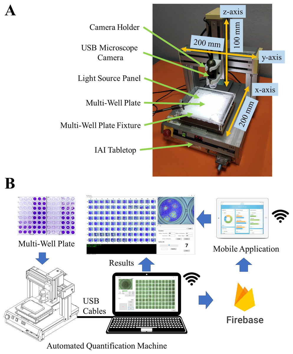
Figure 1: Automated quantification machine.
(A) Prototype of automated quantification machine. (B) Schematic of automated quantification machine.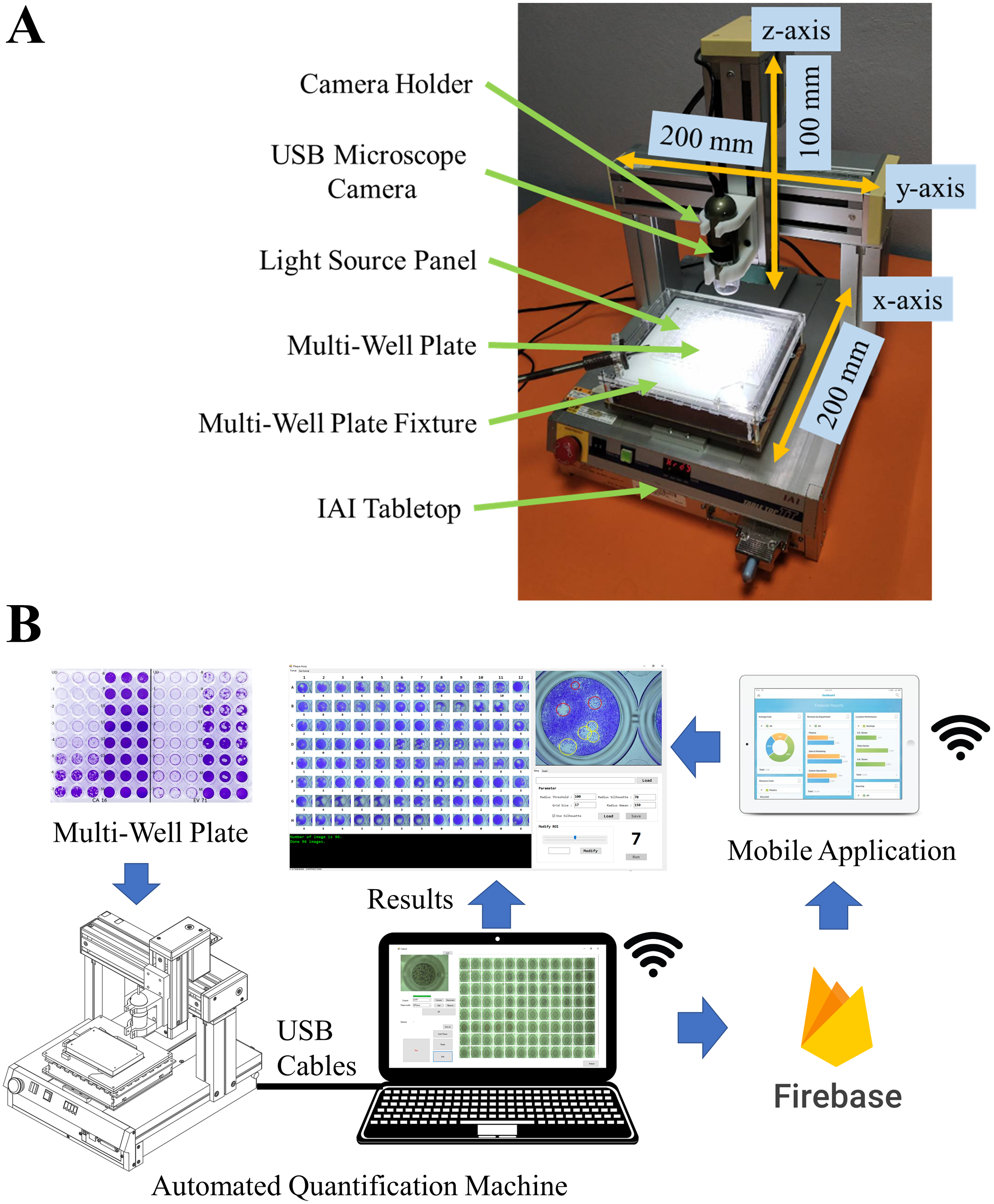
The USB microscope camera is a color camera with a resolution of 1280 × 1024 pixels and 10×–50 ×, 220 × magnification range. It is equipped with an LED coaxial light source. With low magnification, the camera can capture a full-size well image of a six-well plate, and with medium magnification, the camera can capture a full-size well image of a ninety-six-well plate. To change the magnification of the camera, the magnification ring is manually adjusted.
The adjustable light source panel is a square surface LED illumination source. It is installed on the x-axis of the IAI Tabletop and underneath the multiwell plate fixture. The light source panel has high parallelism of light. The high parallelism of the light source panel renders the object edges clearer and sharper in an image. For viral plaque counting, the back-light technique is employed since it gives better image quality than the bright- and dark-field techniques. The back-light technique can be performed by turning off the LED coaxial light source and turning on the light source panel.
To control the machine hardware, the hardware is connected to a personal computer via USB cables and is controlled by a window application developed using C# language. The window application communicates to the IAI Tabletop by PSEL protocol to control the position of the multiwell plate. It also communicates to the USB microscope camera by DNVIT SDK to control the coaxial light source and image acquisition. Images are saved in PNG format. The user interface and user experience (UI/UX) design was considered in creating the window application. The window application consists of 1. calibration routine 2. single image and multiwell plate image acquisition 3. Google Firebase database (https://firebase.google.com).
The calibration routine is used to calibrate the movement of the IAI Tabletop. A screenshot of the calibration control is shown in Fig. 2A. Due to the installation process, the coordinate of the multiwell plate fixture is not the same as the coordinate of the IAI Tabletop. This causes the misalignment of the well center position when capturing an image. To apply the calibration routine, the user can work in two steps. The first step is to control the IAI Tabletop by UI control to locate the A1, A12, and H1 well center positions, as shown in Fig. 2A. The second step is to click the calibration routine button. Then, the algorithm automatically recalculates the new coordinate of the IAI Tabletop and makes the coordinate of the multiwell plate fixture and IAI Tabletop the same.
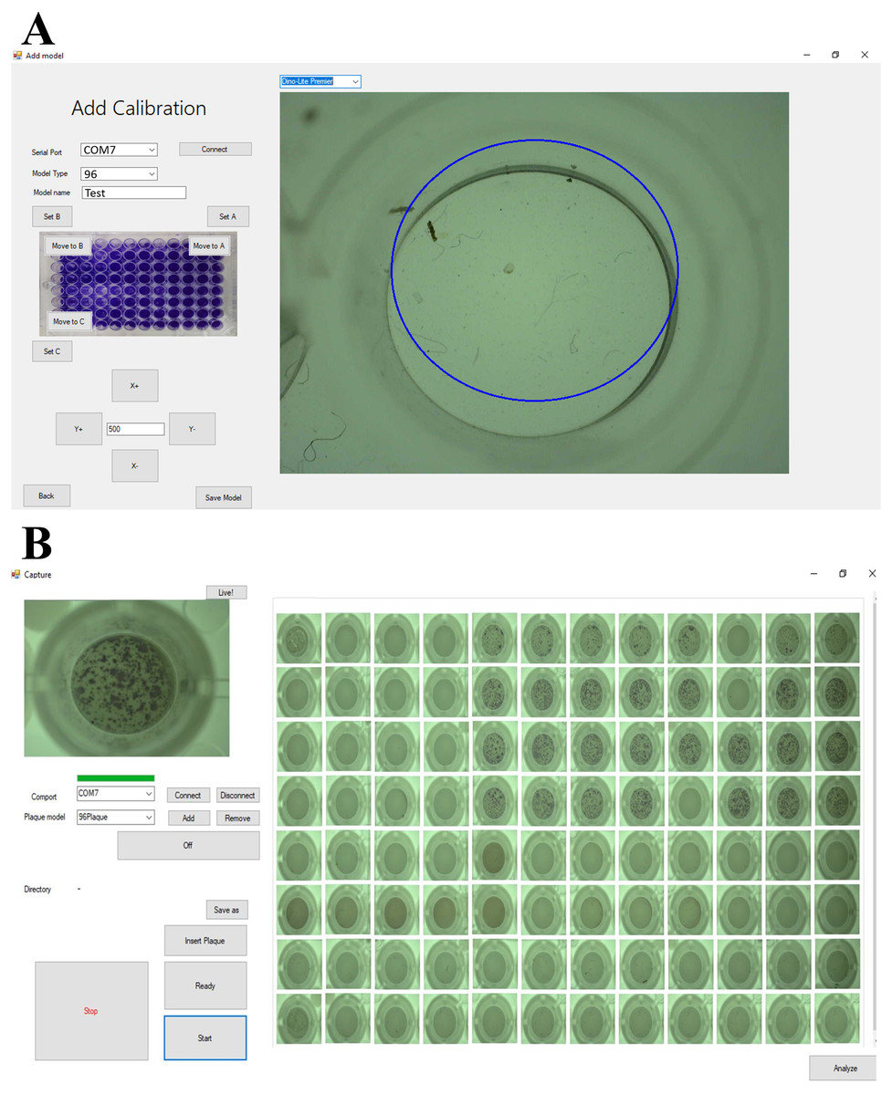
Figure 2: Screenshot of calibration control and image acquisition control.
(A) Calibration control. (B) Image acquisition control.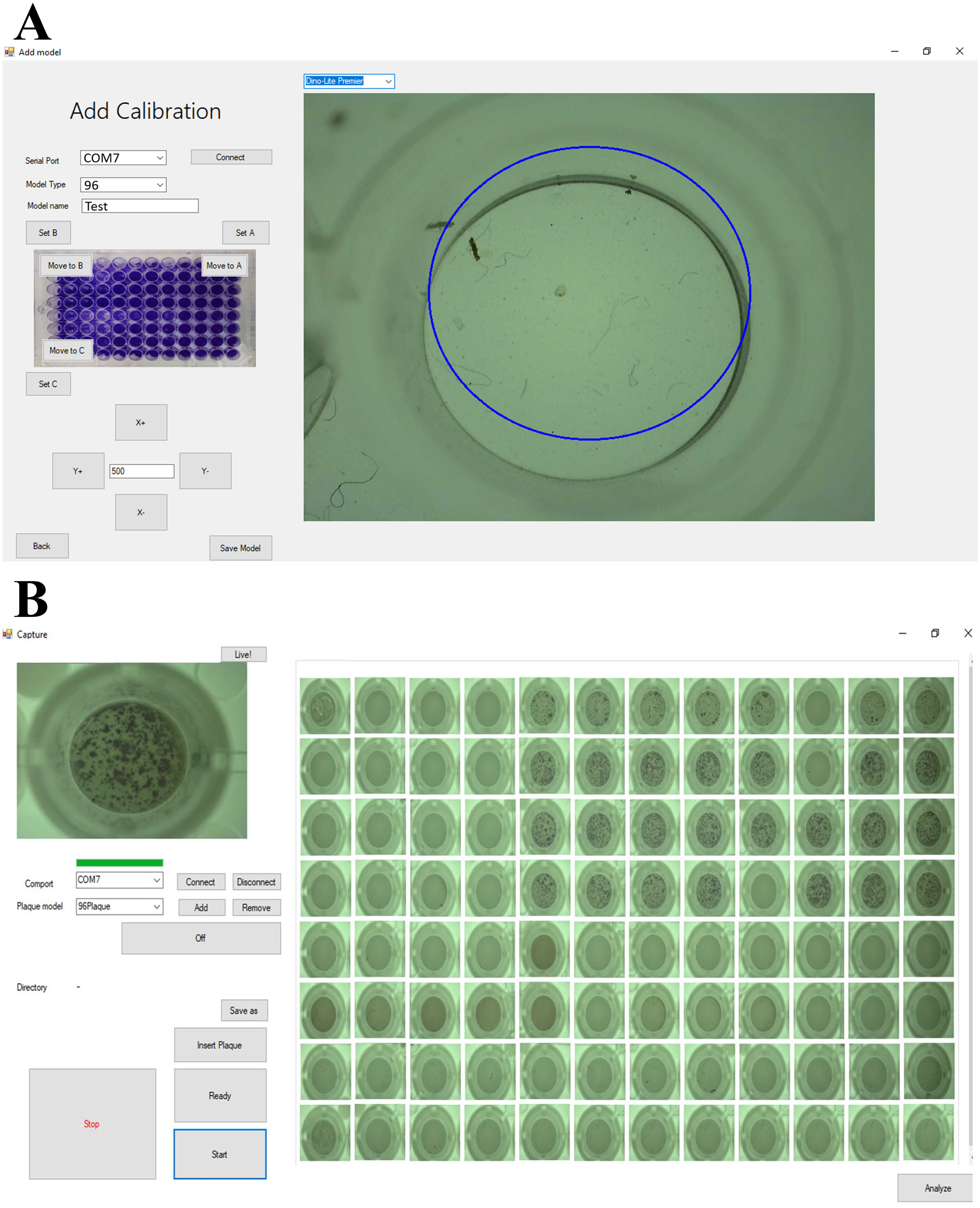
The single and multiwell plate image acquisition allows the user to select how to acquire well images. A screenshot of the image acquisition control is shown in Fig. 2B. With the single image acquisition, the user only selects or keys in the desired well number, such as A1, B2, and H12. Then, the machine moves, captures, and displays the desired well image. Moreover, with the multiwell plate image acquisition, the user only clicks one button to make the machine automatically capture and display all multiwell plates. For the 96-well plate, the machine can capture and display all images within less than 1 min. Once images are captured, the user may use the ML-based software for image viral plaque counting.
The Firebase database is used to collect all results of the machine for backup. The data in the Firebase database allows new features of the machine to be developed in the future, such as the data storage and exploration features, data analysis tools, data dashboard, web applications, and remote operation. These will provide greater convenience to users.
Machine learning software for image viral plaque counting
The algorithm for image viral plaque counting is ML and K-mean clustering (Arora & Varshney, 2016). It helps users and reduces the number of setup parameters for counting. The algorithm is also implemented in a Windows application developed by visual studio C# language and image-processing library, (MVtec Halcon MVTec Software GmbH, Munich, Germany; MVTec Software GmbH, 2021a).
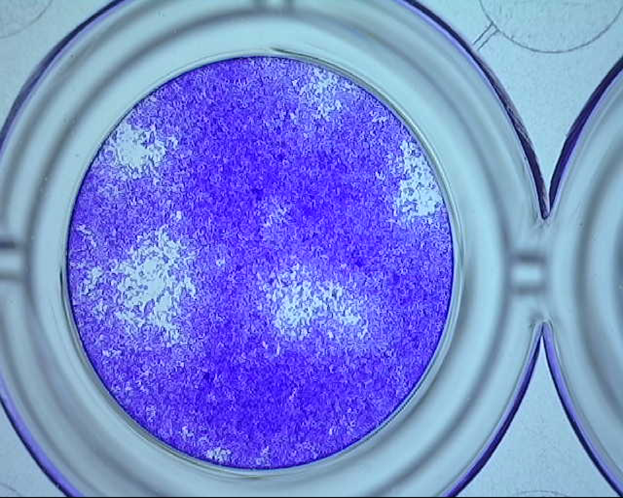
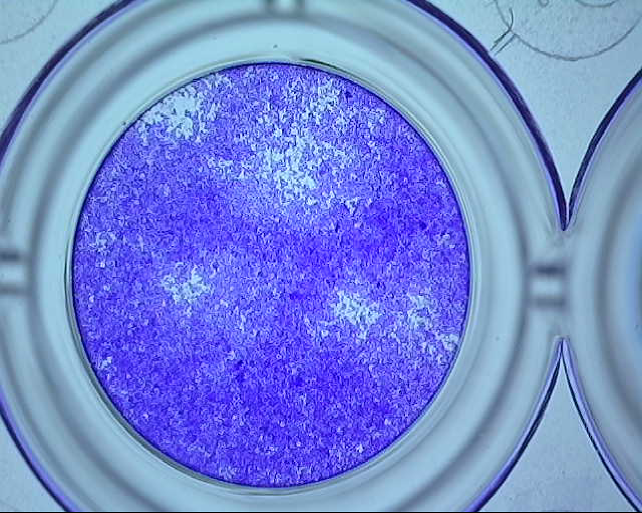
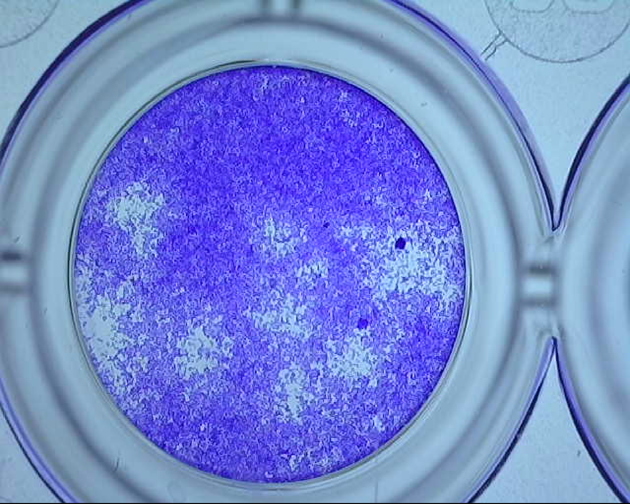
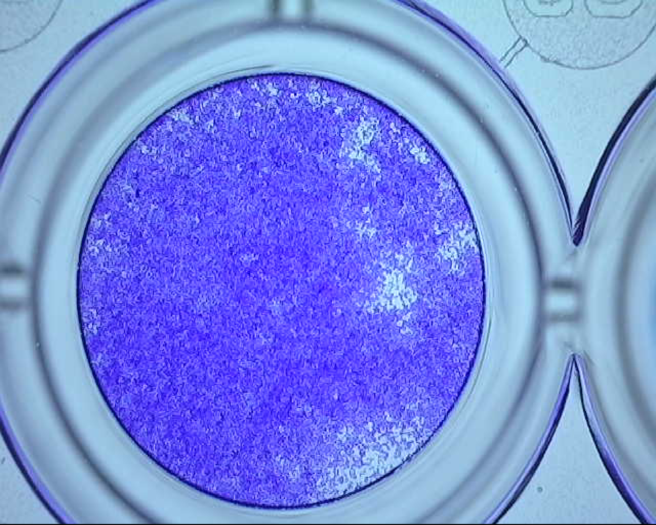
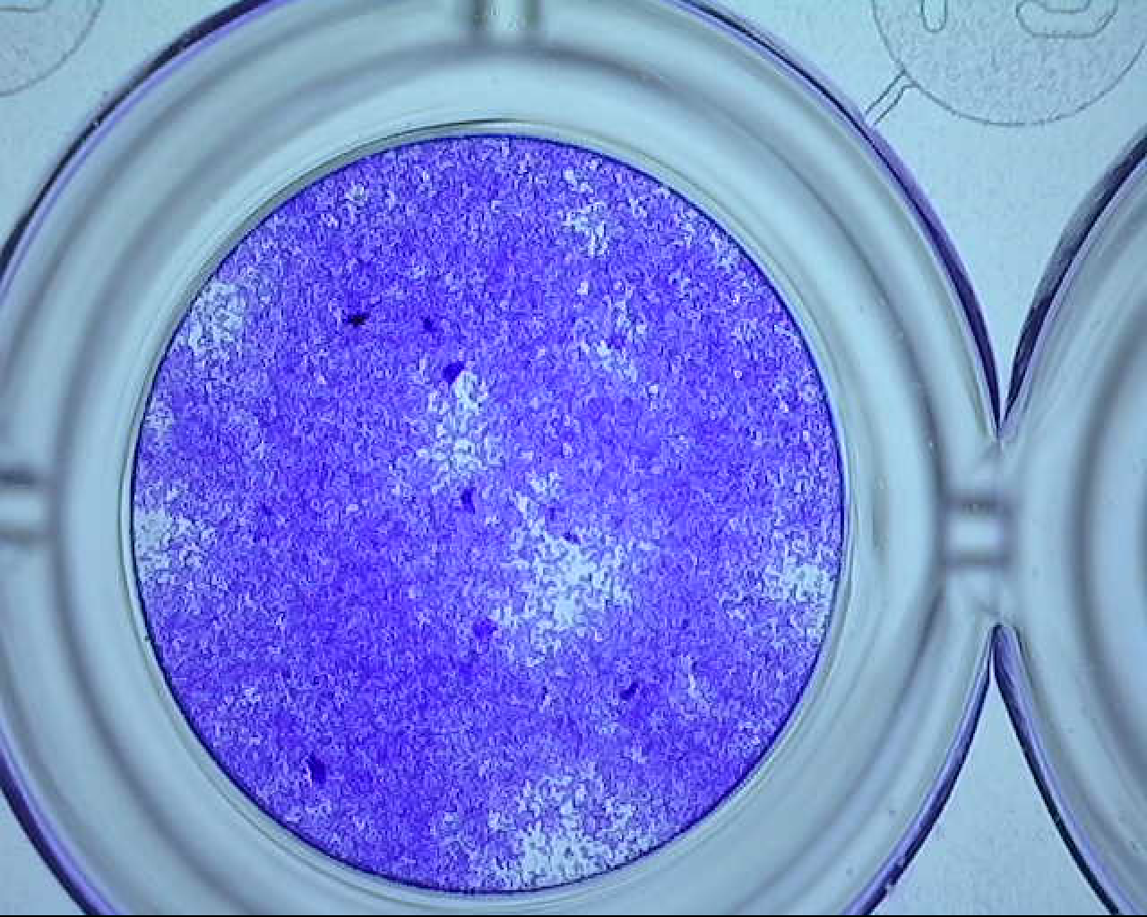
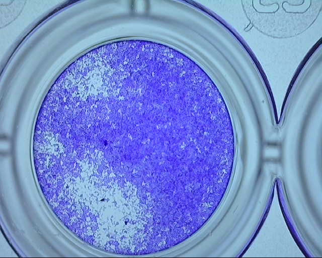
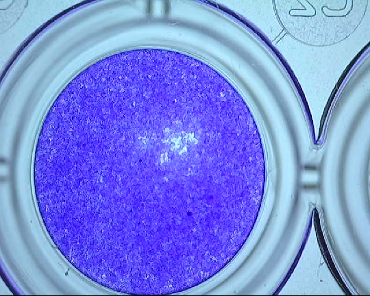
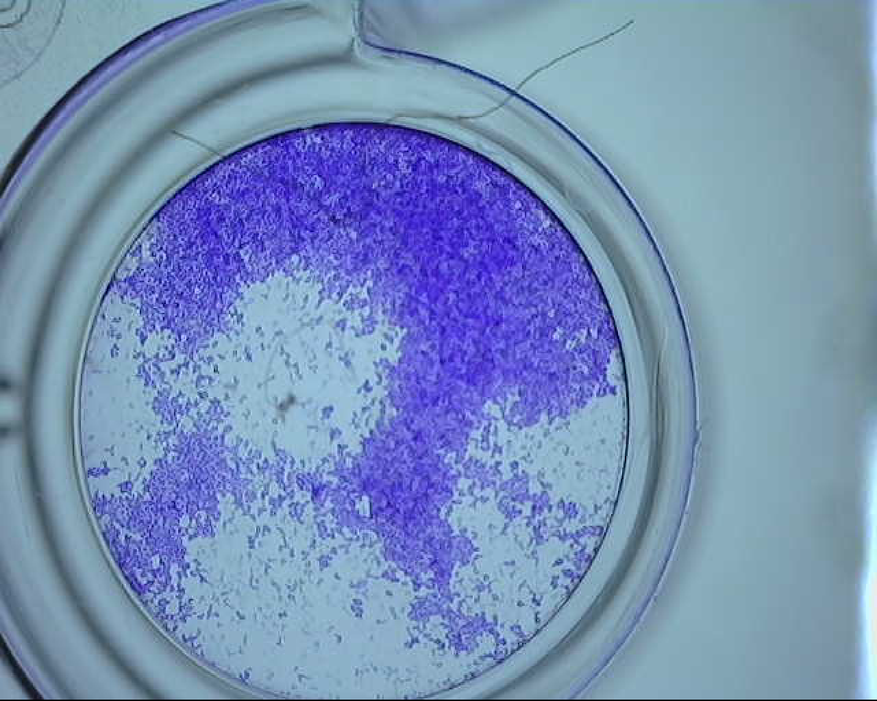
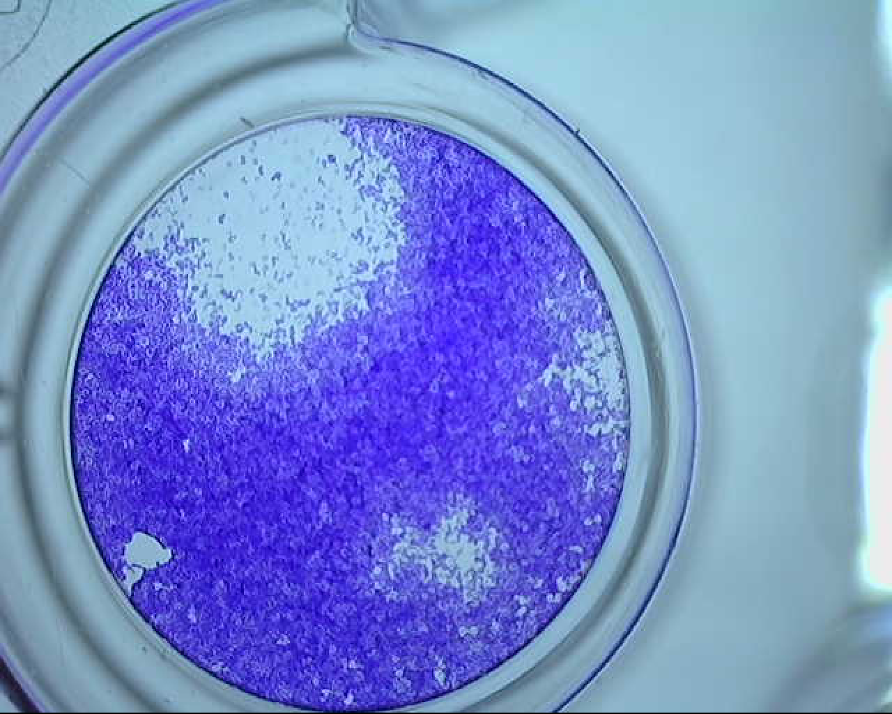
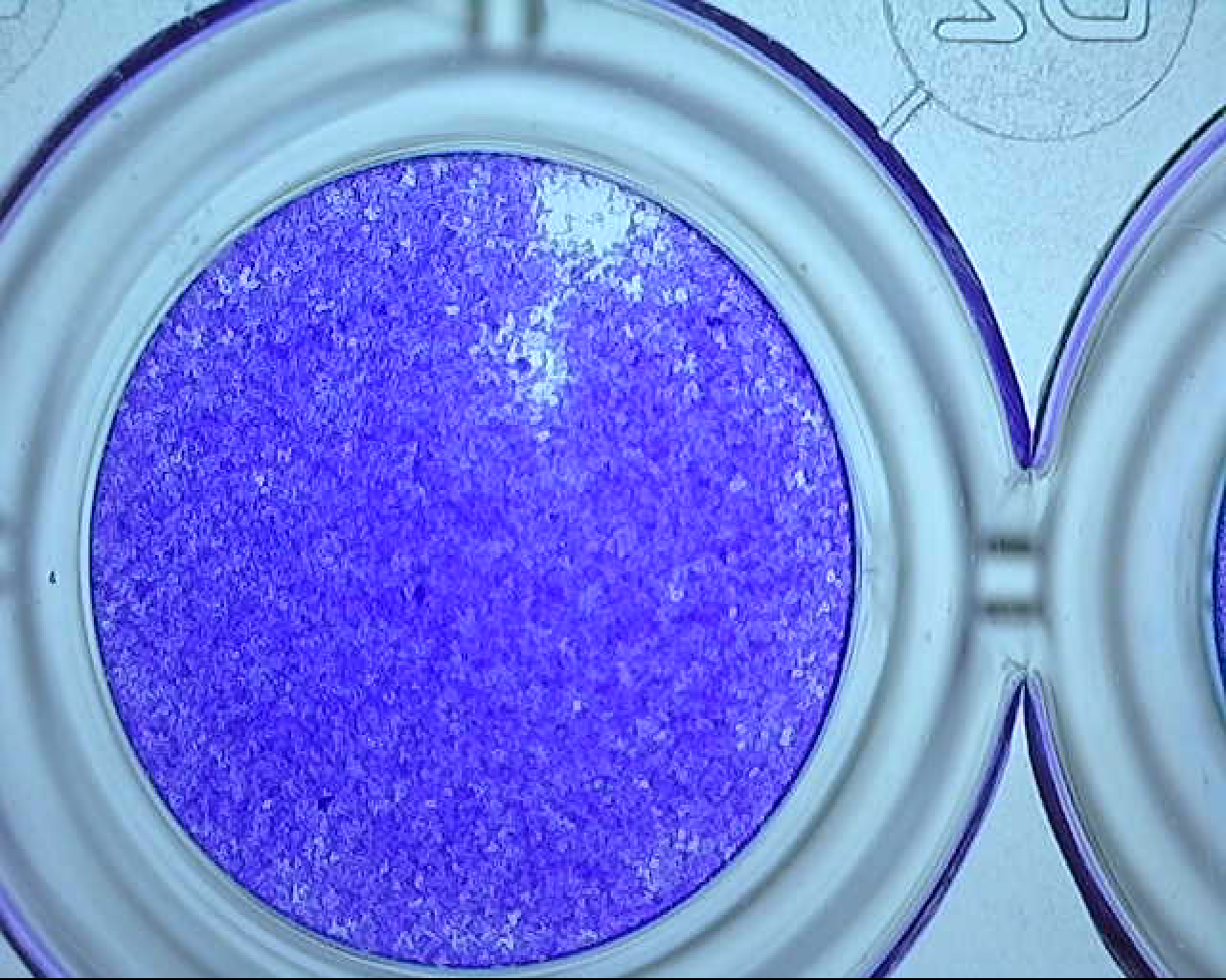
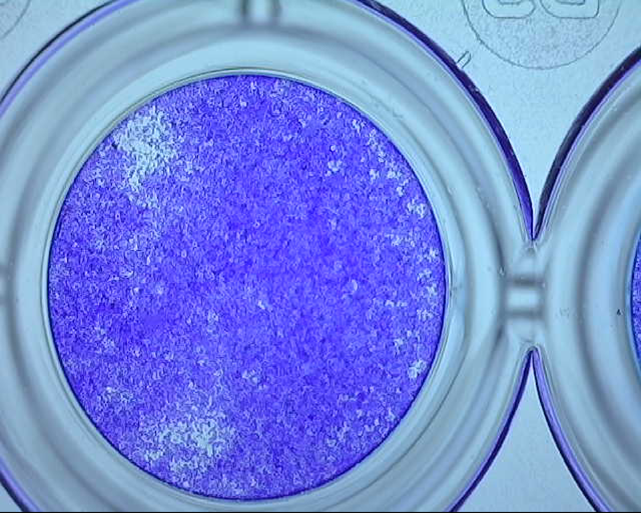
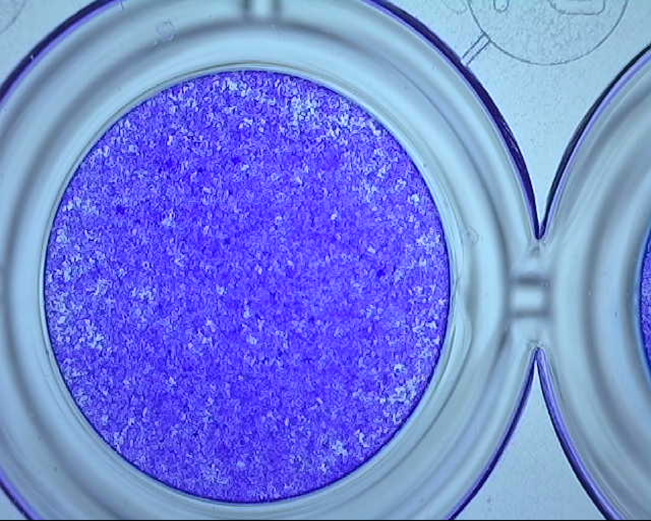
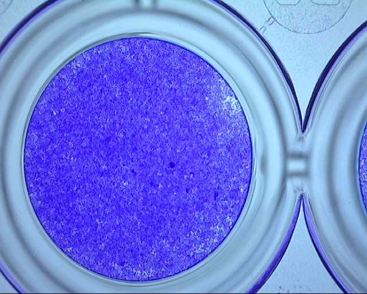
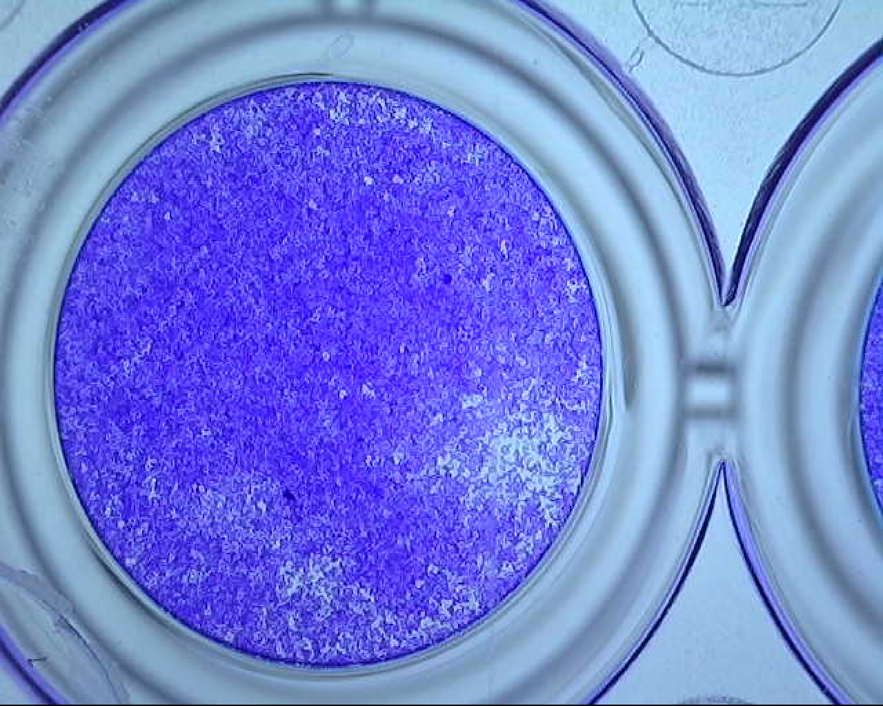
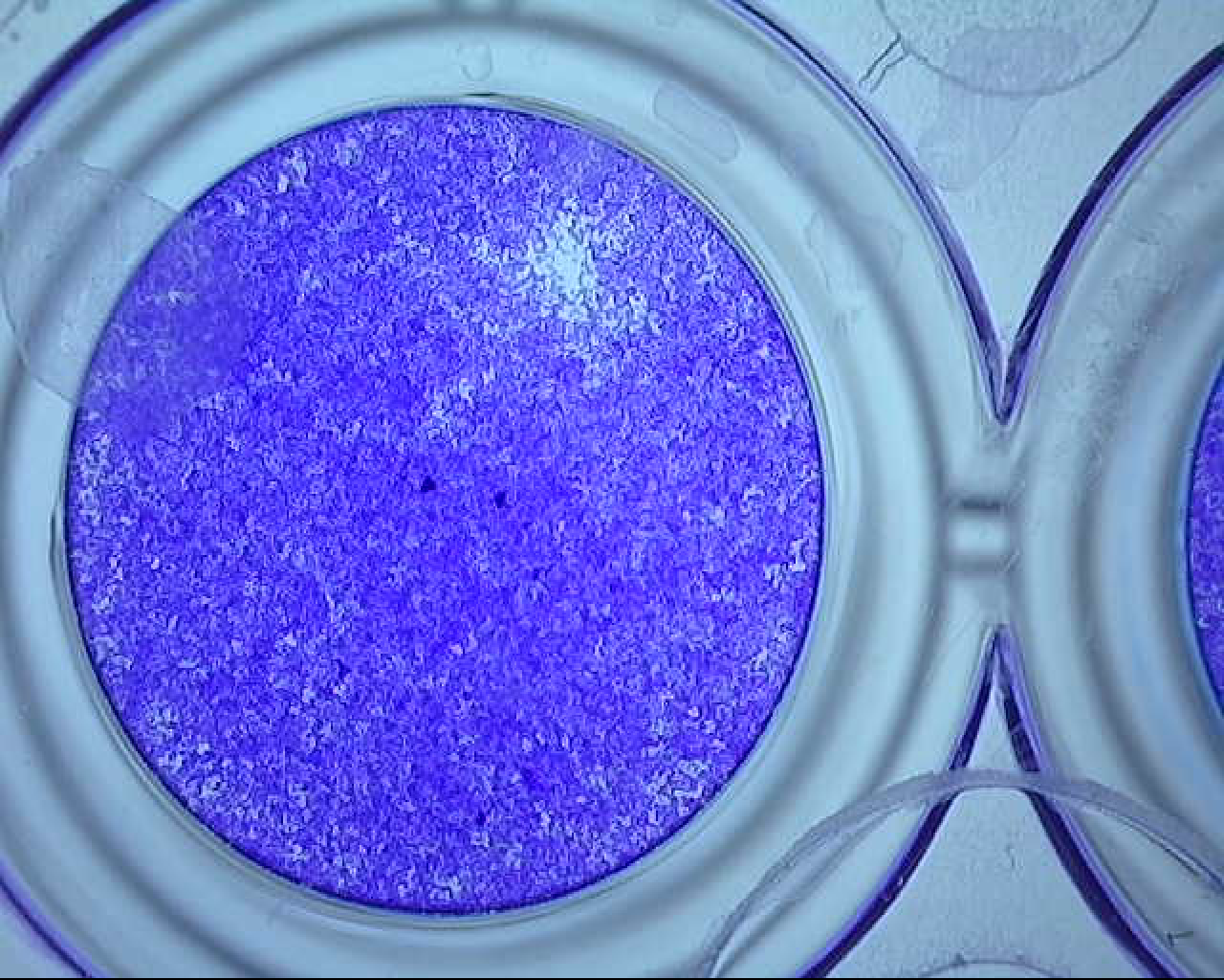
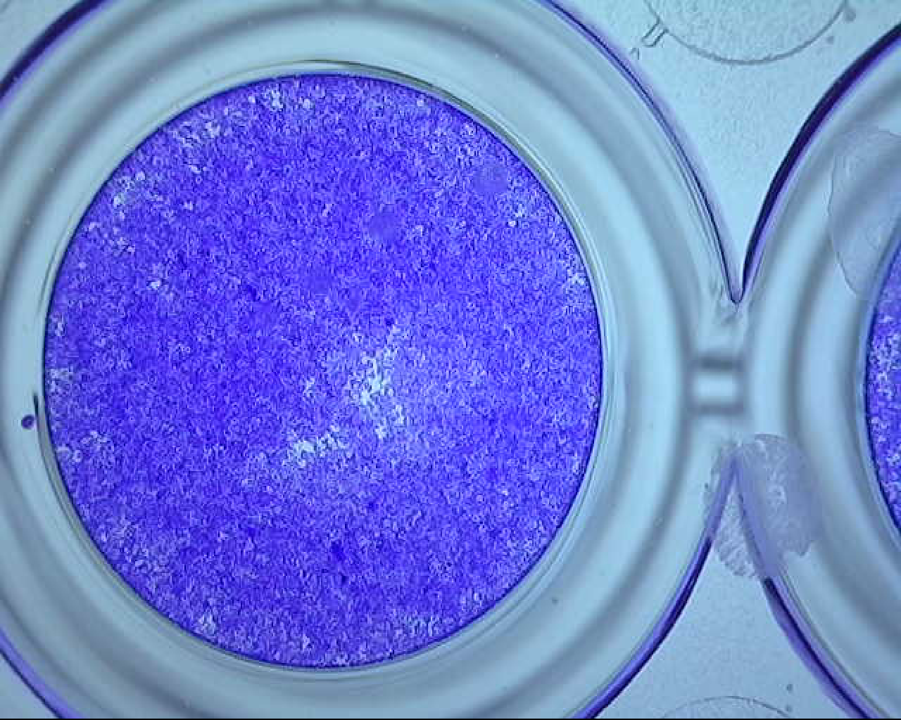
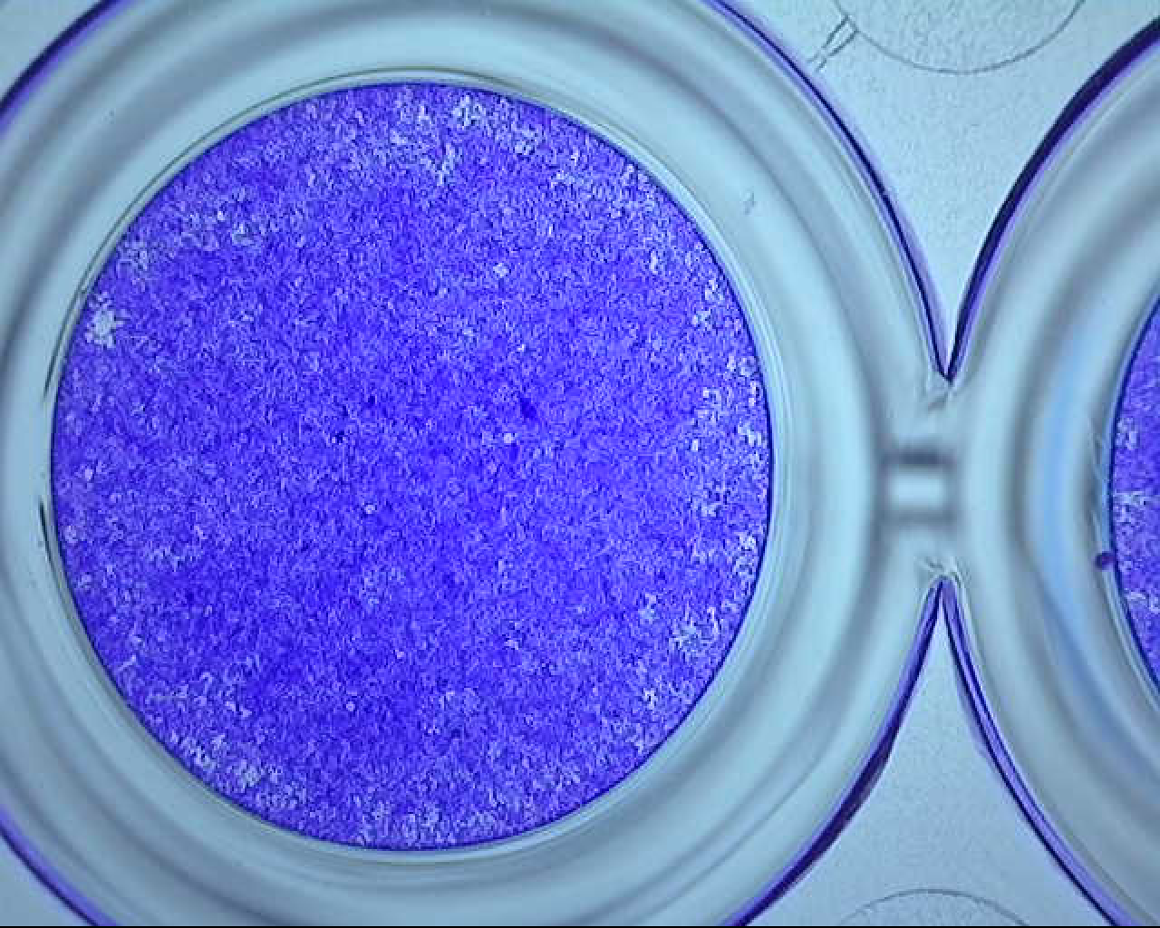
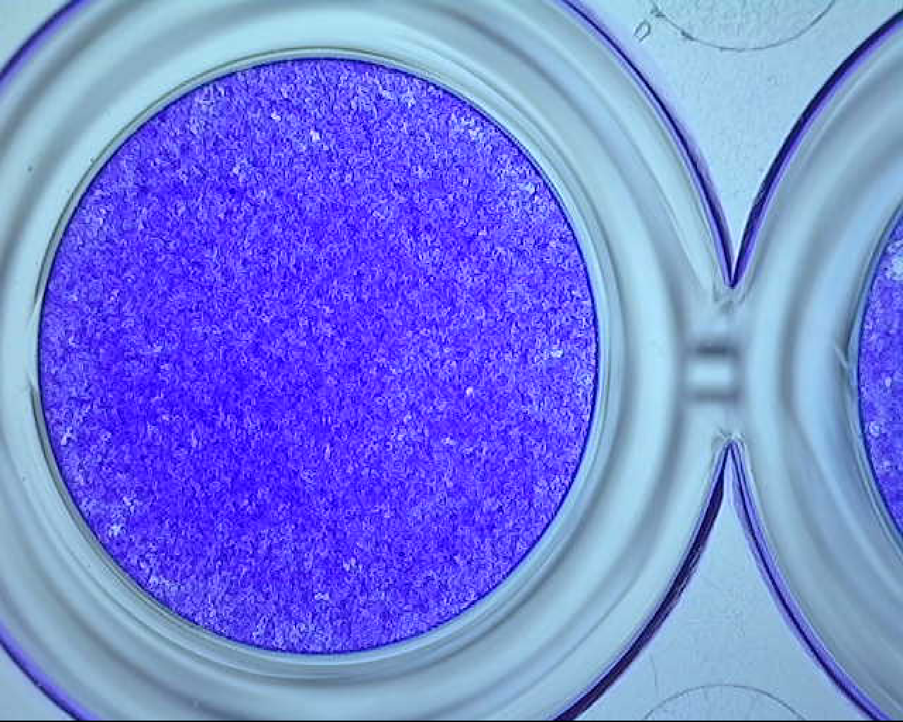
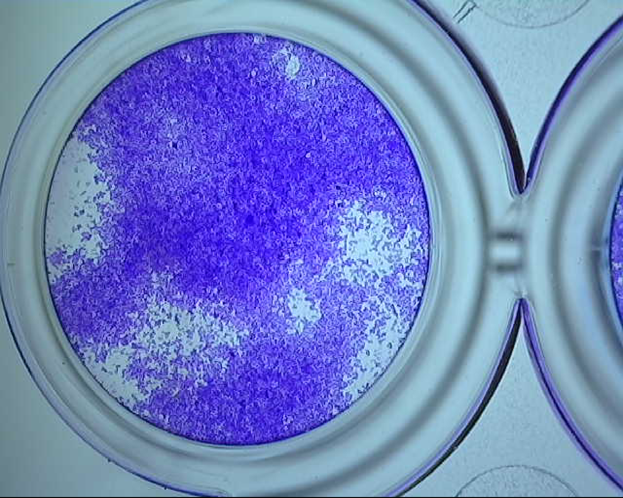
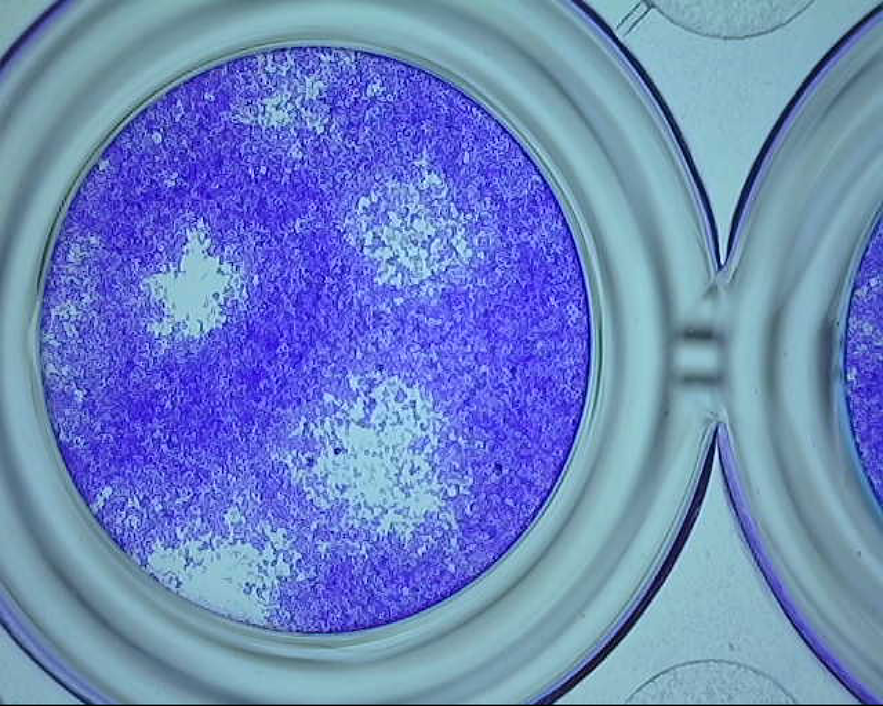
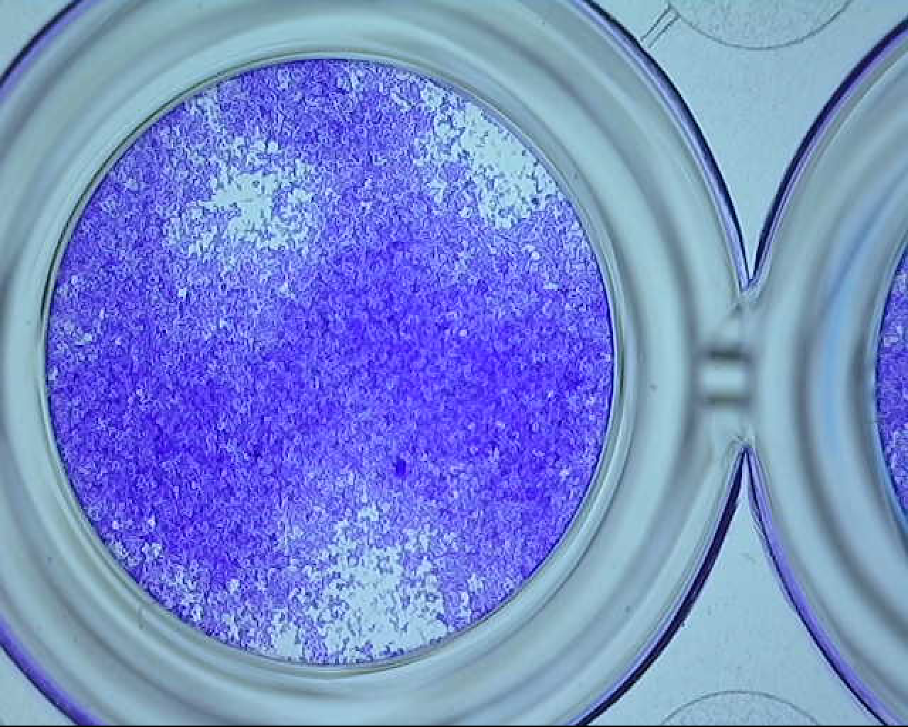
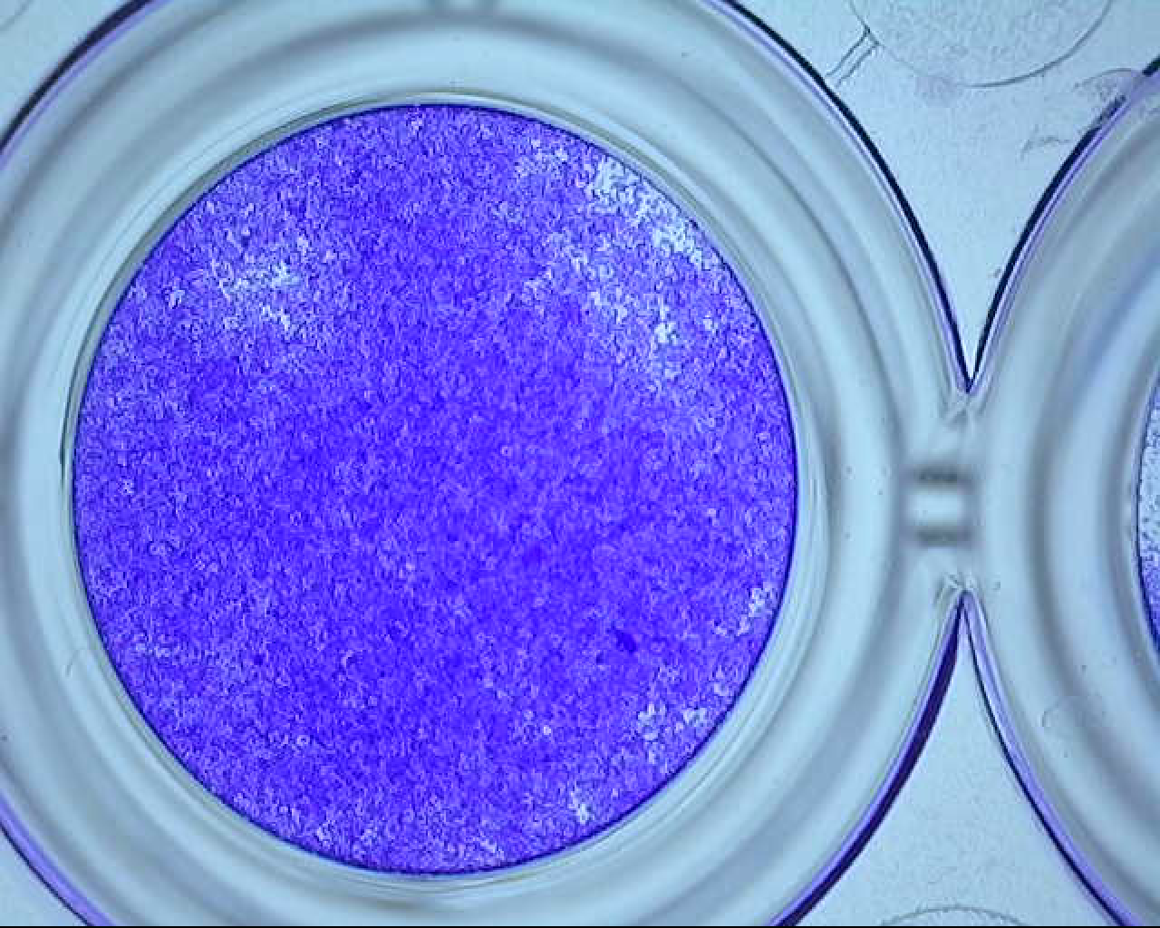
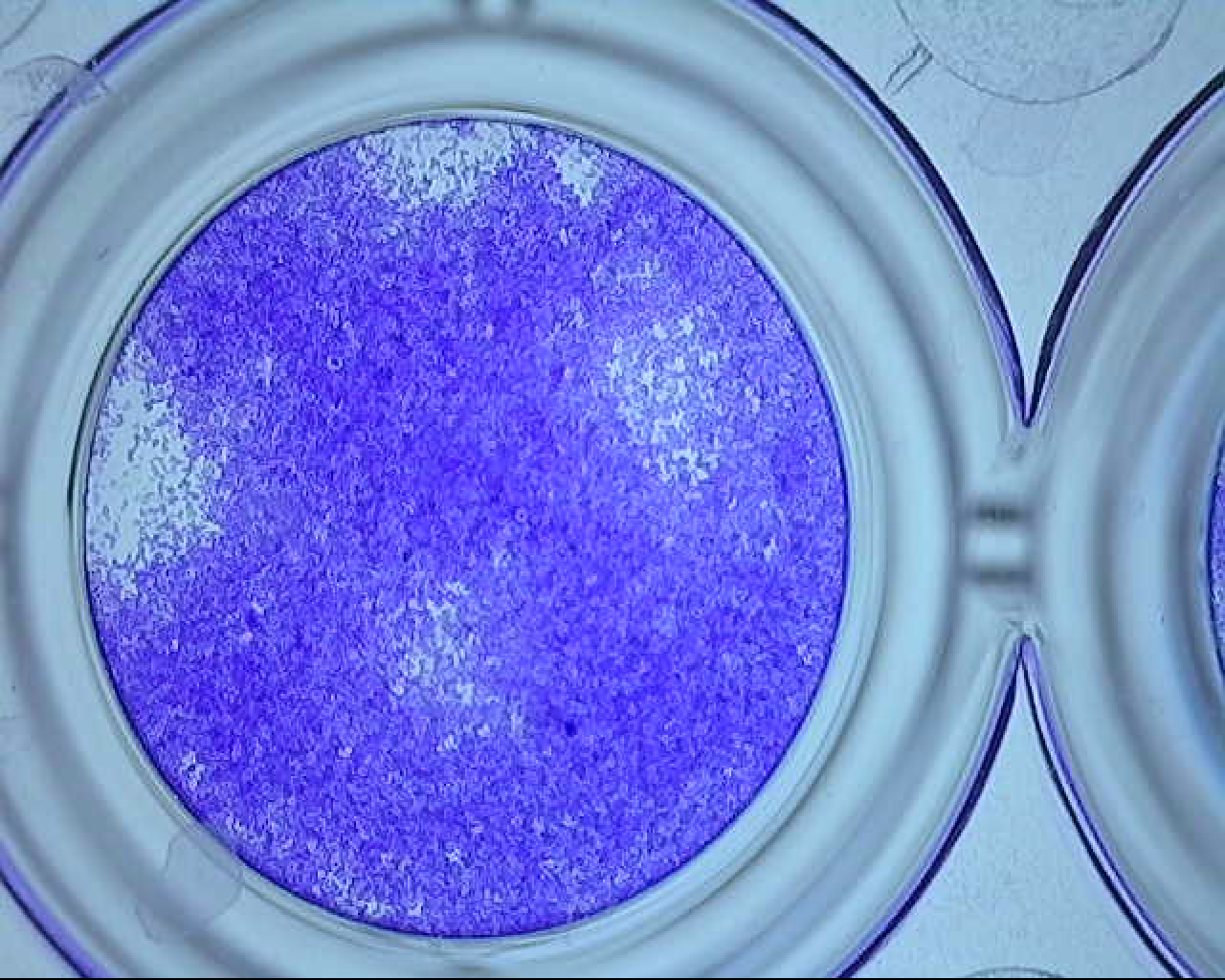
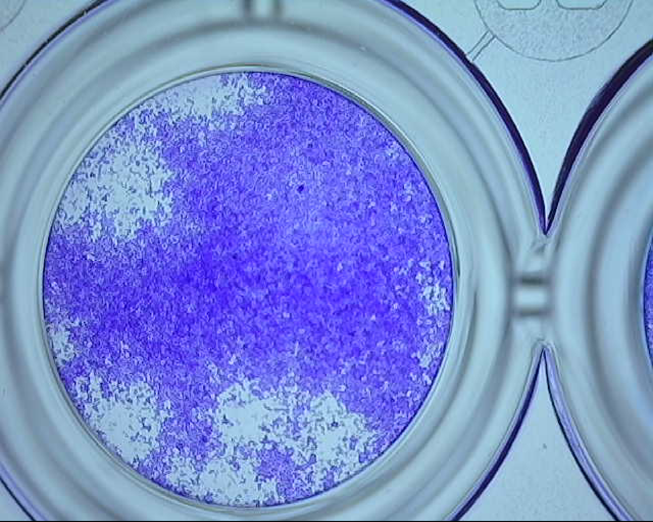
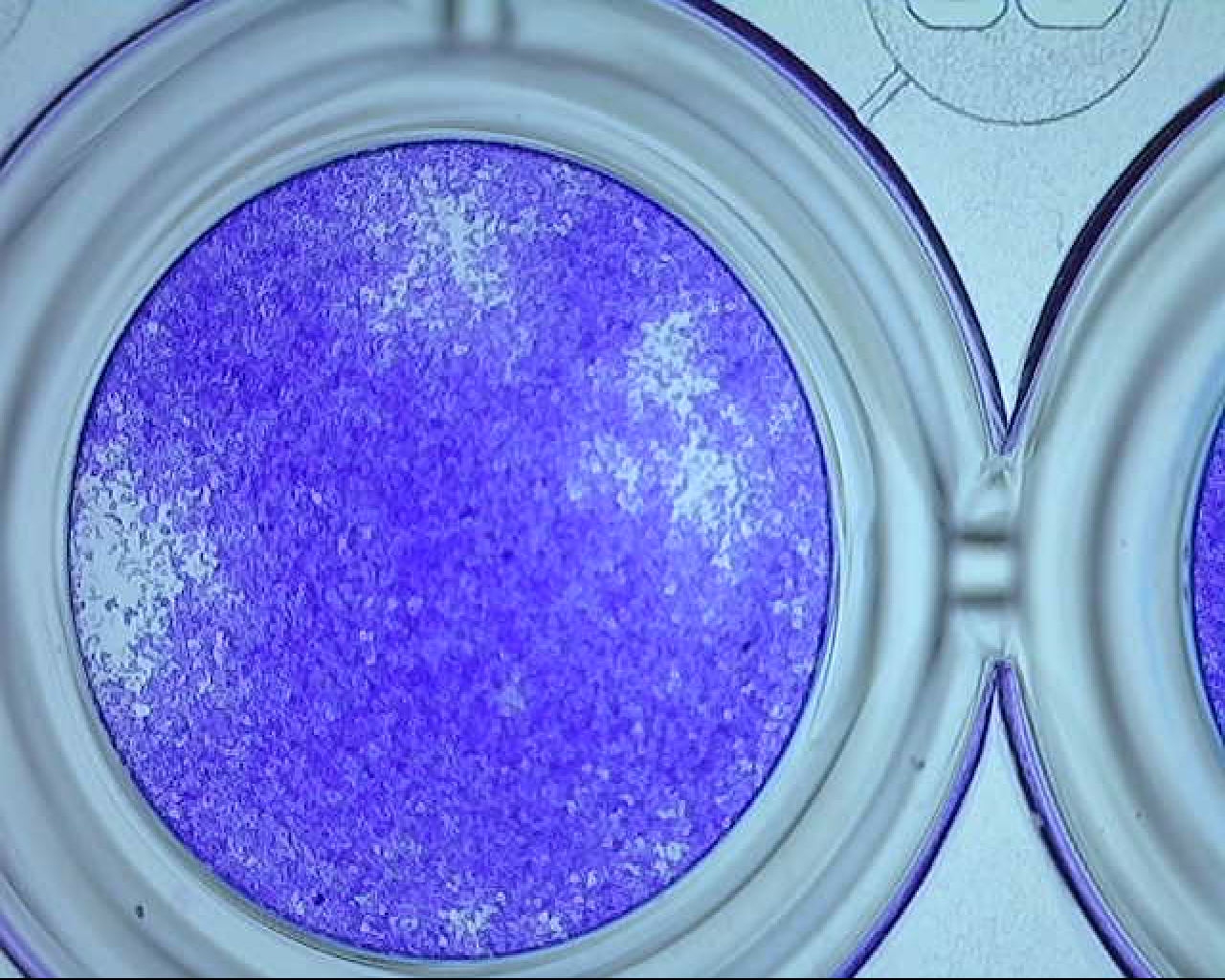
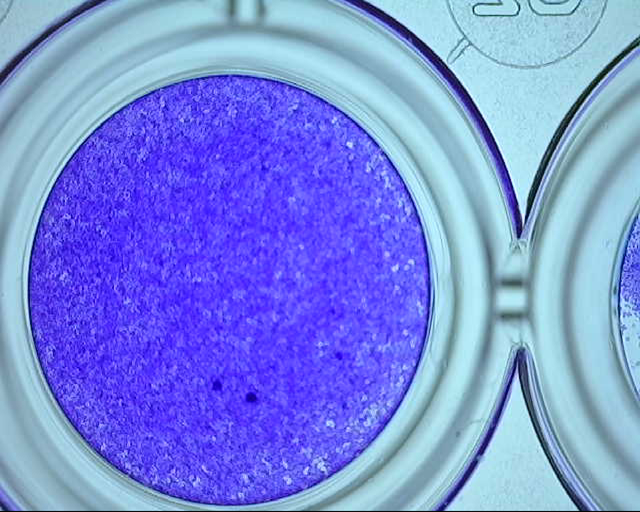
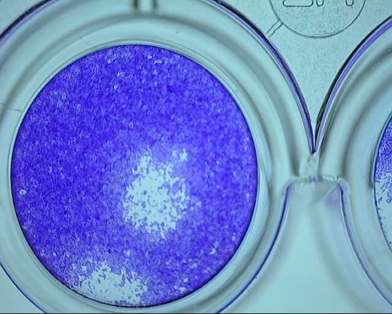
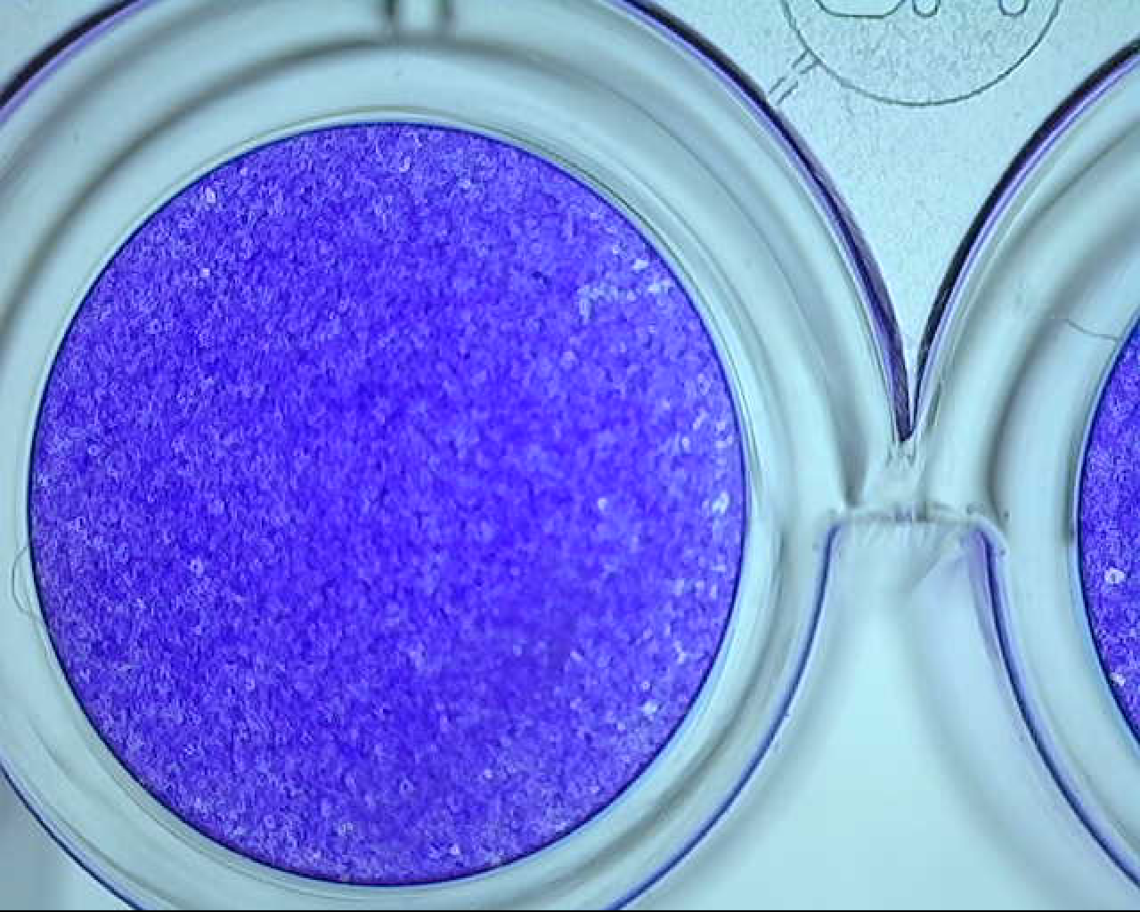
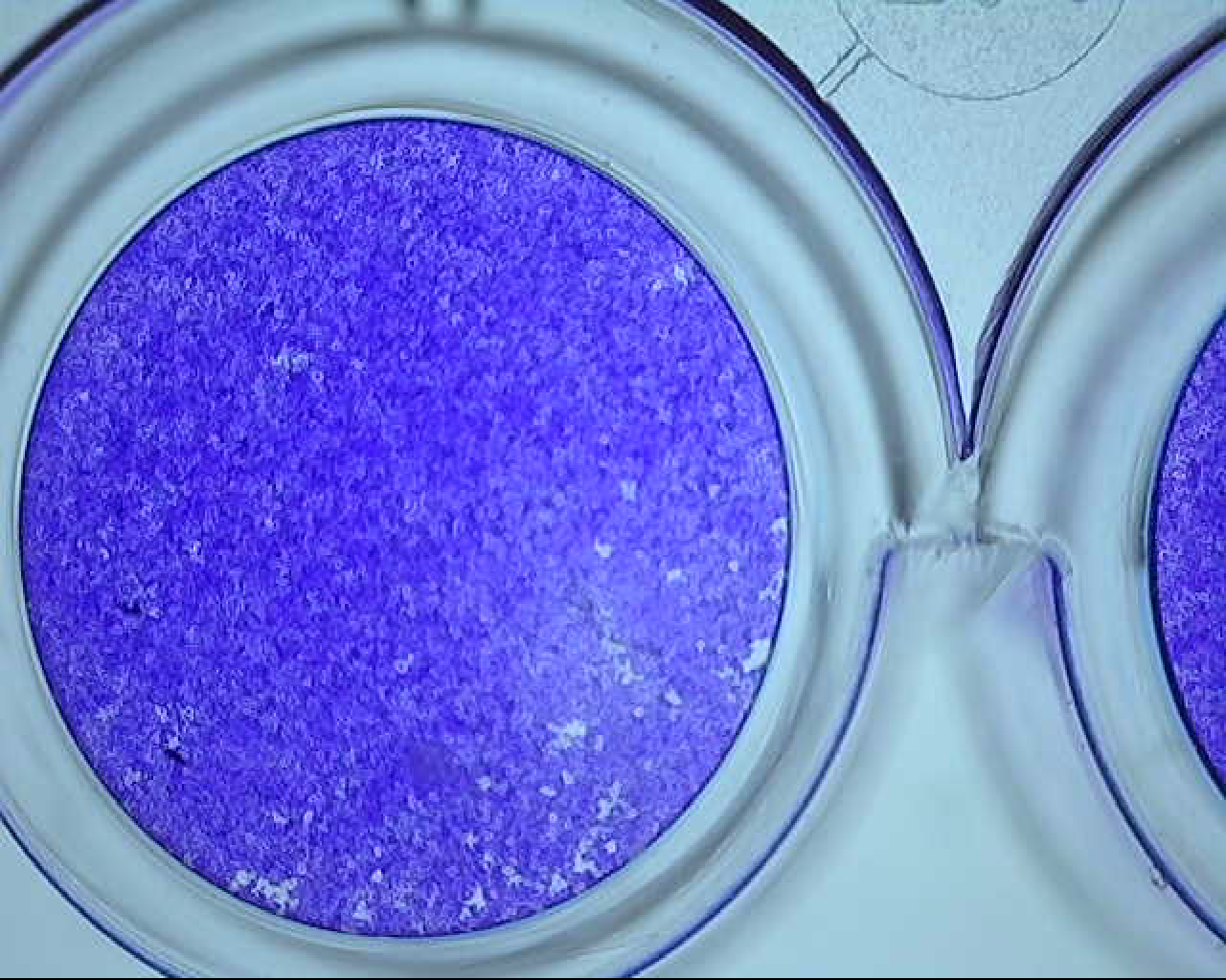
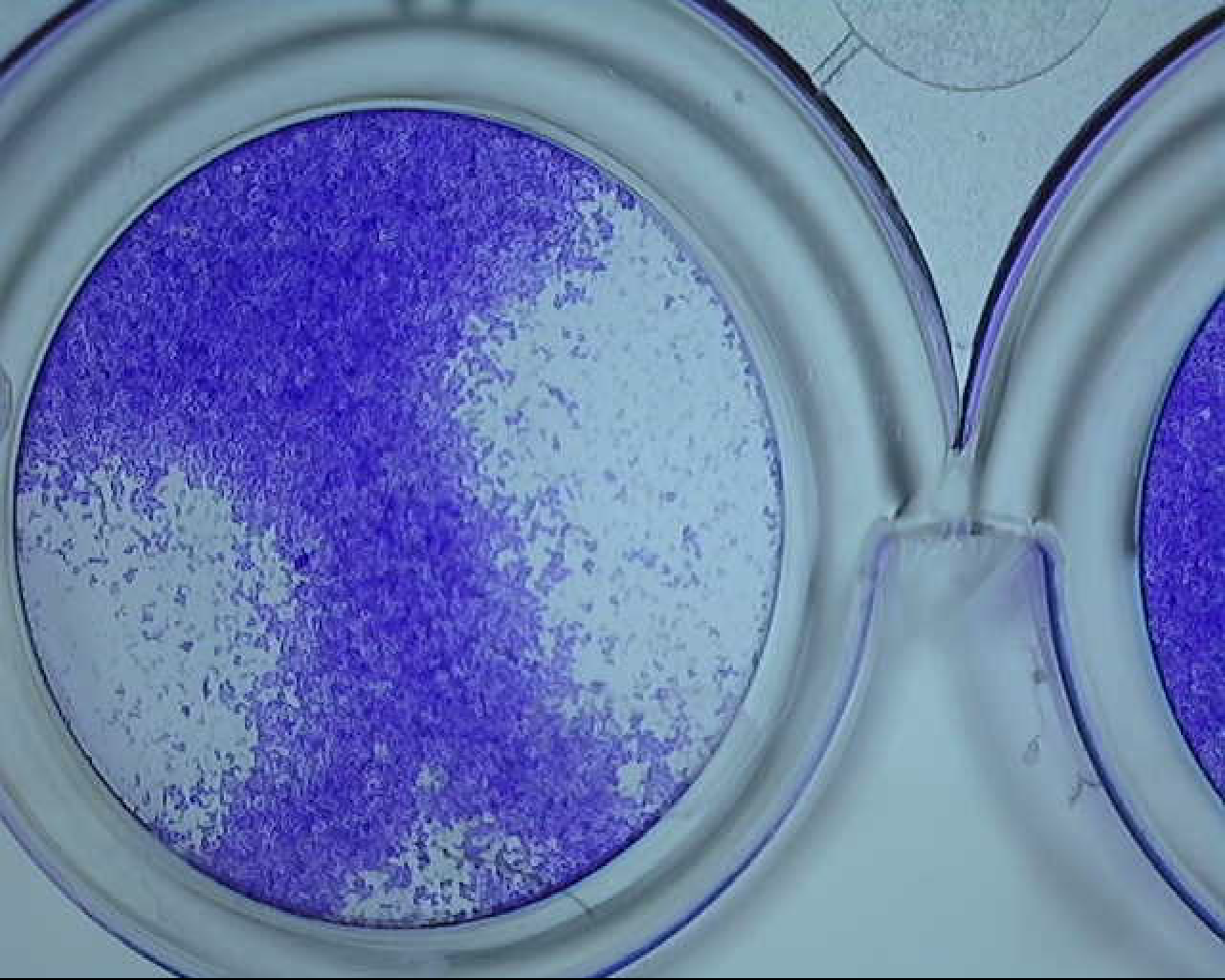
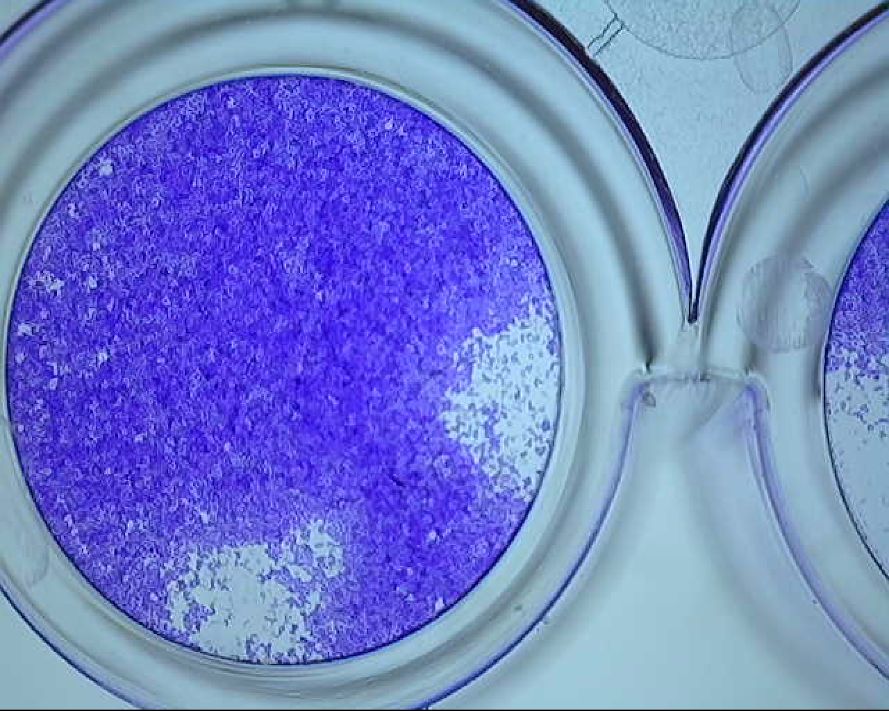
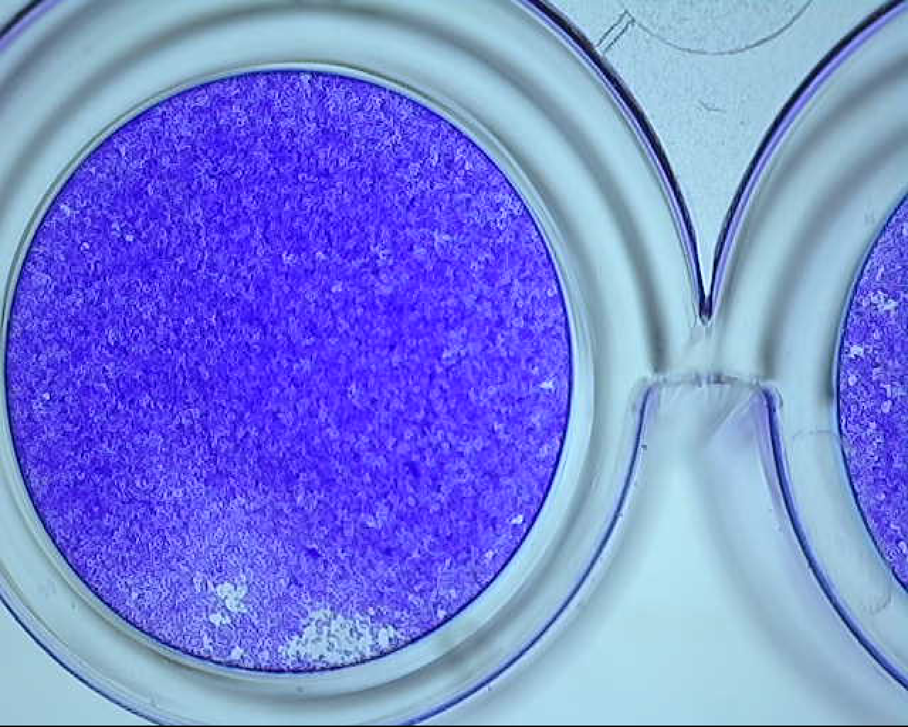
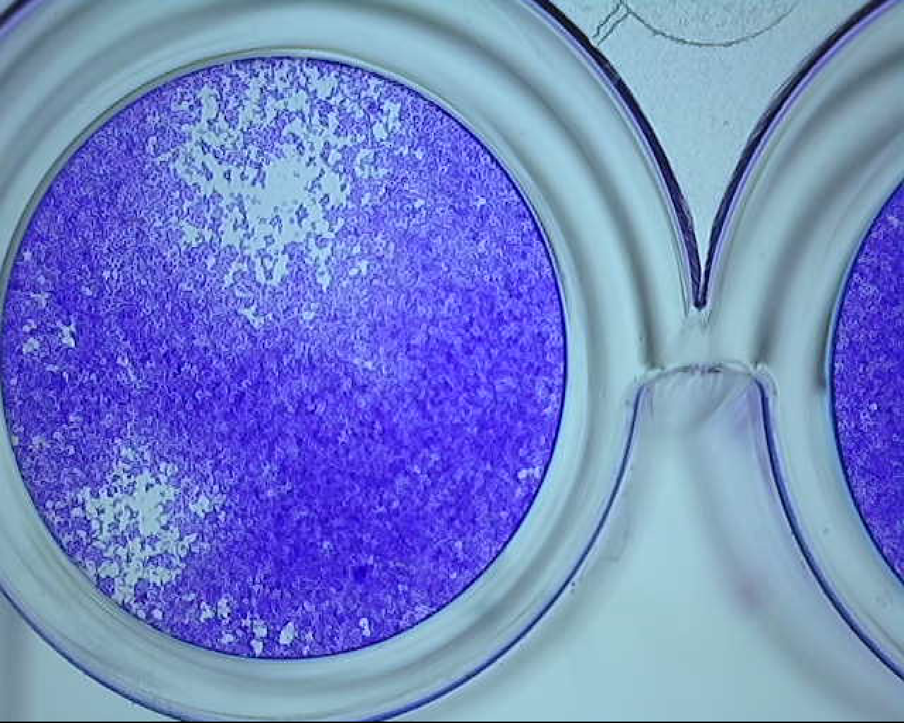
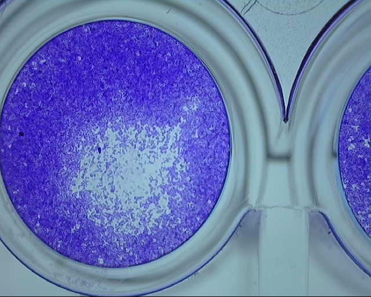
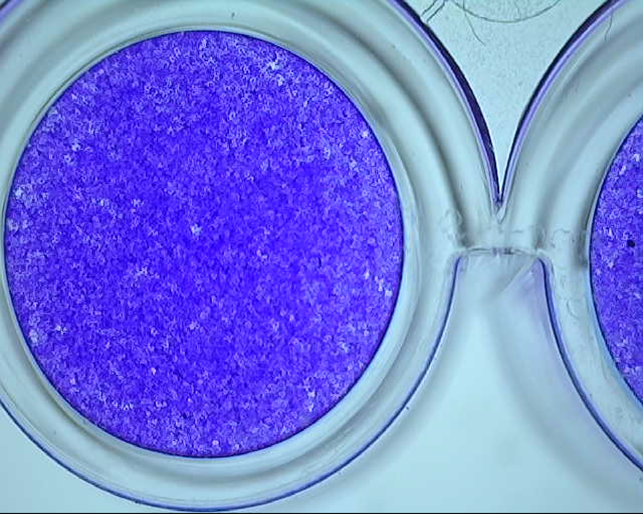
The viral plaque is surrounded by noninfected cells and is identified using a counterstain, typically a neutral red or crystal violet solution. The white areas indicate the virus plaques, which cause the solution around them to degrade. To count the viral plaques, three major steps are taken to process each image: locating the well position, filtering the color image for image enhancement, and counting the number of viral plaques with K-mean clustering.
The region of interest (ROI) is the focus region, which is important for counting viral plaques. The ROI is determined first, followed by the algorithms applied to the corrected location to prevent algorithm error. To locate the well position, a shape-based matching algorithm is employed to find the best matches of a shape model in an image (MVTec Software GmbH, 2021b). It does not use the gray values of pixels and their neighborhood as a template, but it defines the model by the shape of contours. In this case, the circular shape of the well is used as the template. Then, the algorithm finds the best-matched instance of the shape model. The position and rotation of the found instances of the model are returned in the pixel coordinates and angle, which are used to create the ROI image.
There are many techniques for filtering color images for image enhancement, including converting the RGB color space to HSV color space or binary image and applying a mean filter. Herein, the CIELAB color space is employed (MVTec Software GmbH, 2021a; Ly et al., 2020). It presents a quantitative relationship of color on three axes: L* represents the lightness, a* represents the red–green component of a color, and b* represents the yellow–blue component of a color. The CIELAB color space decouples the relationship between lightness and color of an image. Thus, the image brightness is less effective for image-processing. Only a* and b* are used to convert the image to a binary image. The a* and b* values of image pixels in ROI are used for clustering into the two groups, white and dark groups, by K-mean clustering, as shown in Fig. 3A. The yellow area represents the white group or white area, and the blue area represents the dark group or dark area. The red dot represents the centroid of each area. The result of the binary image is shown in Fig. 3B. After this process, a mean filtering process is applied to the binary image.
To count the number of viral plaques, a simple image threshold is employed for region selection. The suspected viral plaque regions are selected and analyzed. An example of suspect regions is shown in Fig. 4A. If the size, length, area, and roundness of a region are appropriated, the region is counted as the viral plaques. An example is shown in Fig. 4B. However, if the size and area of a region are too large because of their overlay, the K-mean clustering is employed in the region. To do that, the grid points are generated inside the large regions along the x–y coordinate, as shown in Fig. 4C. Then, K-mean clustering is employed to cluster the grid points. Moreover, to determine the optimal value of k or the appropriate cluster number, the Silhouette algorithm (Ogbuabor & Ugwoke, 2018) is implemented. The grid points are clustered into k clusters by K-mean clustering. Then, the average Silhouette coefficients for each k cluster are calculated. The Silhouette plot is shown in Fig. 4D. The maximum value of the average Silhouette coefficients is considered the optimal number of clusters. Finally, the number of viral plaques is the summation of the optimal number of clusters and the previous number of viral plaques (Fig. 4E).
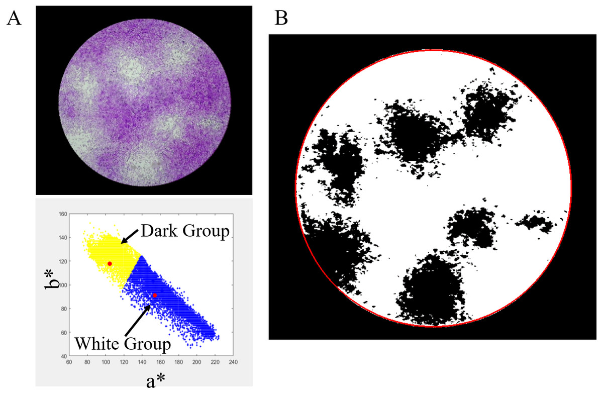
Figure 3: Converting RGB image to binary image.
(A) a* and b* values of image pixels. (B) Binary image by K-mean clustering.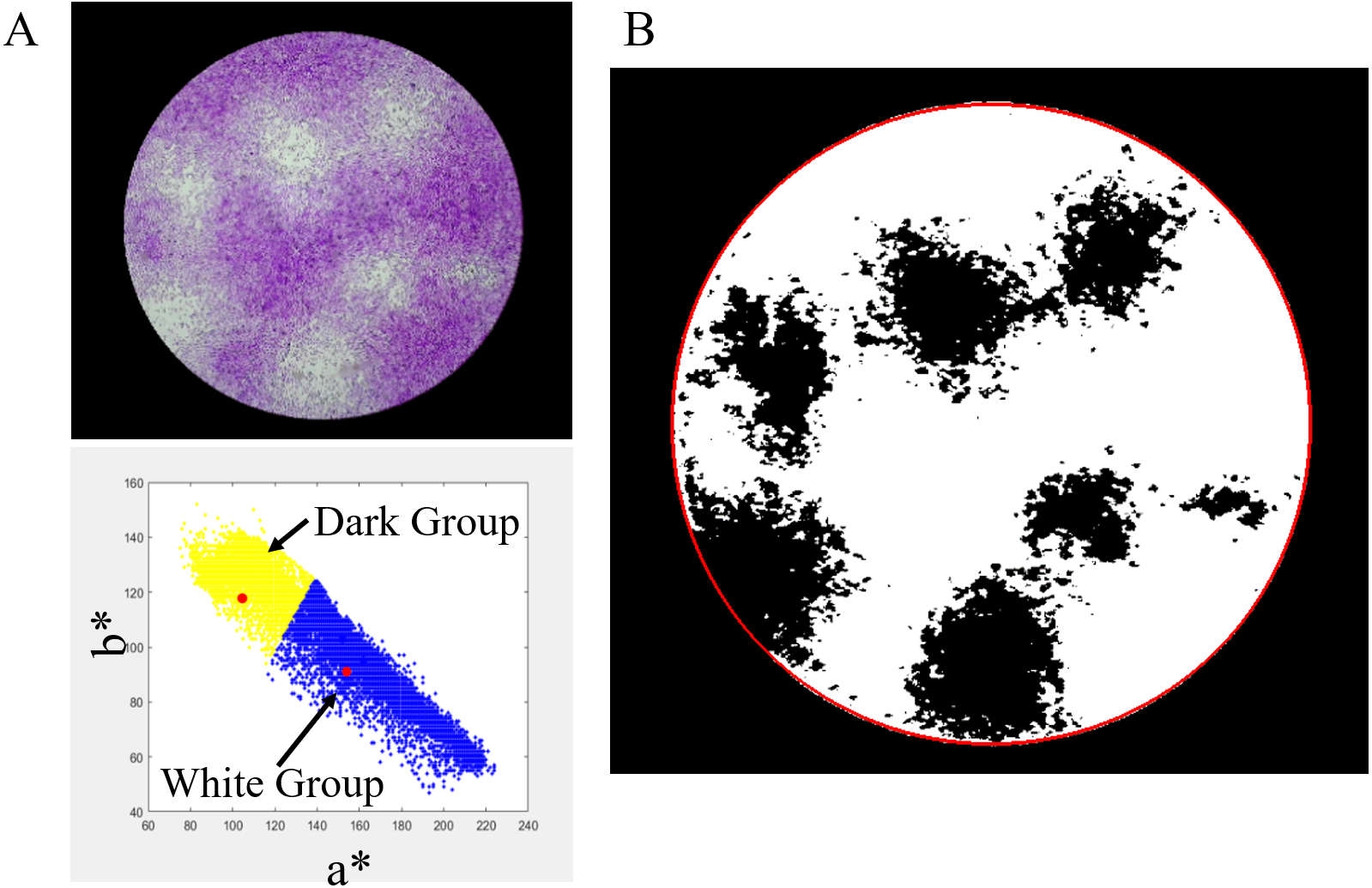
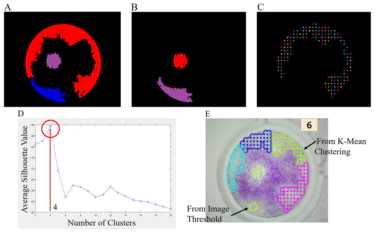
Figure 4: Viral plaque counting with K-mean clustering algorithm.
(A) Suspect viral plaque regions. (B) Appropriated region. (C) Grid points inside the larger region. (D) Silhouette plot. (E) Final result.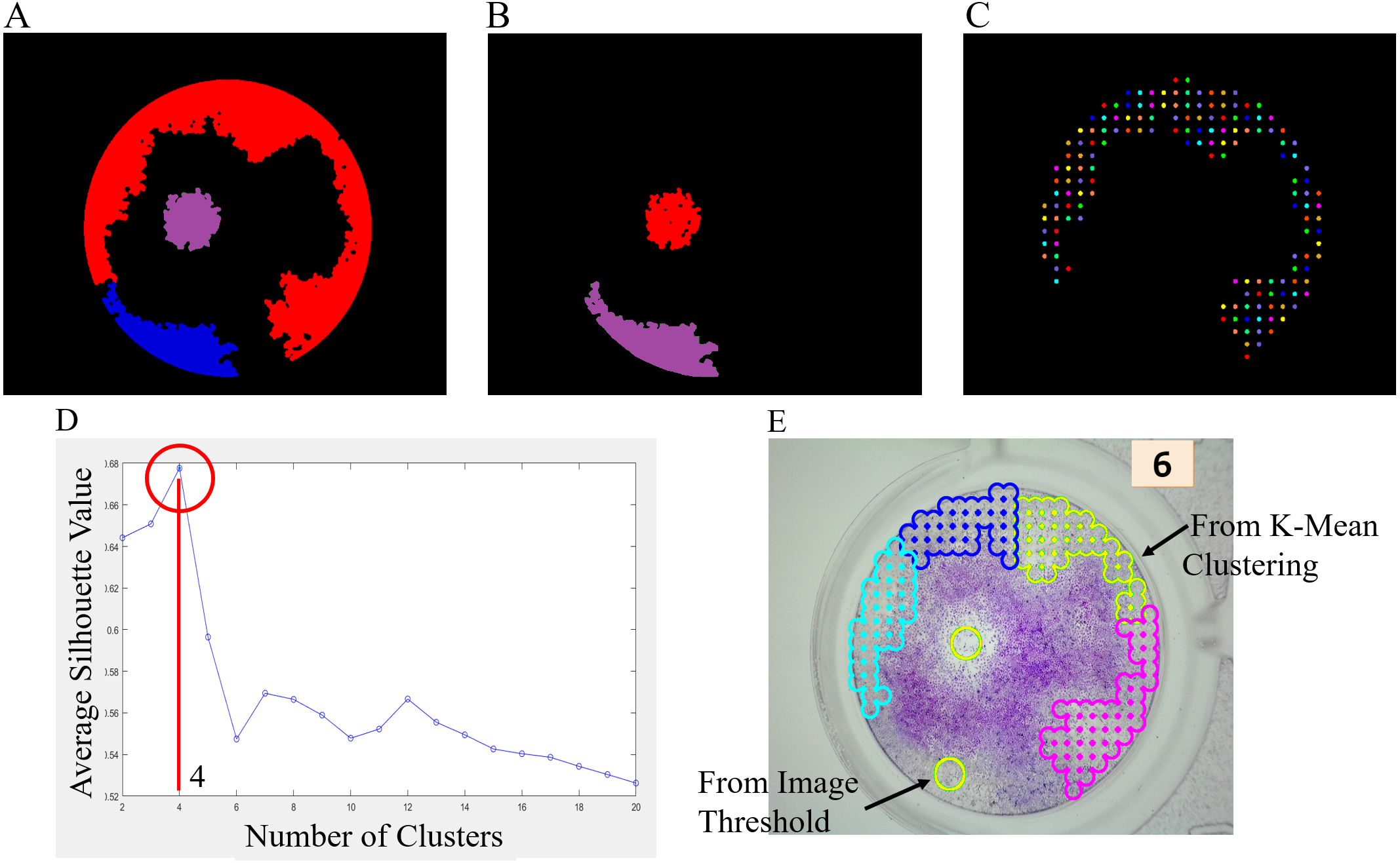
A flowchart of the ML-based software for image viral plaque counting is shown in Fig. 5, and an example of the machine counting results is shown in Fig. 6.
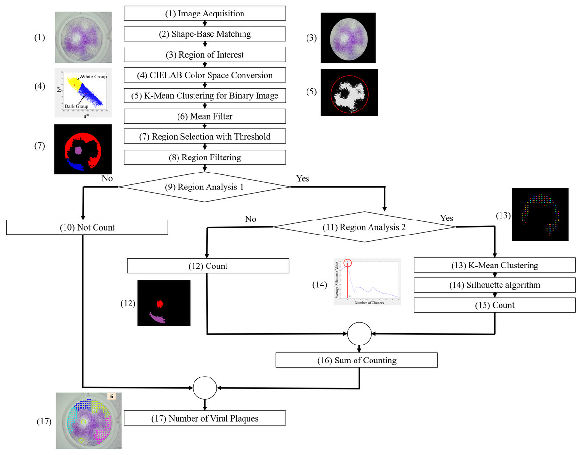
Figure 5: Machine learning (ML)-based software for image viral plaque counting.
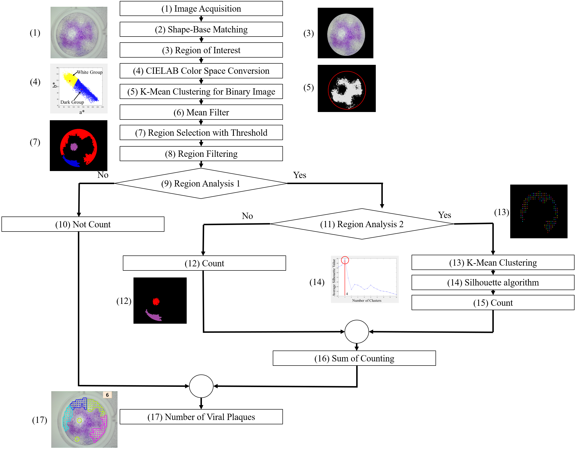
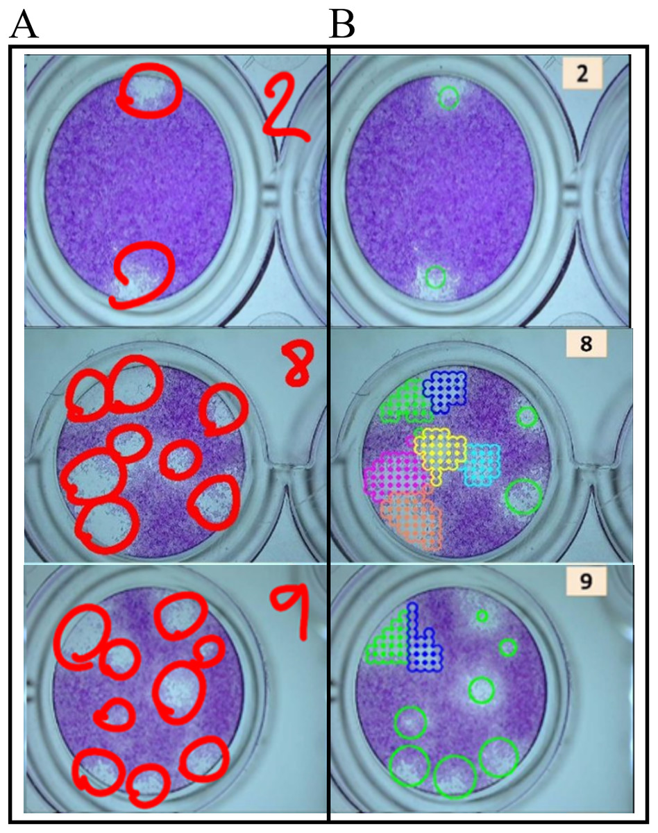
Figure 6: Example of machine counting.
(A) Counting results by an expert. (B) Counting by machine.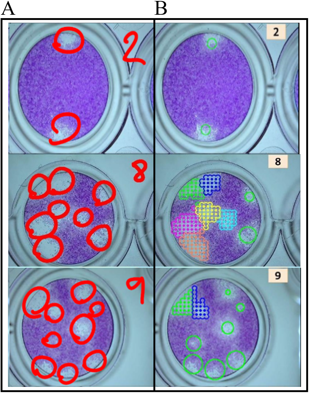
Viral plaque reading differences by humans
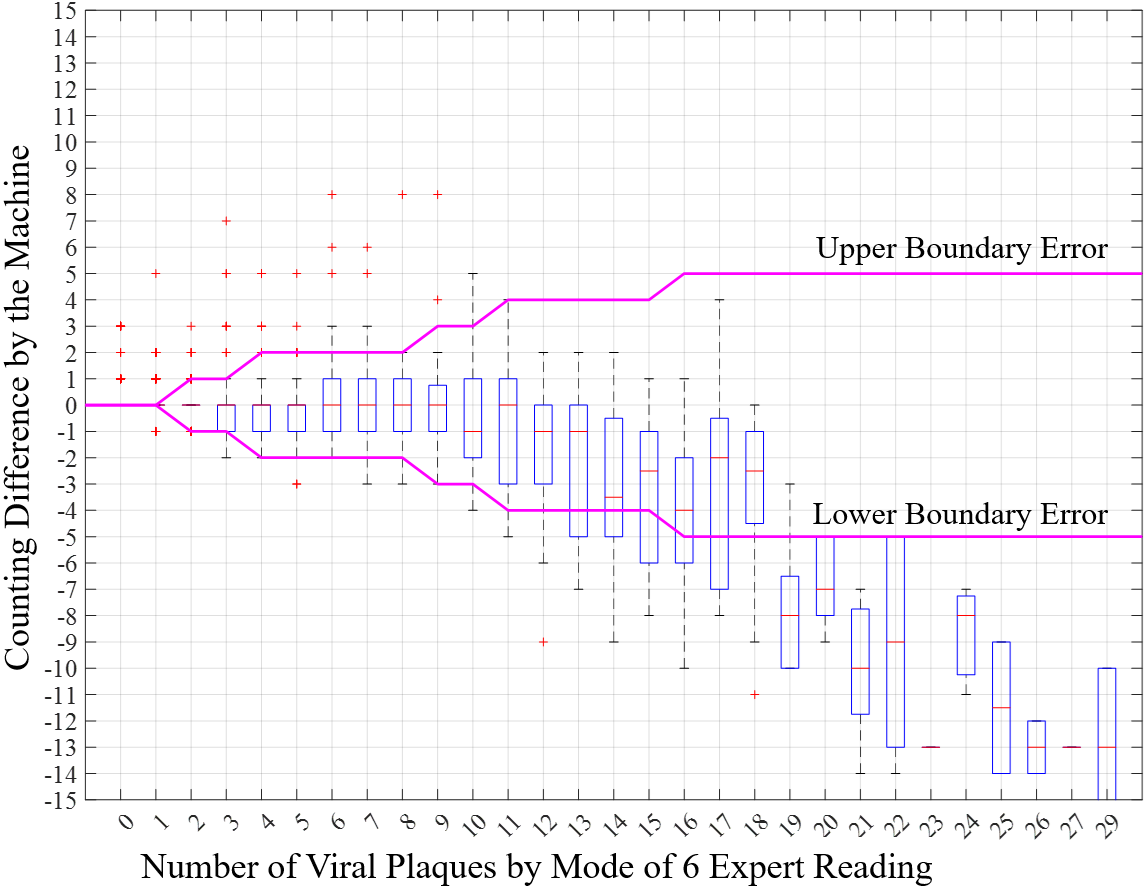
Plaque assays were created at the Medical Virology Research Center, Chulalongkorn University, Thailand. More than 25 96-well plates of dengue virus were used to evaluate differences in viral plaque readings. The number of viral plaques from 96-well plates was read by six experts, which included 1,777 wells that could be read by all experts. The remaining wells could not be read by experts, either because they were unclear or because no viral plaques were present; hence, they were not included in the evaluation. The number of viral plaques read by experts ranged between 0 and 31. To evaluate variations in expert readings, a boxplot of expert reading results for a given number of viral plaques is presented in Fig. 7. Since the actual number of viral plaques is unknown, the mode value of six expert readings was used as a reference in this case. Data that had no mode was not included in the evaluation. Figure 7A shows the distribution of readings by all experts for each number of viral plaques and Fig. 7B shows an example reading distribution by an expert for different numbers of viral plaques.
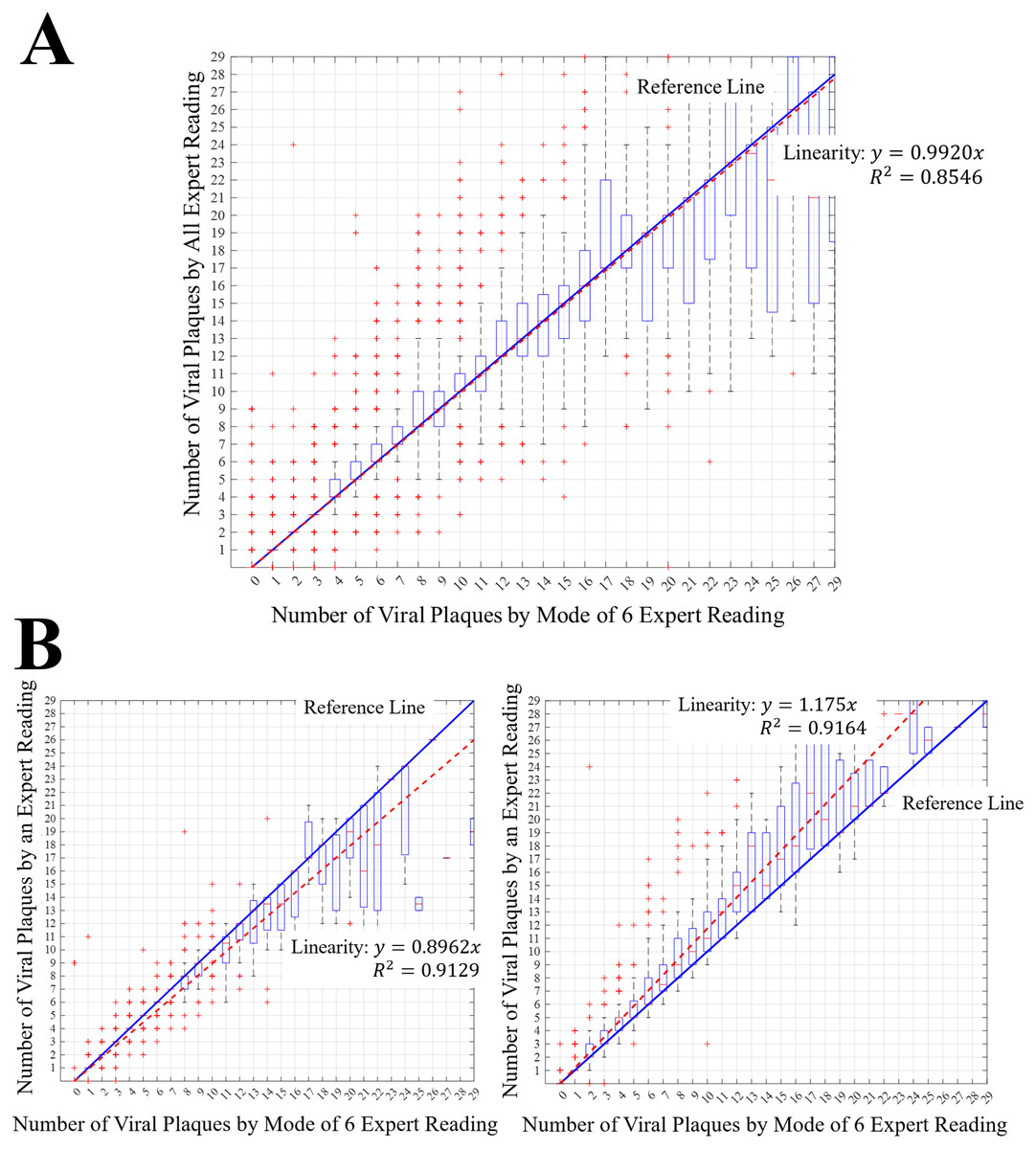
Figure 7: Expert reading distributions.
(A) Reading distribution of all experts for each number of viral plaques. (B) Reading distribution examples of an expert for each number of viral plaques. The red + marks represent the outliners of the measurement. The blue line having the slope of 1 represents the measurement reference values. The red dashed line represents the trend line of the measurement results of experts.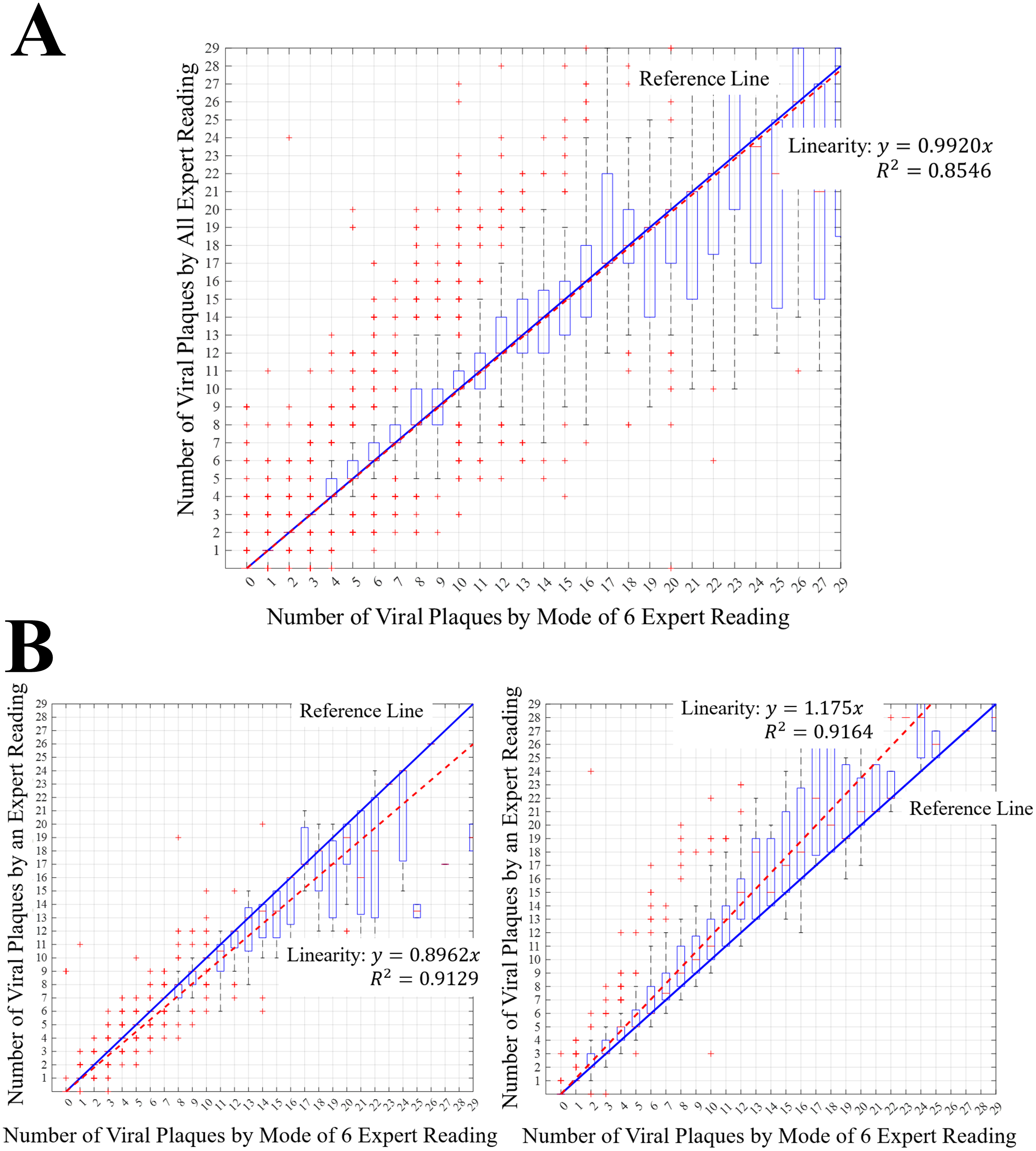
Figure 7 shows that the expert reading distributions in the range of 0–3 are small, but the distribution of expert readings increases when the number of viral plaques increased. When the number of viral plaques exceeds 12, the range of possible readings by an expert varies by more than a factor of 5.
To understand the variation in expert readings, a gage repeatability and reproducibility (R&R) analysis was employed (Automotive Industry Action Group, 2010; Burdick, Borror & Montgomer, 2005). A random sample of 300 wells (part) with and without viral plaques was used, in which the number of viral plaques varied from 0–25. Each well was subsequently read by six experts/operators. The results of the gage R&R were evaluated using a nested model (The MathWorks Inc, 2021) and analysis of the expert data was executed in MATLAB (The MathWorks Inc, 2021) using the MATLAB Toolbox to examine the results.
The gage R&R analysis was performed for various numbers of viral plaques in six ranges: 0–1, 2–3, 4–8, 9–10, 11–15, 16–25, and 0–25. The results are shown in Table 1.
| Reference number of viral plaques | ||||||||||||||
|---|---|---|---|---|---|---|---|---|---|---|---|---|---|---|
| 0–1 | 2–3 | 4–8 | 9–10 | 11–15 | >16 | All | ||||||||
| Var. | Sigma | Var. | Sigma | Var. | Sigma | Var. | Sigma | Var. | Sigma | Var. | Sigma | Var. | Sigma | |
| Gage R&R | 0.8847 | 0.9406 | 1.5433 | 1.2423 | 6.3720 | 2.5243 | 7.2413 | 2.6910 | 9.2160 | 3.0358 | 21.9960 | 4.6900 | 7.8756 | 2.8063 |
| Repeatability | 0.8510 | 0.9225 | 1.2298 | 1.1090 | 3.9490 | 1.9872 | 5.2781 | 2.2974 | 5.3403 | 2.3109 | 10.0464 | 3.1696 | 5.6792 | 2.3831 |
| Reproducibility | 0.0337 | 0.1835 | 0.3136 | 0.5600 | 2.4230 | 1.5566 | 1.9632 | 1.4011 | 3.8757 | 1.9687 | 11.9496 | 3.4568 | 2.1964 | 1.4820 |
| Operator | 0.0337 | 0.1835 | 0.3136 | 0.5600 | 2.4230 | 1.5566 | 1.9632 | 1.4011 | 3.8757 | 1.9687 | 11.9496 | 3.4568 | 2.1964 | 1.4820 |
| Part | 0.3568 | 0.5973 | 0.5092 | 0.7136 | 5.4656 | 2.3379 | 2.0874 | 1.4448 | 4.2479 | 2.0610 | 6.3211 | 2.5142 | 39.8431 | 6.3121 |
| Total | 1.2415 | 1.1142 | 2.0525 | 1.4327 | 11.8376 | 3.4406 | 9.3288 | 3.0543 | 13.4639 | 3.6693 | 28.3171 | 5.3214 | 47.7187 | 6.9079 |
Table 1 indicates that in the range of 0–1, the variation or sigma of expert readings according to the R&R process is 0.9406. The variation or sigma increases as the range of viral plaque numbers increases. The variation or sigma reaches as high as 4.6900 in the range of 16–25. For the overall range of 0–25, the variation or sigma is 2.8063. The reading distribution and reading variation values were used to design the experiment setup described in the following section.
Experiment
More than 25 96-well plates of dengue virus were used to evaluate the automated quantification machine. The 96-well plates were put in the machine, and their images were captured. Then, the images were screened for evaluation. There were 1,777 images qualified for evaluation. Next, the number of viral plaques in each image was manually determined by six experts from the research center and by the automated quantification machine software (note that 721 images showed 0 viral plaque). The number of viral plaques was evaluated based on the mode of expert readings and well as by the machine.
In the case of many viral plaques in an image, the image was ambiguous. For this reason, the number of viral plaques complicated efforts by the experts to read them. Therefore, an experimental counting criteria was defined based on the reading distribution in Fig. 7, the variation in expert readings in Table 1, and the criterion of the Medical Virology Research Center. If the difference between the number of viral plaques counted by the expert reading mode and the machine is within the maximum number of errors (Table 2), the number of viral plaques counted by the machine is correct. This counting criterion was employed in the evaluation, and the results are presented in the Results section.
The gage R&R analysis was employed to evaluate the repeatability and reproducibility of the machine (Automotive Industry Action Group, 2010; Burdick, Borror & Montgomer, 2005). For the analysis, 240 wells (part) with and without viral plaques were used. Due to the number of samples, the number of viral plaques of the 240 wells varied from 0 to 18. Then, each well was put into the machine to be captured the image and count the number of viral plaques. This procedure was repeated three times to represent three operators using the machine to count the number of viral plaques. Finally, each well has three measurement results from the machine. The gage R&R using the nested model is employed to evaluate the results (The MathWorks Inc, 2021).
MATLAB and MATLAB Toolbox were used to perform the analysis and the gage R&R analysis of the machine data.
Results
Distribution software counting for each number of viral plaques
The measurement of the number of viral plaques is depicted in Fig. 8. There are 1,777 measurements in the range of 0 to 29 viral plaques. For each number of viral plaques, the boxplot is used to show the mean and distribution of the measurement by the machine. The red + marks represent the outliners of the measurement, which includes less than 5% of the measurement. The boxplot shows that in the range of 0 to 9 viral plaques, the standard deviation (SD) of the measurement is less than 1, and the SD increases as the number of viral plaques increases.
| Reference number of viral plaques | Maximum number of errors |
|---|---|
| 0–1 | ±0 |
| 2–3 | ±1 |
| 4–8 | ±2 |
| 9–10 | ±3 |
| 11–15 | ±4 |
| >16 | ±5 |
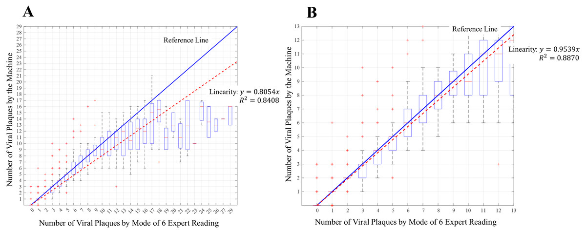
Figure 8: Distribution software counting for each number of viral plaques.
(A) Distribution of software counting for each number of viral plaques. (B) Distribution of software counting for the range [0–12] of number of viral plaques. The red + marks represent the outliners of the measurement. The blue line having the slope of 1 represents the measurement reference values. The red dashed line represents the trend line of the measurement results of the machine.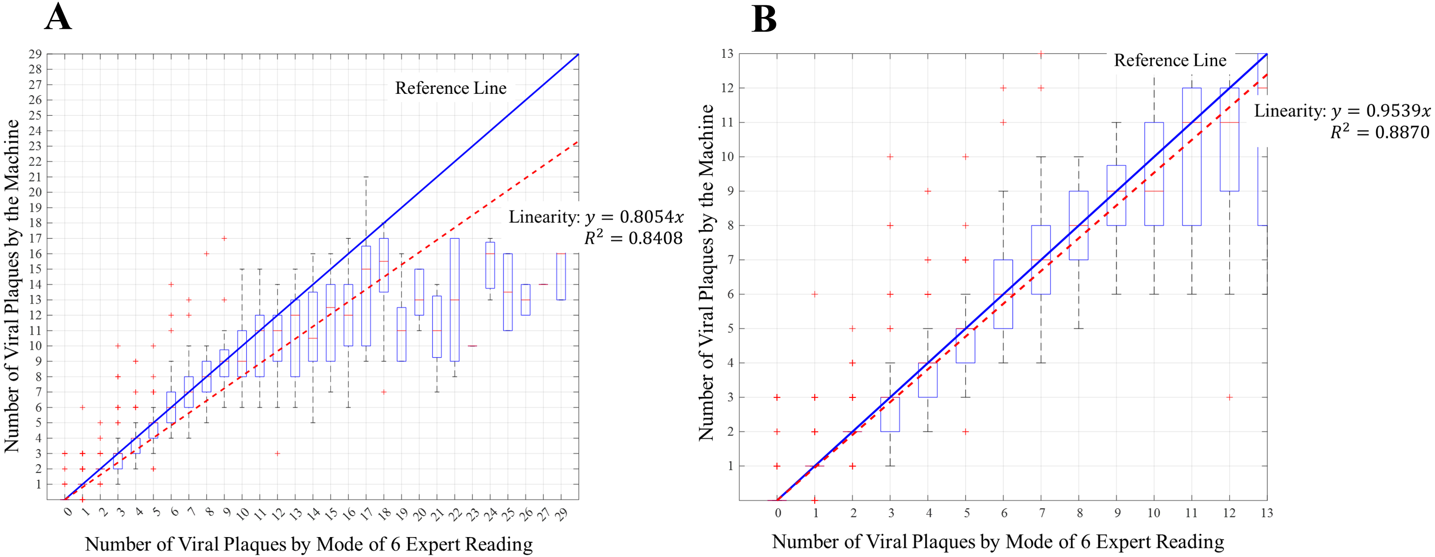
The blue line having the slope of 1 represents the measurement reference values. The red dashed line represents the trend line of the measurement results of the machine. The number of viral plaques obtained by the machine ranges from 0 to 29, as calculated form From Fig. 8A using Eq. (1). The goodness-of-fit equation generated an R2 of 0.8408. (1a)
Goodness-of-fit: (1b)
where y is the number of viral plaques by the machine, and x is the number of viral plaques by the expert. The values range from 0 to 29.
For Fig. 8B, the trendline of the measurement results of the machine shows the number of viral plagues ranging from 0 to 12, as calculated using Eq. (2). The goodness-of-fit equation generated an R2 of 0.8870. (2a)
Goodness-of-fit: (2b)
In the range of 0 to 29 viral plaques, the slope of the trend line of the machine is 0.8054, whereas, in the range of 0 to 12 viral plaques, the slope is 0.9539. For a number of viral plaques in the range of 0–12, the line has a slope close to 1 with R2 of 0.8870. Therefore, the counting results by the machine and experts correspond to the highest evaluation quality. Moreover, to evaluate the correlation between the counting by the expert and machine, Pearson’s coefficient method was used to measure the strength of the association between the machine and manual counting (Mukaka, 2012). The Pearson’s coefficient r of these variables is 0.9221 with a p-value of less than 0.0001. Since the p-value is less than 0.05, the variables reliably correlate.
Bland–Altman
To evaluate the performance of the machine, the Bland–Altman plot was used (Myles & Cui, 2007). The measurements from the expert and machine were considered. The difference in the measurement results from the expert and machine, error mean bias, and error SD were determined. The Bland–Altman plot is shown in Fig. 9. The results indicate that 95.01% of the measurement error is in the upper and lower boundaries (±2 SD). Therefore, the error from the machine is within the boundary limit. The machine effectively and efficiently quantified the number of viral plaques.
Performance of the machine
Counting viral plaques is ambiguous, even by an expert. Thus, counting criteria were defined, as shown in Table 2. If the error between the number of viral plaques counted by the expert reading mode and machine is within the maximum number of errors, as shown in Table 2, the number of viral plaques counted by the machine is correct.
The counting error between expert mode and the machine is presented using the boxplot (Fig. 10). The magenta line presents the maximum number of errors for each reference number of viral plaques. Figure 10 shows that in the range of 0–18 viral plaques, the mean measurements of the machine are within the boundary error, and the error is acceptable. For the range of 19–29 viral plaques, the error is large and out of the boundary. Consequently, when the number of viral plaques is larger, it is more difficult to measure the number of viral plaques. The accuracy of the reading from the large number is not significant to quantify viral infection or research. Moreover, only 55 of the 1,777 images are in the range of 19–29 viral plaques.
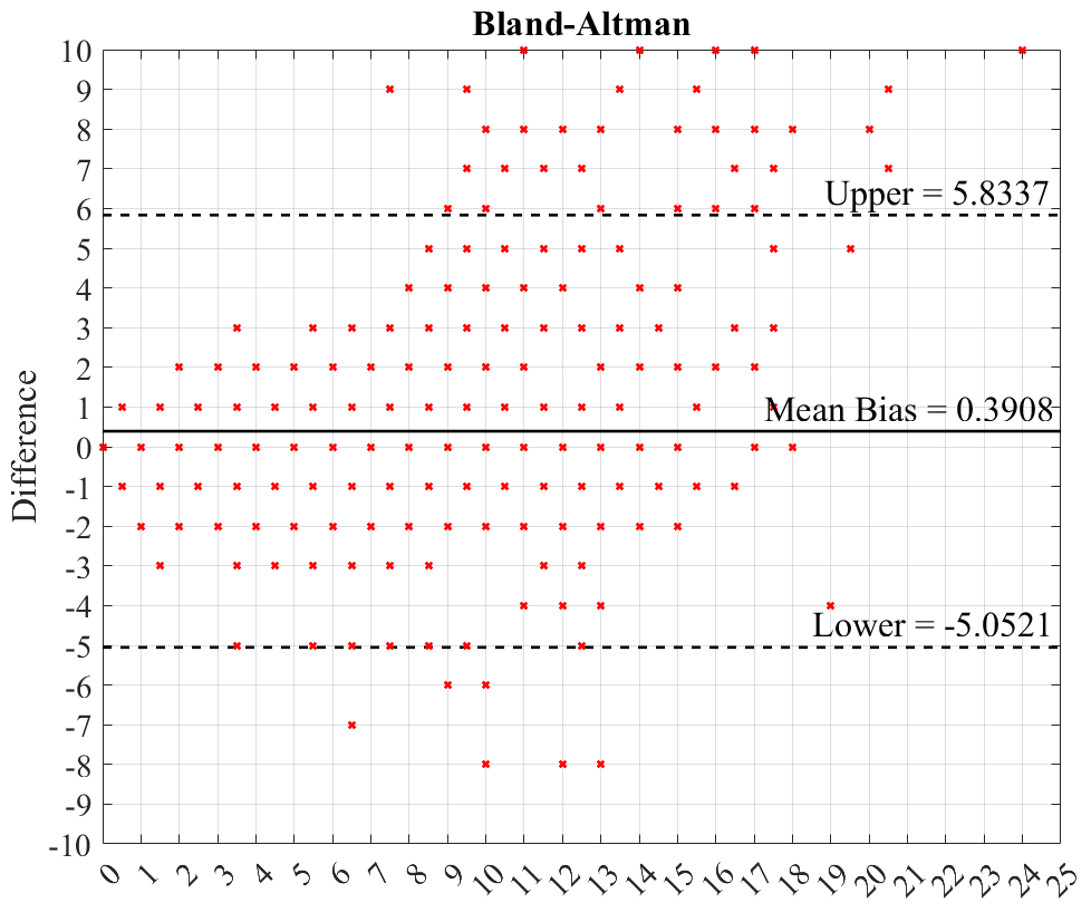
Figure 9: Bland–Altman plot of the machine measurement results.
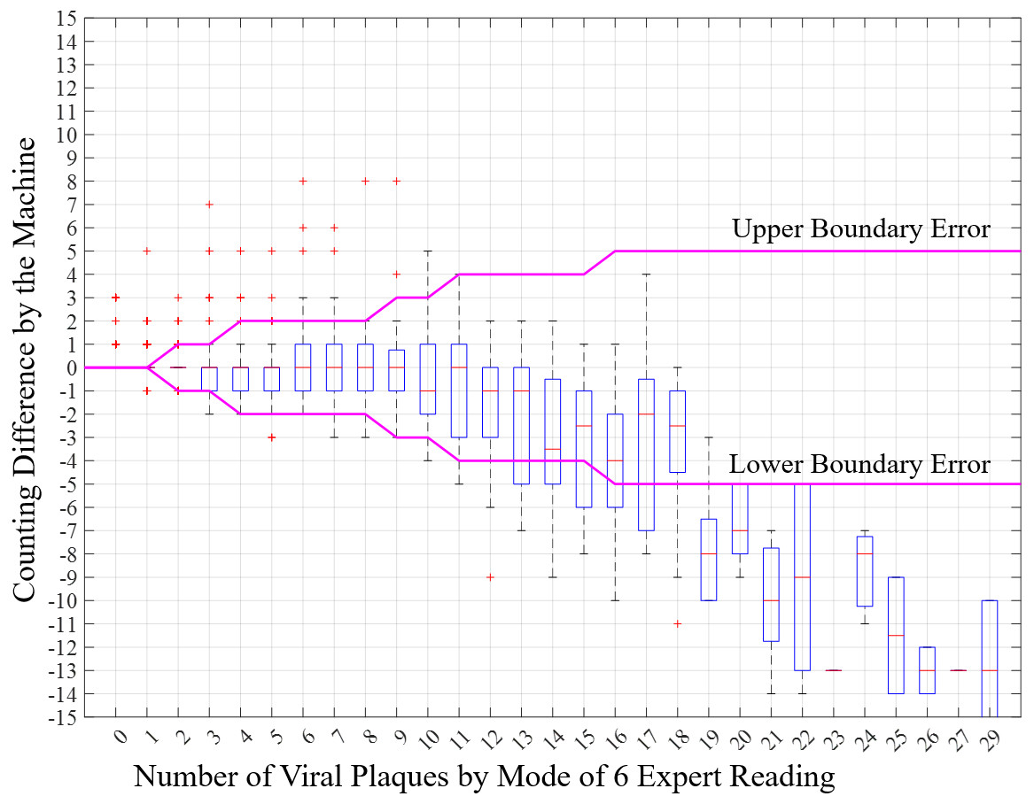
Figure 10: Distribution software error for each number of viral plaques.
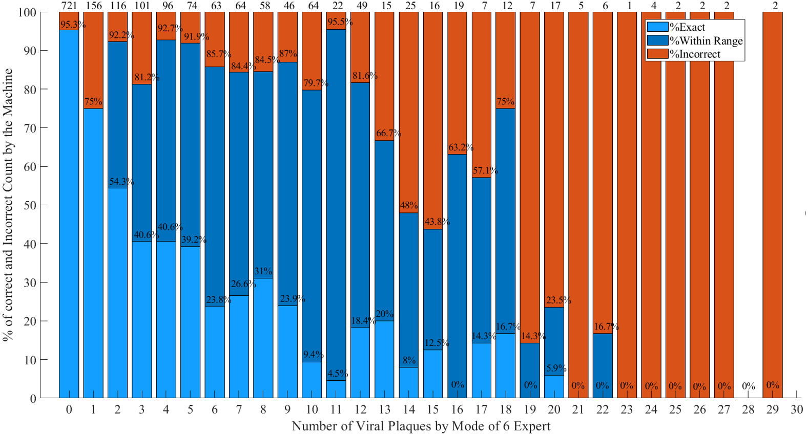
Based on the criteria in Table 2, the percentage of correct and incorrect measurements by the machine is shown in Fig. 11. The light blue bar represents the percentage of correct measurement which the machine measurement and expert reading mode are exactly the same. The dark blue bar represents the percentage of correct measurement which the machine measurement is within the defined range of expert reading mode and the red bar represents the percentage of incorrect measurement of the machine. The percentage of correct measurement is high when the number of viral plaques is low. In the range of 0–29 viral plaques, the percentage of correct measurement is more than 80%. In addition, the average correct measurement by the machine is 85.8%. This number is consisted of the percentages of exact correct and within the range are 60.0% and 25.8%, respectively.
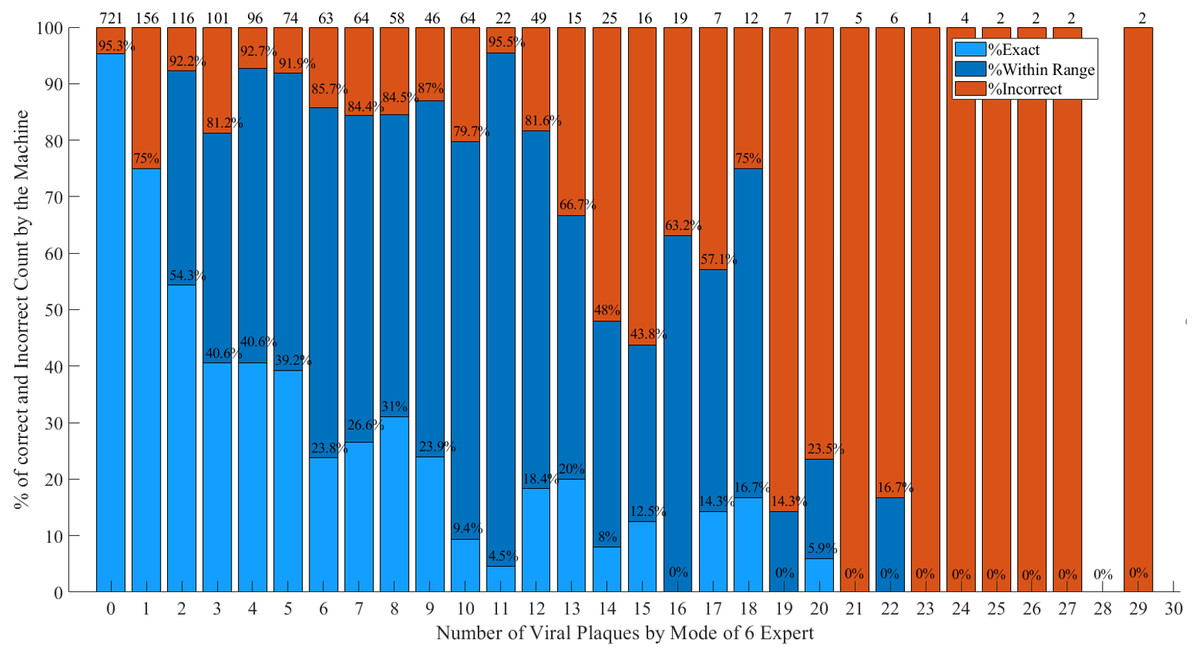
Figure 11: Percentage of correct measurement by the machine.
R&R of the Machine
The R&R of the machine was evaluated by gage R&R analysis according to Automotive Industry Action Group (2010) and Burdick, Borror & Montgomer (2005). The gage R&R is shown in Table 3. Previous authors (Automotive Industry Action Group, 2010; Burdick, Borror & Montgomer, 2005) suggest that the measurement system is acceptable if the number of distinct categories (NDC) is greater than or equal to 5. Moreover, for the percentage of gage R&R of total variations (PRR), the measurement system is capable if PRR is less than 10% and not capable if PRR is more than 30%. Otherwise, the measurement system is acceptable.
NDC of the machine is 6 and the PRR is 21.72%, which is between 10% and 30% criteria (Table 3). Due to the cost of the machine and previous results and evaluations, the R&R of the machine is acceptable, and the machine is capable of application.
Discussion
Counting the number of viral plaques is ambiguous, even for experts. Consequently, the Medical Virology Research Center defined experimental counting criteria for evaluating the machine output (Table 2) based on the distribution and variation of expert readings. If the number of viral plaques is small, the maximum number of errors is small, and as the number of viral plaques increases, the maximum number of errors increases. However, in the case of a large number of viral plaques, the reading accuracy is not sufficient for quantifying viral infection or in viral research.
| Source | Variance | %Variance | Sigma | 5.15 x sigma | % 5.15 x sigma |
|---|---|---|---|---|---|
| Gage R&R | 0.8861 | 4.7196 | 0.9413 | 4.8479 | 21.7246 |
| Repeatability | 0.0000 | 0.0000 | 0.0000 | 0.0000 | 0.0000 |
| Reproducibility | 0.8861 | 4.7196 | 0.9413 | 4.8479 | 21.7246 |
| Operator | 0.8861 | 4.7196 | 0.9413 | 4.8479 | 21.7246 |
| Part | 17.8891 | 95.2804 | 4.2296 | 21.7822 | 97.6117 |
| Total | 18.7752 | 100 | 4.3330 | 22.3151 |
Notes:
Number of distinct categories (NDC): 6.
% of Gage R&R of total variations (PRR): 21.72.
The last column of the above table does not to necessarily sum to 100%.
The automated quantification machine was evaluated using 96-well plates of dengue virus. According to the analysis, the measurement results obtained using the machine correlate well with the manual counting results. For 0–29 viral plaques, the trend line of the result of the machine has a slope of 0.8054 with R2 of 0.8408, and in the range of 0–12 viral plaques, the slope is 0.9539 with R2 of 0.8870. The correlation in the range of 0–12 viral plaques is better than that in the range of 0–29 viral plaques.
The Pearson’s coefficient r of the data is 0.9221 with a p-value of less than 0.0001. This shows that the machine counting results correlate with the manual counting results. Further, the Bland–Altman plot shows that more than 95% of the measurement errors are in the upper and lower boundaries (±2 SD). Thus, the manual and machine counting results are consistent.
As shown in Fig. 8B, for 0–12 viral plaques, the boxplot is close to the reference line, indicating the manual and machine counting results are in good agreement. However, for 13–29 viral plaques, the boxplot mean is below the reference line, indicating that the measurement results of the machine are less than the manual measurement results. This information can be used to improve the algorithm for measurement in the range of 13–29 viral plaques in future studies.
The large error in the results of the machine in the range of 13–29 viral plaques could be attributed to the criteria of the Silhouette algorithm. The Silhouette algorithm uses only the location information of the grid points to calculate the Silhouette score for selecting the suitable number of clusters. To improve the algorithm, other criteria, such as the number of grid points and areas, can be included in the algorithm to calculate the new Silhouette score.
Base on the gage R&R analysis, the major variations in PRR results from reproducibility, which occurs when the user puts the sample to the machine and measures the number of viral plaques. If the brightness of the environment light is changed, the image color may be changed, which affects the algorithm. This may be overcome by creating a cover for the machine to reduce the effect of environmental light. The repeatability of the machine is 0 since the counting algorithm has no variation.
According to the performance analysis, the average correct measurement of the machine is 85.8% in the range of 0–29 viral plaques. However, most of the errors occur when the number of viral plaques is high. If only small and medium numbers of viral plaques are evaluated, the average correct measurement of the machine would be more than 85.8%.
The plaque sizes varied by various conditions such as pH of the buffers, concentrations of the semisolid, or under antiviral treatment. Moreover, previous reports have optimized the plaque readings in 24- and 96-well plates in antiviral drug discovery (Boonyasuppayakorn et al., 2016; Katzelnick et al., 2018; Yin et al., 2019). In order to cover this issue, our developed software provides the manually adjustable plaque sizes customized by users. The user can config the parameters the range of plaque sizes, save, and use them for the specific scenario.
Even though there are automated imaging-based counters for plaque assay, the current commercial versions have multiple challenges, especially their complexity and cost. They may unsuitable for personal use in the laboratory. Thus, for situations of limited resources, the developed machine may be more suitable for a personal laboratory. Additionally, the developed machine can be applied to Elispot counting (Kukiattikoon et al., 2021).
Conclusions
The developed automated quantification machine with ML-based software effectively quantified the number of viral plaques in a 96-well plate in a simple process and at a low cost. The automated quantification machine was evaluated using 96-well plates of dengue virus. The performance analysis showed that the machine measurement results correlate well with manual counting results, and the average correct measurement by the machine is 85.8%. The machine meets the requirements of reducing workload and performing virus plaque assay reading in the laboratory.
Supplemental Information
The example results from an expert and the algorithm on plate 1
The example results from an expert and the algorithm on plate 2
The example results from an expert and the algorithm on plate 3
The example results from an expert and the algorithm on plate 4
The example results from an expert and the algorithm on plate 5
The example results from an expert and the algorithm on plate 6
The example results from an expert and the algorithm on plate 7
The example results from an expert and the algorithm on plate 8
The example results from an expert and the algorithm on plate 9
The example results from an expert and the algorithm on plate 10
The example results from an expert and the algorithm on plate 11
The example results from an expert and the algorithm on plate 12
The example results from an expert and the algorithm on plate 13
The example results from an expert and the algorithm on plate 14
The example results from an expert and the algorithm on plate 15
The example results from an expert and the algorithm on plate 16
The example results from an expert and the algorithm on plate 17
The example results from an expert and the algorithm on plate 18
The example results from an expert and the algorithm on plate 19
The example results from an expert and the algorithm on plate 20
The example results from an expert and the algorithm on plate 21
The example results from an expert and the algorithm on plate 22
The example results from an expert and the algorithm on plate 23
The example results from an expert and the algorithm on plate 24
The example results from an expert and the algorithm on plate 25
The example results from an expert and the algorithm on plate 26
The example results from an expert and the algorithm on plate 27
MVtec Halcon Code
1. Main.hdev: Main file to run the code
2. count_plaque.hdvp: Code script
3. kmeancluster.hdvp: Code script
4. Master.tif: template image for Main.hdev
5. license_eval_halcon_steady_2021_10.dat: license for Halcon program