
Comparing supervised and unsupervised approaches to multimodal emotion recognition
- Published
- Accepted
- Received
- Academic Editor
- Chintan Amrit
- Subject Areas
- Computer Vision, Data Mining and Machine Learning, Multimedia, Natural Language and Speech, Social Computing
- Keywords
- Affective computing, Facial expression, Multimodal emotion recognition, Supervised and unsupervised learning, Vocal expression
- Copyright
- © 2021 Fernández Carbonell et al.
- Licence
- This is an open access article distributed under the terms of the Creative Commons Attribution License, which permits using, remixing, and building upon the work non-commercially, as long as it is properly attributed. For attribution, the original author(s), title, publication source (PeerJ Computer Science) and either DOI or URL of the article must be cited.
- Cite this article
- 2021. Comparing supervised and unsupervised approaches to multimodal emotion recognition. PeerJ Computer Science 7:e804 https://doi.org/10.7717/peerj-cs.804
Abstract
We investigated emotion classification from brief video recordings from the GEMEP database wherein actors portrayed 18 emotions. Vocal features consisted of acoustic parameters related to frequency, intensity, spectral distribution, and durations. Facial features consisted of facial action units. We first performed a series of person-independent supervised classification experiments. Best performance (AUC = 0.88) was obtained by merging the output from the best unimodal vocal (Elastic Net, AUC = 0.82) and facial (Random Forest, AUC = 0.80) classifiers using a late fusion approach and the product rule method. All 18 emotions were recognized with above-chance recall, although recognition rates varied widely across emotions (e.g., high for amusement, anger, and disgust; and low for shame). Multimodal feature patterns for each emotion are described in terms of the vocal and facial features that contributed most to classifier performance. Next, a series of exploratory unsupervised classification experiments were performed to gain more insight into how emotion expressions are organized. Solutions from traditional clustering techniques were interpreted using decision trees in order to explore which features underlie clustering. Another approach utilized various dimensionality reduction techniques paired with inspection of data visualizations. Unsupervised methods did not cluster stimuli in terms of emotion categories, but several explanatory patterns were observed. Some could be interpreted in terms of valence and arousal, but actor and gender specific aspects also contributed to clustering. Identifying explanatory patterns holds great potential as a meta-heuristic when unsupervised methods are used in complex classification tasks.
Introduction
When people interact, they do not only use words to convey affective information, but also often express emotions through nonverbal channels. Main sources of nonverbal communication include facial expressions, bodily gestures, and tone of voice. Accurate recognition of others’ emotions is important for social interactions (e.g., for avoiding conflict and for providing support; Ekman, 2003; Russell, Bachorowski & Fernandez-Dols, 2003). Knowledge about how emotions are expressed nonverbally thus has applications in many fields, ranging from psychotherapy (e.g., Hofmann, 2016) to human-computer interaction (e.g., Jeon, 2017). Notably, research on the production and perception of emotional expressions has also been a main source of data for theories of emotion (e.g., Scherer, 2009). We employ machine learning methods to classify dynamic multimodal emotion expressions based on vocal and facial features and describe the most important features associated with a range of positive and negative emotions. We also compare traditional supervised methods with solutions obtained with unsupervised methods in order to gain new insights into how emotion expressions may be organized.
Meta-analyses of emotion perception studies suggest that human judges are able to accurately infer emotions from nonverbal vocal and facial behavior, also in cross-cultural settings (e.g., Elfenbein & Ambady, 2002; Laukka & Elfenbein, 2021). However, it has proved more difficult to define the physical features reliably associated with specific emotions. Juslin & Laukka (2003) proposed that nonverbal communication of emotion through the voice is based on a number of probabilistic and partly redundant acoustic cues. Probabilistic cues are not perfect indicators of the expressed emotion because they are not always associated with that emotion and can also be used in the same way to express different emotions. For example, high mean fundamental frequency (F0) can be associated with both happiness and fear. Several partly redundant cues can, in turn, be associated with the same emotion. For example, anger can be associated with high levels of both voice intensity and high-frequency energy. Barrett et al. (2019) similarly noted that facial cues (e.g., smiles) are only probabilistically associated with any one emotion (e.g., happiness), and that similar configurations of facial movements can be associated with more than one emotion.
The combination of probabilistic and partly redundant cues entails that there may be several cue combinations that are associated with the same emotion, which leads to a robust and flexible system of communication (Juslin & Laukka, 2003). For example, Srinivasan & Martinez (2021) recently reported that several different facial configurations were used to communicate the same emotion in naturalistic settings (e.g., they reported 17 different configurations for happiness). Machine learning methods are increasingly used to detect patterns in this type of high-dimensional probabilistic data. Recent years have seen much activity in the field of machine-based classification of emotions from facial (e.g., Li & Deng, 2020) and vocal (e.g., Schuller, 2018) expressions. Classifiers often perform on par with human judges, although performance also varies across emotions and databases (Krumhuber et al., 2021b). The majority of classification studies have been performed on unimodal stimuli (either vocal or facial), but combining features from several modalities has been shown to increase classification accuracy (see D’Mello & Kory, 2015, for a meta-analysis). The number of multimodal classification studies is steadily increasing (Poria et al., 2017), and recent studies explore a wide variety of approaches (e.g., Bhattacharya, Gupta & Yang, 2021; Lingenfelser et al., 2018; Mai et al., 2020; Siriwardhana et al., 2020; Tzirakis et al., 2017; Wang, Wang & Huang, 2020).
In the current study, we first compare how unimodal and multimodal classifiers perform in the classification of 18 different emotions from brief video recordings. Recordings are taken from the Geneva Multimodal Emotion Portrayal (GEMEP) corpus (Bänziger, Mortillaro & Scherer, 2012), which contains dynamic audio-video emotion expressions portrayed by professional actors. This approach extends most previous classification studies which have focused on a much smaller number of emotions, but is in line with recent perception studies which suggest that human judges can perceive a wide variety of emotions (e.g., Cordaro et al., 2018). Different actors are used for training and testing in all classification experiments, to avoid person bias. We also contribute by providing details of which features are important for classification of which emotions–something only rarely done in machine classification (see Krumhuber et al., 2021b, for a recent example).
We analyze the physical properties of vocal expressions by extracting the features included in the Geneva Minimal Acoustic Parameter Set (GeMAPS; Eyben et al., 2016). This parameter set is commonly used in affective computing and provides features related to the frequency, intensity, spectral energy, and temporal characteristics of the voice. Facial Action Units (AUs) (Ekman & Friesen, 1978)—which is one of the most comprehensive and objective ways to describe facial expressions (Martinez et al., 2019)—are also extracted. This selection of vocal and facial features allows for comparisons with the previous literature on emotion expression. Finally, we compare the results from the supervised classification experiments with results from unsupervised classification. Unsupervised methods may reveal new information about how emotion expressions are organized, because they are not restricted to any pre-defined emotion categories (e.g., Azari et al., 2020).
Methods
Data, code, and additional computational information are openly available on GitHub (see Data Availability statement).
Emotion expressions
The emotion expressions used in this study were taken from the GEMEP database (Bänziger, Mortillaro & Scherer, 2012) and consist of 1,260 video files in which 10 professional actors, coached by a professional director, convey 18 affective states. They do this by uttering two different pseudolinguistic phoneme sequences, or a sustained vowel ‘aaa’. The emotions portrayed in this dataset are: admiration, amusement, anger, anxiety/worry, contempt, despair, disgust, interest, irritation, joy/elation, panic fear, sensual pleasure, pride, relief, sadness, shame, surprise, and tenderness. The number of files per emotion and actor can be seen in Fig. S1. The GEMEP dataset was chosen for its high naturalness ratings and wide range of included emotions. It is widely used in classification studies (e.g., Schuller et al., 2019; Valstar et al., 2012), although few previous studies have included all 18 emotions.
Feature extraction and pre-processing
Audio features were obtained using openSMILE 2.3.0 (Eyben et al., 2013), an open-source toolkit that allows for the extraction of a wide variety of parameter sets. In this study, two different versions of the GeMAPS (Geneva Minimalistic Acoustic Parameter Set) (Eyben et al., 2016) were evaluated. While GeMAPS contains 62 non-time series parameters with prosodic, excitation, vocal tract, and spectral descriptors, the extended version eGeMAPS adds a small set of cepstral descriptors, reaching a total of 88 features.
Video features were obtained using OpenFace 2.2.0 (Baltrušaitis et al., 2018), an open-source facial behavior analysis toolkit. OpenFace offers an extensive range of parameters such as facial landmark detection, head pose estimation, and eye-gaze estimation. However, our study focused on Facial Action Units (AUs) (Ekman & Friesen, 1978) and the toolkit provides the intensity of 17 AUs per frame (i.e., 1, 2, 4, 5, 6, 7, 9, 10, 12, 14, 15, 17, 20, 23, 25, 26, & 45). AU detection is based on pre-trained models for the detection of facial landmarks, and uses dimensionality-reduced histograms of oriented gradients (HOGs) from face image and facial shape features in Support Vector Machine analyses (for details, see Baltrušaitis, Mahmoud & Robinson, 2015; Baltrušaitis et al., 2018).
We removed instances where AU detection was deemed unreliable. The OpenFace toolkit provides two indicators per instance that aided the data cleaning process: the confidence and success rates. The former refers to how reliable the extracted features are (continuous value from zero to one), whereas the latter denotes if the facial tracking is favorable or not (binary value). Taking this into consideration, instances with a confidence rate lower than 0.98 or an unfavorable success rate were dropped. Ninety percent of instances received a confidence rating of 0.98 or higher (see Fig. S2 for more details). The percentage of instances with unfavorable success rate was very low (0.58%). In total, the number of instances decreased by 9.94% after the cleaning process and caused the deletion of one entire file. Two steps were followed to achieve data consistency. First, the corresponding audio track was deleted. Secondly, video instances were grouped by file and the framewise feature intensity scores from OpenFace were used to compute the following functionals for each AU: arithmetic mean; coefficient of variation; 20th, 50th, and 80th percentile; percentile range (20th to 80th percentile); and the number of peaks (using the mean value as an adaptive threshold). Lastly, data was normalized using min-max normalization.
After cleaning, data from both modalities was prepared in the following ways. For the supervised approach, data was randomly assembled in five groups ensuring that all stimuli were represented and that actors in the training set were not included in the validation set. This grouping strategy resulted in different pairs of actors (one female-female, one male-male, and three female-male pairs) which facilitated the later use of LOGO CV (Leave-One-Group-Out Cross-Validation). For the unsupervised approach, the normalized feature vectors from both modalities were concatenated as in an early fusion scenario (Wöllmer et al., 2013), yielding a dataset with 207 dimensions and 1,259 observations.
Experiments
Supervised learning
We evaluated different multimodal late and early fusion pipelines (see Atrey et al., 2010; Dong et al., 2015), and compared them with the best audio and video unimodal classifiers. After this, the relations between emotion categories and audiovisual cues were investigated. The multimodal pipelines utilize machine learning algorithms such as Linear Classifiers with Elastic Net regularization, k-NN, Decision Tree, and Random Forest. The first three were used since they are some of the most commonly employed methods for emotion recognition (Marechal et al., 2019), whereas Random Forest was used because it is known as one of the best out-of-the-box classifiers (Sjardin, Massaron & Boschetti, 2016). We will use the term ‘Elastic Net classifiers’ to refer to linear classifiers with Elastic Net regularization.
Late fusion
This approach can be summarized into three steps. First, audio and video classifiers were separately subjected to a modeling and selection process. Second, different techniques were tested for fusing the outputs of the audio and video classifiers. Third, the best late fusion pipeline was compared to the best unimodal classifiers. Note that the best unimodal classifiers correspond to the strongest models, in terms of their validation Area Under the Curve (AUC) (see Jeni, Cohn & De La Torre, 2013), picked in the first step. Next, a more in-depth description of the previously stated stages is given. The first step can be split, in turn, into two phases, repeated for each modality. First, LOGO CV was employed for hyperparameter tuning over the dataset. Second, once the best parameters for each classifier (Elastic Net, k-NN, Decision Tree, and Random Forest) were found, the validation AUC was used to choose between types of machine learning classifiers. The second step followed the same process as the previous one but evaluating different fusion methods, such as the maximum rule, sum rule, product rule, weight criterion, rule-based, and model-based (Elastic Net, k-NN, and Decision Tree) methods (Atrey et al., 2010; Dong et al., 2015). The last step consisted of comparing the best late fusion pipeline to the best unimodal classifiers in terms of their validation AUC.
Early fusion
This approach can also be divided into three steps. First, audio and video instances were carefully concatenated. Second, different types of machine learning classifiers were subjected to a modeling and selection process. Third, the best early fusion pipeline was compared to the best unimodal classifiers. In more detail, the first step joins audio and video feature instances on the “file_id” field. The second step has two phases: LOGO CV was used for hyperparameter tuning over the dataset, and then the best parameters for each classifier (Elastic Net, k-NN, Decision Tree, and Random Forest) were obtained. The validation AUC was used to choose between types of machine learning classifiers. The third and final step compared the best early fusion pipeline to the best unimodal classifiers in terms of their validation AUC.
Unsupervised learning
In order to find meaningful patterns in the multimodal data, two different paths were taken. On the one hand, a more traditional method based on k-Means and Hierarchical Clustering, with and without dimensionality reduction. On the other hand, a more exploratory and graph-based method, which included the use of the TensorFlow Embedding Projector (Wongsuphasawat et al., 2018), a Web application that allows for visualizations and analyses of high-dimensional data via Principal Component Analysis (PCA; Shlens, 2014), t-distributed Stochastic Neighbor Embedding (t-SNE; van der Maaten & Hinton, 2008), and Uniform Manifold Approximation and Projection (UMAP; McInnes, Healy & Melville, 2018).
Traditional approach
Two clustering validation techniques were used to estimate the number of clusters from the k-means and hierarchical clustering analyses. The CH index (Calinski & Harabasz, 1974) is less sensitive to monotonicity, different cluster densities, subclusters, and skewed distributions. The Silhouette score (Rousseeuw, 1987) is instead more robust when it comes to handling noisy data, but has difficulty with the presence of subclusters (Liu et al., 2010). The Manhattan distance was used for hierarchical clustering due to the high dimensionality of the dataset (Aggarwal, Hinneburg & Keim, 2001), and three different distance methods were evaluated (simple, complete, and weighted) (SciPy, 2019). Figure S3 shows the obtained CH(k) and sscore(k) for k-means before dimensionality reduction, and indicates that the estimated number of clusters was 2 for both the CH index and Silhouette score techniques. For hierarchical clustering, the CH index demonstrated that the best value was 2 for the single and complete distance methods, but 6 for the weighted method, whereas the Silhouette score consistently demonstrated that the best value was 2 (see Fig. S3). For both k-means and hierarchical clustering we selected the number of clusters that maximized the score.
Once the clustering without dimensionality reduction was done, the dataset was inspected in search of weak and redundant features to mitigate the curse of dimensionality (Jain, Duin & Mao, 2000). To that end, three feature reduction techniques were assessed. First, the PCA revealed that the use of the three strongest singular values would only have explained a modest amount (41%) of the total variance expressed in the data. Second, the standard deviation plot showed that neither were there fields with zero variation, nor was an exaggerated drop of the variance present in the dataset. Third, the correlation matrix demonstrated that there were some highly correlated features. Taking everything into consideration, the dimensionality of the multimodal dataset was diminished by dropping those fields that had a correlation value greater than 0.9, decreasing the number of dimensions from 207 to 161 (22%). The use of this correlation threshold has been applied in many studies (Katz, 2011). When the CH index and the Silhouette score were used once again to determine the number of clusters, results were unchanged from before dimensionality reduction (see Fig. S4). Finally, k-means and hierarchical clustering were applied according to the obtained number of clusters. Additionally, to facilitate the interpretation of the clustering results, the problem was addressed in a supervised manner, where the membership of the instances to the clusters corresponded to the target classes. To that end, a simple decision tree was trained, and the first decision nodes were analyzed.
Exploratory approach
The exploratory approach consisted of preparing the input data and exploring the dataset. This meant converting the non-reduced multimodal dataset into a TSV file and creating a metadata file, which enclosed information such as portrayed emotion, valence (positive or negative), actor’s ID, and actor’s sex. Once both files were loaded into the TensorFlow web application (Wongsuphasawat et al., 2018), data was ready for exploration. The system offers three different primary methods of dimensionality reduction (PCA, t-SNE, and UMAP) and can create two- and three-dimensional plots. For each of these techniques, parameters were tuned until meaningful patterns were found by ocular inspection—zooming in and out on the projections and coloring data points according to metadata.
Results
Supervised learning
Unimodality
Table 1 lists the best audio classifiers after hyperparameter tuning. Elastic Net with the eGeMAPS parameter set outperformed the rest of the models with an average validation AUC of 0.8196. Most of the classifiers did not suffer from overfitting since their training AUCs were generally close to their correspondent validation ones. However, this was not always the case. Random Forest was prone to reach very high training AUCs and lower validation ones. This might be because the dataset was too small for an ensemble learning method. Regarding which audio parameter set performed best, there was no clear indication since none of them consistently presented better results. Therefore, both parameter sets were considered during the early fusion approach. Figure S5 presents how the best unimodal audio classifier coped with the validation set in the form of a confusion matrix. The model performed better than chance for all emotions except irritation (chance level performance in an 18-alternative classification task is 1/18 = 0.056). Additionally, the matrix revealed expected confusion patterns such as confusions between joy and amusement, and between shame and sadness.
| Classifier | AUC (train) | AUC (validation) |
|---|---|---|
| Elastic Net (eGeMAPS) | 0.9136 ± 0.0018 | 0.8196 ± 0.0192 |
| Elastic Net (GeMAPS) | 0.9034 ± 0.0028 | 0.8086 ± 0.0223 |
| k-NN (eGeMAPS) | 0.8244 ± 0.0056 | 0.7764 ± 0.0199 |
| k-NN (GeMAPS) | 0.8164 ± 0.0056 | 0.7761 ± 0.0187 |
| Decision Tree (eGeMAPS) | 0.7742 ± 0.0068 | 0.7019 ± 0.0229 |
| Decision Tree (GeMAPS) | 0.7695 ± 0.0073 | 0.7029 ± 0.0331 |
| Random Forest (eGeMAPS) | 0.9983 ± 0.0003 | 0.7979 ± 0.0208 |
| Random Forest (GeMAPS) | 0.9967 ± 0.0004 | 0.7991 ± 0.0189 |
Note:
Best method is marked in bold.
Table 2 details the best video classifiers after hyperparameter tuning. Even though Random Forest did a better job than the rest of the classifiers, reaching an average validation AUC of 0.7981, it tended to overfit once again. Regarding its intraclass performance, the classifier struggled to recognize some of the emotions, especially shame, which was most of the times mislabeled as sadness. On the other hand, the model stood out in the prediction of amusement samples. The full confusion matrix is available in Fig. S6.
| Classifier | AUC (training) | AUC (validation) |
|---|---|---|
| Elastic Net | 0.8685 ± 0.0047 | 0.7946 ± 0.0254 |
| k-NN | 0.8216 ± 0.0074 | 0.7780 ± 0.0309 |
| Decision Tree | 0.7449 ± 0.0070 | 0.6989 ± 0.0255 |
| Random Forest | 0.9992 ± 0.0001 | 0.7981 ± 0.0238 |
Note:
Best method is marked in bold.
Multimodality
Late fusion
Once the best audio and video unimodal classifiers were identified, their outputs were merged by using different fusion techniques. Table 3 reveals that product rule outperformed the rest of the methods by achieving an average validation AUC of 0.8767. The confusion matrix of the best late fusion pipeline (Fig. 1) shows that the multimodal classifier performed better than chance for all emotion classes, achieving its highest performance for amusement. Furthermore, it also reveals expected confusion patterns such as confusion between panic fear and anger, and between contempt and sadness—emotions that belong to the same valence family.
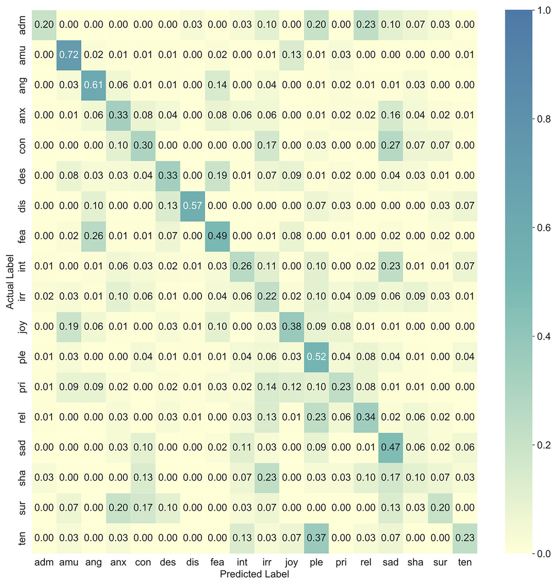
Figure 1: Confusion matrix showing the proportion of responses in the validation set for the best late fusion multimodal classifier (product rule).
Recall rates are shown in the diagonal cells (marked in bold). adm = admiration, amu = amusement, ang = anger, anx = anxiety/worry, con = contempt, des = despair, dis = disgust, fea = panic fear, int = interest, irr = irritation, joy = joy/elation, ple = sensual pleasure, pri = pride, rel = relief, sad = sadness, sha = shame, sur = surprise, ten = tenderness.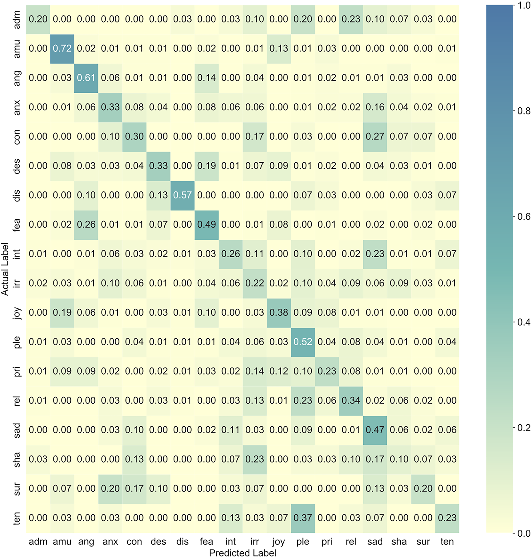
| Classifier | AUC (training) | AUC (validation) |
|---|---|---|
| Maximum Rule | 0.9960 ± 0.0003 | 0.8360 ± 0.0116 |
| Sum Rule | 0.9972 ± 0.0002 | 0.8618 ± 0.0127 |
| Product Rule | 0.9972 ± 0.0002 | 0.8767 ± 0.0135 |
| Weight Criterion | 0.9981 ± 0.0002 | 0.8623 ± 0.0129 |
| Rule-based | 0.9653 ± 0.0015 | 0.8470 ± 0.0176 |
| Elastic Net | 0.9994 ± 0.0000 | 0.8696 ± 0.0168 |
| k-NN | 0.9825 ± 0.0007 | 0.8585 ± 0.0160 |
| Decision Tree | 0.8042 ± 0.0096 | 0.7079 ± 0.0267 |
Note:
Best method is marked in bold.
Early fusion
In this approach, two different input parameter sets were evaluated: an extended set including the eGeMAPS features and AU intensity values and functionals, and a minimal set including the standard GeMAPS features and AU intensity and functionals. These parameter sets were created by concatenating audio and video features and were then used to train distinct classifiers. Table 4 lists the best early fusion multimodal classifiers after hyperparameter tuning. Elastic Net with the extended parameter set performed best, scoring an average validation AUC of 0.8662. As shown in Fig. 2, its intraclass performance was once again better than random guessing for all emotions, and there were also expected confusion patterns such as confusions between joy and amusement and between anger and panic fear.
| Classifier | AUC (train) | AUC (validation) |
|---|---|---|
| Elastic Net (ext.) | 0.9634 ± 0.0024 | 0.8662 ± 0.0150 |
| Elastic Net (min.) | 0.9401 ± 0.0029 | 0.8600 ± 0.0174 |
| k-NN (ext.) | 0.8764 ± 0.0057 | 0.8334 ± 0.0255 |
| k-NN (min.) | 0.8476 ± 0.0077 | 0.8285 ± 0.0259 |
| Decision Tree (ext.) | 0.7772 ± 0.0093 | 0.7320 ± 0.0280 |
| Decision Tree (min.) | 0.7936 ± 0.0130 | 0.7321 ± 0.0376 |
| Random Forest (ext.) | 0.9998 ± 0.0000 | 0.8550 ± 0.0222 |
| Random Forest (min.) | 1.0000 ± 0.0000 | 0.8555 ± 0.0225 |
Note:
ext, extended feature set (eGeMAPS + AUs); min, minimal feature set (GeMAPS + AUs).
Best method is marked in bold.
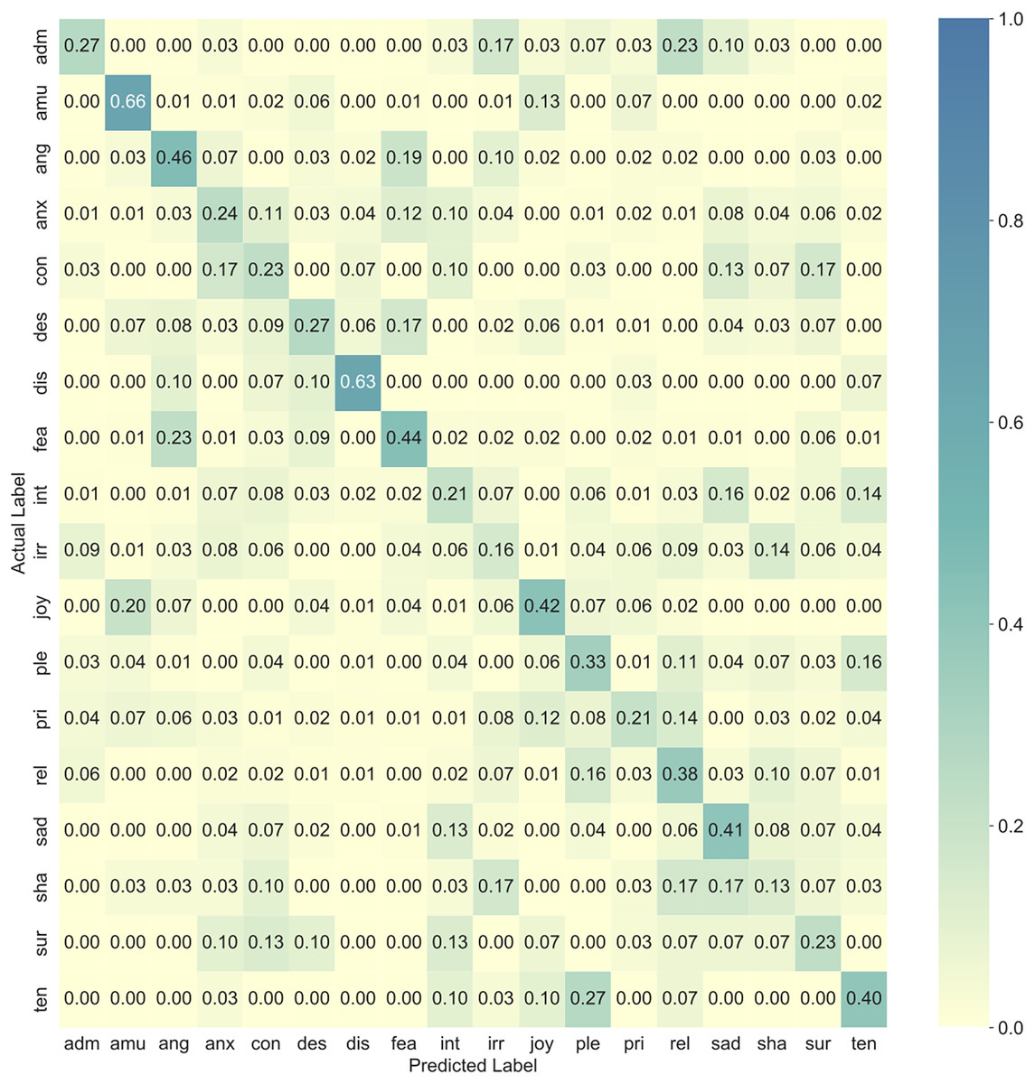
Figure 2: Confusion matrix showing the proportion of responses in the validation set for the best early fusion multimodal classifier (Elastic Net with extended feature set).
Recall rates are shown in the diagonal cells (marked in bold). adm = admiration, amu = amusement, ang = anger, anx = anxiety/worry, con = contempt, des = despair, dis = disgust, fea = panic fear, int = interest, irr = irritation, joy = joy/elation, ple = sensual pleasure, pri = pride, rel = relief, sad = sadness, sha = shame, sur = surprise, ten = tenderness.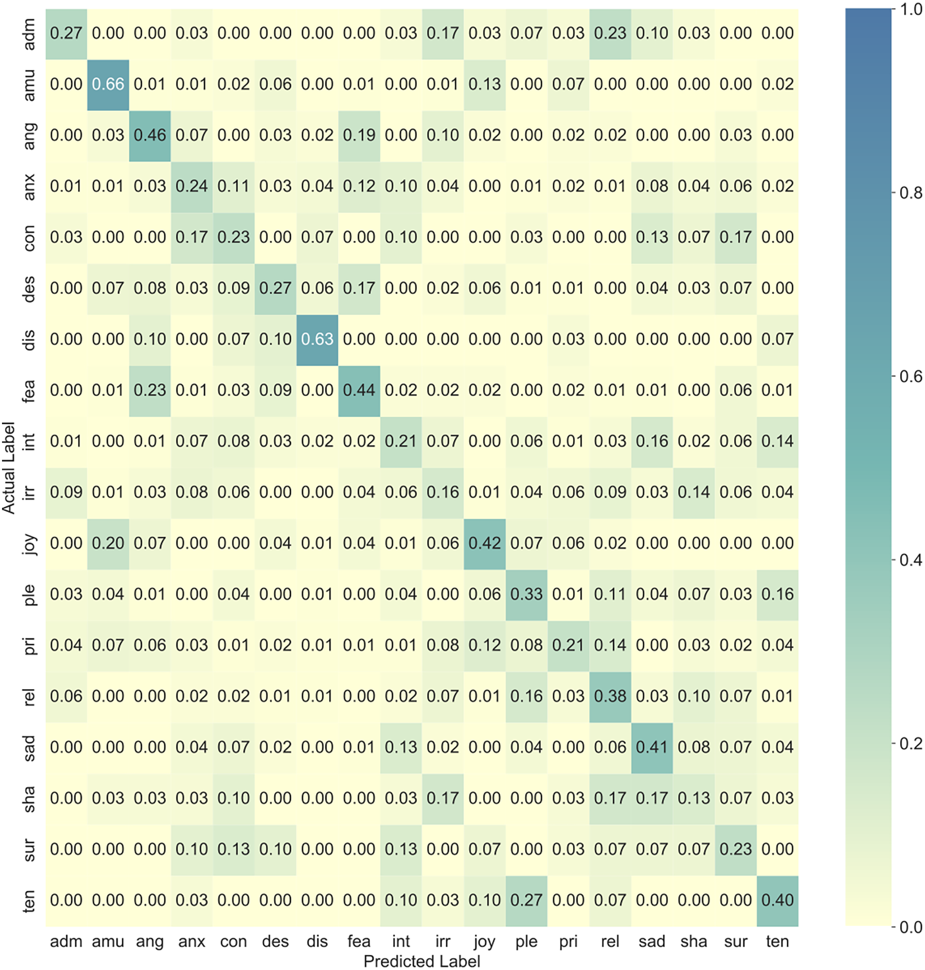
Analyses of feature importance
An in-depth analysis of classifier behavior was conducted by plotting and analyzing the feature importance for each emotion and classifier. Since the input variables were scaled before fitting the model, logistic regression coefficients can be used as feature importance scores for Elastic Nets. A feature is affecting the prediction when its coefficient is significantly different from zero. The probability of an event (emotion) increases and decreases when the coefficient is greater or lower than zero, respectively. The behavior of models based on Random Forest was analyzed using the TreeInterpreter package (Saabas, 2015), which decomposes each prediction into bias and feature contribution components. These contributions were grouped by the predicted emotion and then averaged. The interpretation of feature contribution values coincides with the one explained for Elastic Nets. The contributions of the most important audio features are summarized in Fig. 3, and the full list of importance scores for all audio features and emotions is available in Fig. S7. A summary of the most important video features (Facial Action Units, AUs) is shown in Fig. 4 (with full list shown in Fig. S8). These figures are based on the best performing audio and video classifiers and give a detailed look into which features were important for classification of which emotions. They also represent the best performing multimodal classifier, which was based on late fusion of the best unimodal classifiers using the product rule technique.
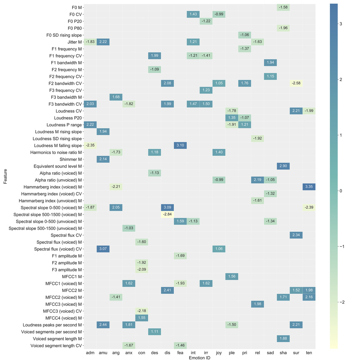
Figure 3: Summary of the most important features (eGeMAPS) for classification of each emotion for the best performing audio classifier (Elastic Net).
See Fig. S7 for a complete list that includes all features. Functionals: M = arithmetic mean, CV = coefficient of variation, P20 = 20th percentile, P80 = 80th percentile, P range = range of 20th to 80th percentile, M/SD rising slope = mean/standard deviation of the slope of rising signal parts, M/SD falling slope = mean/standard deviation of signal parts with falling slope. Features: voiced/unvoiced = feature was based on voiced/unvoiced regions only; F0 = logarithmic fundamental frequency (F0) on a semitone frequency scale; jitter = deviations in individual consecutive F0 period lengths; F1/F2/F3 frequency/bandwidth = centre frequency/bandwidth of the first, second, and third formants; loudness = estimate of perceived signal intensity from an auditory spectrum; harmonics to noise ratio = relation of energy in harmonic components to energy in noise-like components; shimmer = difference of the peak amplitudes of consecutive F0 periods; equivalent sound level = logarithmic average sound pressure level; alpha ratio = ratio of the summed energy from 50–1,000 Hz and 1–5 kHz; Hammarberg index = ratio of the strongest energy peak in the 0–2 kHz region to the strongest peak in the 2–5 kHz region; spectral slope 0–500/500–1,500 = linear regression slope of the logarithmic power spectrum within the two given bands; spectral flux = difference of the spectra of two consecutive frames; F1/F2/F3 amplitude = first, second, and third formant relative energy; MFCC 1–4 = Mel-Frequency Cepstral Coefficients 1–4; loudness peaks per second = number of loudness peaks per second; voiced segments per second = number of continuous voiced regions per second; voiced segment length = length of continuous voiced regions.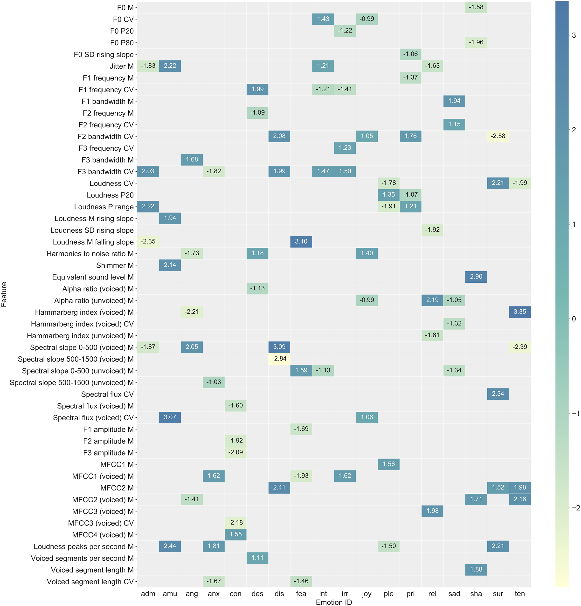
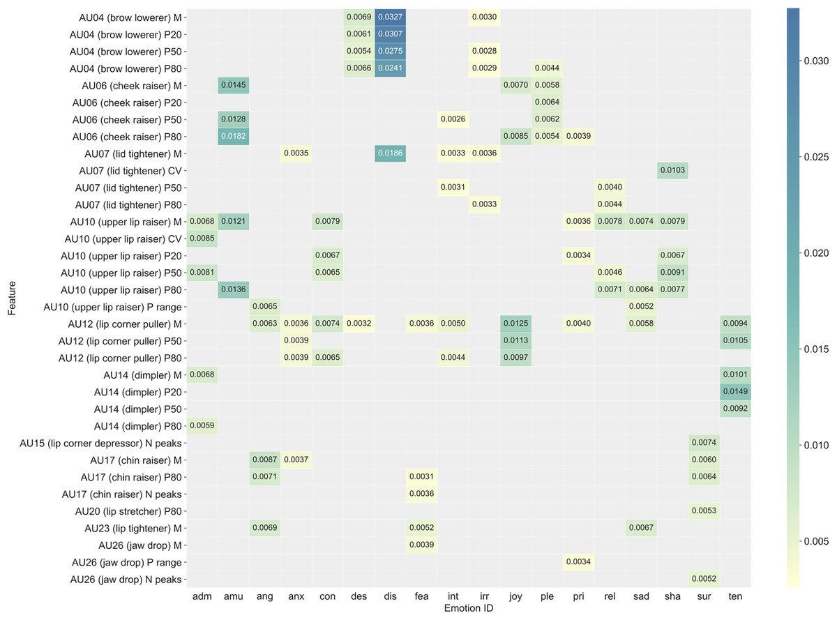
Figure 4: Summary of the most important features (Facial Action Units and functionals) for classification of each emotion for the best performing video classifier (random forest).
See Fig. S8 for a complete list that includes all features. Functionals: M = arithmetic mean, CV = coefficient of variation, P20 = 20th percentile, P50 = 50th percentile, P80 = 80th percentile, P range = range of 20th to 80th percentile, N peaks = number of peaks.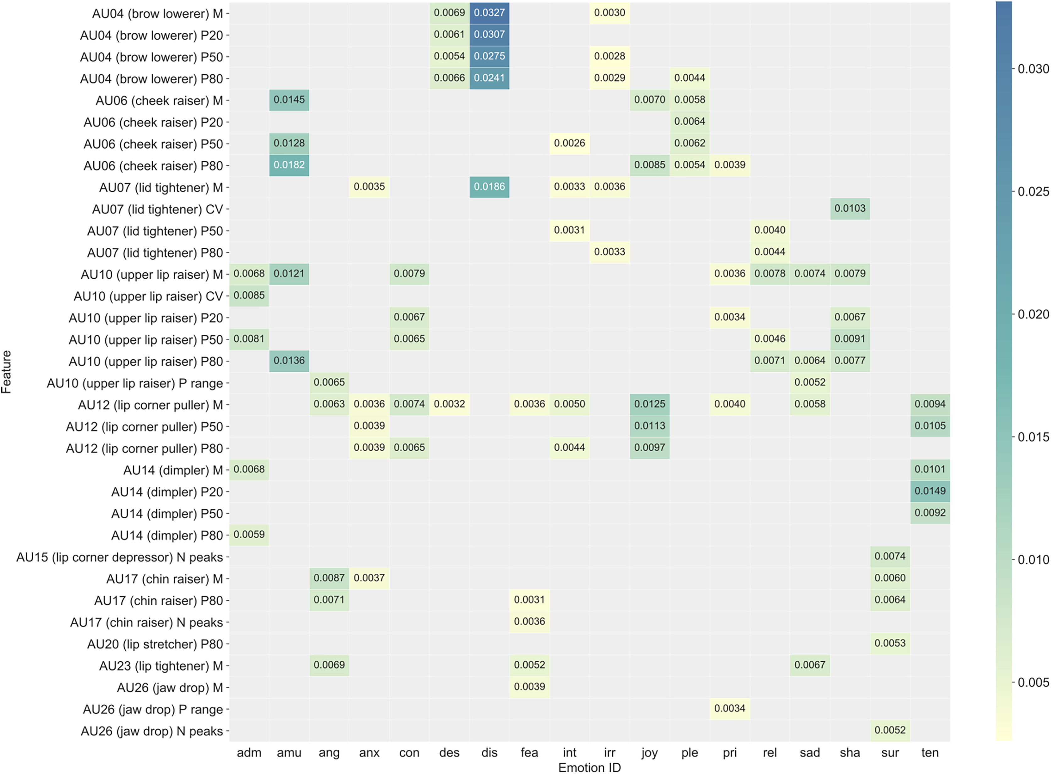
In general, different emotions were associated with different patterns of important features. Important audio features for anger, for example, included spectral balance and amplitude related features that are associated with a “harsh” voice quality (e.g., spectral slope from 0–500 Hz, Hammarberg index, harmonics to noise ratio). Whereas for fear, important audio features included the length of unvoiced segments, amplitude of the first formant frequency, and the mean slope of falling amplitude signal parts. We refer to Eyben et al. (2016) for definitions and calculations of audio features. Important video features included AU12 (lip corner puller) for joy, AU4 (brow lowerer) and AU7 (lid tightener) for disgust, and AU6 (cheek raiser) and AU10 (upper lip raiser) for amusement. For the sake of completeness, the Supplemental Materials also include a summary (Fig. S9) and full description (Fig. S10) of the importance of features for the best early fusion multimodal classification model.
Unsupervised learning
Traditional approach
After determining the optimal number of clusters, these parameters were used as input to k-means and hierarchical clustering. Both clustering techniques were evaluated over the multimodal dataset, with and without dimensionality reduction. Results from the clustering analyses yielded a two-dimensional solution and are shown in Fig. 5.
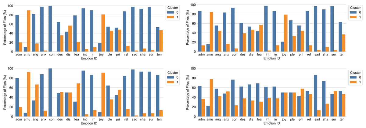
Figure 5: k-Means for k = 2 (top left) and hierarchical clustering for k = 2 and complete distance method (top right) before dimensionality reduction, with percentage of files per emotion and cluster.
The bottom two graphs show k-Means for k = 2 (bottom left) and hierarchical clustering for k = 2 and weighted distance method (bottom right) after dimensionality reduction. adm = admiration, amu = amusement, ang = anger, anx = anxiety/worry, con = contempt, des = despair, dis = disgust, fea = panic fear, int = interest, irr = irritation, joy = joy/elation, ple = sensual pleasure, pri = pride, rel = relief, sad = sadness, sha = shame, sur = surprise, ten = tenderness.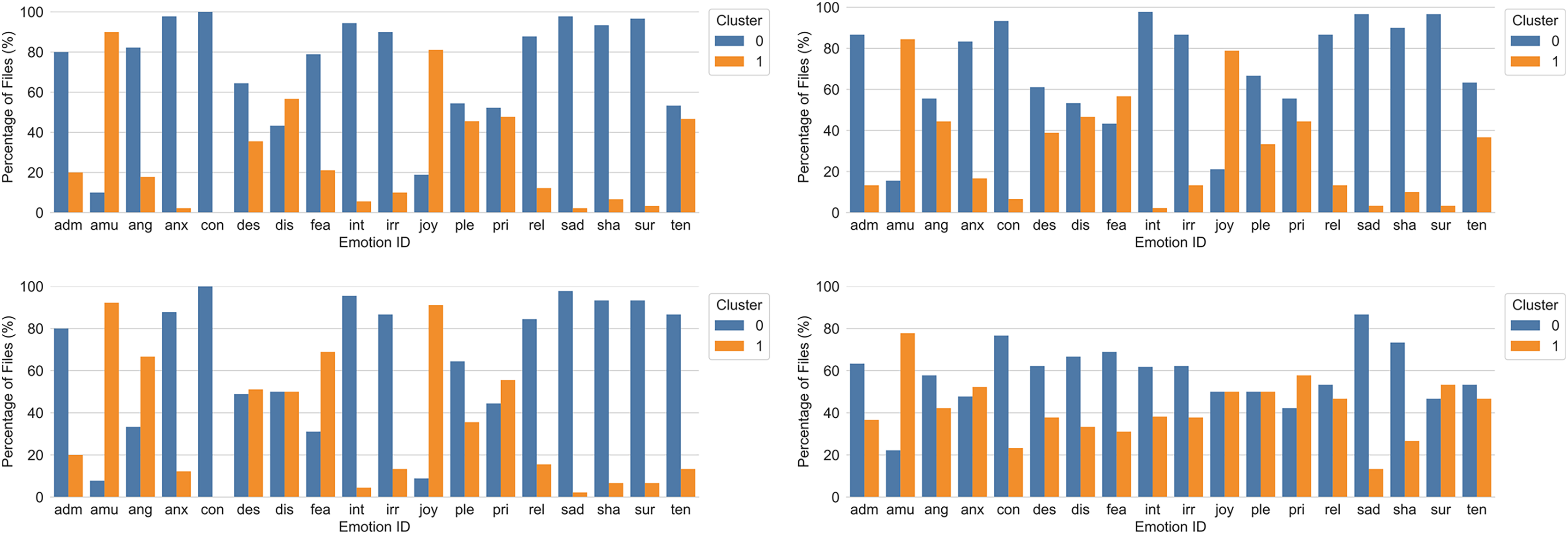
In order to interpret the clusters in terms of underlying features, the problem was analyzed in a supervised manner using Decision Trees. As shown in Fig. 6, the most relevant feature that distinguished between clusters was AU6 (cheek raiser). According to the first decision node, those instances which had an 80th percentile value greater than 0.328 were classified as cluster one. In the next decision node, AU12 (lip corner puller) also contributed, whereas vocal features became more prominent in the third node. These findings were in good agreement with the emotion categories included in cluster one (see Fig. 5), which mainly comprised emotions that are positive (and are characterized by the use of AU6, e.g., amusement and joy; see Fig. S8). The pattern was consistent across both clustering techniques without dimensionality reduction, but changed when the reduced dataset was used for hierarchical clustering (see Fig. 5, bottom right).
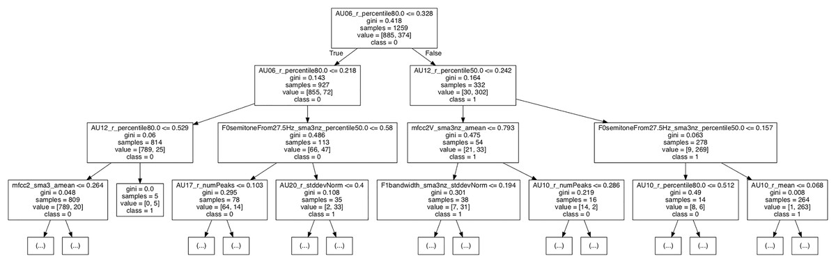
Figure 6: Fragment of the decision tree used to interpret the clustering.
The model was trained on the output of k-Means (k = 2; before dimensionality reduction).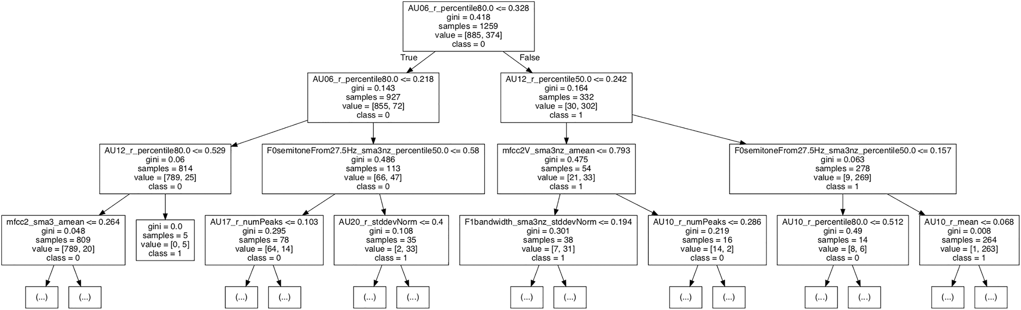
Exploratory approach
After preparing the features and metadata files of the non-reduced multimodal dataset (as described in the “Methods” section), the data was explored in search of meaningful patterns. To this end, three different dimensionality reduction techniques were employed via the TensorFlow Embedding Projector (Wongsuphasawat et al., 2018). The tunable parameters were manually adjusted until any interesting patterns were found. The reader can interactively visualize the data and inspect the results (https://projector.tensorflow.org/?config=https://raw.githubusercontent.com/marferca/multimodal-emotion-recognition/main/4.unsupervised_learning/exploratory_approach/tf_embedding_projector/projector_config.json). Main findings are presented below.
Principal component analysis
Although the projection of data into a two-dimensional space reduced the amount of explained variance to 35%, some interesting patterns were detected. It is apparent from Fig. 7 that the dataset could be split into two clusters. The left and middle side mainly contained high-arousal emotions, such as portrayals of amusement, anger, joy, panic fear, pride, and despair. The right side instead included low-arousal emotions, such as sadness, irritation, interest, anxiety, and contempt. In addition, representations of the same emotion tended to be close to each other.
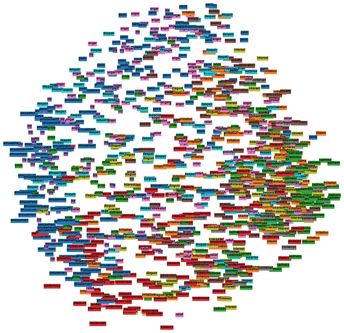
Figure 7: PCA 2D visualization of the multimodal dataset colored by emotion.
Note that 18 non-unique colors were used.
t-SNE
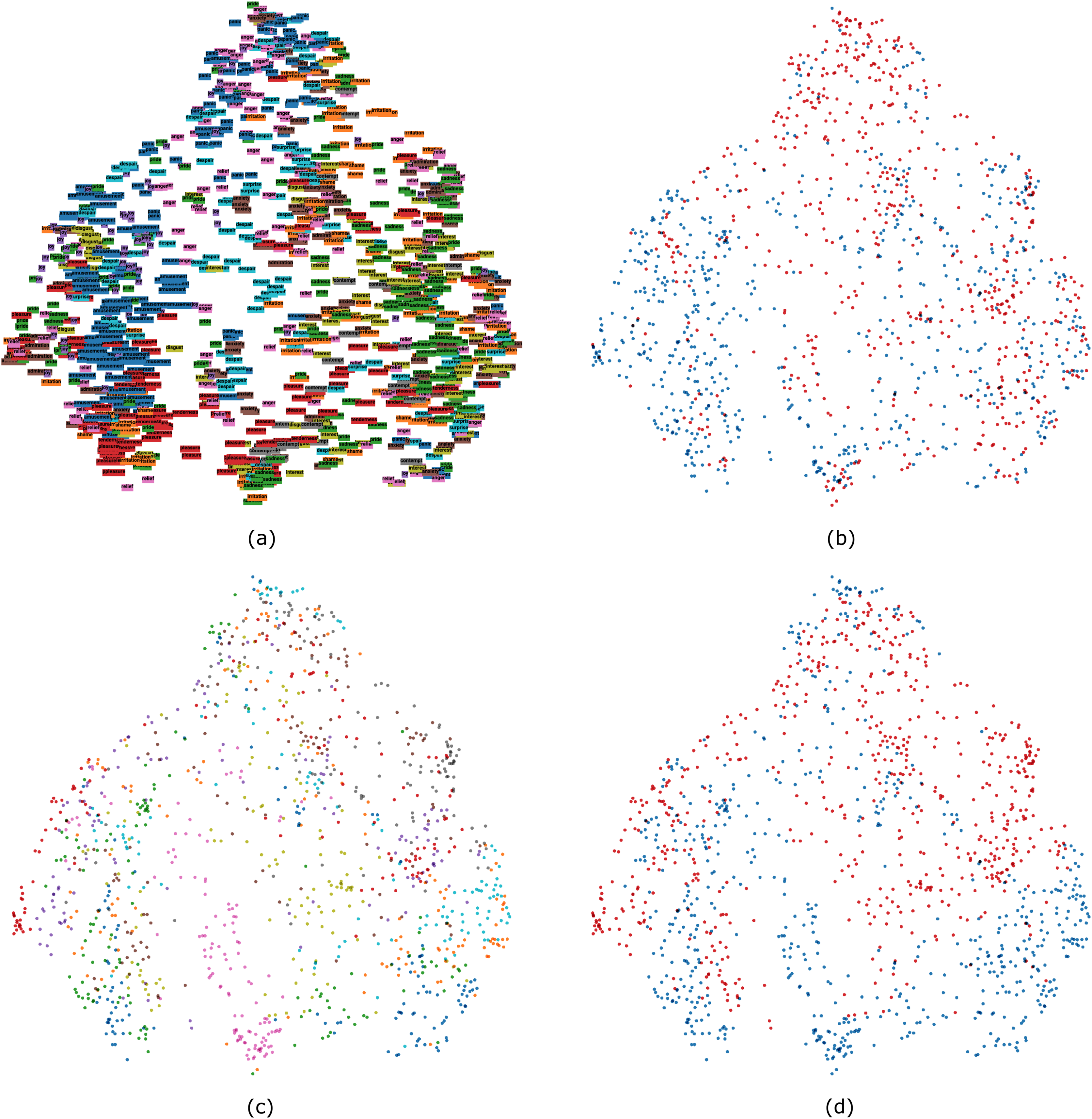
The t-SNE dimensionality reduction technique was run until convergence (6,081 iterations) with a perplexity value of 25 and a learning rate of 10. The data points were then colored by emotion, valence, actor, and actor’s sex. The algorithm grouped the data into three main clusters (Fig. 8), in which emotions characterized by positive valence were grouped together, whereas the rest split into two clusters with high prevalence of panic fear and anger, and of sadness, respectively. Figure 8 also reveals that emotions portrayed by the same actor tended to be close to each other. Something similar also happened when coloring by sex: female samples tended to group together, as did male samples.
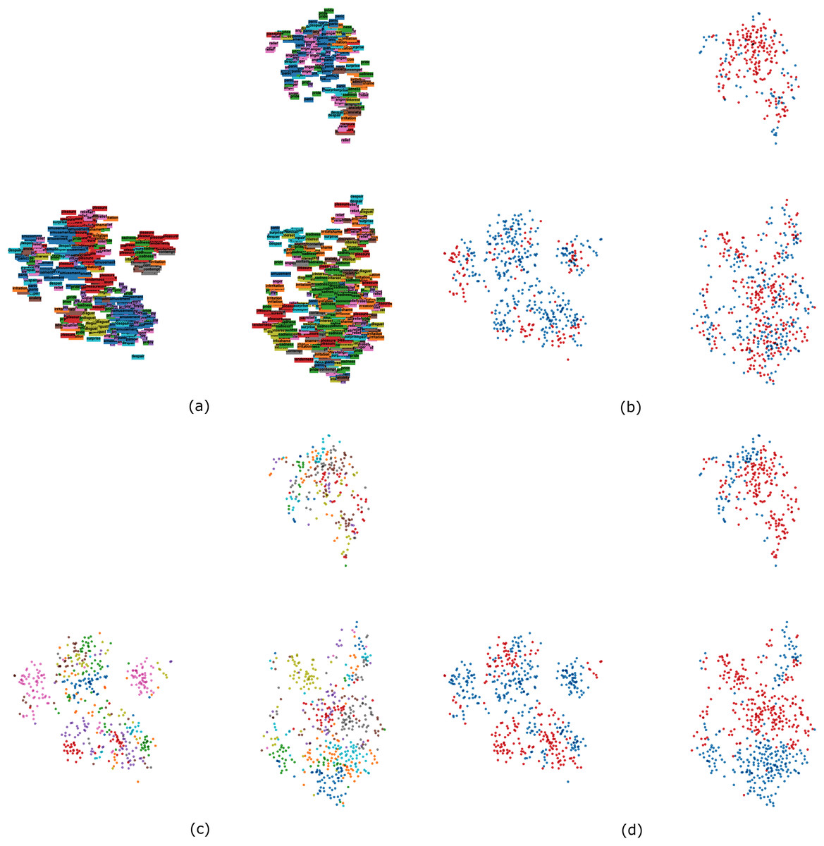
Figure 8: t-SNE 2D visualization of the multimodal dataset colored by emotion (A), valence (B), actor (C), and sex (D).
UMAP
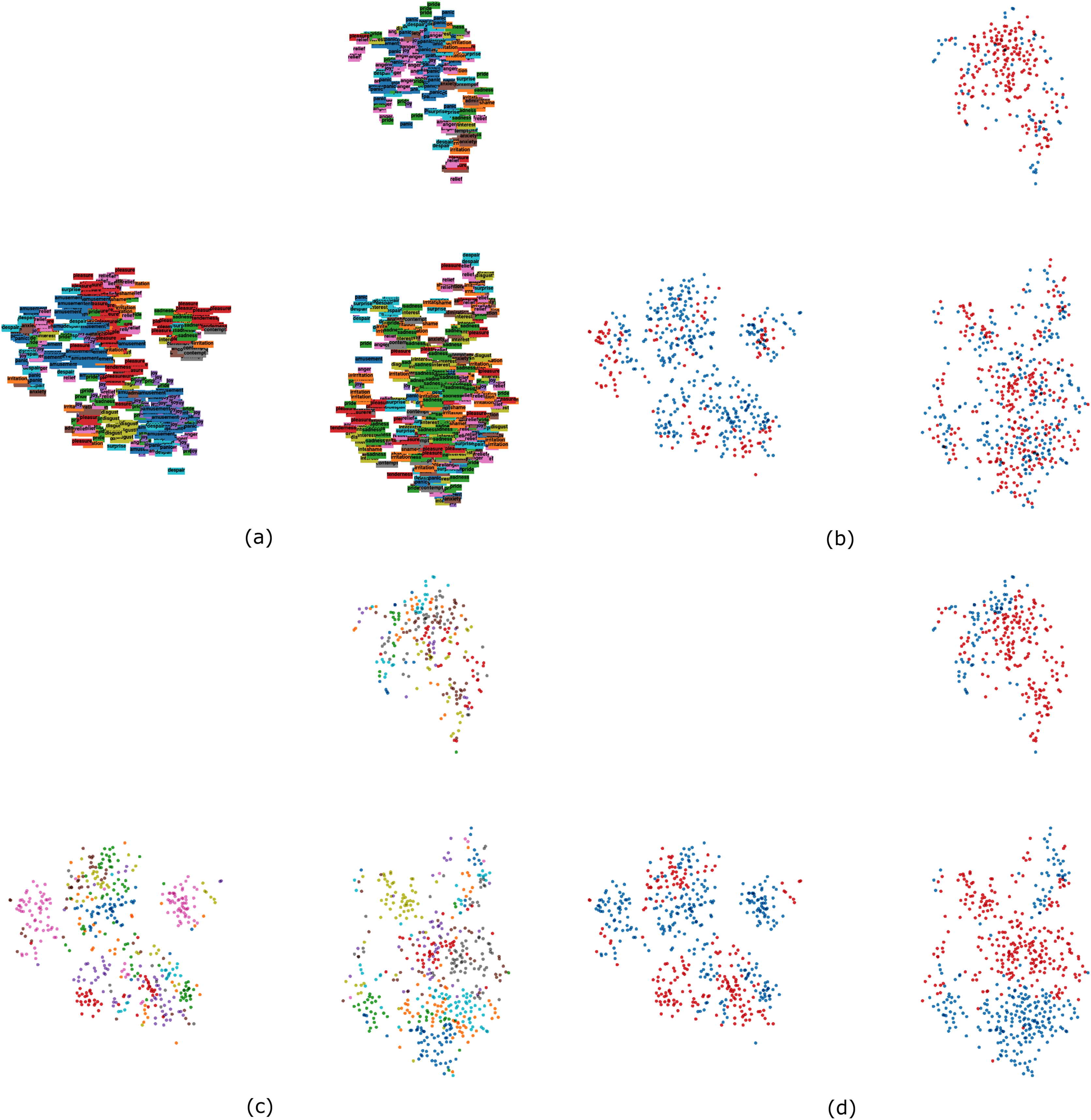
The UMAP algorithm was run for 500 epochs (not a tunable parameter) and 36 neighbors. As shown in Fig. 9, the left side mainly contained high-arousal emotions and positive emotions (e.g., amusement, joy, and despair), whereas the right side contained low-arousal emotions and negative emotions (e.g., sadness, irritation, anxiety, contempt, and interest). Similarly to t-SNE, expressions portrayed by the same actor were close to each other (e.g., actor number 3, pink dots, is a case in point). Finally, Fig. 9 also reveals how the actor’s sex played a part in the clustering results since most of the female and male samples were on the upper and the lower part of the output, respectively.
Figure 9: UMAP 2D visualization of the multimodal dataset colored by emotion (A), valence (B), actor (C), and sex (D).
Discussion
We investigated classification of 18 emotions—portrayed by 10 actors through vocal and facial expressions—using person-independent supervised and unsupervised methods. Our study makes three main contributions to the literature. First, results from the supervised experiments showed that multimodal classifiers performed better than unimodal classifiers and were able to classify all emotions, although recognition rates varied widely across emotions. This indicates that the combinations of vocal and facial features that were used for classification varied systematically as a function of emotion, and that the signal was reliable enough to allow for above chance classification of all 18 emotions. Second, we utilized our machine learning approach to present new data on multimodal feature patterns for each emotion, in terms of the features that contributed most to classifier performance. Third, we explored how wholly unsupervised classifiers would organize the emotion expressions, based on the same features that were used for supervised classification. Several meaningful explanatory patterns were observed and interpreted in terms of valence, arousal, and various actor- and sex-specific aspects. The comparison of supervised and unsupervised approaches allowed us to explore how different methodological choices may provide different perspectives on how emotion expressions are organized.
Overall, the multimodal classifiers performed approximately 5–6% better than the unimodal vocal and facial classifiers in our supervised experiments. The magnitude of this improvement is in accordance with previous studies (see D’Mello & Kory, 2015, for a review). We observed the best performance (AUC = 0.88) for multimodal classifiers that merged the output from the best unimodal vocal (elastic net, AUC = 0.82) and facial (random forest, AUC = 0.80) classifiers using a late fusion approach and the product rule method. A direct comparison with previous classification studies on the GEMEP expression set is difficult because studies have used different classification approaches (e.g., person-independent or person-dependent), algorithms, numbers of emotion categories, and selections of stimuli. Our unimodal vocal and facial classifiers seemed to achieve slightly lower accuracy compared to previous efforts (e.g., Schuller et al., 2019; Valstar et al., 2012), although it must be noted that earlier studies have classified fewer emotion categories. We also used relatively small feature sets, with the aim of mainly including features that are possible to interpret in terms of human perception. For example, we focused on AUs because they provide a comprehensive and widely used way to describe facial expressions (Martinez et al., 2019), that can be used to produce easily interpretable feature patterns for each emotion. However, inclusion of additional features such as head pose and gaze direction would likely increase classification performance. Recent studies have also abandoned the use of pre-defined features altogether and instead use deep learning of physical properties with good results (e.g., Li & Deng, 2020), although such methods often result in features that are difficult to interpret.
Bänziger & Scherer (2010) provided data on human classification for the same stimulus set as used in the current study. Direct comparison of recognition rates is again difficult because the human judgments were collected using different methodology (e.g., judges were allowed to choose more than one alternative in a forced-choice task), but overall our classifiers had somewhat lower recognition rates than the human judges. However, an inspection of recognition patterns showed many similarities between human judges and classifiers. For example, the human judges in Bänziger & Scherer (2010), like our classifiers, received higher accuracy for multimodal vs. unimodal expressions. Looking at individual emotions, human judges showed highest accuracy for amusement, anger, and panic fear. Our classifiers also performed best for amusement and anger, and also performed relatively well for panic fear. Shame received the lowest recognition rates from both human judges and our classifiers. Even confusion patterns showed many similarities between human judges and classifiers. For example, joy and amusement, tenderness and pleasure, relief and pleasure, and despair and panic fear were among the most frequent confusions for both humans and classifiers. Similar recognition patterns for human judges and classifiers tentatively suggest that the included features may also be relevant for human perception of emotion.
Traditional emotion recognition studies using machine learning often aim to achieve the highest possible classification performance, and do not pay attention to feature importance. We propose that a more detailed inspection of feature importance presents a promising method for investigating emotion-related patterns of probabilistic and partly redundant vocal and facial features. Such patterns may be difficult to discover using traditional descriptive statistics and linear analyses. We present detailed multimodal feature patterns for each of the 18 included emotions, several of which have rarely been included in previous emotion expression studies (e.g., Figs. 3 and 4). Future studies are needed to investigate how well the obtained patterns may generalize to other data sets and other classification methods.
We also performed a number of unsupervised classification experiments, guided by the idea that they may provide additional information about how emotion expressions are organized (e.g., Azari et al., 2020). Previous studies on the organization of emotion expressions have focused on human perception (e.g., Cowen et al., 2019), whereas our study instead investigated the organization of emotion expressions based on their physical vocal and facial properties. Results from these experiments did not replicate a structure with 18 emotion categories. This was expected because such a solution would require that almost all of the variance in the included features would be explained by emotion expressions. However, all methods lead to meaningful structures that could often be interpreted in relation to emotion categories. Traditional methods based on k-means and hierarchical clustering proposed a two-factor solution which was interpreted using decision trees. This approach revealed that AU6 (cheek raiser) was the most relevant feature at the first decision node. This guided our interpretation of the two clusters as largely representing positive and negative valence, although expressions of negative emotions that shared key features with positive emotions did also end up in the ‘positive’ cluster. The exploratory dimension reduction methods gave further insights. PCA results could largely be interpreted in terms of high vs. low arousal expressions, although Fig. 7 also revealed that portrayals of the same emotion tended to be close together. Results from the t-SNE and UMAP analyses could also be interpreted in terms of arousal, valence, and emotion—but they also revealed that person and gender specific aspects contributed to clustering. For example, portrayals from the same actor tended to be close to each other, as did portrayals by male and female actors, respectively (see Figs. 8 and 9). One conclusion that can be drawn is that both emotional and non-emotional variability is likely to play a role in unsupervised classification of emotions (see Li & Deng, 2020), especially in person-independent approaches where within-person normalization of features is often not a feasible solution. Future research could focus on ways to minimize the impact of feature variability that is not directly related to the expression of emotions.
Our stimuli consisted of actor portrayals recorded in a studio, so future research is required to investigate which of the results will generalize to naturalistic conditions. Studies using spontaneous expressions are important because recent research suggests that there may be small but systematic differences between how emotions are conveyed in actor portrayals vs. spontaneous expressions (e.g., Juslin, Laukka & Bänziger, 2018; Krumhuber et al., 2021a). Another limitation of our study was that we did not fully take advantage of the dynamic nature of the stimuli, and only used such temporal dynamics information that was directly encoded in the features. Future studies could instead track the dynamic changes of features over time and use analysis methods that take advantage of this information (e.g., long short-term memory recurrent neural networks; see Wöllmer et al., 2013; Zhao et al., 2019). While the GEMEP data set is relatively small, openly available huge data sets could in the future enable modeling of emotion expressions via transformers and attention-based mechanisms (e.g., Siriwardhana et al., 2020; Vaswani et al., 2017). Even for moderately sized data sets, such modeling could be useful, as we have recently shown in another context (Gogoulou et al., 2021).
With an increase in the number of human-robot interactions with an emotional component (Shum, He & Li, 2018)—e.g., recognizing an angry customer in dialog with a chatbot—the future will hold more opportunities for data-driven reasoning. Besides software robots, there is also an increase in the number of filmed interactions between humans and physical robots and corresponding studies of human-robot cooperation (Crandall et al., 2018). Studies into unlabeled data from such sources can be done using self-supervised learning. Such studies may assist in understanding the importance of correctly interpreting emotions, and will likely also become more common and potentially have important societal implications. This further motivates deep dives into the methodology, of the kind that we have attempted here.
Conclusions
We propose that research on emotion expression could benefit from augmenting supervised methods with unsupervised clustering. The combination of methods leads to more insight into how data is organized, and we especially note that the investigation of explanatory patterns could be a valuable meta-heuristic that can be applied to several classification areas. We believe that advances in the basic science of understanding how emotions are expressed requires continued efforts regarding both the development of more representative stimulus materials and of more representative vocal and facial features. Machine learning methods could play a vital role in the study of how emotions are expressed nonverbally through the voice and the face.