
Experimental interpretation of adequate weight-metric combination for dynamic user-based collaborative filtering
- Published
- Accepted
- Received
- Academic Editor
- Zhiwei Gao
- Subject Areas
- Data Mining and Machine Learning, Data Science
- Keywords
- Collaborative filtering, Dynamicity, MovieLens dataset, Recommender systems, Significance weighting, Test item bias, User-based neighborhood
- Copyright
- © 2021 Okyay and Aygun
- Licence
- This is an open access article distributed under the terms of the Creative Commons Attribution License, which permits unrestricted use, distribution, reproduction and adaptation in any medium and for any purpose provided that it is properly attributed. For attribution, the original author(s), title, publication source (PeerJ Computer Science) and either DOI or URL of the article must be cited.
- Cite this article
- 2021. Experimental interpretation of adequate weight-metric combination for dynamic user-based collaborative filtering. PeerJ Computer Science 7:e784 https://doi.org/10.7717/peerj-cs.784
Abstract
Recommender systems include a broad scope of applications and are associated with subjective preferences, indicating variations in recommendations. As a field of data science and machine learning, recommender systems require both statistical perspectives and sufficient performance monitoring. In this paper, we propose diversified similarity measurements by observing recommendation performance using generic metrics. Considering user-based collaborative filtering, the probability of an item being preferred by any user is measured. Having examined the best neighbor counts, we verified the test item bias phenomenon for similarity equations. Because of the statistical parameters used for computing in a global scope, there is implicit information in the literature, whether those parameters comprise the focal point user data statically. Regarding each dynamic prediction, user-wise parameters are expected to be generated at runtime by excluding the item of interest. This yields reliable results and is more compatible with real-time systems. Furthermore, we underline the effect of significance weighting by examining the similarities between a user of interest and its neighbors. Overall, this study uniquely combines significance weighting and test-item bias mitigation by inspecting the fine-tuned neighborhood. Consequently, the results reveal adequate similarity weight and performance metric combinations. The source code of our architecture is available at https://codeocean.com/capsule/1427708/tree/v1.
Introduction
Recommender systems (RS) are utilized in various applications, and users interact with them on a range of application-specific platforms. Personal data and previous activities are combined to understand a user’s taste. Any recommendation of items on a platform can be provided. Considering both online and offline applications, a stable architecture is essential for machine learning and for promoting the business of any platform. Recommender systems have been implemented on various platforms, including social media (Kazienko, Musiał & Kajdanowicz, 2011), healthcare (Calero Valdez & Ziefle, 2019), journals (Wang et al., 2018), music (Andjelkovic, Parra & O’Donovan, 2019; Celma & Herrera, 2008), suggestion systems, and movie recommendation frameworks (Moreno et al., 2013; Isinkaye, Folajimi & Ojokoh, 2015; Wang, Wang & Xu, 2018). Recommender systems focus on analyzing preferences and deciding the prospective action of a user. A person performs activities (such as passing remarks, leaving comments, giving rates, liking, or disliking products) on a specific application because these activities are all logged into a database. Movie-based RS has been the focus of many data scientists for two significant reasons. First, scientific datasets such as MovieLens (Grouplens, 1992) and Netflix (Netflix, 2009) are readily available and easy to use. Second, an overall RS architecture has been established that is entirely compatible with additional user and item features, enabling scientists to measure two well-known phenomena in collaborative filtering (CF): (i) user-based similarity and (ii) item-based similarity.
This study aims to measure the effect of correlation adjustment. Considering the literature, there are many reported RS implementations; however, it is unclear how the inclusion or exclusion of a test item is determined during statistical parameter computations. Similarity calculations between two users require analytical computations, such as the mean and median. Theoretical studies may set statistical arguments as global parameters to encapsulate computations for all upcoming test attempts concerning time complexity and memory management. Although setting parameters globally is computation-friendly, if all statistical primitives are set in this wide scope, test items become less dependent on the related test attempts. Hence, the expected recommendation may be slightly false. Considering real-time applications, the rating value of the recommended item is unknown. In this study, the dynamic effect of the item-of-interest (IOI) is examined to demonstrate the difference between theoretical and real-time performance. In addition, the co-rated item count (CIC) between the user-of-interest and its neighbors is utilized to revise the calculated similarity weight for further constant multiplications (Ghazanfar & Prugel-Bennett, 2010; Levinas, 2014; Zhang & Yuan, 2017; Gao et al., 2012; Bellogín, Castells & Cantador, 2014; Zhang et al., 2020). Thus, the correlation between users is connected to the commonly rated item counts. We refer to this multiplication as the CIC-based significance weighting (SW) method by demonstrating its performance. We interpret the efficiency of the IOI and SW conditions based on four different similarity equations, including Pearson similarity, median-based robust correlation, cosine similarity, and Jaccard similarity.
In general, studies have focused on finding ways to increase the efficiency of RS. The closer the forecast is to the user preference obtained, the more accurate the system design is. However, the performance metrics of a system can be more than a single prediction accuracy. In this study, we examined previously proposed similarity equations and performance metrics. The research constructs a perspective on how to connect user similarity measurements to an enlarged number of performance metrics, including those from other disciplines. Schröder, Thiele & Lehner (2011) propose the utilization of relatively less known metrics such as informedness, markedness, and Matthews correlation because they are superior to precision, recall, and F1-measure. Schröder, Thiele & Lehner (2011) acknowledge that these performance metrics are suitable for determining the top-n recommendation in e-commerce applications; therefore, we evaluate the performance of these metrics compared to the well-known ones.
Previous RS implementations have either a relatively small set of metrics for testing (Feng et al., 2018; Bag, Kumar & Tiwari, 2019; Li et al., 2014; Nguyen et al., 2020) or a limited range of specific parameters, such as the best neighborhood (Ghazanfar & Prugel-Bennett, 2010; Arsan, Koksal & Bozkus, 2016; Sánchez et al., 2008; Liu et al., 2013; Huang & Dai, 2015; Sun et al., 2017). Any user is provided with a recommendation by examining the closest neighbors who have the same tendencies for the related IOI. Instead of setting the best neighbor count ( ) to a constant value, the neighborhood should be appropriately determined. Therefore, we parameterize the number of neighbors, s.t., using step size between the least neighbor count ( ) and most neighbor count ( ).
A comprehensive back-end software architecture has been developed in this study. Our framework1 is an adaptive tool that enables the test environment to capture the general behavior of high-density datasets with an adjusted .
To the best of our knowledge, no previous studies on RS have extensively focused on an adequate combination of similarity measurements and performance metrics. Overall, the following highlights are presented in the scope of this study.
-
We construct an RS framework that highlights the possible pitfalls and enhancements in RS architectural designs. Therefore, the following two perspectives are applied to the similarity equations.
The first perspective underlines the dynamicity principles of real-time systems by excluding the IOI, known as no item-of-interest (nIOI).
The second perspective emphasizes the results of the utilization of significant weights. Considering the SW method, the more common the rating counts from neighbors observed are, the more significant the weights.
The is analyzed and determined experimentally considering a number of performance metrics.
Extensive tests are applied to popular MovieLens releases with randomized trials of separate runs.
Considering the evaluation, relatively less known performance metrics such as informedness, markedness, and Matthews correlation are examined comprehensively. In addition, established metrics such as precision, sensitivity, specificity, F1-measure, fallout, miss rate, etc., including error metrics, are compared. These prediction-oriented metrics have been extensively demonstrated with notable outcomes.
Prevalence threshold and threat score, which are frequently practiced in other disciplines, are analyzed in the context of RS.
Finally, the heat-map tables for the top-performing s connected to the adequate weight-metric combinations are presented.
The brief of the overall paper structure and each subsection content are visually presented in Fig. 1. The remainder of this study is organized as follows. The materials and methods are provided in Section “Materials and Methods”, wherein the nomenclature and dataset details are presented. In addition, similarity equations and performance metrics used throughout this study are presented in the same section. Section “Experimental Design” includes the details of the computation environment and preliminary selection of top-performing neighbors. This is followed by the extensive results in Section “Results and Discussion”. In the last section, the conclusion and recommendations for future research are presented.
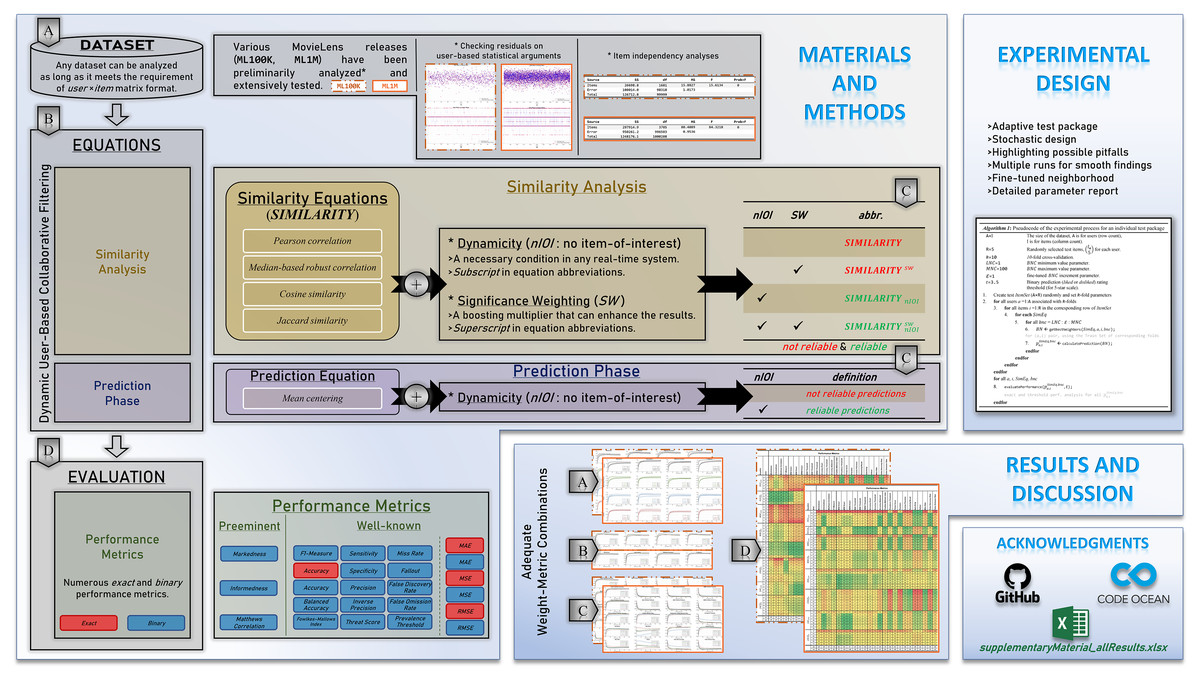
Figure 1: Depiction of the paper structure, technical summary, and contributions.
Materials and Methods
This section describes the dataset used and the methods applied. First, the technical details of MovieLens releases are provided. Thereafter, the touchstone similarity equations and the modifications, considering the nIOI phenomenon and SW, are discussed. Finally, the performance metrics implemented in the proposed RS framework are presented. The symbols and abbreviations used throughout this study are listed in Table 1.
| Symbol/Abbreviation | Explanation |
|---|---|
| User-of-interest | |
| User-of-interest where test item bias is discarded | |
| Any item-of-interest | |
| Possible nominees to be a neighbor | |
| Any possible neighbor for collaboration | |
| Sorted and selected neighbor | |
| Rating vector of for all items | |
| Rating of u for i | |
| The mean of given ratings for u | |
| The median of given ratings for u | |
| The rating history of u | |
| Pearson Correlation Coefficient | |
| Median-based Robust Correlation coefficient | |
| COSine similarity | |
| JACcard similarity | |
| Similarity weight between a and u for equation , where can be given similarity equations | |
| The rating prediction of a for i | |
| Co-rated Item Count between two users | |
| True Positive | |
| True Negative | |
| False Positive | |
| False Negative |
A. The MovieLens
Considering the current RS applications, the basic practical structure of data commonly has a user × item matrix format. One of the frequently trained scientific datasets is MovieLens (Harper & Konstan, 2015) which has several releases based on size and additional content.
Considering Table 2, the main types of MovieLens can be reviewed depending on the rating size. For example, ML100K has 100,000 clicks. The MovieLens dataset is upgraded several times for the expanded types and for the versions of previous releases. For instance, the ML100K type has various releases, such as one that includes one to five ratings with only decimal values. The latest ML100K version consists of 0.5 steps between ratings, including half stars. However, this version is not recommended for shared research results because it is a developing dataset. Several previous studies focused on the tried-and-trusted original ML100K release, which is a pioneering collection and has considerably efficient runtime performance. Considering the scope of this study, we utilize this original release, which includes only full stars. Additionally, we encapsulated extensive experiments of ML1M to maintain full-star rating scaling parallelism with the ML100K. Therefore, we comparatively present the results related to the original ML100K and ML1M.
| Releases | ML100K | ML1M | ML10M | ML20M | ML25M |
|---|---|---|---|---|---|
| Number of Ratings | 100,000 | 1,000,209 | 10,000,054 | 20,000,263 | 25,000,095 |
| Number of Users | 943 | 6,040 | 69,868 | 138,493 | 162,541 |
| Number of Movies | 1,682 | 3,706 | 10,681 | 27,278 | 62,423 |
| Timespan | 09/1997–04/1998 | 04/2000–02/2003 | 01/1995–01/2009 | 01/1995–03/2015 | 01/1995–11/2019 |
| Miscellaneous Information | At least 20 ratings by each user, simple demographic information for users (age, gender, occupation, zip-code). 5-star rating. | At least 20 ratings by each user, simple demographic information for users (age, gender, occupation, zip-code). 5-star rating. | At least 20 ratings by each user. No demographic information. Each user is represented by only an ID. 5-star rating with half-stars. |
At least 20 ratings by each user. No demographic information. Each user is represented by only an ID. 5-star rating with half-stars. |
At least 20 ratings by each user. No demographic information. Each user is represented by only an ID. 5-star rating with half-stars. |
In this section, preliminary dataset analyses are presented. To validate the methods used in the following sections, residual checks on user-based statistical arguments and item-based independence analyses were performed as follows.
(1) Checking residuals on user-based statistical arguments
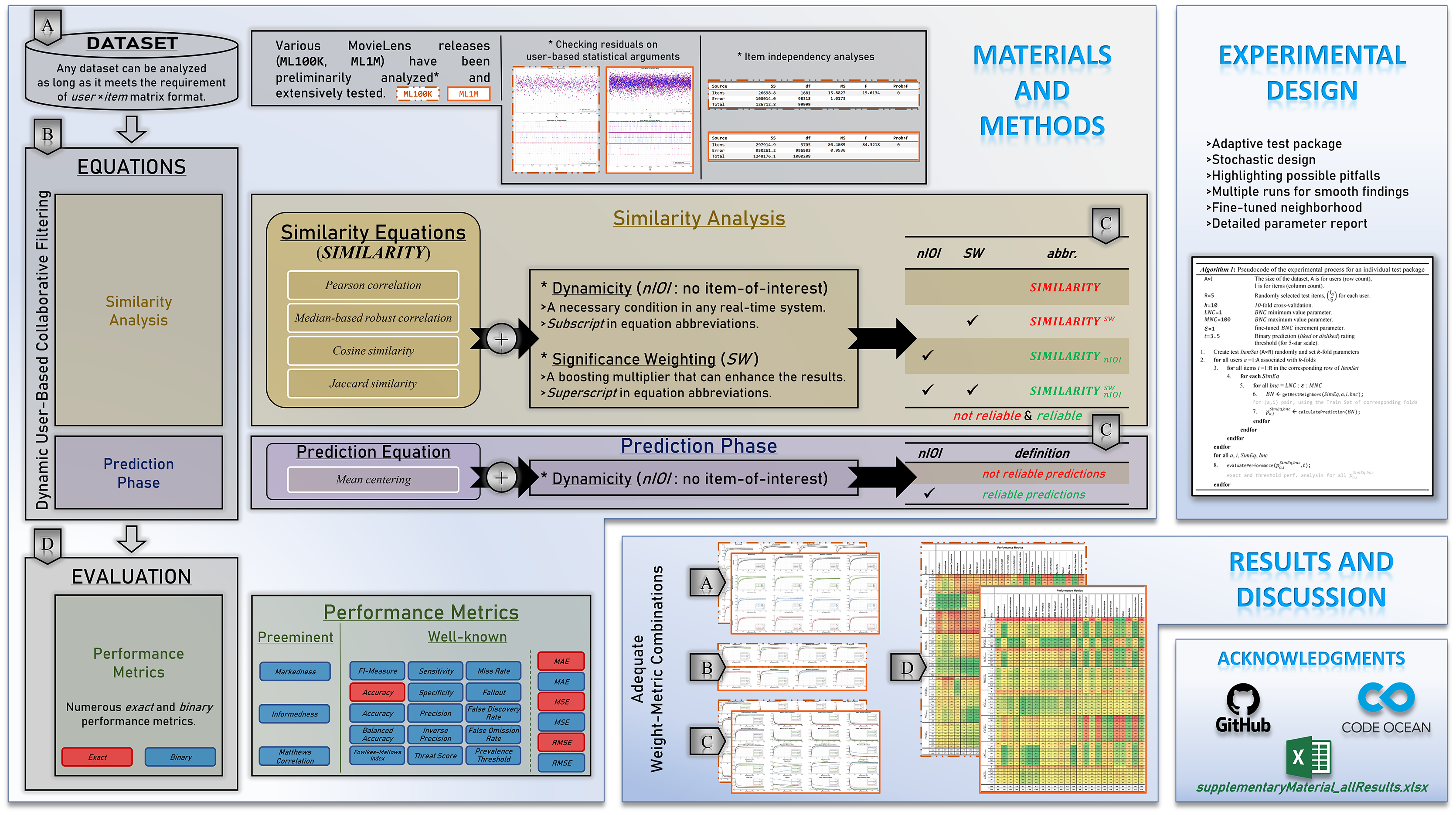
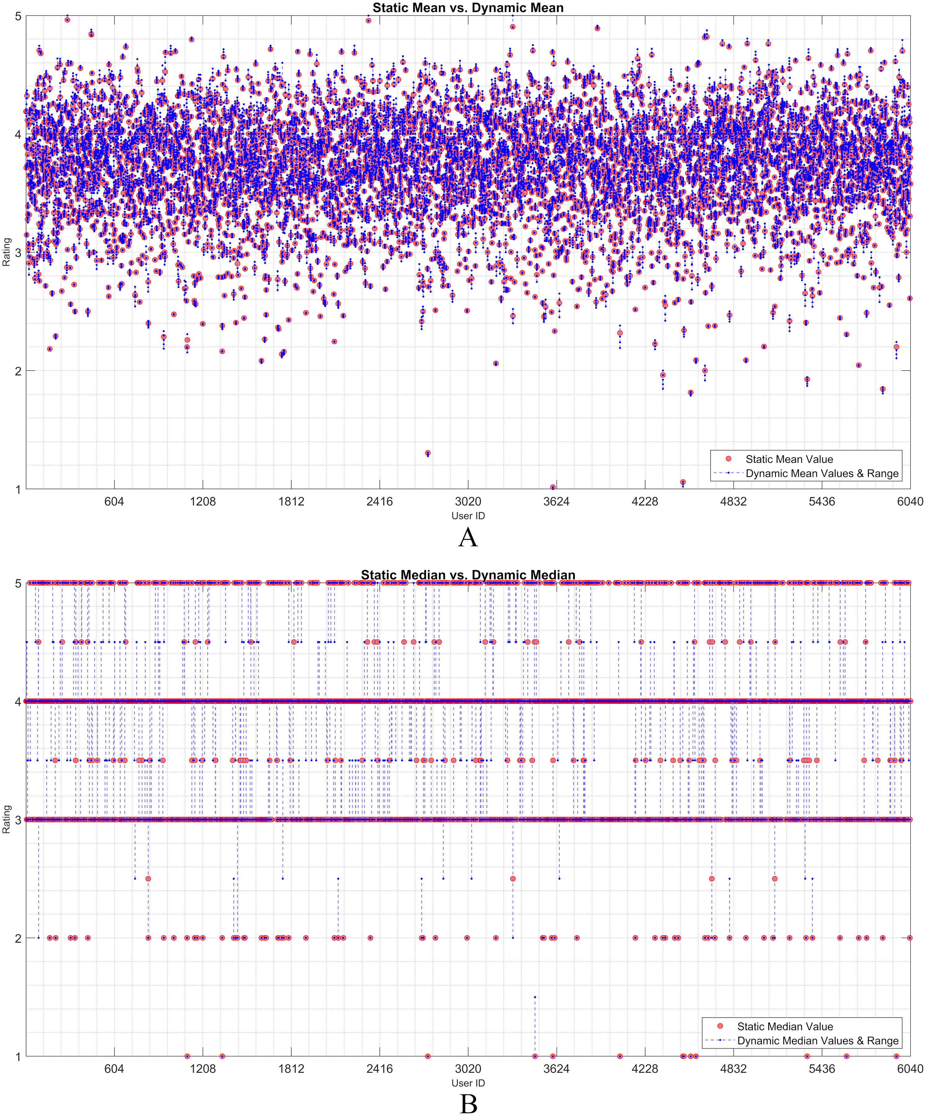
The dynamicity effect of user-based statistical arguments (such as the mean and median) is discussed in this subsection. As static and dynamic approaches are the main focus, a visualization of their residual analysis on the utilization of the arguments is presented. Therefore, the rating history of each user was examined based on the statistical observations. Considering any user, it is observed that the statistical values of all the ratings change when an item is assumed as unrated. The IOI values that are individually excluded from the user vector are dynamically processed. The effect of each discarded rating was recorded as a residual over the dynamic mean or median. Thereafter, the static observation and dynamic approach were evaluated using the residual approach.
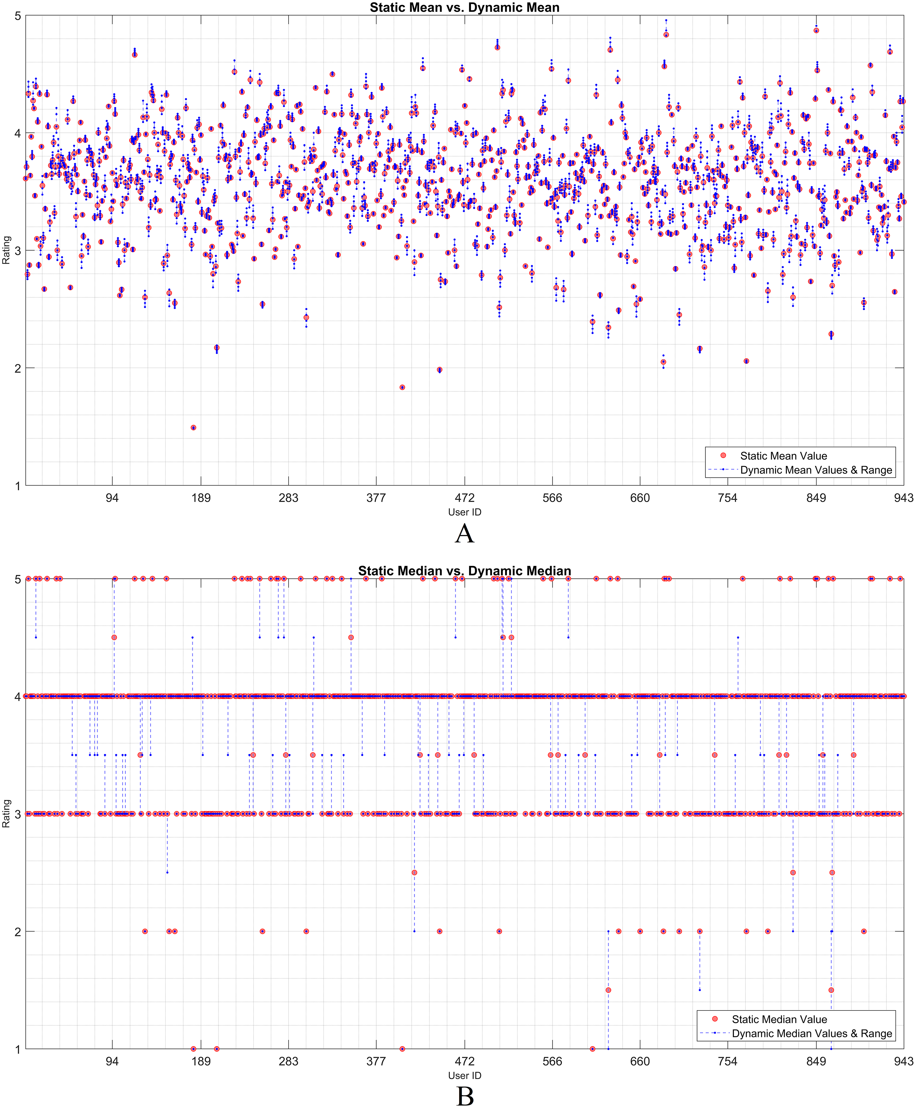
Figures 2 and 3 show the static and dynamic analyses based on the (A) mean and (B) median usage based on the ML100K and ML1M releases, respectively. The x- and y-axis show the user ID and unique rating values, respectively. Each red dot statically indicates the mean or median values of all user ratings, whereas the blue dots show the deviation of the unit ratings from the static value. It may be observed in the median analysis that the blue dots were aggregated, while the outliers in the datasets were suppressed, indicating the superiority of the median over the mean in the presence of outliers.
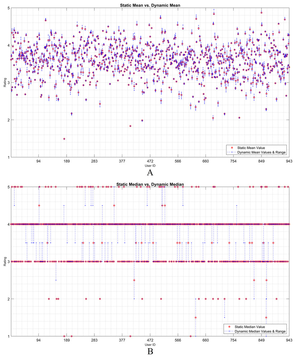
Figure 2: User-based (A) mean & (B) median residuals on static vs. dynamic conditions: ML100K.
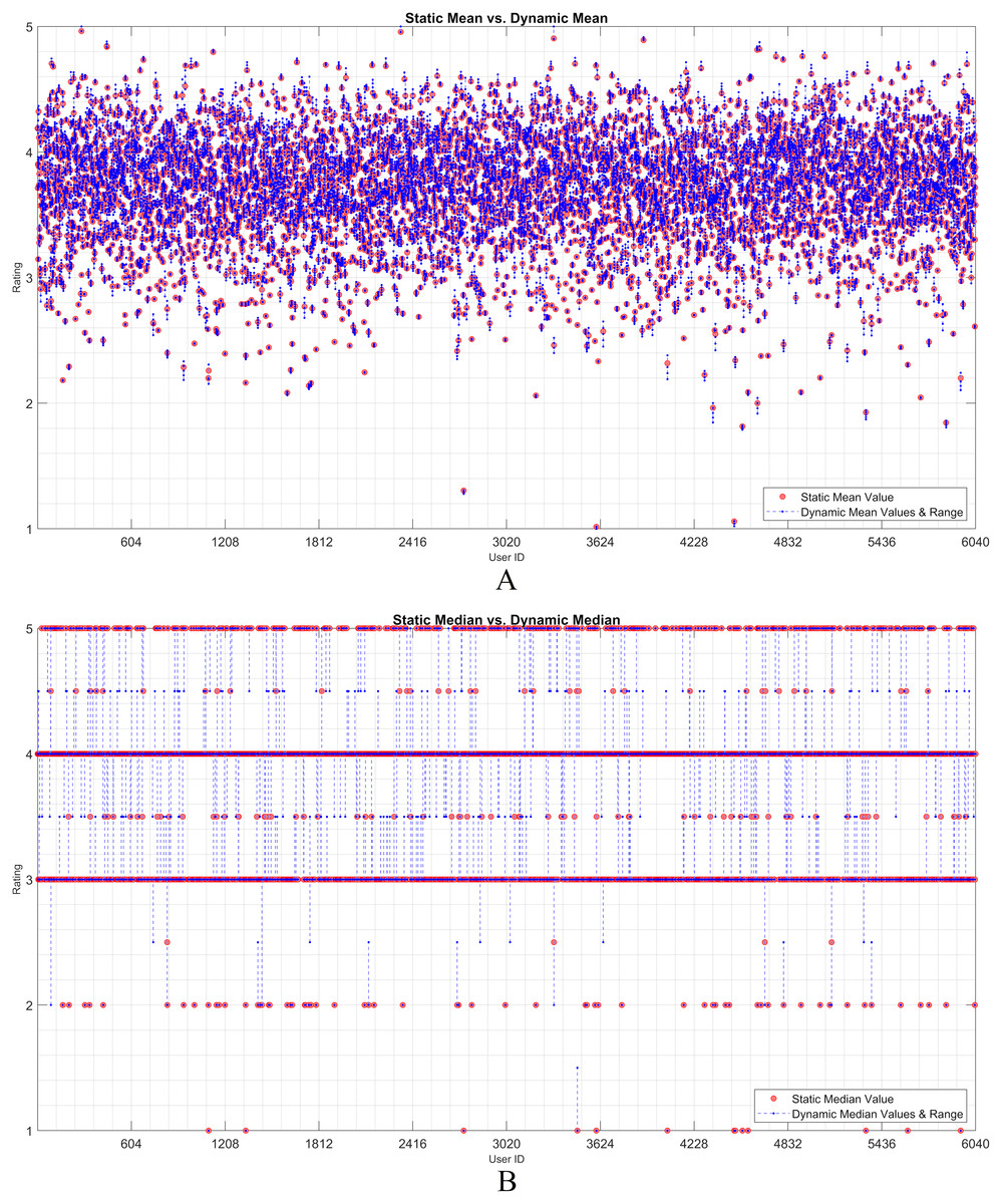
Figure 3: User-based (A) mean & (B) median residuals on static vs. dynamic conditions: ML1M.
(2) Item independency analyses
Considering the dynamic approach regarding real-time systems, excluding the IOI in the users’ statistical calculations depends on the item’s independence condition. Therefore, each particular item in the datasets was analyzed based on the independence. The leave-item-out approach emerges as a useful method because the items are independent of each other. Consequently, an item-based one-way analysis of variance (ANOVA) was performed. Each column (i.e., each item) was subjected to testing in the user × item matrix, validating their independencies. The ANOVA provides information about inter- and intra-group variations. By calculating the sum of squares (SS), degrees of freedom (df), and mean squared errors (MS), the F-test (the ratio of inter- and intra-group variability) is applied. Considering Tables 3 and 4, an analysis of the ML100K and ML1M releases is presented. The validity of item independence is proven by both the and probability (P) values, which are obtained from the F-distribution. The lower the P-values, the higher the chances of strong evidence against the null hypothesis. P-values (significance level) were obtained, indicating that the null hypothesis is rejected.
| Source | SS | df | MS | F | Prob>F |
|---|---|---|---|---|---|
| Items | 26,698.8 | 1,681 | 15.8827 | 15.6134 | 0 |
| Error | 100,014.0 | 98,318 | 1.0173 | ||
| Total | 126,712.8 | 99,999 |
| Source | SS | df | MS | F | Prob>F |
|---|---|---|---|---|---|
| Items | 297,914.9 | 3,705 | 80.4089 | 84.3218 | 0 |
| Error | 950,261.2 | 996,503 | 0.9536 | ||
| Total | 1,248,176.1 | 1,000,208 |
B. Similarity and prediction equations
The four touchstone similarity equations and prediction formula are considered in this section. Before the technical statements, an overview of the application perspective of the touchstone equations is provided.
is within the scope of several studies. Music RS is among the most common applications (Kuzelewska & Ducki, 2013). In particular, considering music genre recommendations, has attracted attention. Additionally, there are other applications. Mukaka explains the management of medical data based on the utilization of (Mukaka, 2012), as in other studies (Akoglu, 2018; Miot, 2018). Apart from these, book recommendations via (Kurmashov, Latuta & Nussipbekov, 2016; Sivaramakrishnan et al., 2018), e-commerce applications (Lee, Park & Park, 2008), and academic paper RS (Lee, Lee & Kim, 2013) are intriguing alternatives. Other examples can be found in Adiyansjah, Gunawan & Suhartono (2019), Cataltepe & Altinel (2009), Sigg (2009) and Shepherd & Sigg (2015). The most common application is movie-based RS (Dhawan, Singh & Maggu, 2015; Madadipouya, 2015; Sheugh & Alizadeh, 2015), which is the motivation of the present work. Movie genre correlations were calculated using by Kim et al. (2010). Hwang et al. (2016) also presented the details of the , considering movie genre classification. Nonetheless, has some disadvantages, considering the linear averaging procedures. Tan & He (2017) indicated the underlying limitations of the in reinforcing the effect of correlation. Subsequently, they proposed the resonance similarity between users by parametrizing the median of the rating values. They constructed a physical analogy between user similarities regarding simple harmonic motion in a coordinate system (Tan & He, 2017). The mean of the rating vectors can be vulnerable to outliers and biases, as Garcin et al. (2009) emphasized the superiority of median-based rating aggregations over mean- and mode-based aggregations. Therefore, the use of was proposed to suppress outliers in user ratings in the context of RS. is another frequently used method in RS owing to its simple calculation, and is encountered in movie-related applications (Singh et al., 2020; Wahyudi, Affandi & Hariadi, 2017), research paper recommendation (Philip, Shola & John, 2014; Ahmad & Afzal, 2020; Samad et al., 2019), cognitive similarity-based design (Nguyen et al., 2020), article suggestion system (Rajendra, Wang & Raj, 2014), and music RS (Aiolli, 2013). Furthermore, has been evaluated in several studies (Bag, Kumar & Tiwari, 2019; Sun et al., 2017; Meilian et al., 2014; Rana & Deeba, 2019). has an essential feature regarding binary rating analysis (Zahrotun, 2016) and is considered a measure that does not treat absolute ratings (AL-Bakri & Hashim, 2019). From the perspective of merits and demerits of the relevant touchtone equations, the following detailed information is introduced. In general, provides a concept of the presence, absence, and degree of correlation. It also provides feedback on positive and negative correlations. However, computationally is complex owing to the complex algebraic requirements in its formula. It is also ineffective against outlier values. One merit of emerges with its median usage, whereas is based on the assumption of only linear correlation and is not the appropriate option for homogeneous data. Although shows similar features to , it is a more suitable option, especially for data with outliers. However, demerits of are also valid for . Using angle information, easily calculates the correlation between data, which are even quite far in terms of Euclidean distance. However, does not provide a concept about magnitude. Saranya, Sudha Sadasivam & Chandralekha (2016) emphasized that is ineffective in capturing similar users who rated quite few items. Conversely, has the merits of binary set processing. The utilization of is simple because the equation requires only the set operations, especially for the binary ratings. However, if a system has vectors of categorical or multiple-valued data, then requires a preprocessing step for the binarization (Supriya; Saranya, Sudha Sadasivam & Chandralekha, 2016).
Together with the proposed nIOI and SW modifications over similarity equations, different combinations are interpreted by inferring the underlying affinity. Subsequently, the , , , and similarities are stated technically. Owing to the various performance metrics presented in Subsection “Performance metrics”, adequate weight-metric combinations are to be determined.
(1) Pearson correlation
Pearson correlation is an acclaimed measure adopted in many data-mining approaches that address the similarity of measurement data. Regarding the user-based CF, the is a tool used to define in-between user similarity by considering the item ratings. Pearson weighs all connected neighbors and calculates the degree of a linear relationship between two users. Thus, a weight for each correlated neighbor is derived, achieving a linear relationship by processing the deviation from the mean values, (Pearson, 1894). Considering Eq. (1), the similarity formula between two users, and , is indicated.
(1)
(2) Median-based robust correlation
Median-based robust correlation is a method that replaces the linear mean procedures with the median operation (Shevlyakov, 1997; Shevlyakov & Smirnov, 2011; Pasman & Shevlyakov, 1987). The utilization of the averages may suffer from the skewness problem (Pearson, 1895; Sato, 1997). In addition, outliers can affect mean values. The , which has the median of rating values instead of the averages similar to those in , represents the suppression of outliers in the ratings of each user. Considering Eq. (2), the formula is as follows.
(2)
Contrary to the mean values of user ratings, and in Eq. (1), the median values, and , represent the midpoints of the sorted ratings. The formula is similar to , and the median point of the user ratings is considered as a neutral mark.
(3) Cosine similarity
Another similarity is based on the cosine function. By performing the Euclidean dot product, the cosine value between the two n-element vectors and can be determined. Thus, the similarity is based on . Considering the user-based similarity calculation via , the similarity weight between and can be measured as in Eq. (3).
(3)
Some other versions of the conventional have also been developed, such as the adjusted (Gao, Wu & Jiang, 2011) and asymmetric cosine similarities (Aiolli, 2013).
(4) Jaccard similarity
Jaccard similarity is a measure of common elements in two sets. The rating history of a user under test, , and corresponding neighbor history, , are calculated using Eq. (4). The considers the two sets by having the ratio of their intersection to the union. The range of this similarity coefficient is 0 1, where zero indicates that there are no common elements, whereas one implies that all the elements in the two sets are fully joint.
(4)
(5) Prediction equation
After the similarity calculations for all the best neighbor nominees, the obtained weights are sorted by denoting . Thereafter, considering the sorted weights and limits, the best neighbors are determined. The prediction phase must be completed to achieve the recommendation score. The rating prediction formula, which is known as the mean centering approach (Saric, Hadzikadic & Wilson, 2009; Zeybek & Kaleli, 2018; Sarwar et al., 2001; Wu et al., 2013; Singh et al., 2020), is given in Eq. (5).
(5)
C. Modified equations
Considering the equations given in the previous section, we modified these formulas. As a result, the efficiency of RS was significantly improved under some circumstances.
The modifications were made based on two aims, including (i) to create a system model suitable for real-time applications and (ii) to boost the similarity weights. The former is related to the dynamicity, whereas the latter is related to the user-of-interest and its neighbor by considering their as a constant multiplier, thereby signified weights can be obtained.
Considering the first phenomenon, the already rated test item was discarded from the user-of-interest rating history to predict the actual rating. Thus, during the mean or median calculations in formulas such as and , the item is excluded as expected in real-time systems. This case is also valid for other measurements, such as and , where the related item is removed from the vectors in progress. To indicate this phenomenon, we use the nIOI subscript by denoting in the equations. As explained in the first section, the negligence of the nIOI in many other RS applications is thought to be due to runtime concerns in vast scientific tests.
The second phenomenon is relative weight scaling, known as SW. This gives priority to a neighbor with more common ratings for the items. After calculating the co-rated item count, the weights in similarity calculations are signified using , a constant multiplier (Okyay & Aygün, 2020). There are other alternatives in the literature (Ghazanfar & Prugel-Bennett, 2010; Levinas, 2014; Zhang & Yuan, 2017; Gao et al., 2012; Bellogín, Castells & Cantador, 2014; Zhang et al., 2020; Okyay & Aygün, 2020). For instance, Bellogín, Castells & Cantador (2014) compared different user-user weighting schemes. That set in this study is known as user overlap, which calculates common item counts between user neighbors (Raeesi & Shajari, 2012), considering Herlocker (Herlocker, Konstan & Riedl, 2002) and McLaughlin’s significance weightings (McLaughlin & Herlocker, 2004) together with trustworthiness (Weng, Miao & Goh, 2006) and trust deviation (Hwang & Chen, 2007). However, they either include extra parameters or require complex computations. Raeesi & Shajari (2012) compared the SW strategies by underlining the user overlap, which demonstrated a higher efficiency, considering the error rates, although there were few arguments to process.
Regarding the modifications, each equation from the previous section is updated using the two abovementioned phenomena. Considering , based on Eq. (1), Eq. (6) is obtained by excluding test-item bias. Subsequently, Eq. (7) is the signified version of Eq. (1) by applying only SW.
(6)
(7)
The same approach is followed for the MRC in the Eq. (8). The SW multiplication is expressed in Eq. (9).
(8)
(9)
Regarding the , Eq. (10) shows the vector operations of the ratings in which the test-item bias is discarded, and the SW approach is described in Eq. (11).
(10)
(11)
Finally, with the modifications is shown in Eq. (12) and (13).
(12)
(13)
Although previous studies (Ghazanfar & Prugel-Bennett, 2010; Levinas, 2014; Zhang & Yuan, 2017; Gao et al., 2012; Bellogín, Castells & Cantador, 2014; Raeesi & Shajari, 2012; Herlocker, Konstan & Riedl, 2002; McLaughlin & Herlocker, 2004; Weng, Miao & Goh, 2006; Hwang & Chen, 2007) have presented a good understanding of SW using different perspectives, there is a lack of detailed performance analyses in the relevant literature. We contribute to the relative comparison of similarity equations enhanced with , including their corresponding performance.
The two phenomena nIOI and SW were independently measured. Subsequently, to monitor the hybrid effect of these approaches, both are utilized by obeying the generalized formula in Eq. (14).
(14)
The modified rating prediction formula is given by Eq. (15). Considering the , is updated compared with the original equation in Eq. (5).
(15)
D. Performance metrics
The final phase of the proposed RS design involves monitoring the running algorithm. Because the CF is an intersection of statistics and machine learning, conclusive information on its performance is necessary. Particularly, understanding the inter-relational achievement of similarity equations with implied modifications requires thorough performance monitoring through numerous metrics. Regarding this, we focus on two main groups: well-known metrics and preeminent metrics. The former includes the frequently practiced performance monitoring, whereas the latter is less known in the literature, but still prominent for RS.
(1) Well-known metrics
The well-known metrics in Table 5 are applied to the framework to provide insight for further studies. The explanations of the listed metrics are briefly summarized as follows.
| Metric name | Formula |
|---|---|
| Exact Accuracy | |
| Threshold Accuracy | |
| Sensitivity/Recall/True Positive Rate | |
| Precision/Positive Predictive Value | |
| F1-Measure | |
| Specificity/Inverse Sensitivity/True Negative Rate | |
| Inverse Precision/Negative Predictive Value | |
| False Discovery Rate | 1 - Precision |
| False Omission Rate | 1 - Inverse Precision |
| Fallout/False Positive Rate | 1 - Specificity |
| Miss Rate/False Negative Rate | 1 - Sensitivity |
| Fowlkes–Mallows Index | |
| Balanced Accuracy | |
| Threat Score/Critical Success Index | |
| Prevalence Threshold |
First, exact accuracy is a metric used to measure the exact matches of actual ratings ( ) and corresponding predictions ( ). The accuracy computation is considered for the predicted rating, controlling whether or . Considering the frameworks that use -scale ratings, exact accuracy can provide a precise observation. In addition, threshold accuracy has also been used following the binary decision of liked and disliked items. By denoting or where over -scale ratings, as a threshold value should be set satisfying . Thereafter, the rating value compared to the threshold value is evaluated to label liked or disliked items in a binary sense (Bag, Kumar & Tiwari, 2019).
Second, correctly predicted positive values are measured via sensitivity, which is also known as the recall or true positive rate. In addition, the measure of the actual positives is monitored by precision, namely the positive predictive value. Precision is referred to by Powers (2007) as the true positive accuracy, indicating the confidence score. From sensitivity and precision, the F1-measure is calculated using the harmonic mean. On the contrary, aside from the positive decisions made, negatives have also been considered. Thus, specificity (or inverse sensitivity) represents the proportion of real negative cases. Moreover, inverse precision (or negative predictive value), which is also known as the true negative value by Powers (2007), shows the predicted negative instances. The false discovery and omission rates were deduced complementarily from the maximum metric scores of the precision and inverse precision. Shani & Gunawardana (2011) assert that the false discovery rate can be an alternative control mechanism, which is the proportion of to the actual positives. Similarly, the false omission rate is the ratio of to all negatives (Mukhtar et al., 2018).
Sensitivity and specificity are attributed as the true positive and negative rates, respectively. Similarly, the fallout and miss rate represent the false positive and false negative rates, respectively. The irrelevant recommendation ratio is obtained via the fallout. The miss rate is the ratio of the items that are not recommended although they are relevant. A recent study performed fallout and miss rate by practicing a personalized nutrition recommendation study (Devi, Bhavithra & Saradha, 2020a). Similar to the F1-measure, the utilization of precision and recall by means of geometric mean also appears in the Fowlkes–Mallows index. Considering another recent study, Panda, Bhoi & Singh (2020) discussed how to increase the Fowlkes–Mallows index similar to the F1-measure. Balanced accuracy provides a better perspective for performance analyses, considering an imbalanced confusion matrix. Balanced accuracy is the arithmetic mean of sensitivity and specificity. To understand the algorithm efficiency, utilizing several metrics, such as balanced accuracy, results in considerable feedback.
The final metrics are the threat score and prevalence threshold. The former considers hits, misses, and false alarms in the confusion matrix (Hogan et al., 2010). The latter emphasizes a sharp change in the positive predictive value. The prevalence threshold with a more geometric interpretation of the performance measurement with a focus on positive and negative predictive values is provided in Balayla (2020), and it has been applied to test analyses of Covid-19 screening (Balayla et al., 2020).
The metrics constructed from the confusion matrix and the error metrics, such as mean absolute error (MAE), mean squared error (MSE), and root mean squared error (RMSE), are considered in this study. Li et al. (2014), in their privacy-preserving CF approach, measured performance using RMSE and MAE as in Nguyen et al. (2020). The RMSE has demonstrated its efficiency in measuring error performance. For instance, considering the Netflix Prize competition, it was used as a vital indicator of the implementation (Bell & Koren, 2007).
(2) Preeminent metrics
Although previous studies have given priority to F1-measure, precision, recall, and error-based measures (Bag, Kumar & Tiwari, 2019; Li et al., 2014; Nguyen et al., 2020; Hong-Xia, 2019), some other performance metrics which are relatively less recognizable in RS also provide robust decisions. According to Chaaya et al. (2017), well-known metrics cause significant biases, and markedness, informedness, and Matthews correlation are noteworthy alternatives. Because these preeminent metrics have limited utilization in the literature, they have been considered with a priority in this study. They consist of confusion matrix primitives as shown in Table 6. The definitions of these metrics are briefly reviewed below.
| Metric name | Formula |
|---|---|
| Markedness | |
| Informedness | |
| Matthews Correlation |
(i) Markedness
The proportion of correct predictions is measured by markedness. This metric is free from an unbalanced confusion matrix. The markedness scores in the range [−1, +1] and its associated formula is demonstrated in Eq. (16). Markedness can be a substitution of precision, which can be used as a tool that shows the status of the recommendation and “chance” (Schröder, Thiele & Lehner, 2011). To the best of our knowledge, markedness is one of the least considered metrics in the literature in the scope of RS science, although it supremely supplies information related to positive and negative predictive values. For instance, this phenomenon is known as DeltaP in the field of psychology, and Powers confirms that markedness is considered as a good predictor of human associative judgments (Powers, 2007; Shanks, 1995).
(16)
(ii) Informedness
The second preeminent metric is informedness, which includes sensitivity and its inverse as shown in Eq. (17). Informedness scores in the same range [−1, +1], as in markedness (Schröder, Thiele & Lehner, 2011). This metric is also known as the Youden’s index because it differs from the accuracy, considering imbalanced events in the confusion matrix. The returned score defines a perfect prediction by +1, or indicates the opposite by −1 (Broadley et al., 2018). The efforts of informedness in RS science are limited although there are intriguing applications that practice this promising metric. Pilloni et al. (2017) performed informedness in e-health recommendations. Considering hotel recommendations, informedness has also been used to check the performance of the multi-criteria system. Ebadi & Krzyzak (2016) set two performance metrics as prediction- and decision-based, where informedness was considered in the scope of decision-based metrics. Regarding another research field, Marciano, Williamson & Adelman (2018) utilized informedness in the context of genetic applications. This was considered as the relative level of confidence (Marciano, Williamson & Adelman, 2018). In addition, Layher, Brosch & Neumann (2017) measured the performance of neuromorphic applications by assessing informedness.
(17)
(iii) Matthews correlation
The Matthews correlation is a promising observation of binary labeling. Considering Eq. (18), a wide implicit observation is obtained with a score in the range of [−1, +1]. The interpretation of this metric considers the three focus points: perfect prediction, random prediction, and total disagreement between the actual and predicted values. According to the score range, each corresponding focus point is indicated by +1, 0, and −1, respectively (Boughorbel, Jarray & El-Anbari, 2017).
(18)
Matthews correlation is a combination of informedness and markedness. The former considers how informed the classifier’s decision with knowledge is compared to “chance” (Powers, 2007). Alternatively, informedness is paraphrased as a probability with respect to a real variable rather than the “chance” (Powers, 2013). Conversely, markedness carries information on how possibly the prediction variable will be marked by the true variable (Layher, Brosch & Neumann, 2017). Overall, the Matthews correlation, as a geometric mean of informedness and markedness, shows the correlation between the prediction and true values. The occurrence of this metric is rare in the literature; nonetheless, some intriguing studies have been conducted, such as those on diet recommendations (Devi, Bhavithra & Saradha, 2020b).
Experimental Design
This section describes how we processed the data for various similarity measurements. The overall algorithmic flow is introduced, including the modifications to the equations. The premising BNC values were determined prior to its usage in the subsequent section.
We first focus on the algorithm applied during the simulations. The algorithmic flow can guide any prospective RS scientist to follow the basic steps. The procedure for the proposed test package is summarized in Algorithm 1. The details related to several constant parameters, such as test item count, cross-validation fold, neighbor counts, and liking threshold, are presented.
| A × I The size of the dataset, A is for users (row count), |
| I is for items (column count). |
| R = 5 Randomly selected test items, for each user. |
| k = 10 10-fold cross-validation. |
| LNC = 1 BNC minimum value parameter. |
| MNC = 100 BNC maximum value parameter. |
| ε = 1 Fine-tuned BNC increment parameter. |
| t = 3.5 Binary prediction (liked or disliked) rating threshold (for 5-star scale). |
| 1. Create test ItemSet (A×R) randomly and set k-fold parameters |
| 2. for all users a = 1:A associated with k-folds |
| 3. for all items i = 1:R in the corresponding row of ItemSet |
| 4. for each SimEq |
| 5. for all bnc = LNC : ε : MNC |
| 6. BN ← getBestNeighbors(SimEq, a, i, bnc); |
| // for (a,i) pair, using the Train Set of corresponding folds |
| 7. |
| endfor |
| endfor |
| endfor |
| endfor |
| for all a, i, SimEq, bnc |
| 8. evaluatePerformance; |
| // exact and threshold performance analysis for all |
| endfor |
Running the algorithm for any user, five random items were considered. The k-fold cross-validation technique was integrated with the implementation of repeated randomized test attempts. In each independent analysis, the folds were shuffled, and the test items were alternated. Regarding reliability, each test attempt was performed multiple times and averaged.
Utilizing the fine-tuned ε parameter, an increased runtime may occur, especially in bulk tests. Several previous studies have initiated this step size as ε = 50 (Wang, Vries & Reinders, 2006), ε = 10 (Sánchez et al., 2008; Liu et al., 2013; Huang & Dai, 2015), or ε = 5 (Ghazanfar & Prugel-Bennett, 2010; Sun et al., 2017). In addition, Feng et al. (2018) measured different similarity measures by setting ε = 5; however, they focused only on the error metrics. Bag, Kumar & Tiwari (2019) illustrated the performance of the metrics using discrete BNC values of 5, 20, 50, and 100. Considering our test package, the fine-tuned neighbor step size ε, is set distinguishingly compared to the previous studies. ε = 1 was chosen to monitor the sensitivity of the tests, and the neighboring interval produced smooth findings.
Furthermore, one of the main perspectives of previous efforts is to limit the computation time by generalizing several parameters in the global scope of a development environment. Considering each iteration of the test package, although utilizing globally computed arguments reduces the runtime of experiments, it lacks the necessary dynamic perspective for real-time application imitation. Therefore, we performed Algorithm 1 for all similarity equations to examine this fallacy.
We applied the algorithm to two separate datasets to investigate the overall performance. A fine-tuned neighboring approach was performed for the best combination of the similarity equation and performance metrics. After selecting test items throughout steps one to three, all possible similarity equations were called in step four. A clear picture of the equations and corresponding modifications for dynamicity and weight significance are presented in Table 7. A parametric neighborhood was applied from 1 to 100 users with a single increment as shown in step five. Regarding each loop iteration in step six, the best neighbors were selected based on the similarity score, which was sorted for all neighboring nominees, indicating the users who rated the test item. After the prediction calculation in step seven, the performance was evaluated in step eight.
| Abbreviation of similarity equation | Dynamic | Significance weighting | Related equation | BNC LNC : ε : MNC |
|---|---|---|---|---|
| PCC | Eq. (1) | 1:1:100 | ||
| ✓ | Eq. (7) | 1:1:100 | ||
| ✓ | Eq. (6) | 1:1:100 | ||
| ✓ | ✓ | Eq. (14) | 1:1:100 | |
| MRC | Eq. (2) | 1:1:100 | ||
| ✓ | Eq. (9) | 1:1:100 | ||
| ✓ | Eq. (8) | 1:1:100 | ||
| ✓ | ✓ | Eq. (14) | 1:1:100 | |
| COS | Eq. (3) | 1:1:100 | ||
| ✓ | Eq. (11) | 1:1:100 | ||
| ✓ | Eq. (10) | 1:1:100 | ||
| ✓ | ✓ | Eq. (14) | 1:1:100 | |
| JAC | Eq. (4) | 1:1:100 | ||
| ✓ | Eq. (13) | 1:1:100 | ||
| ✓ | Eq. (12) | 1:1:100 | ||
| ✓ | ✓ | Eq. (14) | 1:1:100 |
During the correlation computations, we emphasize the possible shortcomings of readily available functions on computing platforms. Correlation methods are mostly inline functions in a development environment. However, we strongly suggest checking the built-in functions for statistical parameter calculation, such as the mean and median. It is advised not to consider the statistics of only the co-rated items during the computations. It is more accurate to include the statistics of all items in analyzing general behavior and shared characteristics, especially in the context of dynamic RS (Okyay & Aygun, 2021).
Results and Discussion
In this section, several repeated randomized tests were analyzed considering various performance metrics. The preliminary findings related to the best-performing BNCs are first given to provide guide to the subsequent sections. Then, the effect of sensitive neighboring interval selection for different similarity equations is performed, thereby measuring the importance of dynamicity and weight significance.
First, the best-performing BNC values of the related performance monitoring are discovered considering each similarity measure in Table 7. After setting BNC precisely, the observations under the various performance metrics are summarized in Tables 8 and 9. Table 8 shows the ML100K-based BNC values recorded for the dynamicity and weight significance approaches. Meanwhile, Table 9 presents the same analyses of the ML1M. These dataset-oriented analyses facilitate guidance for further metric comparisons in the subsequent section. Here, BNC values inspected beforehand are utilized to interpret the adequate weight-metric combinations.
| Performance metrics | ||||||||||||||||||||||||
|---|---|---|---|---|---|---|---|---|---|---|---|---|---|---|---|---|---|---|---|---|---|---|---|---|
| Equation | Markedness | Informedness | Matthews correlation | F1-measure | MAE exact | MSE exact | RMSE exact | MAE threshold | MSE threshold | RMSE threshold | Accuracy exact | Accuracy threshold | Accuracy balanced | Fowlkes-Mallows index | Prevalence threshold | Threat score | Precision | Inverse precision | Sensitivity/Recall | Specificity | Fallout | Miss rate | False discovery rate | False omission rate |
| 45 | 34 | 45 | 47 | 34 | 23 | 23 | 45 | 45 | 45 | 34 | 45 | 34 | 47 | 34 | 47 | 34 | 47 | 100 | 17 | 17 | 100 | 34 | 47 | |
| 17 | 24 | 17 | 17 | 24 | 22 | 22 | 17 | 17 | 17 | 26 | 17 | 24 | 17 | 26 | 17 | 26 | 17 | 17 | 53 | 53 | 17 | 26 | 17 | |
| ↓/↑ | ↓ | ↓ | ↓ | ↓ | ↓ | ↓ | ↓ | ↓ | ↓ | ↓ | ↓ | ↓ | ↓ | ↓ | ↓ | ↓ | ↓ | ↓ | ↓ | ↑ | ↑ | ↓ | ↓ | ↓ |
| 26 | 26 | 26 | 42 | 27 | 19 | 19 | 26 | 26 | 26 | 27 | 26 | 26 | 42 | 25 | 42 | 25 | 42 | 59 | 12 | 12 | 59 | 25 | 42 | |
| 27 | 28 | 28 | 27 | 23 | 20 | 20 | 27 | 27 | 27 | 23 | 27 | 28 | 27 | 30 | 27 | 30 | 27 | 17 | 37 | 37 | 17 | 30 | 27 | |
| ↓/↑ | ↑ | ↑ | ↑ | ↓ | ↓ | ↑ | ↑ | ↑ | ↑ | ↑ | ↓ | ↑ | ↑ | ↓ | ↑ | ↓ | ↑ | ↓ | ↓ | ↑ | ↑ | ↓ | ↑ | ↓ |
| 27 | 27 | 27 | 25 | 28 | 35 | 35 | 27 | 27 | 27 | 27 | 27 | 27 | 25 | 36 | 25 | 36 | 25 | 25 | 100 | 100 | 25 | 36 | 25 | |
| 31 | 50 | 50 | 18 | 50 | 67 | 67 | 31 | 31 | 31 | 24 | 31 | 50 | 14 | 99 | 18 | 99 | 14 | 9 | 100 | 100 | 9 | 99 | 14 | |
| ↓/↑ | ↑ | ↑ | ↑ | ↓ | ↑ | ↑ | ↑ | ↑ | ↑ | ↑ | ↓ | ↑ | ↑ | ↓ | ↑ | ↓ | ↑ | ↓ | ↓ | ⇔ | ⇔ | ↓ | ↑ | ↓ |
| 39 | 39 | 39 | 39 | 40 | 40 | 40 | 39 | 39 | 39 | 36 | 39 | 39 | 39 | 39 | 39 | 39 | 39 | 35 | 20 | 20 | 35 | 39 | 39 | |
| 32 | 45 | 45 | 29 | 45 | 59 | 59 | 36 | 36 | 36 | 44 | 36 | 45 | 29 | 100 | 29 | 100 | 29 | 18 | 100 | 100 | 18 | 100 | 29 | |
| ↓/↑ | ↓ | ↑ | ↑ | ↓ | ↑ | ↑ | ↑ | ↓ | ↓ | ↓ | ↑ | ↓ | ↑ | ↓ | ↑ | ↓ | ↑ | ↓ | ↓ | ↑ | ↑ | ↓ | ↑ | ↓ |
Notes:
↓ : The best-performing BNC value reduces via SW.
↑ : The best-performing BNC value increases via SW.
| Performance metrics | ||||||||||||||||||||||||
|---|---|---|---|---|---|---|---|---|---|---|---|---|---|---|---|---|---|---|---|---|---|---|---|---|
| Equation | Markedness | Informedness | Matthews correlation | F1-measure | MAE exact | MSE exact | RMSE exact | MAE threshold | MSE threshold | RMSE threshold | Accuracy exact | Accuracy threshold | Accuracy balanced | Fowlkes-Mallows index | Prevalence threshold | Threat score | Precision | Inverse precision | Sensitivity/Recall | Specificity | Fallout | Miss rate | False discovery rate | False omission rate |
| 100 | 91 | 91 | 100 | 99 | 91 | 91 | 100 | 100 | 100 | 96 | 100 | 91 | 100 | 31 | 100 | 31 | 100 | 100 | 4 | 4 | 100 | 31 | 100 | |
| 31 | 93 | 31 | 31 | 100 | 100 | 100 | 31 | 31 | 31 | 31 | 31 | 93 | 31 | 100 | 31 | 100 | 31 | 31 | 100 | 100 | 31 | 100 | 31 | |
| ↓/↑ | ↓ | ↑ | ↓ | ↓ | ↑ | ↑ | ↑ | ↓ | ↓ | ↓ | ↓ | ↓ | ↑ | ↓ | ↑ | ↓ | ↑ | ↓ | ↓ | ↑ | ↑ | ↓ | ↑ | ↓ |
| 97 | 92 | 92 | 97 | 97 | 60 | 60 | 92 | 92 | 92 | 92 | 92 | 92 | 97 | 48 | 97 | 48 | 97 | 100 | 8 | 8 | 100 | 48 | 97 | |
| 44 | 93 | 44 | 44 | 58 | 94 | 94 | 44 | 44 | 44 | 41 | 44 | 93 | 44 | 93 | 44 | 93 | 23 | 23 | 96 | 96 | 23 | 93 | 23 | |
| ↓/↑ | ↓ | ↑ | ↓ | ↓ | ↓ | ↑ | ↑ | ↓ | ↓ | ↓ | ↓ | ↓ | ↑ | ↓ | ↑ | ↓ | ↑ | ↓ | ↓ | ↑ | ↑ | ↓ | ↑ | ↓ |
| 41 | 36 | 41 | 41 | 45 | 45 | 45 | 41 | 41 | 41 | 72 | 41 | 36 | 50 | 13 | 41 | 13 | 50 | 83 | 4 | 4 | 83 | 13 | 50 | |
| 30 | 92 | 72 | 30 | 97 | 100 | 100 | 72 | 72 | 72 | 91 | 72 | 92 | 30 | 99 | 30 | 99 | 30 | 18 | 99 | 99 | 18 | 99 | 30 | |
| ↓/↑ | ↓ | ↑ | ↑ | ↓ | ↑ | ↑ | ↑ | ↑ | ↑ | ↑ | ↑ | ↑ | ↑ | ↓ | ↑ | ↓ | ↑ | ↓ | ↓ | ↑ | ↑ | ↓ | ↑ | ↓ |
| 58 | 29 | 58 | 84 | 58 | 53 | 53 | 58 | 58 | 58 | 58 | 58 | 29 | 84 | 29 | 84 | 29 | 90 | 99 | 10 | 10 | 99 | 29 | 90 | |
| 54 | 56 | 56 | 54 | 55 | 55 | 55 | 56 | 56 | 56 | 54 | 56 | 56 | 75 | 25 | 54 | 25 | 75 | 75 | 4 | 4 | 75 | 25 | 75 | |
| ↓/↑ | ↓ | ↑ | ↓ | ↓ | ↓ | ↑ | ↑ | ↓ | ↓ | ↓ | ↓ | ↓ | ↑ | ↓ | ↓ | ↓ | ↓ | ↓ | ↓ | ↓ | ↓ | ↓ | ↓ | ↓ |
Notes:
↓ : The best-performing BNC value reduces via SW.
↑ : The best-performing BNC value increases via SW.
Moreover, the preliminary results presented in Tables 8 and 9 highlight the effect of the SW method in terms of BNC. For instance, PCC benefits the reduced BNCs with the best performance when SW is applied. Excluding specificity and fallout in the ML100K, PCC has the advantage of the SW method. As presented in Table 8, achieves the top performance when BNC = 17 for markedness, Matthews correlation, F1-measure, threshold-based error metrics and accuracy, Fowlkes–Mallows index, threat score, inverse precision, sensitivity, miss rate, and false omission rate in the ML100K. Similarly, considering the ML1M, the same observation with BNC = 31 is valid for markedness, Matthews correlation, F1-measure, threshold-based error metrics, exact accuracy, threshold accuracy, Fowlkes-Mallows index, threat score, inverse precision, sensitivity, miss rate, and false omission rate. Further, the same BNC monitoring in terms of MRC was performed. F1-measure, exact MAE, exact accuracy, Fowlkes-Mallows index, threat score, inverse precision, sensitivity, miss rate, and false omission rate benefit from SW in terms of achieving lower BNCs in the ML100K. Half of the metrics showed their top performance for BNC = 27 and 28. In contrast, relatively higher BNC values are required in the ML1M for the top performances. More than half of the metrics work well for BNCs 23 and 44 when the SW approach is applied. The performance of COS in the ML100K in terms of the metrics that perform well with regard to lower BNCs is similar to MRC. These are F1-measure, exact accuracy, Fowlkes–Mallows index, threat score, inverse precision, sensitivity, miss rate, and false omission rate. In the ML1M, COS is the least effective similarity equation in terms of the numbers of metrics, which benefit from SW reducing the BNCs. However, JAC in the ML1M leads all other equations by having almost all metrics (except for informedness, exact MSE, and RMSE) performing well concerning lower BNCs. Overall, the SW approach is compatible with F1-measure, Fowlkes–Mallows index, threat score, inverse precision, sensitivity, miss rate, and false omission rate. This indicates lower BNCs when SW is applied for all touchstone similarity equations both in the ML100K and ML1M. These observations can be visually inferred from Tables 8 and 9. In the following subsections, the evaluations related to the analyses of overall metrics, including the hybrid monitoring to achieve the adequate weight-metric combination, are discussed.
A. Analyses of the preeminent metrics
First, the preeminent metrics (such as informedness, markedness, and Matthews correlation) and the F1-measure are utilized to show the comparative performance plots of all the similarity equations in Table 7 using each individual metric. The ML100K and ML1M releases were analyzed separately. Considering the plots, the x- and y-axis represent the fine-tuned BNCs and related metric output, respectively.
The statistical approach is depicted in this study to set a dynamic environment which requires a more adaptive procedure. The results, based on hypothetical computations, can only determine the maximum achievable top-performance of the dynamicity concept. We prove that dynamicity deviates from the maximum reachable results. In the subsequent figures, the dashed lines represent the theoretical perspective by including the global-only statistics, causing a fallacy. Moreover, the solid lines represent dynamicity with the nIOI approach. In addition, lines with diamond marks illustrate the results free from the SW approach, whereas the SW adjustment can be monitored through the unmarked lines.
Considering Figs. 4 and 5, performance plots of ML100K and ML1M are provided for the preeminent metrics and F1-measure. Each row of subplots was compared to an equation-dependent perspective. Analyzing the ML100K, the similarity equation with only the SW modification achieves the best results for the PCC lines in black. Regarding the MRC (the lines with a green color), the same dominance for the SW methodology may be observed through all the metrics. Although SW does not boost the performance of the COS in all the metrics, plots with SW in JAC show similar performance compared to those without SW.
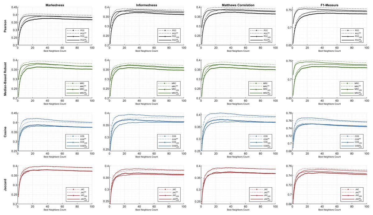
Figure 4: The evaluation over ML100K: similarity weight and preeminent metric combination to compare the dynamicity and weight significance.
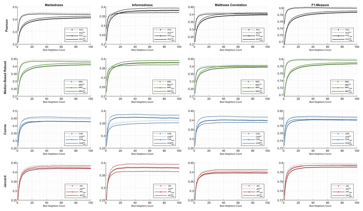
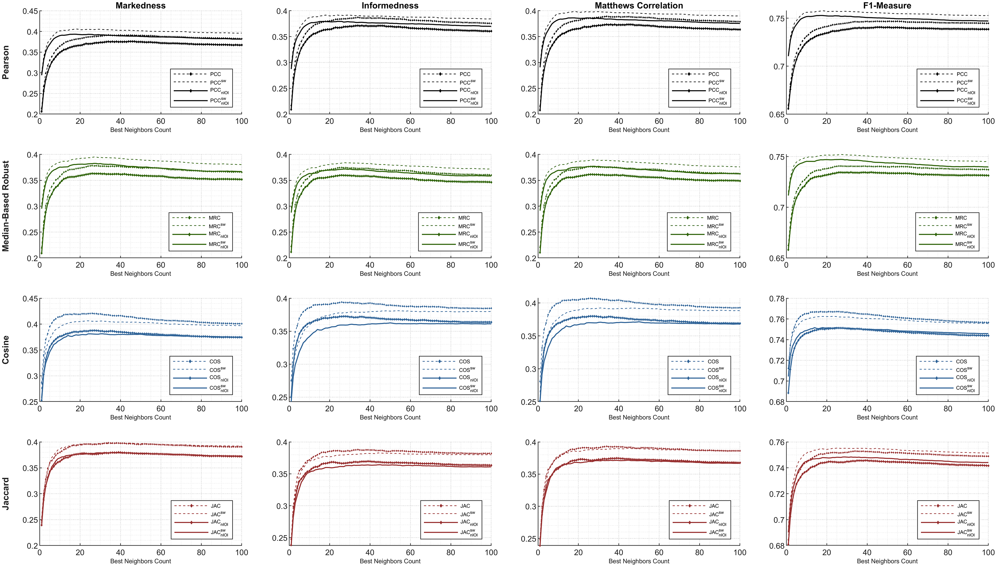
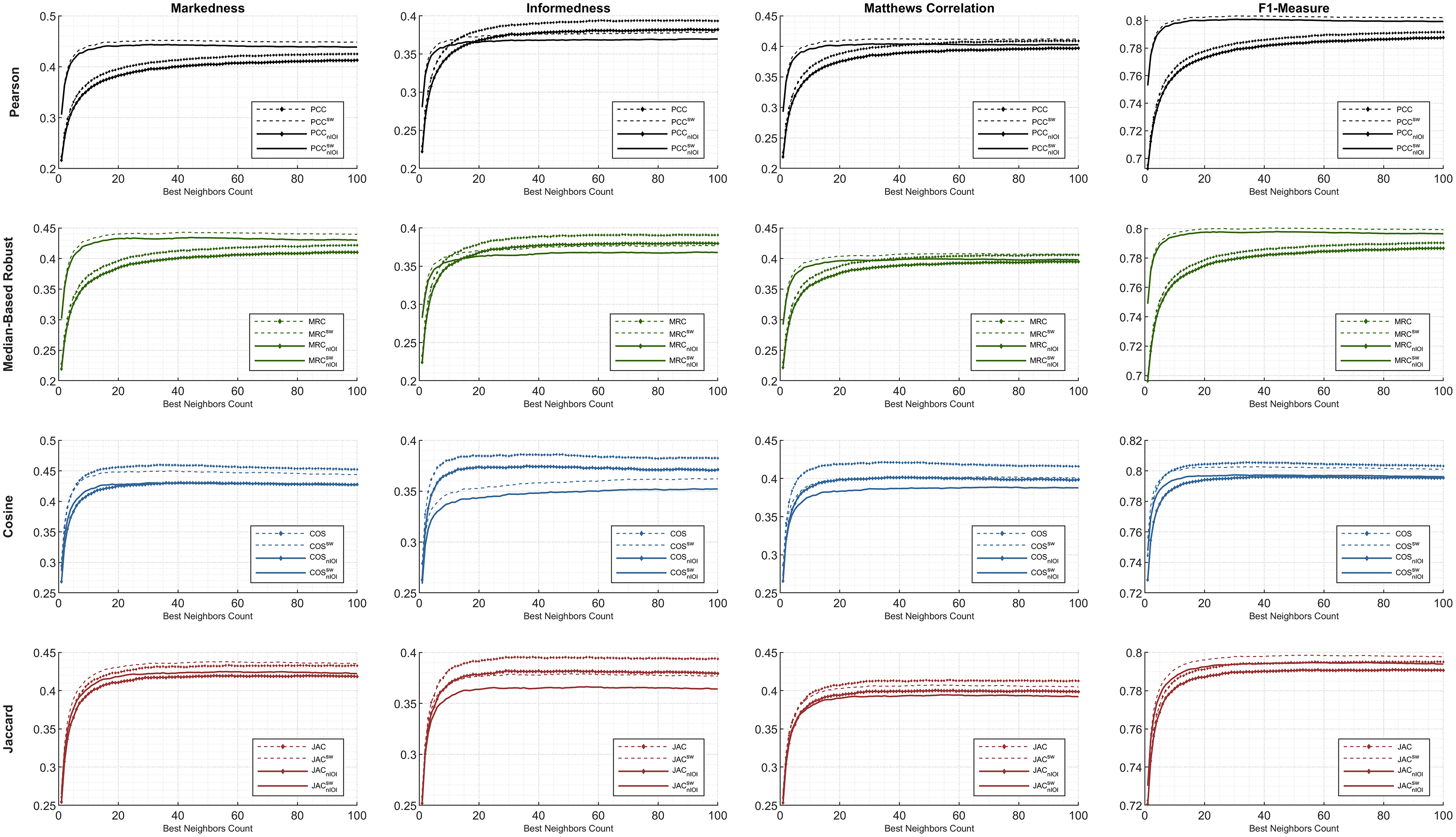
Figure 5: The evaluation over ML1M: similarity weight and preeminent metric combination to compare the dynamicity and weight significance.
Comparatively, we present the same metric performance throughout the similarity measures in the context of ML1M as shown in Fig. 5. Including only the dynamic COS, all other similarities with SW increase the F1-measure performance. However, the performance in informedness diminishes compared to that in Fig. 4. The top- and least-performing lines in each similarity measure remain the same for markedness, Matthews correlation, and F1-measure as in the ML100K. Nonetheless, regarding informedness, the effect of the SW in the PCC and MRC interchanges the least-performing similarity equation. Furthermore, dynamicity resulted in the same expected outcomes in the ML1M analysis.
B. Hybrid monitoring considering the preeminent metrics
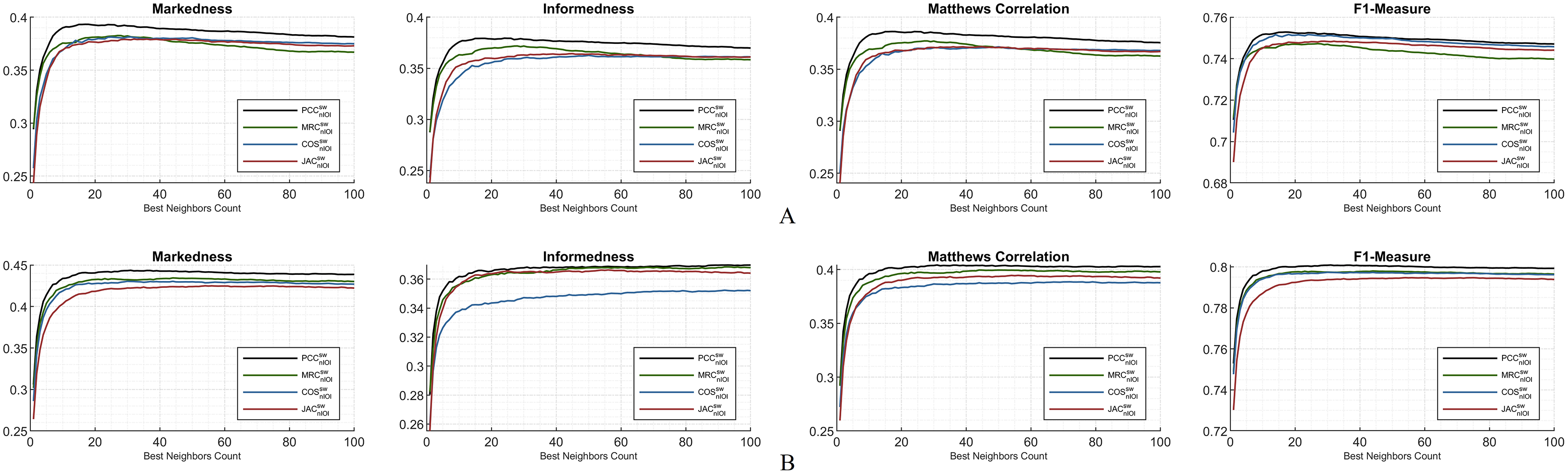
This subsection depicts the overall comparison of the compelled dynamicity with the applied weight significance. Considering Fig. 6A, for ML100K, PCC is notably in the leading position compared to other similarity measurements. The ranking for the rest of the similarity measures is difficult to generalize because the lines interchangeably depend on the BNC. Regarding markedness, MRC starts with better performance for fewer BNCs; however, the trend reverses for BNC > 27. In addition, measurements other than MRC performed better for BNC > 40. A similar behavior is valid for the informedness and Matthews correlation; nevertheless, each of them has a relatively greater BNC threshold. Approximately, BNC > 75 for informedness and BNC > 60 for Matthews correlation decayed the performance of the MRC. Considering the F1-measure, a relatively stable performance was obtained for the measurements when BNC > 10. Ranking the performance of the equations, the F1-measure can be considered as the most stable metric independent of the BNC for the ML100K. This makes it appropriate comparisons of similarity measure performances without further BNC considerations.
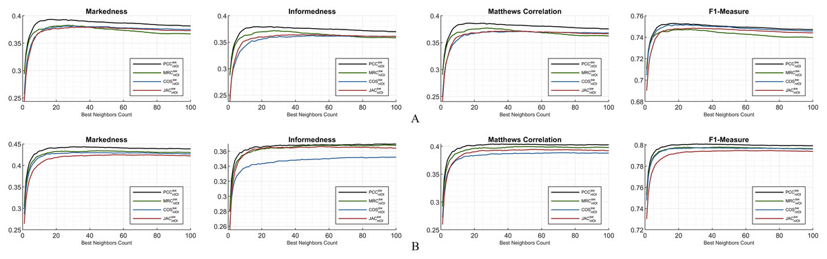
Figure 6: Markedness, informedness, and Matthews correlation as preeminent metrics, plus F1-measure highlighting the hybrid monitoring for (A) ML100K and (B) ML1M.
Regarding Fig. 6B, the same hybrid monitoring of nIOI and SW is presented for the ML1M. The top-performing lines of the abovementioned preeminent metrics were still obtained via the PCC. The COS, compared to the others, has a relatively poor performance for the informedness metric. The performance ranking of the similarity equations remains more stable as a function of the BNC compared to the ML100K. There are slight interchanges between MRC and JAC only in informedness. Nonetheless, considering the others, the relative performance is independent of the BNC. Contrary to the significant interchanges in the ML100K, performance metrics maintain their relative positions in the ML1M. This stability finding can be a general interpretation, and it can be concluded that the larger the dataset is, the more stable the performance.
C. Extensive analysis of other metrics for hybrid monitoring
The subsequent figures illustrate the extensive analysis of other metrics frequently evaluated in the literature. First, the ML100K plots with hybrid monitoring are presented in Fig. 7.
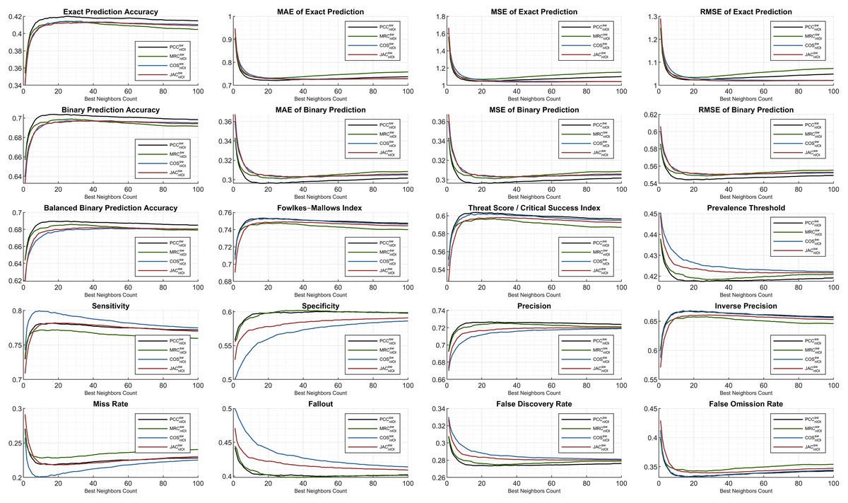
Figure 7: Extended performance evaluation on ML100K considering the hybrid monitoring.
Regarding accuracy-based metrics, both the exact (sensitive rating prediction) and binary (liked or disliked labeling) performances were monitored. The PCC had a relatively higher accuracy margin of approximately 0.05 for both metrics. Another accuracy calculation is performed extensively in this study. Considering balanced accuracy, the PCC outperformed for all the BNCs, whereas the MRC diminished. Similarly, the error metrics were measured, considering both exact and binary performances. As expected, the binary prediction error rates were lower than the exact prediction error rates. Both are plotted using MAE, MSE, and RMSE. Considering the binary prediction error, the PCC achieved the lowest possible error rates. Nonetheless, regarding the exact accuracy metric, the top performance for low error rates was interchangeable based on the neighborhood. Approximately BNC > 40, BNC > 20, and BNC > 20 for MSE, MAE, and RMSE, respectively, yielded lower error rates with the JAC measure.
In addition, the Fowlkes–Mallows index shows that PCC and COS achieve outstanding performances, whereas in general, the MRC has poor performance. Considering the threat score, the hits of user dislikes were not included; however, the ratio of liking matches concerning the misses is checked. Similarity measurement rankings are relatively stable after BNC = 10 and PCC was an adequate measure, while MRC fell behind. This implies that, after the BNC value of 10, the ranking of the metric values from similarity equations relative to the y-axis remains stable.
This study also discusses different performance checks based on the interdisciplinary applications discussed previously. Considering the context of RS, we propose the application of a prevalence threshold that sources compound information, including several associated metrics inferred as . Similar to the error metrics, the lesser the prevalence threshold value is, the more exactitude accomplished. Although higher values are obtained in the COS compared to the others, the PCC has proven its superiority with lower rates.
Some metrics, such as sensitivity and specificity, provide information on how likely the top-n items match the user’s taste or vice versa. Correctly identified positives (i.e., sensitivity) perform well for the lower BNCs, and the COS measure leads with a peak of approximately BNC = 9. Correctly identified negatives (i.e., specificity) are distinctively better as the neighbor count increases for COS and JAC, whereas PCC and MRC are relatively stable.
The last two rows of the subplots are complementary metric couples. The metrics of sensitivity and miss rate; specificity and fallout; precision and false discovery rate; inverse precision and false omission rate complete each other. Considering specificity, precision, and inverse precision, PCC performs adequately, which can be verified from fallout, false discovery rate, and false omission rate.
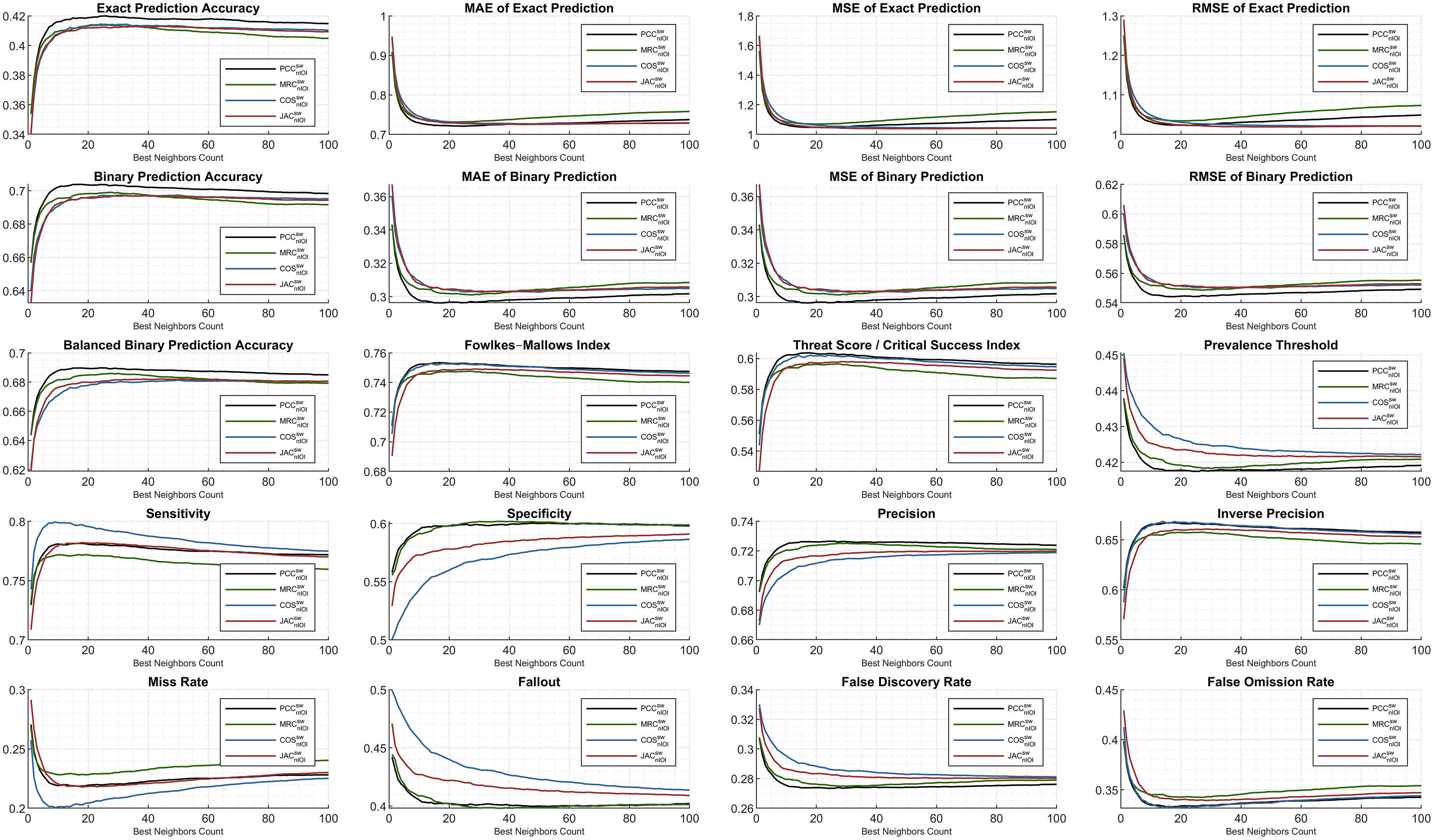
The ML1M evaluation is presented comparatively to the previous findings of the ML100K. Regarding Fig. 8, the analyses are illustrated for the same evaluated metrics. The trend in the exact accuracy was similar to that of the ML100K with greater scores. The PCC puts a margin, whereas the others perform closer to each other with slightly lower values compared to the PCC. In addition, the exact prediction error metrics generally result in a reduced numerical range. The most erroneous metric is the COS, which is valid for both exact and binary prediction error metrics. The error performance in the ML1M is relatively stable, and the PCC is still a less fragile metric for binary prediction. Considering binary analyses, similarity measures are homogenously ranked again with the dominance of the PCC.
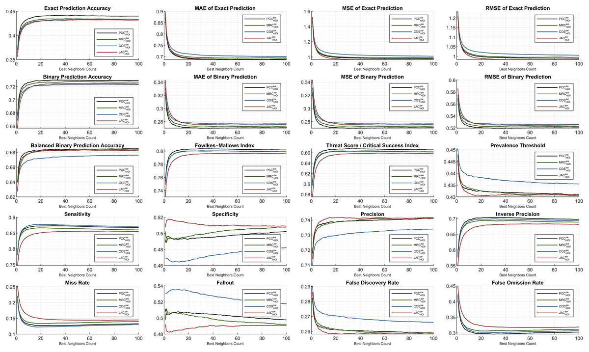
Figure 8: Extended performance evaluation on ML1M considering the hybrid monitoring.
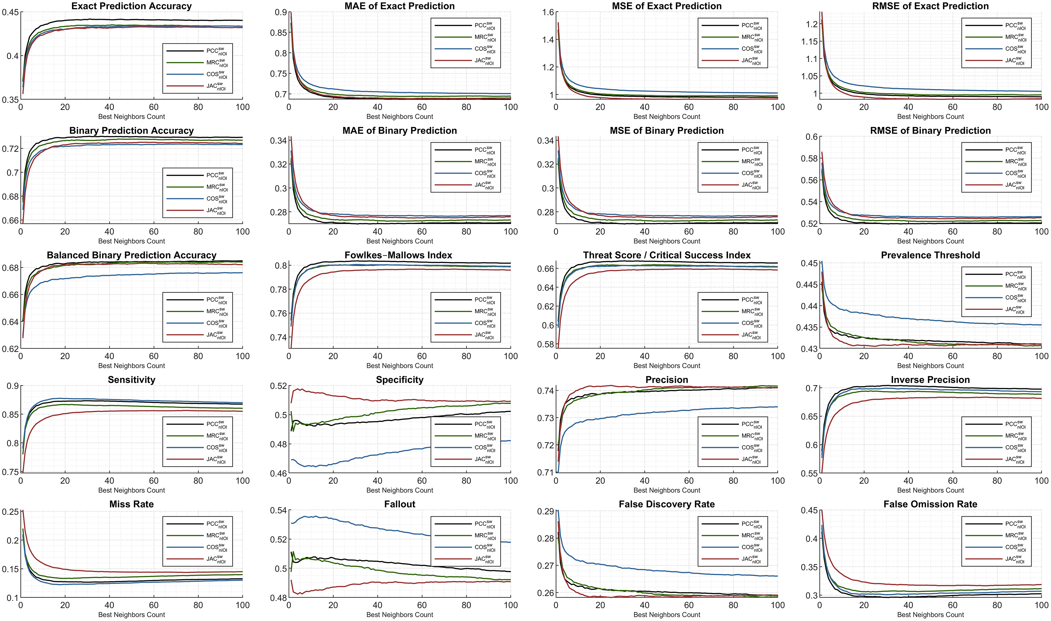
Furthermore, the Fowlkes–Mallows index shows an increased range of scoring with respect to the ML100K findings. Regarding the threat score, it was observed that the MRC significantly improved compared to the others. Considering the prevalence threshold, COS had a higher margin than the others compared to the performances in the previous analysis. Moreover, although the COS has a good sensitivity observation, it performs worse in terms of specificity and precision, as demonstrated in the previous findings. This indicates that the COS suffers from a true negative rate and positive predictive value.
The monitoring of smooth sensitivity in the ML1M is an important feedback because it is a component of some compound metrics. On the contrary, an indicative finding from the comparison of both releases is the behavior of the specificity and fallout metric couples. Considering the ML100K, a relatively more stable distribution is monitored for increasing the BNC values, whereas in the ML1M, the behavior becomes unstable. Lastly, whereas JAC for precision increases in the ranking compared to the previous findings, the opposite is valid for the inverse precision.
D. Adequate weight-metric combination of the top-performing BNCs
Having represented all the plots, we summarize the test results using a tabular structure for a compact heat-map presentation. Considering Tables 10 and 11, the performance metrics for each similarity measurement are visualized in a colored format2 . Considering the preliminarily explanations in the third section, the selected BNCs achieving the top performances are added to the tables, highlighting the main motivation of our study: the decision of adequate weight-metric combinations. Each metric is processed through column-wise coloring to make the comparison easier. Therefore, each coloring is evaluated within its own column. This indicates that the same color may correspond to different values in other columns; nevertheless, only a single column should be considered to interpret the coloring for any metric. The comparison of the similarity methods in the vertical direction is targeted, considering the neighborhoods. At the end of each heat-map table, the minimum and maximum values referenced in the coloring of the relevant column are shown. The tables demonstrate the comparison by addressing the different correlation equations over the outstanding neighborhoods; thereby, comparing approaches such as dynamicity and SW, considering each independent metric. The cells shaded in green indicate the effectiveness of the appropriate combination. We present the results using both the SW-induced dynamic equations and plain dynamicity; hence, the effect of weight boosting is monitored.
| Performance metrics | |||||||||||||||||||||||||
|---|---|---|---|---|---|---|---|---|---|---|---|---|---|---|---|---|---|---|---|---|---|---|---|---|---|
| Equation | BNC | Markedness | Informedness | Matthews correlation | F1-measure | MAE exact | MSE exact | RMSE exact | MAE threshold | MSE threshold | RMSE threshold | Accuracy exact | Accuracy threshold | Accuracy balanced | Fowlkes-Mallows index | Prevalence threshold | Threat score | Precision | Inverse precision | Sensitivity/Recall | Specificity | Fallout | Miss rate | False discovery rate | False omission rate |
| 17 | 0.364 | 0.363 | 0.364 | 0.733 | 0.744 | 1.081 | 1.040 | 0.310 | 0.310 | 0.557 | 0.403 | 0.690 | 0.681 | 0.733 | 0.416 | 0.579 | 0.729 | 0.635 | 0.737 | 0.626 | 0.374 | 0.263 | 0.271 | 0.365 | |
| 23 | 0.371 | 0.368 | 0.369 | 0.737 | 0.740 | 1.075 | 1.037 | 0.307 | 0.307 | 0.554 | 0.405 | 0.693 | 0.684 | 0.737 | 0.416 | 0.583 | 0.730 | 0.641 | 0.744 | 0.624 | 0.376 | 0.256 | 0.270 | 0.359 | |
| 34 | 0.375 | 0.371 | 0.373 | 0.740 | 0.739 | 1.078 | 1.038 | 0.304 | 0.304 | 0.552 | 0.407 | 0.696 | 0.686 | 0.740 | 0.415 | 0.587 | 0.730 | 0.645 | 0.750 | 0.622 | 0.378 | 0.250 | 0.270 | 0.355 | |
| 45 | 0.376 | 0.371 | 0.374 | 0.741 | 0.742 | 1.091 | 1.044 | 0.304 | 0.304 | 0.551 | 0.406 | 0.696 | 0.686 | 0.741 | 0.416 | 0.588 | 0.729 | 0.647 | 0.752 | 0.619 | 0.381 | 0.248 | 0.271 | 0.353 | |
| 47 | 0.376 | 0.371 | 0.373 | 0.741 | 0.742 | 1.092 | 1.045 | 0.304 | 0.304 | 0.552 | 0.406 | 0.696 | 0.685 | 0.741 | 0.416 | 0.588 | 0.729 | 0.647 | 0.753 | 0.618 | 0.382 | 0.247 | 0.271 | 0.353 | |
| 100 | 0.367 | 0.360 | 0.364 | 0.739 | 0.756 | 1.141 | 1.068 | 0.308 | 0.308 | 0.555 | 0.403 | 0.692 | 0.680 | 0.739 | 0.419 | 0.586 | 0.723 | 0.644 | 0.754 | 0.606 | 0.394 | 0.246 | 0.277 | 0.356 | |
| 17 | 0.393 | 0.379 | 0.386 | 0.753 | 0.722 | 1.048 | 1.023 | 0.296 | 0.296 | 0.544 | 0.419 | 0.704 | 0.690 | 0.753 | 0.418 | 0.604 | 0.726 | 0.667 | 0.781 | 0.598 | 0.402 | 0.219 | 0.274 | 0.333 | |
| 22 | 0.392 | 0.379 | 0.385 | 0.752 | 0.721 | 1.046 | 1.023 | 0.297 | 0.297 | 0.545 | 0.419 | 0.703 | 0.689 | 0.753 | 0.418 | 0.603 | 0.726 | 0.666 | 0.780 | 0.598 | 0.402 | 0.220 | 0.274 | 0.334 | |
| 24 | 0.393 | 0.379 | 0.386 | 0.753 | 0.721 | 1.047 | 1.023 | 0.296 | 0.296 | 0.544 | 0.420 | 0.704 | 0.690 | 0.753 | 0.417 | 0.603 | 0.727 | 0.666 | 0.780 | 0.599 | 0.401 | 0.220 | 0.273 | 0.334 | |
| 26 | 0.393 | 0.379 | 0.386 | 0.752 | 0.721 | 1.049 | 1.024 | 0.296 | 0.296 | 0.544 | 0.420 | 0.704 | 0.690 | 0.753 | 0.417 | 0.603 | 0.727 | 0.666 | 0.780 | 0.599 | 0.401 | 0.220 | 0.273 | 0.334 | |
| 53 | 0.388 | 0.376 | 0.382 | 0.750 | 0.728 | 1.070 | 1.034 | 0.299 | 0.299 | 0.547 | 0.418 | 0.701 | 0.688 | 0.750 | 0.418 | 0.600 | 0.726 | 0.662 | 0.775 | 0.600 | 0.400 | 0.225 | 0.274 | 0.338 | |
| 12 | 0.353 | 0.351 | 0.352 | 0.728 | 0.755 | 1.105 | 1.051 | 0.316 | 0.316 | 0.562 | 0.397 | 0.684 | 0.676 | 0.728 | 0.419 | 0.572 | 0.724 | 0.628 | 0.732 | 0.620 | 0.380 | 0.268 | 0.276 | 0.372 | |
| 19 | 0.358 | 0.356 | 0.357 | 0.732 | 0.750 | 1.096 | 1.047 | 0.313 | 0.313 | 0.559 | 0.400 | 0.687 | 0.678 | 0.732 | 0.419 | 0.577 | 0.725 | 0.634 | 0.738 | 0.617 | 0.383 | 0.262 | 0.275 | 0.366 | |
| 25 | 0.363 | 0.360 | 0.361 | 0.734 | 0.748 | 1.098 | 1.048 | 0.311 | 0.311 | 0.557 | 0.402 | 0.689 | 0.680 | 0.734 | 0.418 | 0.580 | 0.726 | 0.637 | 0.743 | 0.617 | 0.383 | 0.257 | 0.274 | 0.363 | |
| 26 | 0.363 | 0.360 | 0.361 | 0.734 | 0.748 | 1.099 | 1.048 | 0.310 | 0.310 | 0.557 | 0.402 | 0.690 | 0.680 | 0.734 | 0.418 | 0.580 | 0.726 | 0.637 | 0.743 | 0.617 | 0.383 | 0.257 | 0.274 | 0.363 | |
| 27 | 0.363 | 0.360 | 0.361 | 0.734 | 0.748 | 1.099 | 1.048 | 0.310 | 0.310 | 0.557 | 0.402 | 0.690 | 0.680 | 0.734 | 0.418 | 0.580 | 0.726 | 0.638 | 0.744 | 0.616 | 0.384 | 0.256 | 0.274 | 0.362 | |
| 42 | 0.362 | 0.358 | 0.360 | 0.735 | 0.754 | 1.121 | 1.058 | 0.311 | 0.311 | 0.557 | 0.401 | 0.689 | 0.679 | 0.735 | 0.419 | 0.581 | 0.724 | 0.638 | 0.745 | 0.613 | 0.387 | 0.255 | 0.276 | 0.362 | |
| 59 | 0.358 | 0.353 | 0.356 | 0.734 | 0.761 | 1.147 | 1.071 | 0.313 | 0.313 | 0.559 | 0.400 | 0.687 | 0.677 | 0.734 | 0.420 | 0.579 | 0.722 | 0.636 | 0.746 | 0.607 | 0.393 | 0.254 | 0.278 | 0.364 | |
| 17 | 0.380 | 0.369 | 0.375 | 0.747 | 0.733 | 1.071 | 1.035 | 0.302 | 0.302 | 0.550 | 0.412 | 0.698 | 0.684 | 0.747 | 0.419 | 0.596 | 0.723 | 0.657 | 0.772 | 0.597 | 0.403 | 0.228 | 0.277 | 0.343 | |
| 20 | 0.381 | 0.370 | 0.375 | 0.747 | 0.732 | 1.069 | 1.034 | 0.302 | 0.302 | 0.549 | 0.413 | 0.698 | 0.685 | 0.747 | 0.419 | 0.596 | 0.724 | 0.657 | 0.772 | 0.598 | 0.402 | 0.228 | 0.276 | 0.343 | |
| 23 | 0.381 | 0.370 | 0.376 | 0.747 | 0.731 | 1.070 | 1.035 | 0.302 | 0.302 | 0.549 | 0.414 | 0.698 | 0.685 | 0.747 | 0.419 | 0.596 | 0.724 | 0.657 | 0.771 | 0.599 | 0.401 | 0.229 | 0.276 | 0.343 | |
| 27 | 0.383 | 0.372 | 0.377 | 0.747 | 0.732 | 1.072 | 1.035 | 0.301 | 0.301 | 0.549 | 0.414 | 0.699 | 0.686 | 0.748 | 0.418 | 0.597 | 0.725 | 0.658 | 0.771 | 0.601 | 0.399 | 0.229 | 0.275 | 0.342 | |
| 28 | 0.383 | 0.372 | 0.377 | 0.747 | 0.732 | 1.073 | 1.036 | 0.301 | 0.301 | 0.549 | 0.414 | 0.699 | 0.686 | 0.747 | 0.418 | 0.596 | 0.725 | 0.657 | 0.770 | 0.601 | 0.399 | 0.230 | 0.275 | 0.343 | |
| 30 | 0.382 | 0.372 | 0.377 | 0.747 | 0.733 | 1.077 | 1.038 | 0.301 | 0.301 | 0.549 | 0.414 | 0.699 | 0.686 | 0.747 | 0.418 | 0.596 | 0.725 | 0.657 | 0.770 | 0.602 | 0.398 | 0.230 | 0.275 | 0.343 | |
| 37 | 0.380 | 0.370 | 0.375 | 0.746 | 0.736 | 1.085 | 1.042 | 0.302 | 0.302 | 0.550 | 0.413 | 0.698 | 0.685 | 0.746 | 0.419 | 0.595 | 0.725 | 0.656 | 0.768 | 0.602 | 0.398 | 0.232 | 0.275 | 0.344 | |
| 25 | 0.388 | 0.372 | 0.380 | 0.751 | 0.720 | 1.027 | 1.013 | 0.299 | 0.299 | 0.547 | 0.416 | 0.701 | 0.686 | 0.752 | 0.420 | 0.602 | 0.723 | 0.665 | 0.782 | 0.590 | 0.410 | 0.218 | 0.277 | 0.335 | |
| 27 | 0.388 | 0.373 | 0.380 | 0.751 | 0.719 | 1.025 | 1.012 | 0.299 | 0.299 | 0.547 | 0.416 | 0.701 | 0.686 | 0.752 | 0.420 | 0.602 | 0.723 | 0.665 | 0.782 | 0.591 | 0.409 | 0.218 | 0.277 | 0.335 | |
| 28 | 0.388 | 0.372 | 0.380 | 0.751 | 0.719 | 1.025 | 1.012 | 0.299 | 0.299 | 0.547 | 0.416 | 0.701 | 0.686 | 0.752 | 0.420 | 0.602 | 0.723 | 0.665 | 0.782 | 0.591 | 0.409 | 0.218 | 0.277 | 0.335 | |
| 35 | 0.387 | 0.372 | 0.379 | 0.751 | 0.720 | 1.024 | 1.012 | 0.299 | 0.299 | 0.547 | 0.415 | 0.701 | 0.686 | 0.751 | 0.420 | 0.601 | 0.723 | 0.664 | 0.781 | 0.591 | 0.409 | 0.219 | 0.277 | 0.336 | |
| 36 | 0.386 | 0.372 | 0.379 | 0.750 | 0.720 | 1.025 | 1.012 | 0.299 | 0.299 | 0.547 | 0.415 | 0.701 | 0.686 | 0.751 | 0.420 | 0.601 | 0.723 | 0.663 | 0.780 | 0.592 | 0.408 | 0.220 | 0.277 | 0.337 | |
| 100 | 0.374 | 0.364 | 0.369 | 0.744 | 0.727 | 1.035 | 1.017 | 0.305 | 0.305 | 0.552 | 0.409 | 0.695 | 0.682 | 0.744 | 0.420 | 0.592 | 0.722 | 0.652 | 0.767 | 0.597 | 0.403 | 0.233 | 0.278 | 0.348 | |
| 9 | 0.367 | 0.339 | 0.353 | 0.748 | 0.749 | 1.108 | 1.053 | 0.310 | 0.310 | 0.557 | 0.407 | 0.690 | 0.670 | 0.750 | 0.431 | 0.598 | 0.703 | 0.663 | 0.799 | 0.540 | 0.460 | 0.201 | 0.297 | 0.337 | |
| 14 | 0.378 | 0.353 | 0.365 | 0.752 | 0.736 | 1.076 | 1.037 | 0.305 | 0.305 | 0.552 | 0.412 | 0.695 | 0.676 | 0.753 | 0.428 | 0.602 | 0.710 | 0.668 | 0.799 | 0.554 | 0.446 | 0.201 | 0.290 | 0.332 | |
| 18 | 0.379 | 0.355 | 0.367 | 0.752 | 0.733 | 1.066 | 1.032 | 0.304 | 0.304 | 0.551 | 0.413 | 0.696 | 0.677 | 0.753 | 0.427 | 0.602 | 0.711 | 0.668 | 0.797 | 0.558 | 0.442 | 0.203 | 0.289 | 0.332 | |
| 24 | 0.381 | 0.359 | 0.370 | 0.752 | 0.729 | 1.056 | 1.028 | 0.303 | 0.303 | 0.550 | 0.414 | 0.697 | 0.679 | 0.753 | 0.425 | 0.602 | 0.714 | 0.668 | 0.794 | 0.565 | 0.435 | 0.206 | 0.286 | 0.332 | |
| 31 | 0.381 | 0.361 | 0.371 | 0.751 | 0.728 | 1.052 | 1.026 | 0.303 | 0.303 | 0.550 | 0.414 | 0.697 | 0.680 | 0.752 | 0.425 | 0.602 | 0.715 | 0.666 | 0.791 | 0.569 | 0.431 | 0.209 | 0.285 | 0.334 | |
| 50 | 0.381 | 0.363 | 0.371 | 0.750 | 0.726 | 1.045 | 1.022 | 0.303 | 0.303 | 0.550 | 0.413 | 0.697 | 0.681 | 0.751 | 0.423 | 0.600 | 0.717 | 0.663 | 0.785 | 0.577 | 0.423 | 0.215 | 0.283 | 0.337 | |
| 67 | 0.377 | 0.361 | 0.369 | 0.748 | 0.727 | 1.043 | 1.021 | 0.304 | 0.304 | 0.551 | 0.412 | 0.696 | 0.681 | 0.748 | 0.423 | 0.597 | 0.718 | 0.659 | 0.780 | 0.581 | 0.419 | 0.220 | 0.282 | 0.341 | |
| 99 | 0.375 | 0.361 | 0.368 | 0.746 | 0.728 | 1.044 | 1.022 | 0.305 | 0.305 | 0.552 | 0.410 | 0.695 | 0.681 | 0.746 | 0.422 | 0.595 | 0.719 | 0.656 | 0.775 | 0.586 | 0.414 | 0.225 | 0.281 | 0.344 | |
| 100 | 0.375 | 0.361 | 0.368 | 0.746 | 0.728 | 1.044 | 1.022 | 0.305 | 0.305 | 0.552 | 0.410 | 0.695 | 0.681 | 0.746 | 0.422 | 0.595 | 0.719 | 0.656 | 0.775 | 0.586 | 0.414 | 0.225 | 0.281 | 0.344 | |
| 20 | 0.377 | 0.368 | 0.373 | 0.744 | 0.727 | 1.034 | 1.017 | 0.303 | 0.303 | 0.551 | 0.409 | 0.697 | 0.684 | 0.745 | 0.419 | 0.593 | 0.724 | 0.653 | 0.766 | 0.602 | 0.398 | 0.234 | 0.276 | 0.347 | |
| 35 | 0.379 | 0.369 | 0.374 | 0.746 | 0.724 | 1.026 | 1.013 | 0.303 | 0.303 | 0.550 | 0.410 | 0.697 | 0.684 | 0.746 | 0.419 | 0.594 | 0.724 | 0.655 | 0.768 | 0.601 | 0.399 | 0.232 | 0.276 | 0.345 | |
| 36 | 0.380 | 0.369 | 0.374 | 0.746 | 0.724 | 1.026 | 1.013 | 0.302 | 0.302 | 0.550 | 0.411 | 0.698 | 0.685 | 0.746 | 0.419 | 0.594 | 0.724 | 0.655 | 0.768 | 0.601 | 0.399 | 0.232 | 0.276 | 0.345 | |
| 39 | 0.380 | 0.370 | 0.375 | 0.746 | 0.723 | 1.025 | 1.012 | 0.302 | 0.302 | 0.550 | 0.410 | 0.698 | 0.685 | 0.746 | 0.419 | 0.595 | 0.725 | 0.655 | 0.768 | 0.602 | 0.398 | 0.232 | 0.275 | 0.345 | |
| 40 | 0.380 | 0.370 | 0.375 | 0.746 | 0.723 | 1.025 | 1.012 | 0.302 | 0.302 | 0.550 | 0.410 | 0.698 | 0.685 | 0.746 | 0.419 | 0.595 | 0.725 | 0.655 | 0.768 | 0.601 | 0.399 | 0.232 | 0.275 | 0.345 | |
| 18 | 0.377 | 0.360 | 0.368 | 0.748 | 0.729 | 1.050 | 1.025 | 0.304 | 0.304 | 0.552 | 0.412 | 0.696 | 0.680 | 0.749 | 0.424 | 0.597 | 0.717 | 0.660 | 0.782 | 0.578 | 0.422 | 0.218 | 0.283 | 0.340 | |
| 29 | 0.379 | 0.363 | 0.371 | 0.748 | 0.726 | 1.042 | 1.021 | 0.303 | 0.303 | 0.551 | 0.412 | 0.697 | 0.681 | 0.749 | 0.422 | 0.598 | 0.718 | 0.661 | 0.781 | 0.582 | 0.418 | 0.219 | 0.282 | 0.339 | |
| 32 | 0.379 | 0.364 | 0.371 | 0.748 | 0.726 | 1.041 | 1.020 | 0.303 | 0.303 | 0.550 | 0.413 | 0.697 | 0.682 | 0.749 | 0.422 | 0.598 | 0.719 | 0.661 | 0.781 | 0.583 | 0.417 | 0.219 | 0.281 | 0.339 | |
| 36 | 0.379 | 0.364 | 0.372 | 0.748 | 0.725 | 1.039 | 1.020 | 0.303 | 0.303 | 0.550 | 0.413 | 0.697 | 0.682 | 0.749 | 0.422 | 0.598 | 0.719 | 0.660 | 0.780 | 0.584 | 0.416 | 0.220 | 0.281 | 0.340 | |
| 44 | 0.379 | 0.364 | 0.372 | 0.748 | 0.725 | 1.038 | 1.019 | 0.303 | 0.303 | 0.550 | 0.413 | 0.697 | 0.682 | 0.748 | 0.422 | 0.597 | 0.720 | 0.660 | 0.779 | 0.586 | 0.414 | 0.221 | 0.280 | 0.340 | |
| 45 | 0.379 | 0.364 | 0.372 | 0.748 | 0.725 | 1.038 | 1.019 | 0.303 | 0.303 | 0.550 | 0.413 | 0.697 | 0.682 | 0.748 | 0.422 | 0.597 | 0.720 | 0.659 | 0.778 | 0.586 | 0.414 | 0.222 | 0.280 | 0.341 | |
| 59 | 0.377 | 0.363 | 0.370 | 0.747 | 0.726 | 1.038 | 1.019 | 0.304 | 0.304 | 0.551 | 0.412 | 0.696 | 0.682 | 0.747 | 0.422 | 0.596 | 0.720 | 0.657 | 0.775 | 0.588 | 0.412 | 0.225 | 0.280 | 0.343 | |
| 100 | 0.373 | 0.361 | 0.367 | 0.744 | 0.729 | 1.042 | 1.021 | 0.306 | 0.306 | 0.553 | 0.409 | 0.694 | 0.681 | 0.745 | 0.422 | 0.593 | 0.720 | 0.653 | 0.770 | 0.591 | 0.409 | 0.230 | 0.280 | 0.347 | |
| min | 0.353 | 0.339 | 0.352 | 0.728 | 0.719 | 1.024 | 1.012 | 0.296 | 0.296 | 0.544 | 0.397 | 0.684 | 0.670 | 0.728 | 0.415 | 0.572 | 0.703 | 0.628 | 0.732 | 0.540 | 0.374 | 0.201 | 0.270 | 0.332 | |
| max | 0.393 | 0.379 | 0.386 | 0.753 | 0.761 | 1.147 | 1.071 | 0.316 | 0.316 | 0.562 | 0.420 | 0.704 | 0.690 | 0.753 | 0.431 | 0.604 | 0.730 | 0.668 | 0.799 | 0.626 | 0.460 | 0.268 | 0.297 | 0.372 | |
Note:
The fractional values in the table are displayed based on three significant digits. The heat-map coloring is achieved according to full precision.
| Performance metrics | |||||||||||||||||||||||||
|---|---|---|---|---|---|---|---|---|---|---|---|---|---|---|---|---|---|---|---|---|---|---|---|---|---|
| Equation | BNC | Markedness | Informedness | Matthews correlation | F1-measure | MAE exact | MSE exact | RMSE exact | MAE threshold | MSE threshold | RMSE threshold | Accuracy exact | Accuracy threshold | Accuracy balanced | Fowlkes-Mallows index | Prevalence threshold | Threat score | Precision | Inverse precision | Sensitivity/Recall | Specificity | Fallout | Miss rate | False discovery rate | False omission rate |
| 4 | 0.305 | 0.308 | 0.307 | 0.735 | 0.797 | 1.200 | 1.096 | 0.328 | 0.328 | 0.572 | 0.378 | 0.672 | 0.654 | 0.735 | 0.432 | 0.581 | 0.740 | 0.566 | 0.730 | 0.578 | 0.422 | 0.270 | 0.260 | 0.434 | |
| 31 | 0.396 | 0.376 | 0.386 | 0.779 | 0.707 | 0.981 | 0.991 | 0.283 | 0.283 | 0.532 | 0.415 | 0.717 | 0.688 | 0.780 | 0.422 | 0.639 | 0.755 | 0.641 | 0.805 | 0.571 | 0.429 | 0.195 | 0.245 | 0.359 | |
| 91 | 0.413 | 0.382 | 0.397 | 0.787 | 0.696 | 0.966 | 0.983 | 0.277 | 0.277 | 0.526 | 0.422 | 0.723 | 0.691 | 0.788 | 0.423 | 0.649 | 0.754 | 0.659 | 0.824 | 0.559 | 0.441 | 0.176 | 0.246 | 0.341 | |
| 96 | 0.412 | 0.382 | 0.397 | 0.787 | 0.696 | 0.966 | 0.983 | 0.277 | 0.277 | 0.526 | 0.423 | 0.723 | 0.691 | 0.788 | 0.423 | 0.649 | 0.754 | 0.659 | 0.824 | 0.557 | 0.443 | 0.176 | 0.246 | 0.341 | |
| 99 | 0.413 | 0.382 | 0.397 | 0.787 | 0.696 | 0.966 | 0.983 | 0.277 | 0.277 | 0.526 | 0.422 | 0.723 | 0.691 | 0.788 | 0.423 | 0.649 | 0.754 | 0.659 | 0.825 | 0.557 | 0.443 | 0.175 | 0.246 | 0.341 | |
| 100 | 0.413 | 0.382 | 0.397 | 0.788 | 0.696 | 0.966 | 0.983 | 0.277 | 0.277 | 0.526 | 0.423 | 0.723 | 0.691 | 0.788 | 0.423 | 0.650 | 0.754 | 0.659 | 0.825 | 0.557 | 0.443 | 0.175 | 0.246 | 0.341 | |
| 31 | 0.444 | 0.368 | 0.404 | 0.801 | 0.688 | 0.988 | 0.994 | 0.270 | 0.270 | 0.520 | 0.442 | 0.730 | 0.684 | 0.804 | 0.432 | 0.668 | 0.740 | 0.704 | 0.873 | 0.495 | 0.505 | 0.127 | 0.260 | 0.296 | |
| 93 | 0.439 | 0.370 | 0.403 | 0.799 | 0.687 | 0.981 | 0.990 | 0.271 | 0.271 | 0.520 | 0.440 | 0.729 | 0.685 | 0.802 | 0.431 | 0.666 | 0.741 | 0.698 | 0.868 | 0.502 | 0.498 | 0.132 | 0.259 | 0.302 | |
| 100 | 0.439 | 0.370 | 0.403 | 0.799 | 0.687 | 0.979 | 0.990 | 0.271 | 0.271 | 0.520 | 0.440 | 0.729 | 0.685 | 0.802 | 0.431 | 0.666 | 0.741 | 0.698 | 0.867 | 0.502 | 0.498 | 0.133 | 0.259 | 0.302 | |
| 8 | 0.351 | 0.344 | 0.347 | 0.759 | 0.747 | 1.075 | 1.037 | 0.304 | 0.304 | 0.552 | 0.398 | 0.696 | 0.672 | 0.759 | 0.426 | 0.611 | 0.748 | 0.603 | 0.769 | 0.575 | 0.425 | 0.231 | 0.252 | 0.397 | |
| 48 | 0.403 | 0.379 | 0.391 | 0.783 | 0.704 | 0.980 | 0.990 | 0.280 | 0.280 | 0.530 | 0.417 | 0.720 | 0.689 | 0.784 | 0.422 | 0.643 | 0.754 | 0.649 | 0.814 | 0.564 | 0.436 | 0.186 | 0.246 | 0.351 | |
| 60 | 0.406 | 0.379 | 0.393 | 0.785 | 0.702 | 0.978 | 0.989 | 0.279 | 0.279 | 0.528 | 0.419 | 0.721 | 0.690 | 0.785 | 0.423 | 0.646 | 0.754 | 0.652 | 0.818 | 0.562 | 0.438 | 0.182 | 0.246 | 0.348 | |
| 92 | 0.411 | 0.380 | 0.395 | 0.787 | 0.701 | 0.980 | 0.990 | 0.278 | 0.278 | 0.527 | 0.421 | 0.722 | 0.690 | 0.787 | 0.423 | 0.648 | 0.753 | 0.657 | 0.823 | 0.557 | 0.443 | 0.177 | 0.247 | 0.343 | |
| 97 | 0.411 | 0.380 | 0.395 | 0.787 | 0.701 | 0.979 | 0.990 | 0.278 | 0.278 | 0.527 | 0.420 | 0.722 | 0.690 | 0.787 | 0.423 | 0.648 | 0.753 | 0.657 | 0.823 | 0.557 | 0.443 | 0.177 | 0.247 | 0.343 | |
| 100 | 0.410 | 0.380 | 0.395 | 0.787 | 0.701 | 0.980 | 0.990 | 0.278 | 0.278 | 0.527 | 0.420 | 0.722 | 0.690 | 0.787 | 0.423 | 0.648 | 0.753 | 0.657 | 0.823 | 0.556 | 0.444 | 0.177 | 0.247 | 0.343 | |
| 23 | 0.434 | 0.364 | 0.397 | 0.798 | 0.698 | 1.001 | 1.001 | 0.273 | 0.273 | 0.523 | 0.434 | 0.727 | 0.682 | 0.800 | 0.432 | 0.664 | 0.739 | 0.695 | 0.867 | 0.497 | 0.503 | 0.133 | 0.261 | 0.305 | |
| 41 | 0.434 | 0.366 | 0.399 | 0.798 | 0.694 | 0.992 | 0.996 | 0.273 | 0.273 | 0.522 | 0.435 | 0.727 | 0.683 | 0.800 | 0.432 | 0.664 | 0.740 | 0.693 | 0.865 | 0.501 | 0.499 | 0.135 | 0.260 | 0.307 | |
| 44 | 0.434 | 0.367 | 0.400 | 0.798 | 0.694 | 0.992 | 0.996 | 0.272 | 0.272 | 0.522 | 0.435 | 0.728 | 0.684 | 0.800 | 0.431 | 0.664 | 0.741 | 0.694 | 0.865 | 0.502 | 0.498 | 0.135 | 0.259 | 0.306 | |
| 58 | 0.433 | 0.368 | 0.399 | 0.798 | 0.694 | 0.990 | 0.995 | 0.272 | 0.272 | 0.522 | 0.435 | 0.728 | 0.684 | 0.800 | 0.431 | 0.663 | 0.741 | 0.692 | 0.863 | 0.505 | 0.495 | 0.137 | 0.259 | 0.308 | |
| 93 | 0.431 | 0.368 | 0.398 | 0.797 | 0.694 | 0.989 | 0.995 | 0.273 | 0.273 | 0.522 | 0.434 | 0.727 | 0.684 | 0.799 | 0.431 | 0.662 | 0.742 | 0.689 | 0.861 | 0.508 | 0.492 | 0.139 | 0.258 | 0.311 | |
| 94 | 0.431 | 0.368 | 0.398 | 0.797 | 0.694 | 0.989 | 0.995 | 0.273 | 0.273 | 0.522 | 0.434 | 0.727 | 0.684 | 0.799 | 0.431 | 0.662 | 0.742 | 0.689 | 0.861 | 0.508 | 0.492 | 0.139 | 0.258 | 0.311 | |
| 96 | 0.431 | 0.368 | 0.398 | 0.797 | 0.694 | 0.990 | 0.995 | 0.273 | 0.273 | 0.522 | 0.434 | 0.727 | 0.684 | 0.799 | 0.431 | 0.662 | 0.742 | 0.689 | 0.860 | 0.508 | 0.492 | 0.140 | 0.258 | 0.311 | |
| 4 | 0.373 | 0.346 | 0.359 | 0.774 | 0.736 | 1.070 | 1.034 | 0.294 | 0.294 | 0.542 | 0.410 | 0.706 | 0.673 | 0.775 | 0.431 | 0.631 | 0.742 | 0.631 | 0.809 | 0.537 | 0.463 | 0.191 | 0.258 | 0.369 | |
| 13 | 0.418 | 0.372 | 0.394 | 0.792 | 0.692 | 0.969 | 0.984 | 0.276 | 0.276 | 0.525 | 0.430 | 0.724 | 0.686 | 0.793 | 0.428 | 0.655 | 0.746 | 0.673 | 0.843 | 0.528 | 0.472 | 0.157 | 0.254 | 0.327 | |
| 36 | 0.430 | 0.375 | 0.402 | 0.796 | 0.684 | 0.951 | 0.975 | 0.272 | 0.272 | 0.522 | 0.434 | 0.728 | 0.687 | 0.798 | 0.428 | 0.661 | 0.745 | 0.685 | 0.854 | 0.520 | 0.480 | 0.146 | 0.255 | 0.315 | |
| 41 | 0.431 | 0.374 | 0.402 | 0.796 | 0.683 | 0.950 | 0.975 | 0.272 | 0.272 | 0.522 | 0.434 | 0.728 | 0.687 | 0.798 | 0.428 | 0.661 | 0.745 | 0.686 | 0.855 | 0.520 | 0.480 | 0.145 | 0.255 | 0.314 | |
| 45 | 0.430 | 0.374 | 0.401 | 0.796 | 0.683 | 0.949 | 0.974 | 0.272 | 0.272 | 0.522 | 0.434 | 0.728 | 0.687 | 0.798 | 0.429 | 0.661 | 0.745 | 0.685 | 0.855 | 0.519 | 0.481 | 0.145 | 0.255 | 0.315 | |
| 50 | 0.430 | 0.374 | 0.401 | 0.796 | 0.683 | 0.951 | 0.975 | 0.272 | 0.272 | 0.522 | 0.434 | 0.728 | 0.687 | 0.798 | 0.429 | 0.661 | 0.745 | 0.686 | 0.855 | 0.518 | 0.482 | 0.145 | 0.255 | 0.314 | |
| 72 | 0.429 | 0.372 | 0.399 | 0.796 | 0.684 | 0.954 | 0.977 | 0.273 | 0.273 | 0.522 | 0.435 | 0.727 | 0.686 | 0.798 | 0.429 | 0.661 | 0.744 | 0.685 | 0.855 | 0.517 | 0.483 | 0.145 | 0.256 | 0.315 | |
| 83 | 0.429 | 0.371 | 0.399 | 0.796 | 0.684 | 0.954 | 0.977 | 0.273 | 0.273 | 0.523 | 0.434 | 0.727 | 0.686 | 0.798 | 0.429 | 0.661 | 0.744 | 0.685 | 0.855 | 0.516 | 0.484 | 0.145 | 0.256 | 0.315 | |
| 18 | 0.428 | 0.343 | 0.383 | 0.797 | 0.712 | 1.044 | 1.022 | 0.278 | 0.278 | 0.527 | 0.430 | 0.722 | 0.672 | 0.800 | 0.438 | 0.662 | 0.730 | 0.699 | 0.878 | 0.466 | 0.534 | 0.122 | 0.270 | 0.301 | |
| 30 | 0.430 | 0.347 | 0.387 | 0.797 | 0.706 | 1.030 | 1.015 | 0.277 | 0.277 | 0.526 | 0.433 | 0.723 | 0.674 | 0.801 | 0.437 | 0.663 | 0.731 | 0.699 | 0.877 | 0.470 | 0.530 | 0.123 | 0.269 | 0.301 | |
| 72 | 0.429 | 0.352 | 0.389 | 0.797 | 0.701 | 1.015 | 1.007 | 0.276 | 0.276 | 0.526 | 0.434 | 0.724 | 0.676 | 0.800 | 0.436 | 0.662 | 0.733 | 0.696 | 0.873 | 0.479 | 0.521 | 0.127 | 0.267 | 0.304 | |
| 91 | 0.428 | 0.352 | 0.388 | 0.796 | 0.701 | 1.012 | 1.006 | 0.277 | 0.277 | 0.526 | 0.434 | 0.723 | 0.676 | 0.799 | 0.436 | 0.662 | 0.734 | 0.694 | 0.871 | 0.481 | 0.519 | 0.129 | 0.266 | 0.306 | |
| 92 | 0.428 | 0.352 | 0.388 | 0.796 | 0.701 | 1.012 | 1.006 | 0.277 | 0.277 | 0.526 | 0.434 | 0.723 | 0.676 | 0.799 | 0.436 | 0.662 | 0.734 | 0.694 | 0.871 | 0.482 | 0.518 | 0.129 | 0.266 | 0.306 | |
| 97 | 0.427 | 0.352 | 0.388 | 0.796 | 0.701 | 1.011 | 1.006 | 0.277 | 0.277 | 0.526 | 0.434 | 0.723 | 0.676 | 0.799 | 0.436 | 0.661 | 0.734 | 0.693 | 0.870 | 0.482 | 0.518 | 0.130 | 0.266 | 0.307 | |
| 99 | 0.427 | 0.352 | 0.388 | 0.796 | 0.701 | 1.011 | 1.005 | 0.277 | 0.277 | 0.526 | 0.433 | 0.723 | 0.676 | 0.799 | 0.435 | 0.661 | 0.734 | 0.693 | 0.870 | 0.482 | 0.518 | 0.130 | 0.266 | 0.307 | |
| 100 | 0.427 | 0.352 | 0.388 | 0.796 | 0.701 | 1.011 | 1.005 | 0.277 | 0.277 | 0.526 | 0.433 | 0.723 | 0.676 | 0.799 | 0.436 | 0.661 | 0.734 | 0.693 | 0.870 | 0.482 | 0.518 | 0.130 | 0.266 | 0.307 | |
| 10 | 0.396 | 0.369 | 0.382 | 0.781 | 0.705 | 0.983 | 0.991 | 0.284 | 0.284 | 0.533 | 0.419 | 0.716 | 0.685 | 0.782 | 0.425 | 0.641 | 0.750 | 0.646 | 0.814 | 0.555 | 0.445 | 0.186 | 0.250 | 0.354 | |
| 29 | 0.417 | 0.382 | 0.399 | 0.790 | 0.689 | 0.947 | 0.973 | 0.275 | 0.275 | 0.524 | 0.425 | 0.725 | 0.691 | 0.791 | 0.424 | 0.652 | 0.752 | 0.665 | 0.831 | 0.551 | 0.449 | 0.169 | 0.248 | 0.335 | |
| 53 | 0.420 | 0.382 | 0.400 | 0.791 | 0.687 | 0.942 | 0.971 | 0.274 | 0.274 | 0.524 | 0.426 | 0.726 | 0.691 | 0.792 | 0.424 | 0.654 | 0.752 | 0.668 | 0.834 | 0.548 | 0.452 | 0.166 | 0.248 | 0.332 | |
| 58 | 0.420 | 0.382 | 0.400 | 0.791 | 0.687 | 0.943 | 0.971 | 0.274 | 0.274 | 0.524 | 0.426 | 0.726 | 0.691 | 0.792 | 0.424 | 0.654 | 0.752 | 0.668 | 0.834 | 0.547 | 0.453 | 0.166 | 0.248 | 0.332 | |
| 84 | 0.420 | 0.381 | 0.400 | 0.791 | 0.688 | 0.944 | 0.972 | 0.274 | 0.274 | 0.524 | 0.426 | 0.726 | 0.690 | 0.792 | 0.424 | 0.654 | 0.751 | 0.668 | 0.835 | 0.546 | 0.454 | 0.165 | 0.249 | 0.332 | |
| 90 | 0.419 | 0.380 | 0.399 | 0.791 | 0.688 | 0.945 | 0.972 | 0.275 | 0.275 | 0.524 | 0.426 | 0.725 | 0.690 | 0.792 | 0.425 | 0.654 | 0.751 | 0.668 | 0.835 | 0.545 | 0.455 | 0.165 | 0.249 | 0.332 | |
| 99 | 0.419 | 0.380 | 0.399 | 0.791 | 0.688 | 0.945 | 0.972 | 0.275 | 0.275 | 0.524 | 0.426 | 0.725 | 0.690 | 0.792 | 0.425 | 0.654 | 0.751 | 0.668 | 0.836 | 0.544 | 0.456 | 0.164 | 0.249 | 0.332 | |
| 4 | 0.366 | 0.333 | 0.349 | 0.773 | 0.745 | 1.098 | 1.048 | 0.297 | 0.297 | 0.545 | 0.407 | 0.703 | 0.667 | 0.774 | 0.435 | 0.630 | 0.735 | 0.631 | 0.815 | 0.518 | 0.482 | 0.185 | 0.265 | 0.369 | |
| 25 | 0.422 | 0.366 | 0.393 | 0.794 | 0.692 | 0.972 | 0.986 | 0.276 | 0.276 | 0.525 | 0.431 | 0.724 | 0.683 | 0.795 | 0.431 | 0.658 | 0.742 | 0.680 | 0.853 | 0.513 | 0.487 | 0.147 | 0.258 | 0.320 | |
| 54 | 0.425 | 0.366 | 0.395 | 0.795 | 0.688 | 0.965 | 0.982 | 0.275 | 0.275 | 0.524 | 0.433 | 0.725 | 0.683 | 0.797 | 0.431 | 0.659 | 0.742 | 0.683 | 0.856 | 0.510 | 0.490 | 0.144 | 0.258 | 0.317 | |
| 55 | 0.425 | 0.366 | 0.394 | 0.795 | 0.688 | 0.965 | 0.982 | 0.275 | 0.275 | 0.524 | 0.433 | 0.725 | 0.683 | 0.797 | 0.431 | 0.659 | 0.742 | 0.683 | 0.856 | 0.510 | 0.490 | 0.144 | 0.258 | 0.317 | |
| 56 | 0.425 | 0.366 | 0.395 | 0.795 | 0.688 | 0.965 | 0.982 | 0.275 | 0.275 | 0.524 | 0.433 | 0.725 | 0.683 | 0.797 | 0.431 | 0.659 | 0.742 | 0.683 | 0.856 | 0.510 | 0.490 | 0.144 | 0.258 | 0.317 | |
| 75 | 0.425 | 0.366 | 0.394 | 0.795 | 0.689 | 0.966 | 0.983 | 0.275 | 0.275 | 0.524 | 0.433 | 0.725 | 0.683 | 0.797 | 0.431 | 0.659 | 0.741 | 0.683 | 0.856 | 0.509 | 0.491 | 0.144 | 0.259 | 0.317 | |
| min | 0.305 | 0.308 | 0.307 | 0.735 | 0.683 | 0.942 | 0.971 | 0.270 | 0.270 | 0.520 | 0.378 | 0.672 | 0.654 | 0.735 | 0.422 | 0.581 | 0.730 | 0.566 | 0.730 | 0.466 | 0.422 | 0.122 | 0.245 | 0.296 | |
| max | 0.444 | 0.382 | 0.404 | 0.801 | 0.797 | 1.200 | 1.096 | 0.328 | 0.328 | 0.572 | 0.442 | 0.730 | 0.691 | 0.804 | 0.438 | 0.668 | 0.755 | 0.704 | 0.878 | 0.578 | 0.534 | 0.270 | 0.270 | 0.434 | |
Note:
The fractional values in the table are displayed based on three significant digits. The heat-map coloring is achieved according to full precision.
All the other test outcomes are found in our code repository3 . We have prepared a fully detailed supplemental material to include all the outcomes. Any RS researcher can benefit from the prepared document for such purposes (e.g., the selection of BNCs, enhanced similarity measure conditions, etc.), and every iteration in the test package has been logged into the abovementioned document.
The colorized tables are organized by grouping the column names attributed to the performance metrics. The first group is the prioritized preeminent metrics in this study. Subsequently, the error-based metrics are combined. The third group is accuracy-based metrics, and the final group is the rest of the metrics, which are frequently used in the literature, including interdisciplinary applications. This method of representation determines the consistency of each similarity equation, considering the groupings. Furthermore, because the tables are multi-dimensional, they include metrics, correlation methods, and multiple parameters, such as BNC, dynamicity, and SW. Because the neighborhood calculation makes the tests dependent on a parameter in recommendation systems, the performance of the correlation is better if it is less dependent on the neighboring users. Therefore, column-wise homogeneity indicates less dependence on the BNC range. The homogeneous column-wise scoring highlights the BNC-free performance of any similarity equation. For instance, the JAC equation with SW generally maintained its stability in each metric group, considering smooth coloring. Remarkably, homogeneous scoring highlights the overall performance of any similarity equation.
In a general view, if an RS design targets only the recommendations of preferable items, the COS may be a suitable similarity measure. Metrics that do not address TN values such as F1-measure, Fowlkes–Mallows index, threat score, sensitivity, and miss rate feedback the indicative scores when combined with the COS. Conversely, the COS with the SW approach, exhibited a homogeneity of the heat-map tones, which deteriorates while transitioning between two correlation methods. Although some metrics have the advantage of SW, the COS is not completely compatible with the SW approach. Conversely, the beneficial impact of the SW can be observed through all the other equations. Overall, the PCC is the most appealing metric. Although the PCC considers linear correlation, it suitably fits into the five-star rating analyses. PCC with SW can be generalized as one of the adequate similarity equations, whereas MRC without SW became the least performing equation as the harsh red background color indicates. The MRC without SW showed the most inadequate performance as shown in Table 10; therefore, the weighting method for the MRC utilization is highly recommended for the ML100K, whereas the case is slightly different for the ML1M.
Conclusions
This paper presented an experimental perspective for interpreting the interrelations between similarity equations and performance metrics. The most indicative highlight of this article is the necessity of a dynamic approach by performing independent computations. The misleading effect of test-item bias has been emphasized in our analyses. It has been unveiled how this pitfall can demarcate the results. The test-item bias in the training phase results in hazardous outcomes, and the upper limit a system can reach was determined. Another highlight is the impact of similarity weighting. All combinations of the modifications were monitored experimentally. The overall evaluation was inferred from multiple simulations. In addition, we have conducted a fine-tuned neighborhood analysis on the weight-metric combinations. The limit of the BNC can be deduced from our graphical interpretations. Furthermore, our remarks have been profoundly demonstrated in the heat-map tables with the best-performing neighborhood surveyed by using intercrossing similarity equations and specific metrics. Overall, the back-end of any RS design can be developed using the same procedures applied throughout this study. Any dataset can be adaptively examined via the open-source code (as indicated in the Acknowledgments section) of our framework. Starting from the fine-tuned neighborhood, the test-item bias mitigation approach can be thoroughly followed with and without the SW method. We believe that further studies in RS science can benefit from the findings of this study. Considering future studies, any other metadata or features, such as user demographics and item details, can be included to enhance our framework.
Supplemental Information
Supplementary Results.
Detailed results including all the neighbors from the top performing to the least performing metrics. This can easily be adapted by filtering and sorting the fields.