
SVA-SSD: saliency visual attention single shot detector for building detection in low contrast high-resolution satellite images
- Published
- Accepted
- Received
- Academic Editor
- Jude Duraisamy
- Subject Areas
- Artificial Intelligence, Computer Vision, Spatial and Geographic Information Systems
- Keywords
- Building detection, Visual attention, Spectral saliency features, Aerial images, Urban planning
- Copyright
- © 2021 Shahin and Almotairi
- Licence
- This is an open access article distributed under the terms of the Creative Commons Attribution License, which permits using, remixing, and building upon the work non-commercially, as long as it is properly attributed. For attribution, the original author(s), title, publication source (PeerJ Computer Science) and either DOI or URL of the article must be cited.
- Cite this article
- 2021. SVA-SSD: saliency visual attention single shot detector for building detection in low contrast high-resolution satellite images. PeerJ Computer Science 7:e772 https://doi.org/10.7717/peerj-cs.772
Abstract
Building detection in high-resolution satellite images has received great attention, as it is important to increase the accuracy of urban planning. The building boundary detection in the desert environment is a real challenge due to the nature of low contrast images in the desert environment. The traditional computer vision algorithms for building boundary detection lack scalability, robustness, and accuracy. On the other hand, deep learning detection algorithms have not been applied to such low contrast satellite images. So, there is a real need to employ deep learning algorithms for building detection tasks in low contrast high-resolution images. In this paper, we propose a novel building detection method based on a single-shot multi-box (SSD) detector. We develop the state-of-the-art SSD detection algorithm based on three approaches. First, we propose data-augmentation techniques to overcome the low contrast images’ appearance. Second, we develop the SSD backbone using a novel saliency visual attention mechanism. Moreover, we investigate several pre-trained networks performance and several fusion functions to increase the performance of the SSD backbone. The third approach is based on optimizing the anchor-boxes sizes which are used in the detection stage to increase the performance of the SSD head. During our experiments, we have prepared a new dataset for buildings inside Riyadh City, Saudi Arabia that consists of 3878 buildings. We have compared our proposed approach vs other approaches in the literature. The proposed system has achieved the highest average precision, recall, F1-score, and IOU performance. Our proposed method has achieved a fast average prediction time with the lowest variance for our testing set. Our experimental results are very promising and can be generalized to other object detection tasks in low contrast images.
Introduction
Remote sensing image analysis provides accurate details and helps the governments to make the right decisions (Sarker et al., 2020). There are several sources of satellite imagery information such as aerial, multi-spectral, light detection and ranging (LiDAR), and synthetic aperture radar (SAR) images (Wang et al., 2016). Recent years have witnessed the growth of satellite aerial images analysis (Kyrkou & Theocharides, 2020; Keshk & Yin, 2020; Hua, Mou & Zhu, 2019; Maggiori et al., 2016; Bergado, Persello & Gevaert, 2016; Marmanis et al., 2015). However, the current geo-information software frameworks lack to automatic detection and localization of the objects inside the satellite aerial images. On the other hand, the manual localization of such objects inside remote sensing image (RSI) by geoscientists is very tedious and time-consuming (Quinn et al., 2018). Therefore, there is a real need to employ the capabilities of the automated systems to extract useful information from such images (Ball, Anderson & Chan, 2017). Buildings are one of the most important objects to be detected inside remote sensing images, as they play an important role in addressing the accurate urban planning, navigation, and management of disasters (Yang et al., 2019). Buildings have different characteristics relative to the study region of interest. These characteristics include the dense level of buildings, buildings size, building roof colors, and the surrounding background (Xu et al., 2018). These variations of the building’s characteristics bring great challenges for robust building classification and consequently the accurate detection task.
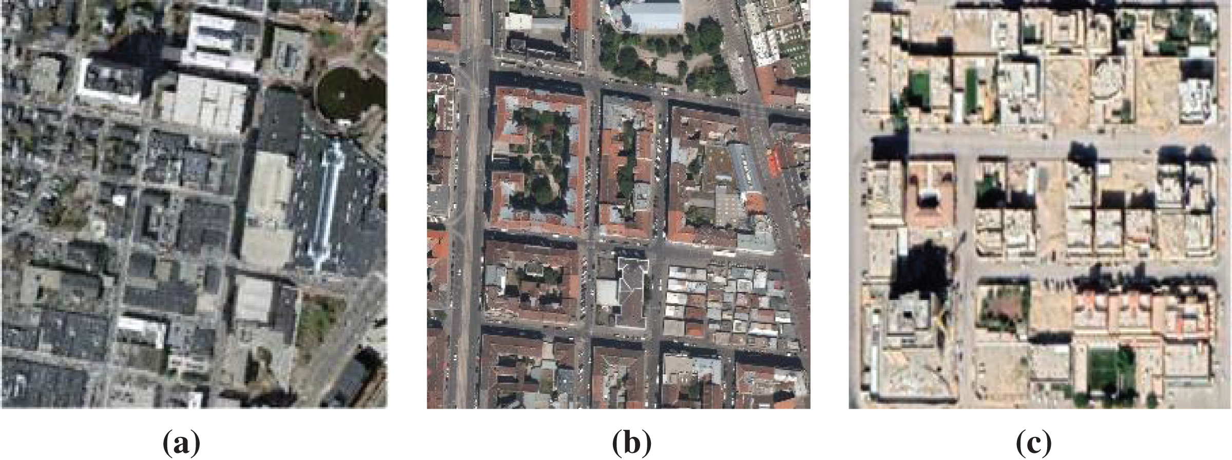
There are a few numbers of datasets that have been presented for the automatic building detection task. These public datasets were called Inria (Maggiori et al., 2017) and Massachusetts datasets (Saito, Yamashita & Aoki, 2016). We have extracted samples from these datasets are shown in Figs. 1A and 1B. Inria dataset covers 810 km aerial satellite-colored images with a spatial resolution of 0.3 m. Each image resolution in Inria dataset is 5,000 × 5,000 pixels. The dataset was collected from several cities. It consists of high densely populated areas and low densely populated areas. The Massachusetts dataset covers 340 km2 aerial satellite-colored images. The dataset was collected from Boston in the United States which covered mostly urban and suburban areas. The dataset contains several buildings sizes and structures. The dataset contains 151 aerial images, with resolution 1,500 × 1,500 pixels.
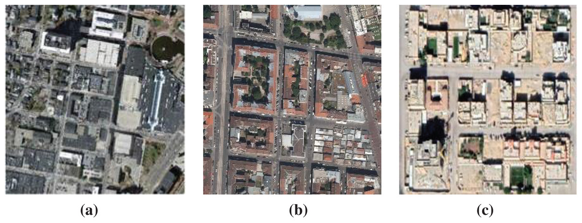
Figure 1: Different building samples from different cities: (A) Boston, (B) San Francisco, (C) Riyadh City.
In the desert environment, there are real challenges that are facing the automatic building detection algorithms. A sample patch from our collected benchmark dataset in Riyadh City is shown in Fig. 1C. Such challenges are low contrast of the image, the absence of colored building roof, shadows effect, and the complex desert background. All these previous challenges are not included in the Massachusetts and Inria datasets. Therefore, there is a real need to collect a new dataset for similar building detection tasks.
Building boundary extraction through the traditional image processing algorithms had been developed through many algorithms (Ghanea, Moallem & Momeni, 2016). These algorithms were based on pre-processing stage followed by the segmentation algorithm such as thresholding, edge detection, Hough transform, and k-means clustering (You et al., 2018), (Bachiller-Burgos, Manso & Bustos, 2017), and (Pushparaj & Hegde, 2017). On the other hand, there are supervised techniques that have utilized features extraction for building detection such as Local Binary Pattern (LBP), Histogram of Oriented Gradients (HOG) (Konstantinidis et al., 2016), Grey Level Co-occurrence Matrix (GLCM) (Zhang et al., 2017), and Scale-Invariant Features Transform (SIFT) (Sirmacek & Unsalan, 2009). Then, a classification procedure is applied to the extracted features to classify pixels such as random forest, AdaBoost, and Support Vector Machine (SVM) (Chen, Li & Li, 2018a). However, these consequences procedures are complex in implementation which consumes a lot of processing time and lacks robustness and generalization ability.
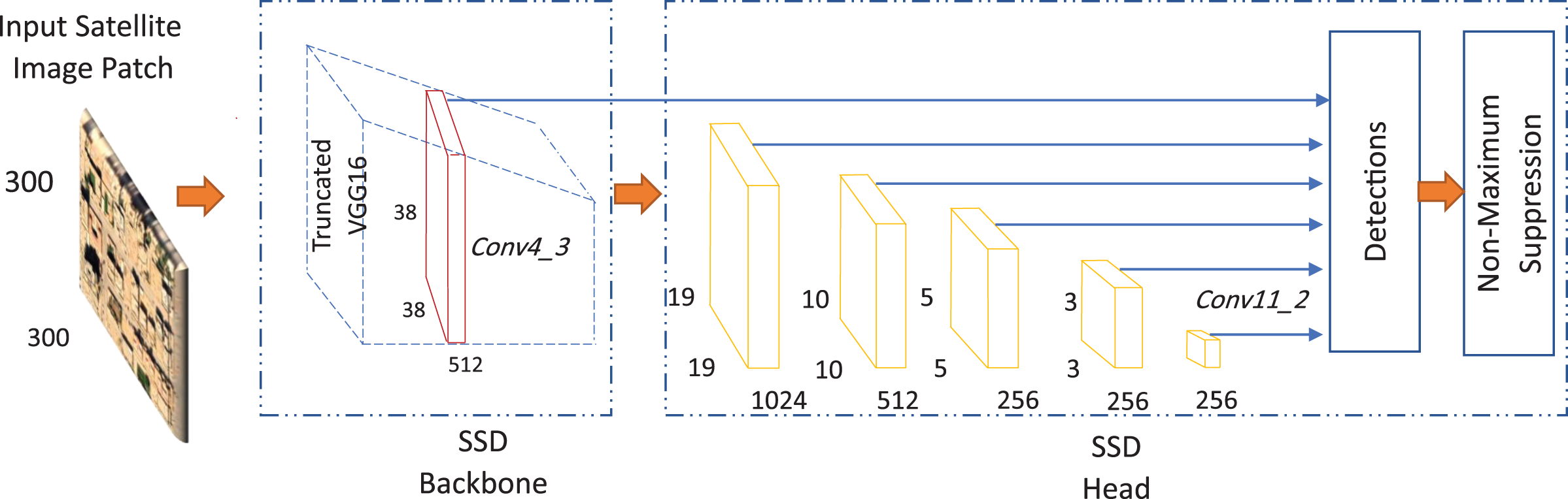
In recent years, in favor of the development in the hardware computational capabilities and the availability of data sources for the training process, deep learning has emerged as a powerful tool for several computer vision tasks. Convolutional Neural Network (CNN) is the first architecture LeNet introduced by LeCun which has the capabilities to automatically extract features through convolutional learnable filters (Lecun et al., 1998). Deep learning architectures mostly employ this powerful capability to extract the target features. In the first version of deep learning detectors, CNN is utilized to suggest proposal regions and consequently localization of the object bounding box. To save time-consuming during to consequences steps, CNN is used to classify objects and at the same time, an additional part of the network can be utilized to localize objects. Liu et al. (2016) has introduced single-shot detector (SSD) which consisted of two main parts: SSD backbone and SSD head as shown in Fig. 2. SSD Backbone has a pre-trained deep neural network that is responsible for the extraction of object features inside the input image. SSD head is responsible for determining of accurate bounding box surrounding the object related to its class and its probability.
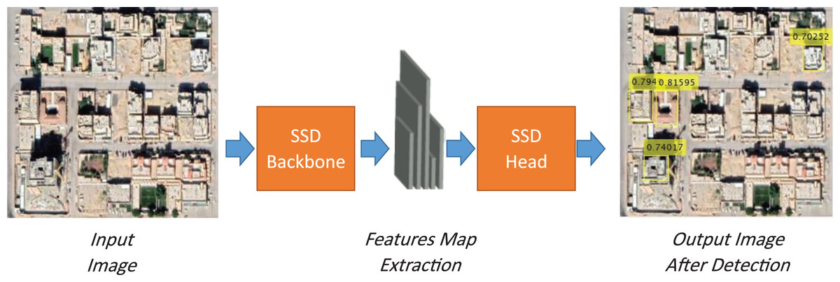
Figure 2: SSD detector pipeline for building detection.
However, the SSD detector performance is very weak in low contrast images as shown in Fig. 2, as there are several missing buildings. Moreover, the detection results suffer from low confidence. Therefore, to increase the performance of CNN capabilities for SSD object detection, there is a need to modify the SSD deep detector backbone or head. The features discrimination power embedded with the SSD backbone can achieve a significant improvement. There are several approaches that can be performed to enhance the performance of the SSD backbone such as deep features fusion (Shahin & Almotairi, 2020), hand-crafted features fusion (Tianyu, Zhenjiang & Jianhu, 2018), and head fusion module (Zhai et al., 2020). Visual attention mechanism helps also the classification network to increase its performance through sharing weights from one network to another network (Guo et al., 2016). On the other hand, the SSD head that is responsible to minimize the intersection over union (IOU) of the detected class object, can be enhanced through the optimization of the network loss function (Zhao et al., 2020) and anchor-boxes dimensions optimization (Mazzia et al., 2020). In this paper, we utilize a deep learning detection approach based on single-stage detector type which is SSD which provides simplicity, accuracy, and speed. Moreover, several modifications are applied to the state-of-the-art SSD detector. We utilize the saliency visual attention mapping to increase the detection performance. Moreover, the SSD head is enhanced by optimizing bounding box search space.
The remainder of our paper is organized as follows. “Related Works” discusses the related works for SSD detection applications with focusing on building detection applications. “Material and Methods” discusses our proposed methods with the utilized material during this study. “Results and Discussion” presents the experimental section with the discussion for our results. Finally, “Conclusions” concludes our work and suggests the future work.
Related works
In this section, we introduce the building detection algorithms in the literature. Then, we will focus on the deep learning applications that have utilized the SSD and the visual saliency attention mechanisms in remote sensing applications. Various studies have been proposed for building detection task based on both traditional and deep learning approaches as shown in Table 1.
| Reference | Approach | Image type | Size of dataset | Detection task | System performance |
|---|---|---|---|---|---|
| Ghandour & Jezzini (2018) | Thresholding, morpholoigcal processing. | Aerial RGB images. | 665 buildings in high resolution satellite images. | Buildings detection in suburban areas. | OQP = 92.25% |
| Aamir et al. (2019) | Line-segment detection. | Satellite RGB and gray-scale images. | 163 buildings in 4 high resolution satellite images | Buildings detection in urban areas. | DA = 89.02% |
| Gavankar & Ghosh (2019) | K-means clustering. | Satellite Multispectral images. | 96 buildings in remote satellite images. | Buildings detection in urban areas. | QA = 91% |
| Li et al. (2019) | SSD detector | Aerial RGB images. | 500 aerial images. | Buildings damage detection. | AP = 77.27% |
| Li et al. (2018) | Hough transform guided RCNN. | Aerial RGB images. | 100,000 buildings in 2,000 aerial images. | Building detection in urban, suburban, and rural areas. | AP = 99% |
| Chen et al. (2018b) | Modified RCNN | Aerial RGB images. | 364 aerial images. | Building detection in rural areas. | AP = 94% |
Note:
Abbreviations; OQP, Overall Quality Percentage; DA, Detection Accuracy; QV, Quality Value; AP, Average Percision.
There are several articles in the literature aimed to construct an automatic building detection system which is based on several segmentation algorithms (Hermosilla et al., 2011). Ghandour & Jezzini (2018) presented an automatic building detection algorithm based on aerial satellite images. Their algorithm was based edge detection and the features extracted from image color invariants. They achieved an overall quality percentage 92.25%. However, their system was applied on a limited size dataset with a lack of generalization ability due to using several morphological processing in their algorithm. Aamir et al. (2019) presented a traditional system to detect buildings in low contrast images. The authors employed the wavelet information combined with singular value decomposition (SVD) to overcome the low contrast image appearance. Then, a perceptual grouping segmentation algorithm was applied to extract the building boundary. Their study achieved a detection accuracy 89.02%. However, their study was applied to only 163 buildings in their dataset. Gavankar & Ghosh (2019) introduced an automated system to extract building footprints from high-resolution multispectral images. In addition, the authors introduced a K-means clustering algorithm to extract building footprint. Nevertheless, their system achieved a correctness value of 0.94 and a quality value of 0.91. However, their system was examined only for 96 buildings. All traditional methods were based on building boundary detection or roof building detection through their color. Some of these methods utilized LiDAR information to be fused with aerial images to increase performance. These algorithms were validated on a small scale of building datasets and also lacked to be widely applied (Sohn & Dowman, 2007).
Another approach to establish an automatic building detection is the deep learning approach. However, there are a few numbers of articles that applied building detection algorithms using deep learning in aerial satellite images. These studies included building damage and collapsed building detection after the earthquake. Li et al. (2019) employed the SSD detector for the building damage detection task. They utilized the SSD with no modification in its main architecture. They applied their detection algorithm to the Hurricane-Sandy dataset and their system achieved in favor of using data-augmentation 77.27% average precision. Li et al. (2018) collected RGB satellite images from Google Earth. They collected 2,000 low resolution images from Google Earth, that covered urban, suburban, and rural areas in China. They noticed that the building detection accuracy was varying according to the area of application. They applied several approaches such as faster RCNN which achieved average precision 75.8%, 70.2%, and 58.5% in urban, suburban, rural areas, respectively. The region-based fully convolutional networks (R-FCNs) achieved average precision 75.8%, 70.2%, and 61.2% in urban, suburban, and rural areas, respectively. They employed the guiding technique with Hough transform features which increased the average precision to 70%. Chen et al. (2018b) introduced a deep learning system to detect oriented buildings in aerial extracted from rural areas. The authors modified the SSD detector to consider the building orientation angle. In addition, their system has achieved average precision reached a value of 94%. However, the experiments were only applied on 364 aerial images for both training and testing processes.
The saliency guiding technique has increased the performance of the deep learning detectors. Hu et al. (2018) introduced an aircraft detection algorithm in the aerial satellite images. They utilized a modified version of faster RCNN. They utilized ROI saliency attention in the latent layer to increase the visual inference capabilities of deep faster RCNN. They achieved a high average precision value reached to 99%. However, they ignored the computational cost analysis of their proposed system. Li et al. (2020) introduced a global-local saliency algorithm for ships detection in the satellite aerial images. They utilized a faster RCNN detection algorithm and combined saliency features mapping besides the deep features to feed another proposed a global attention network to increase the detection accuracy. The average precision reached 72.99%. However, it consumed a lot of processing time. Moreover, they extended their system to the third stage which increased their system complexity. Du et al. (2019) had applied a saliency-guided SSD detector to several objects detection in SAR images. The authors used a fusion mechanism between two streams of VGGNet to increase the system performance. The first stream represents the deep features, and the second stream represents the saliency deep features. The system achieved 91% precision and 96% recall. However, the availability of SAR images represents a challenge more than satellite aerial images. On the other hand, they did not examine a high-performance pre-trained networks such as ResNet architecture, and the fusion between saliency and spatial deep features was extended through all SSD network which increased the learnable parameters and complexity.
From the previous literature, there is no benchmark dataset for the low contrast buildings dataset in the desert environment. There are limited benchmark datasets in the literature that covered building areas. We have found that the SSD detector has not been applied to solve the building detection tasks in the low contrast desert environment. Most of the previous detection algorithms neglected the data-augmentation stage before the detection step. The visual attention mechanism has been proved as an excellent tool to increase the SSD performance. However, it has not been applied to the building detection domain. The visual saliency attention fusion with the SSD network was very complex and applied to other object detection tasks. Therefore, there is a need to be applied in the building detection task.
In this paper our contributions are as follows: (1) we have proposed a novel deep learning architecture for building detection in high-resolution satellite images based on saliency attention mechanism, (2) we have collected a new dataset for buildings in the desert environment with low contrast appearance in Riyadh City, (3) we have proposed a special data augmentation to overcome low contrast desert environment effect upon the images, (4) we have proposed two proposed SSD backbone architectures based on saliency visual attention, (5) we have investigated the fusion function between spatial and saliency features map, (6) we have estimated the optimized the anchor-boxes sizes inside the SSD head to increase the system performance, and (7) the proposed network proved its super-capabilities compared to the state of the art one and the previous methods.
Materials and Methods
Material
To establish our research idea for building detection inside a desert environment, we have collected a dataset for buildings in high-resolution satellite images from Riyadh City, Saudi Arabia. The image size is 3.6 Gigabytes in ECW compression format. We have utilized QGIS Pro to extract the small patches from the large image in JPEG compression format with zoom ratio 100% and scale 1:1,582. The total number of images was 500 images with a resolution 300 × 300. The total number of buildings in our dataset reached 3,878 buildings. The annotated buildings have large variations in size, color, overcrowding, and shape inside the dataset. We have also randomly divided the dataset into 80% for training and 20% for testing.
Methods
The state of the art of SSD-backbone consists of a VGG16 pre-trained model which has proven its capabilities to extract the image features representations (Liu et al., 2016). However, the feed-forward model generates only a fixed size for target detection and consequently its score. At the end of the network, the non-maximum suppression is utilized to generate the final detection results. For achieving the multi-scale box techniques, SSD extracts six additional feature maps for the detection starting from the convolutional layer named Conv4-3 to the convolutional layer named Conv11-2 as shown in Fig. 3. The multi-box strategy helps to decrease the computational complexity and the scale invariance of the features map on a specific scale. The SSD network consists of the original VGG16 plain deep network that produces location sets corresponding to a set of specific-size target. Each class category has its scores for each object that exists in each target frame. By utilizing the non-maximum suppression, the detector generates the final detection results. Moreover, each additional feature layer in the VGG16 pre-trained network uses a set of convolution filters to get a specific detection result. These convolution kernels produce a score for each class from the object’s default frame position.
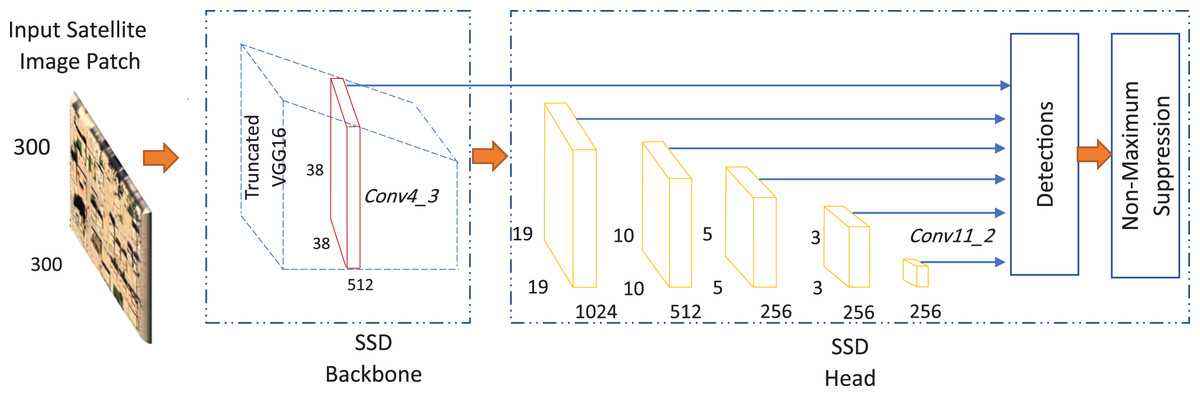
Figure 3: The state-of-the-art of the single shot multi-box detector (SSD).
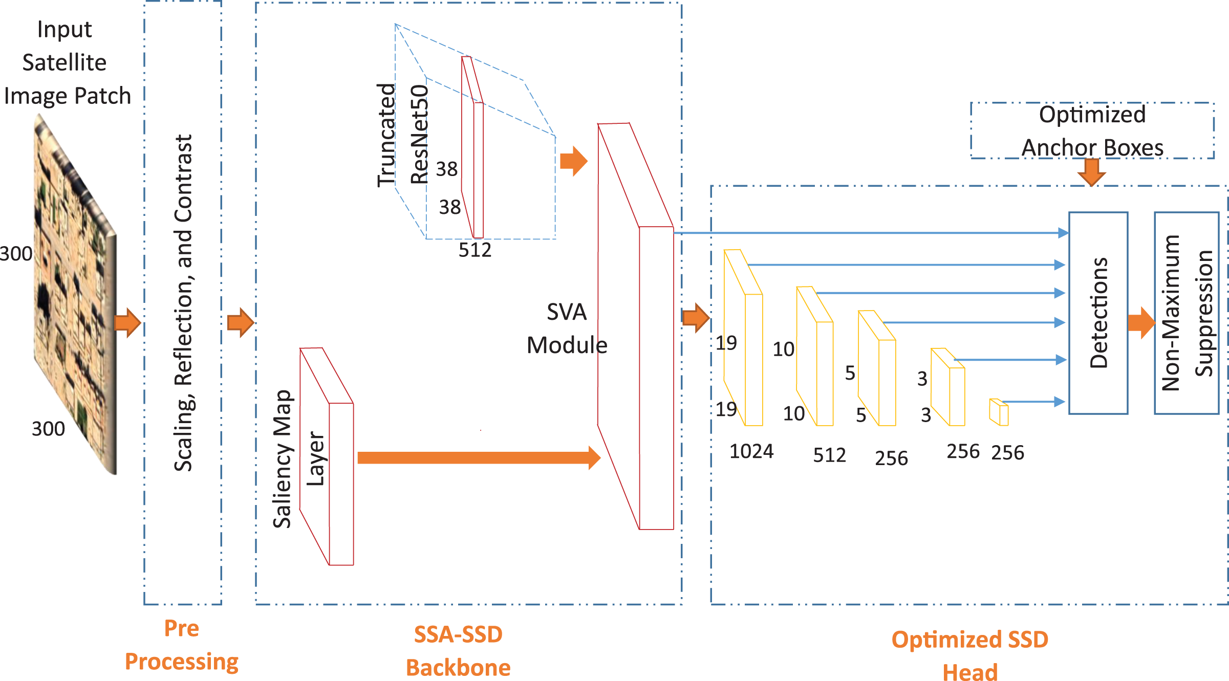
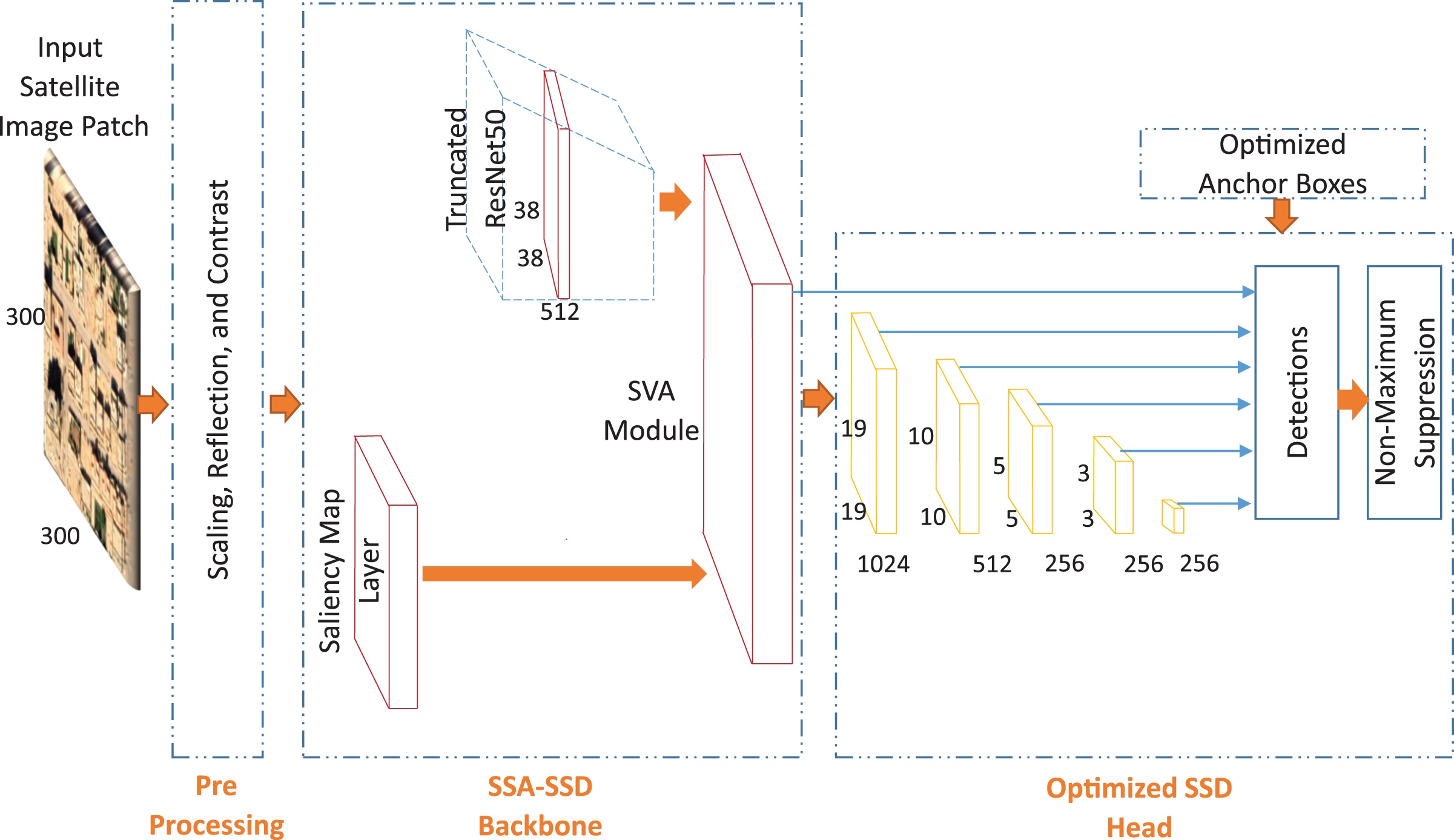
In this paper, we propose a novel saliency attention SSD approach for building detection task in the desert environment. We propose two approaches consists of three main parts which are pre-processing, SSD backbone, and optimized SSD head. We propose light saliency attention with no VGG16 as shown in Fig. 4. Then, we propose a higher depth saliency attention with VGG16 truncated pre-trained network as shown in Fig. 5.
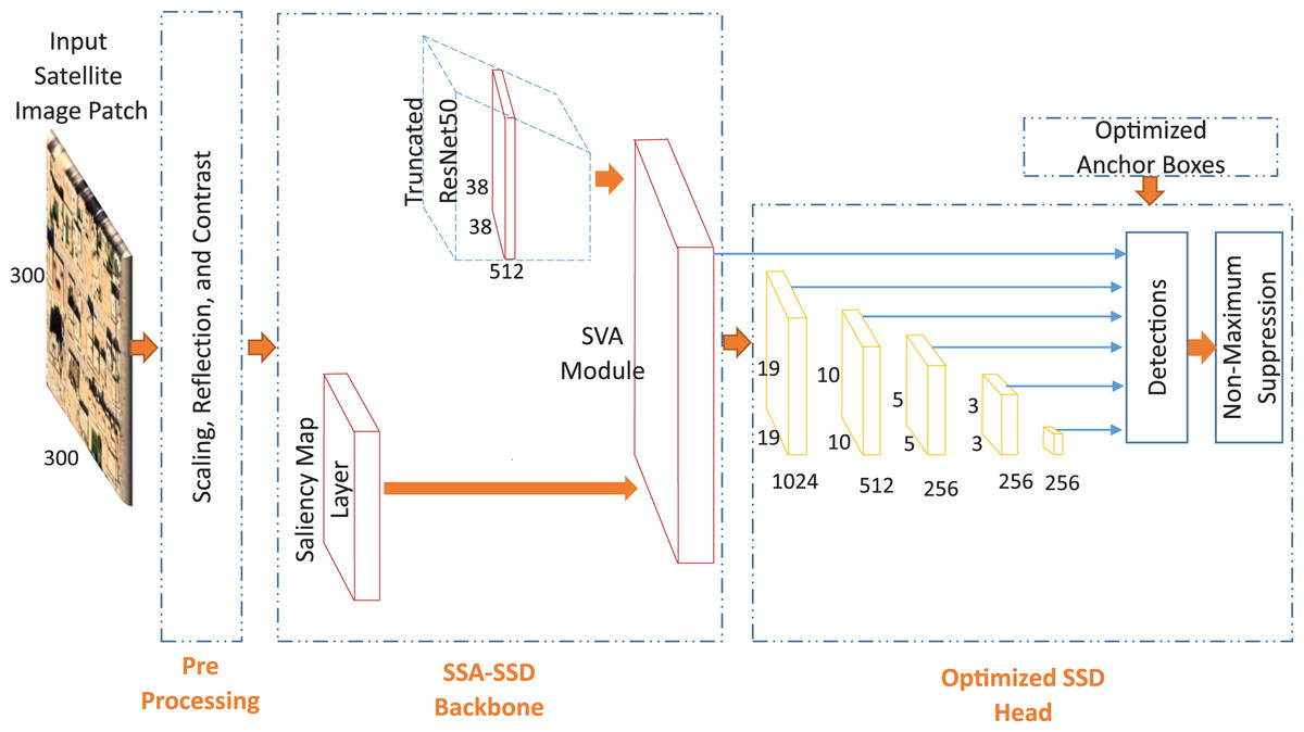
Figure 4: The first proposed approach for buildings detection in low contrast images of the desert environment.
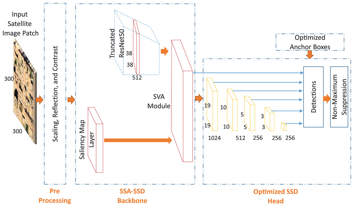
Figure 5: The second proposed approach for buildings detection in low contrast images of the desert environment.
Pre-processing
The pre-processing stage has proven its super capabilities to increase the deep SSD detector (Li et al., 2019). In this paper, we employ the data-augmentation process to expand the size of the input training samples and increase the variations of input training dataset. These variations can help the detector to overcome the low contrast problem of the desert environment and non-colored roof. In this paper, we employ contrast, scaling, and rotations. In contrast technique, we adjust the input RGB image with a pre-defined value of contrast, brightness, hue, saturation, and value from hue-saturation-value (HSV) color space. These variations in contrast and saturation and brightness increase the variations of coloring conditions inside the input images. We also add the scaling augmentation to have different scales of input buildings. The X, Y reflection augmentation techniques are also be added to increase the size of the training images. The parameters for each technique are set to each technique as shown in Table 2.
| Technique | Value | |
|---|---|---|
| 1 | Contrast | 0.2 |
| 2 | (H,S,V) | (0,0.1,0.2) |
| 3 | Brightness | 0.2 |
| 4 | Scaling | (0.5,1.5) |
| 5 | X-Reflection | – |
| 6 | Y-Reflection | – |
SA-SSD backbone
We develop the traditional backbone of SSD which is responsible for the classification of the detected objects based on two methods. The first method is based on the saliency features map and the second method is based on the attention unit from the saliency features map to spatial features map of VGG16 architecture. To achieve the best performance, we develop a saliency visual attention (SVA) module and a latent fusion module.
Truncated pre-trained network
The detection accuracy of where the buildings are located in the images is mainly depending on the extracted deep features. Each pre-trained network has its own features discrimination capability. Therefore, in this paper, we employ several truncated pre-trained networks after removing the final classification layers. These networks are VGG16, ResNet50, and Resnet101. We specify the feature extraction layer in each network as follows: layer named CONV 4_3 for VGG16 network, layer named activation_40_relu for ResNet50 network, and layer named res3b3_relu for ResNet101 network. In this paper, we apply these networks directly to the state-of-the-art SSD detector. Then, We investigate the effect of our proposed saliency layer to the state-of the-art SSD detector. Moreover, We investigate two different approaches to extract the saliency features. The first approach as shown in Fig. 4, is based on applying the output saliency features map to the VGG16 truncated network. The second approach as shown in Fig. 5, is based on applying the output saliency features map to the fusion function directly. This investigation helps to study the features discrimination power between our two proposed approaches.
Enhanced spectral saliency residual
Generally, the desert satellite remote sensing image has low contrast. Therefore, we aim to employ spectral saliency features to enhance the buildings’ detection task. The big challenge in such images is the appearance of uneven lands, which may confuse the detector during building detection. The saliency features map helps the detector to neglect the false-negative regions such as uneven lands and boost the true-positive regions where the buildings are genuinely located in the image. Therefore, enhancing true-positive regions compared to false-negative ones will increase the average precision (AP), recall, and F1-Score performance, reflecting the detection performance. Moreover, This increases the intersection over union ratio (IOU) between the detection target and the ground truth.
The saliency features developed by Itti’s concerned with the difference of center-surrounded to extract the saliency features based on log-log scale (Hou & Zhang, 2007). Although Itti’s method has simple calculations, it lacks robustness. The spectral saliency residual is used to overcome Itti’s method drawbacks. However, there is still a need to develop a method that can extract features map in poor contrast image as in our detection task. On the other hand, the saliency features have been embedded with the SSD detector and have increased its performance (Du et al., 2019). In our proposed approach, we develop an Enhanced Spectral Saliency Residual (ESSR) layer as shown in Algorithm 1. It consists of two main stages: the first stage is the extraction of saliency features map; the second stage is enhancement of the saliency features map. Moreover, we establish the saliency features fusion on the SSD backbone with no need for several multi-scale fusion function repetition through all SSD network.
| Read the satellite input image I. |
| Extract the spectral information using fast fourier transform (FFT), SI = FFT2 (I) |
| Extract the phase spectrum from spectral information, PS = angle (SI). |
| Compute the log amplitude spectrum from the spectral information as in Eq. (1). |
| Compute the average spectrum as in Eq. (2). |
| Subtract the log spectrum from average spectrum to get the spectral residual as in Eq. (4). |
| Compute the saliency map image as in Eq. (5). |
| Apply a contrast adjustment to the residual saliency features. |
| Apply histogram equalization to the adjusted saliency features map. |
| Obtain the enhanced spectral saliency residual (ESSR) features map. |
The log-log representation of input images introduced by (Itti, Koch & Niebur, 1998). It suffers from scale invariance and the sampling is not well-distributed. The log spectrum representation L(f) introduced to overcome the log-log representation drawbacks of the input image and it can be defined as (Hou & Zhang, 2007):
(1)
To extract the saliency features map, the average spectrum A(f) can be defined as the convolution process of the input spectrum representation L(f) can be defined as:
(2)
where h(f) is an n
 n matrix which is defined as:
(3)
The spectral residual R(f) represents the statistical singularities related to the input image. The log spectra share the similar trends for the same objects and it can be defined as:
(4) where α is set to be the control parameter in the range (1, 1.5).
We extract the saliency map that represents the inverse Fourier transform of the log-spectra output as in Eq. (5) (Hou & Zhang, 2007).
(5)
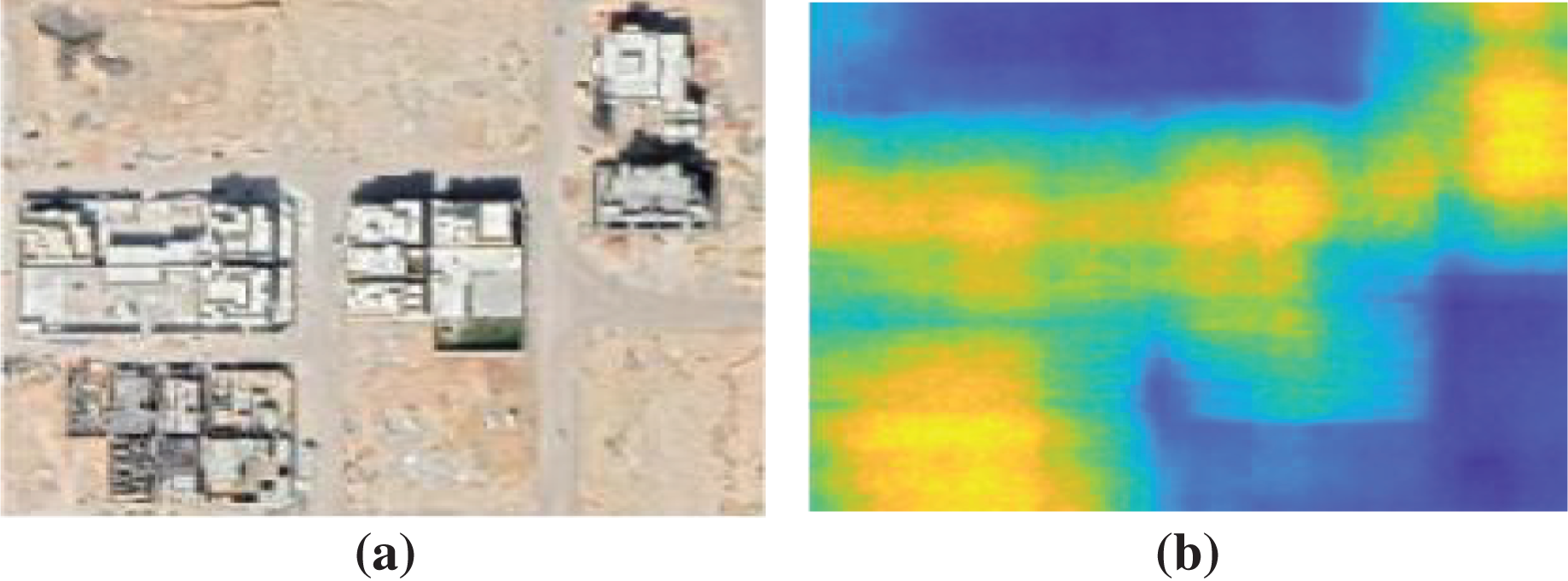
As the low contrast of building images in the desert environment as shown in Fig. 6A, we need to enhance the saliency features map. To perform this enhancement, we apply a contrast adjustment process followed by histogram equalization. These two consequences operations enhanced the saliency features map appearance. As shown in Fig. 6B, the buildings’ areas are differentiated obviously in the saliency spectral color map.
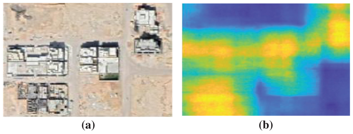
Figure 6: Our proposed ESSR enhancement effect: (A) a sample from original low contrast image; (B) saliency features map.
SVA module
The attention mechanism in the deep networks has been widely utilized to improve several deep architectures (Yi, Wu & Metaxas, 2019). The visual attention mechanism is based on sharing weights from a network to the same network or another network. Yi, Wu & Metaxas (2019) proposed a self-attention mechanism that is based on sharing the attention between the features map and the prediction module. However, in visual detection tasks, there is a need to boost the network vision capabilities with another discriminated features map. In this paper, we propose a new SVA unit. In our model, the attention is happening from the saliency features map to the spatial features map. To boost our SSD backbone classification capabilities, we perform an attention process between saliency and spatial deep features in addition to the early visual attention mechanism. Du et al. (2019) utilized the fusion in the SSD head by the fusion module to predict targets with multiple features map representation. However, the cost of fusion of the saliency features maps with spatial features along the SSD detector depth increased the training parameters. This reflects on the training and detection cost time. In this paper, we utilize single latent attention between the spatial features map and the saliency features map after enhancement.
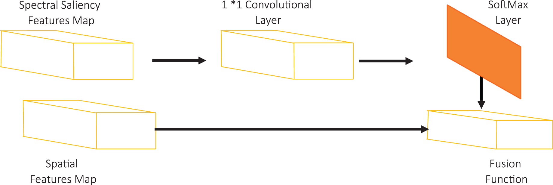
As followed in (Du et al., 2019), we introduce our fusion module structure as shown in Fig. 7. We use a 1 × 1 convolutional layer to adjust the saliency features map dimension with spatial features map to enable the fusion process. Then, we utilize the SoftMax layer to normalize the saliency map. The value Si of a spatial position I in the saliency map represents the saliency score. We assume that the target will achieve the highest saliency score. The SoftMax operation can be defined by:
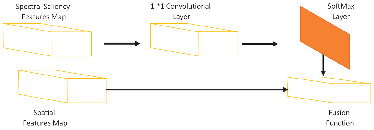
Figure 7: SVA module structure.
(6) where NSi represents the saliency score after normalization inside a spatial position i where i 1, 2, 3, …, n, and n represents the size of saliency features map.
Finally, we apply the fusion function between the saliency features map and the spatial features map which improves the visual representation of the detected objects. In this paper, we investigate three widely used fusion functions that have been utilized in the literature which are addition, multiplication, and concatenation functions.
Optimized-SSD Head
The accurate estimation of the anchor-boxes sizes increases the detection network performance, makes it faster, leads to higher confidence scores (Redmon & Farhadi, 2017). In the previous studies, each dataset was pre-defined with its optimized anchor-boxes (Maggiori et al., 2017; Saito, Yamashita & Aoki, 2016). For our buildings dataset, there is a variation in the size of buildings and there is a need to optimize the anchor-boxes sizes. To optimize the anchor-boxes sizes for the buildings detection task, we follow the same method in (Mazzia et al., 2020). We compute the optimized anchor-box sizes as the following equations:
(7)
(8)
(9)
(10)
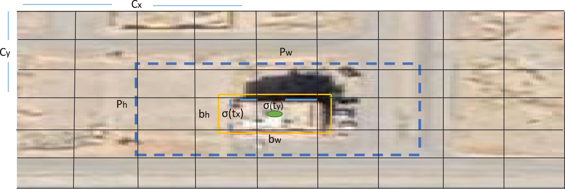
As shown in Fig. 8, x and y are defined as center coordinates for a given image. The SSD head predicts the following coordinates for each bounding box tx, ty, tw, and th, which aims to refine one of its anchors that existed in that selected region inside the image to execute the detection task. After refining process, the SSD head determines each bounding box dimension through four parameters bx, by, bw, and bx. If the cell is offset from the top-left corner of the image by (cx, cy) and the bounding box prior has width and height (pw, ph). For each location, the network generates the bounding boxes with their corresponding confidence σ(to) and C class probabilities pc. Then, Non-maximum Suppression (NMS) with confidence scores are utilized to exclude repetitive detection results and produce the optimized bounding box.
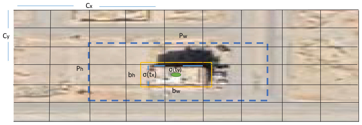
Figure 8: The anchor box used to estimate the buildings location in satellite image.
Results and discussion
During the experiments, we have utilized quantitative metrics which are widely used for similar detection tasks. These metrics are average precision (AP), recall, F1-Score, and intersection over union ratio (IOU). IOU is the ratio as the area of intersection between interpreted box Ibox and ground truth box Gbox, divided by the area of the union of Ibox and Gbox. AP is a widely used metric which can evaluate the detection model by setting several recall threshold values (R) (0, 0.1, 0.2, . . . , 1). The following equations define these metrics:
(11)
(12)
(13)
(14) where TP represents the true positive values, FN represents false negative values, Rn represents the set of recall values, and the APr value represents the maximum precision related to each recall threshold. Besides that, we visualize several examples of our detection results and compare our proposed approach with the others in the literature. Moreover, we perform computational cost analysis for our proposed method vs the previous methods.
Our experiments are performed using MATLAB 2020b. The system hardware specification is containing Quad-Core 2.9 GHz Intel i5 with internal memory RAM 16 GB. The training process is done through GPU NVIDIA Quadro 5,000 with internal memory 16 GB RAM and computing capability 6.1. We set the training parameters as follows: Adam optimizer, 250 epochs, and 0.0001 initial learning rate value.
Experiment1
In this experiment, we investigate the effect of the data-augmentation stage with the state-of-the-art method SSD detector for our building detection task. As shown in Table 3, SSD detector has worked better after data-augmentation procedure and it has achieved 60% average precision, 84% recall, 80.80% F1-Score, and 67.68% IOU.
| AP (%) | Recall (%) | F1-score (%) | IOU (%) | |
|---|---|---|---|---|
| Without augmentation | 56.0% | 78.2% | 76.5% | 62.6% |
| With augmentation | 60.00% | 84.00% | 80.80% | 67.68% |
From experiment 1, we have noticed that the data augmentation increase the SSD detector performance and Table 3 obviously visualized that all indices have been increased. The AP has been increased by 4%, the recall has increased by 5.8%, F1-score has been increased by 4.3%, and IOU has been increased by 5%. At the first moment, the researchers may think that the data-augmentation detection results on the same target dataset should be similar to the original dataset. However, in deep learning algorithms especially the detection algorithms; the data-augmentation techniques improve the detection results. Moreover, the data-augmentation with the SSD detector did not cause over-fitting while the training process. From these results, we have concluded that our proposed data-augmentation parameters can increase the performance of the SSD detector and can be generalized for the other detectors.
Experiment2
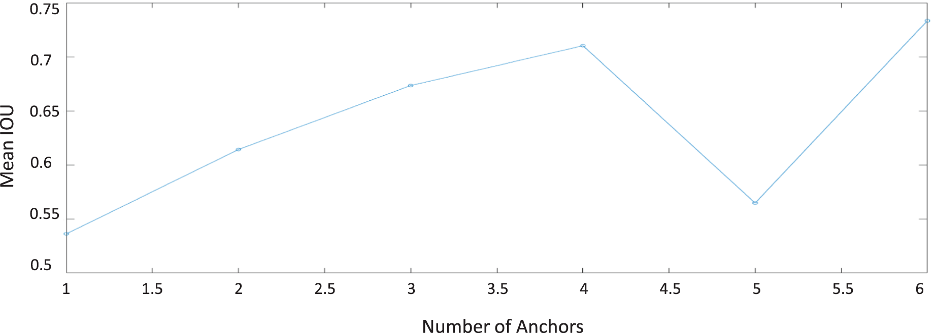
In this experiment, we apply the anchor-boxes size estimation algorithm to our dataset (Redmon & Farhadi, 2017). Generally, it was proven that this stage makes the detection task faster (Mazzia et al., 2020; Redmon & Farhadi, 2017). After running the estimation algorithm, the best anchor-box sizes have been achieved at six anchor-boxes as shown in Fig. 9. The estimated mean IOU at size anchor-boxes has reached to 73%.
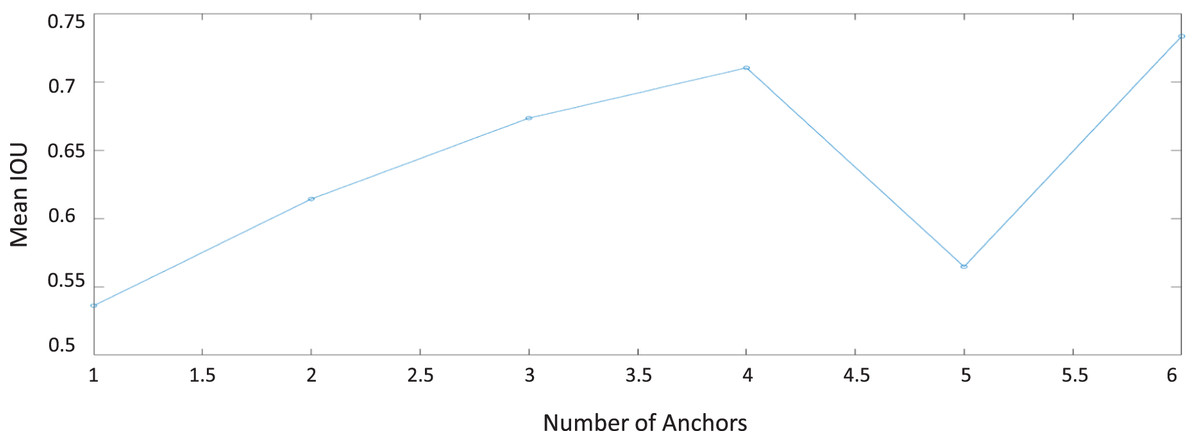
Figure 9: Optimal anchor-boxes size estimation for our building dataset.
From this experiment, we have noticed that the six estimated anchor-box sizes are varying in height and width, as shown in Table 4. This variation can be explicated as our collected buildings dataset contains many buildings with different size characteristics. Therefore, as shown in Fig. 9, increasing the number of anchors cannot ensure the improvement of the mean IoU measure and the detection accuracy. To overcome this problem, dividing the buildings dataset into sub-classes according to their size is essential to increase the mean IOU percentage. In the next experiments, we have generalized both data-augmentation and optimized anchor-boxes to all algorithms to achieve the best performance.
| Width | Height | |
|---|---|---|
| Anchor box 1 | 27 | 26 |
| Anchor box 2 | 30 | 61 |
| Anchor box 3 | 46 | 43 |
| Anchor box 4 | 67 | 33 |
| Anchor box 5 | 47 | 73 |
| Anchor box 6 | 75 | 62 |
Experiment3
In this experiment, we propose a comparison between the state-of-the-art methods to investigate the performance of each detection algorithm and the utilized pre-trained network. In this experiment, we compare VGG16, ResNet50, and ResNet101 as pre-trained networks. Additionally, we compare Fast RCNN, Faster RCNN, and SSD architectures as a detection algorithm.
From this experiment, we have noticed that the SSD detector with ResNet50 base network has achieved the best performance for F1-Score 80.8%, and IOU 69.72%. However, the SSD detector with ResNet101 base network has achieved the best recall value 88.9%. The SSD with VGG16 base network has achieved the best AP value of 60%. On the other hand, the fast RCNN detector with a VGG16 base network has achieved the worst performance through all detectors. It has achieved 40.67% AP, 69.37% recall, 66.89% F1-Score, and 48.34% IOU.
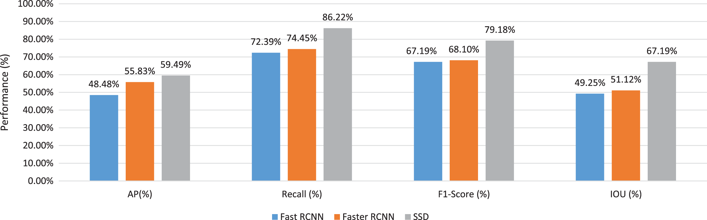
To investigate the best detector architecture and the best base network for our detection task, we take the average values for fast RCNN, faster RCNN, and SSD detectors as shown in Fig. 10. We have concluded that the SSD detector has achieved the best performance for all indices in Table 5. On the other hand, the fast RCNN detector has achieved the lowest performance. It has achieved 44.48% average AP value, 72.99% average recall value, 67.19% average F1-Score value, and 49.25% average IOU value.
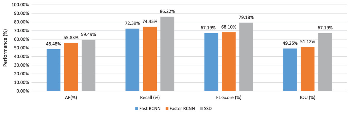
Figure 10: The average values of several evaluation criteria of different pre-trained networks through different detector architectures.
| AP (%) | Recall (%) | F1-score (%) | IOU (%) | |
|---|---|---|---|---|
| Fast Rcnn_VGG16 | 40.67% | 69.37% | 66.89% | 48.34% |
| Fast Rcnn_ResNet50 | 51.12% | 75.15% | 67.22% | 48.47% |
| Fast Rcnn_ResnNet101 | 53.66% | 72.65% | 67.46% | 50.93% |
| Faster Rcnn_VGG16 | 56.80% | 75.56% | 69.63% | 53.95% |
| Faster Rcnn_ResNet50 | 57.01% | 75.11% | 66.86% | 50.88% |
| Faster Rcnn_ResnNet101 | 53.69% | 75.63% | 65.61% | 48.89% |
| SSD_VGG16 | 60.00% | 84.00% | 80.80% | 67.68% |
| SSD_ResNet50 | 59.31% | 85.71% | 80.84% | 69.72% |
| SSD_ResNet101 | 59.15% | 88.95% | 75.91% | 64.18% |
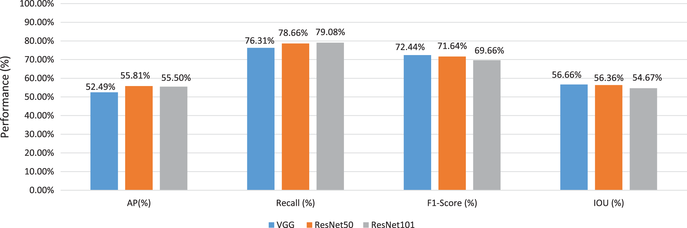
On the other hand, to investigate the best base architecture, we take the average values for VGG16, ResNet50, and ResNet101 detectors as shown in Fig. 11. We have noticed that the ResNet50 base architecture has achieved the best average IOU value 56.66%. The VGG16 pre-trained architecture has achieved the best F1-Score value 72.44%. We have concluded that the base network that has been utilized in the detector backbone has a significant effect on the performance of the detector. We have concluded that both VGG16 and ResNet50 base network architectures have significant discriminated features for our building detection target.
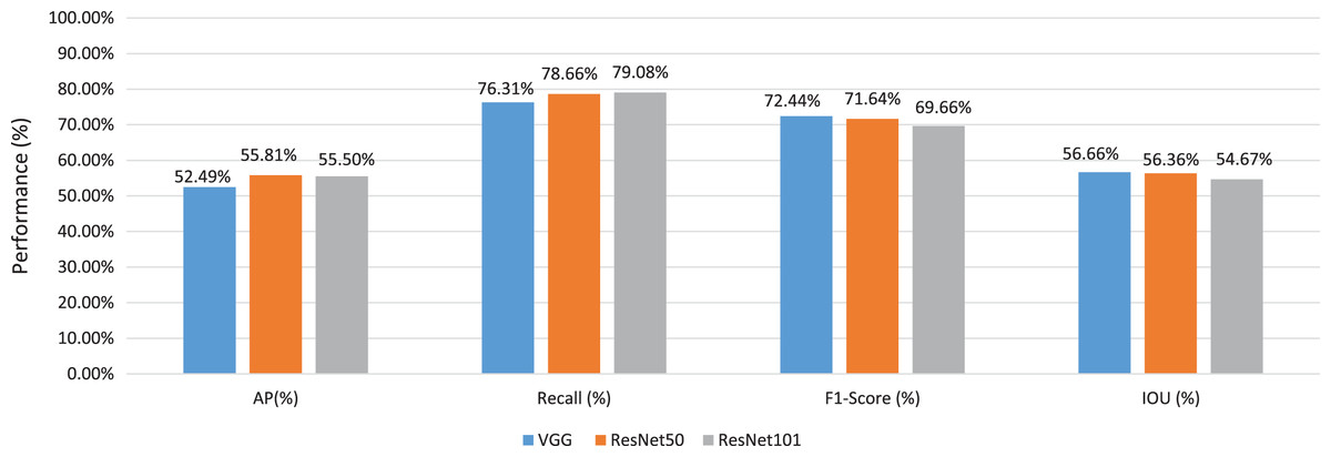
Figure 11: The average values of several evaluation criteria of different detector architectures x through different detector architectures.
Experiment4
In this experiment, we investigate the performance of our SSA-SSD detection algorithm. First, we investigate the performance of our two proposed approaches that have been introduced in Figs. 4 and 5 in the material and methods section. We have employed the add fusion function for the two proposed saliency attention approaches. We have noticed that the second approach has achieved higher performance than the first approach for all evaluation indices as shown in Table 6. The Second Approach has achieved 64% AP, 87% recall, 80.6% F1-Score, and 69.63% IOU.
| AP (%) | Recall (%) | F1-Score (%) | IOU (%) | |
|---|---|---|---|---|
| SVA-SSD ResNet50 approach1 | 62.07% | 84.28% | 62.07% | 69.00% |
| SVA-SSD ResNet50 approach2 | 64.0% | 87.0% | 80.6% | 69.63% |
Second, we have investigated several fusion functions in the SVA module for our second proposed approach as shown in Table 7. The addition fusion function has achieved the best performance for all indices. It has achieved 64% AP, 87% recall, 80.6% F1-Score, and 69.63% IOU. On the other hand, the multiplication fusion function has achieved the lowest performance for all indices. It has achieved 41% AP, 69.3% recall, 61.75% F1-Score, and 57% IOU.
| AP (%) | Recall (%) | F1-Score (%) | IOU (%) | |
|---|---|---|---|---|
| Multiplication | 41.00% | 69.30% | 61.75% | 57.00% |
| Concatenation | 61.42% | 84.83% | 77.50% | 67.36% |
| Addition | 64.0% | 87.0% | 80.6% | 69.63% |
To investigate each component of our two proposed approaches based on the saliency visual attention mechanism, we perform our experiments at two levels. Therefore, we can better decide the impact of each component on the system performance. From the first experiment, it can be observed that the saliency features map is working better with the truncated VGG16. This is important to increase the features discrimination power of the saliency map. We have proven that the high-level features extraction using deep networks is better than direct embedding of the saliency features to the classification network (Arazo Sánchez, 2017). Results show that the introduction of saliency information increase the recall value 1.3% and increase the AP value 4%, which can increase at most the detected buildings accuracy. On the other hand, the introduction of saliency information variate with the fusion function module in the two stream saliency-spatial features maps. In terms of AP, the proposed addition fusion module is about 2.5% higher than the concatenation module. However, In terms of AP, the multiplication fusion module is about 20% lower than both concatenation and addition modules. On the contrary, the saliency guided method in other architecture with another detection target has achieved its best performance with multiplication fusion (Du et al., 2019). Therefore, we have concluded that it is important to investigate the fusion function between spatial and saliency features map according to the network architecture and the detection task.
Experiment5
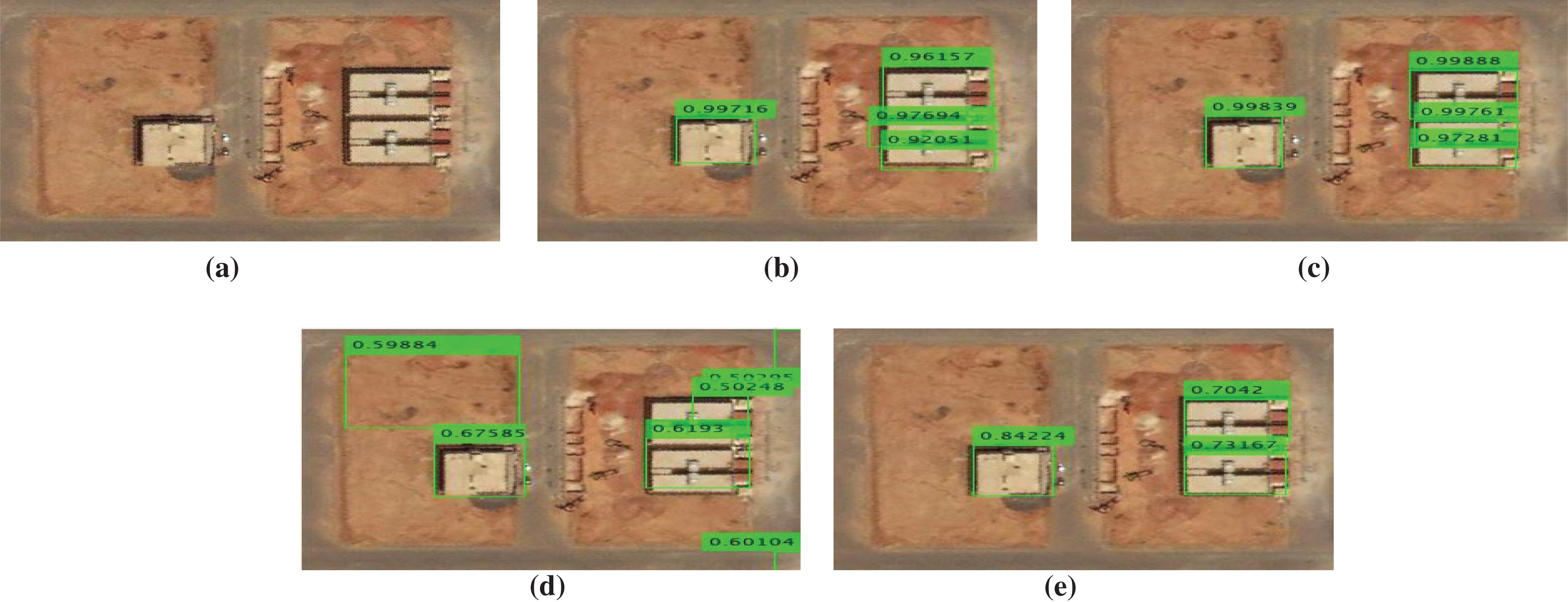
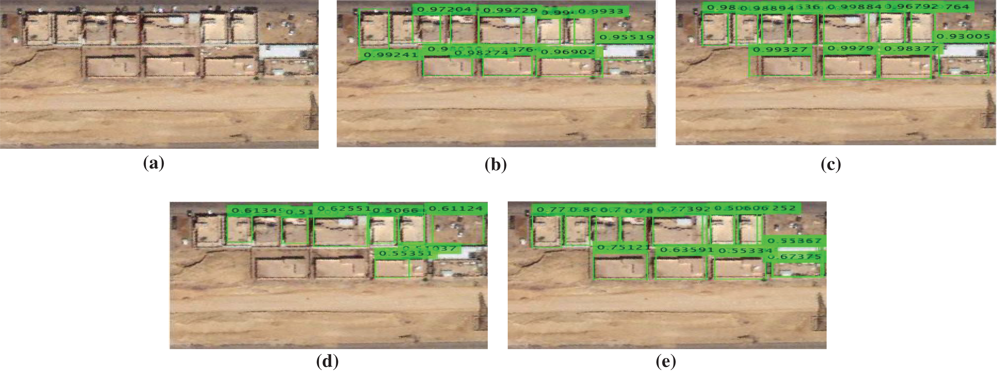
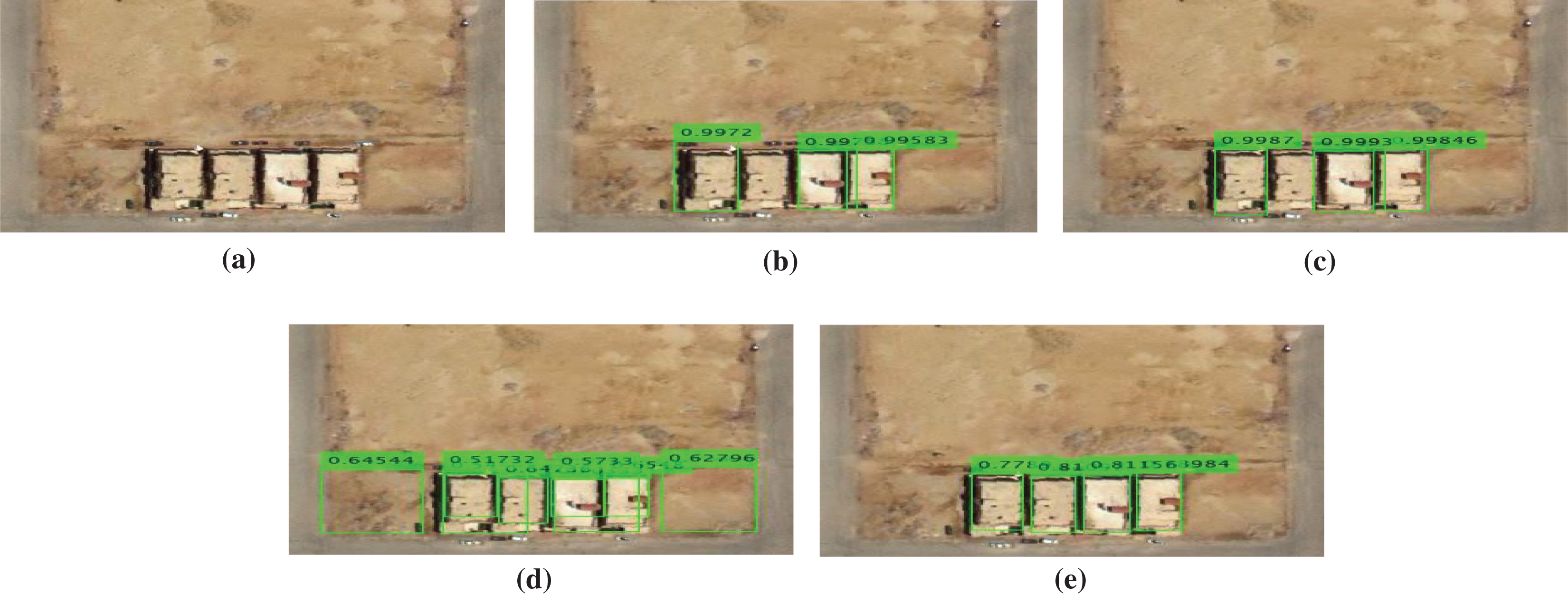
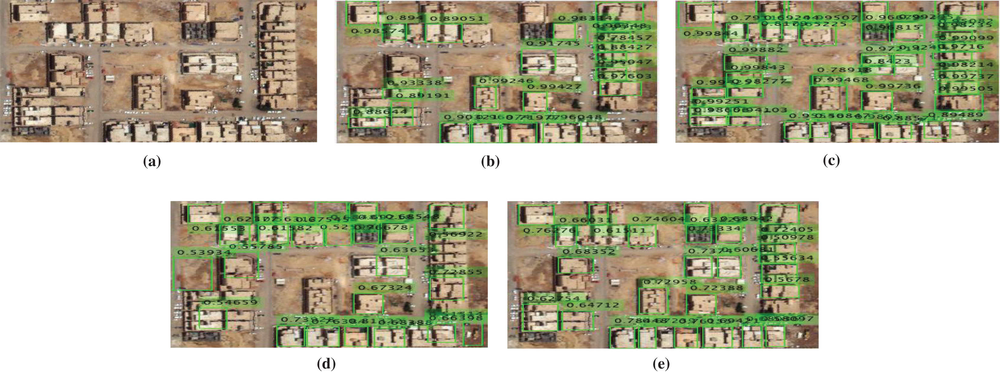
In this experiment, several examples from our building dataset are shown in Figs. 12–16. where green rectangles represent the detected building with the evidence of achieved confidence interval value for each building. The examples consist of high densely populated areas and low densely populated areas.
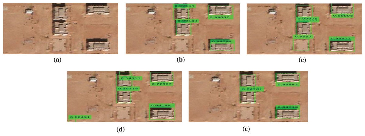
Figure 12: Buildings detection results comparing with the state of the art methods for a test sample image: (A) original image, (B) fast RCNN method, (C) faster R-CNN method, (D) SSD method, and (E) our proposed method (SVA-SSD).
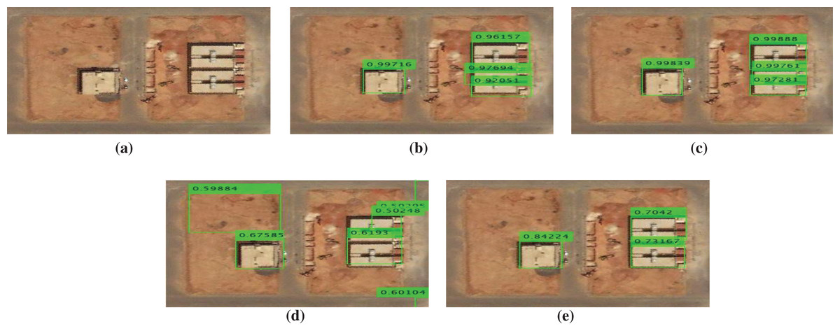
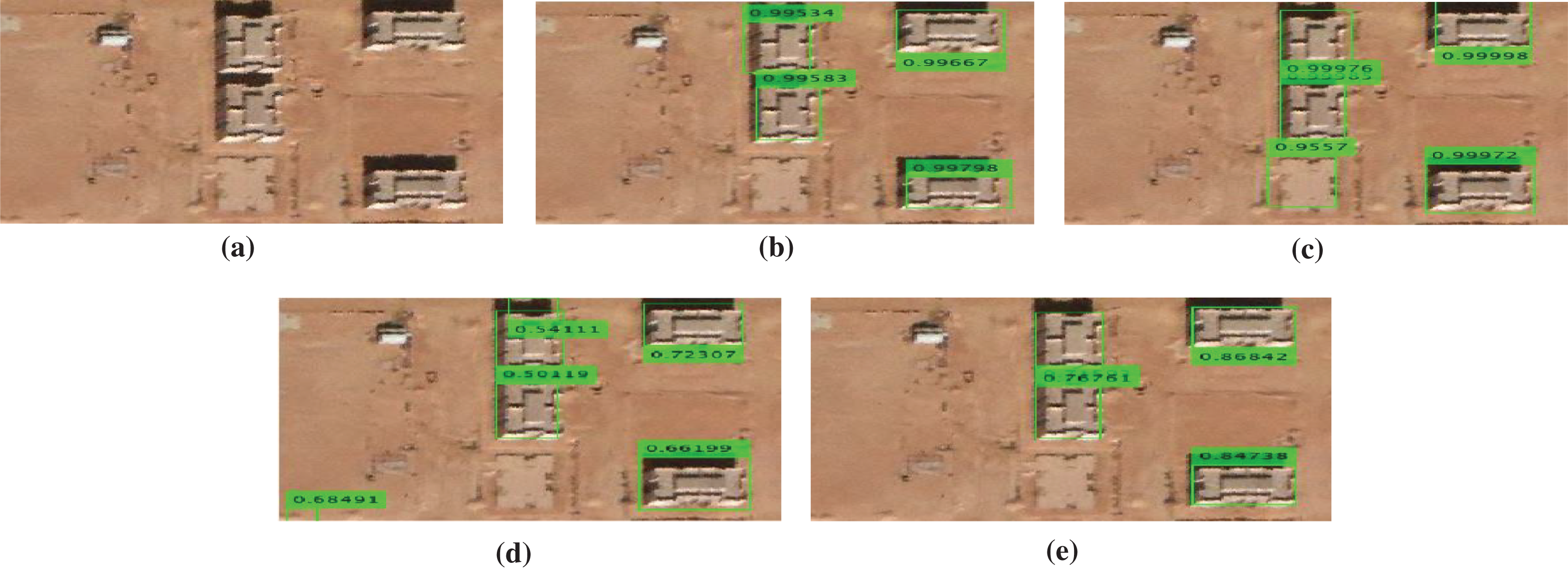
Figure 13: Buildings detection results comparing with the state of the art methods for a test sample image: (A) original image, (B) fast RCNN method, (C) faster R-CNN method, (D) SSD method, and (E) our proposed method (SVA-SSD).
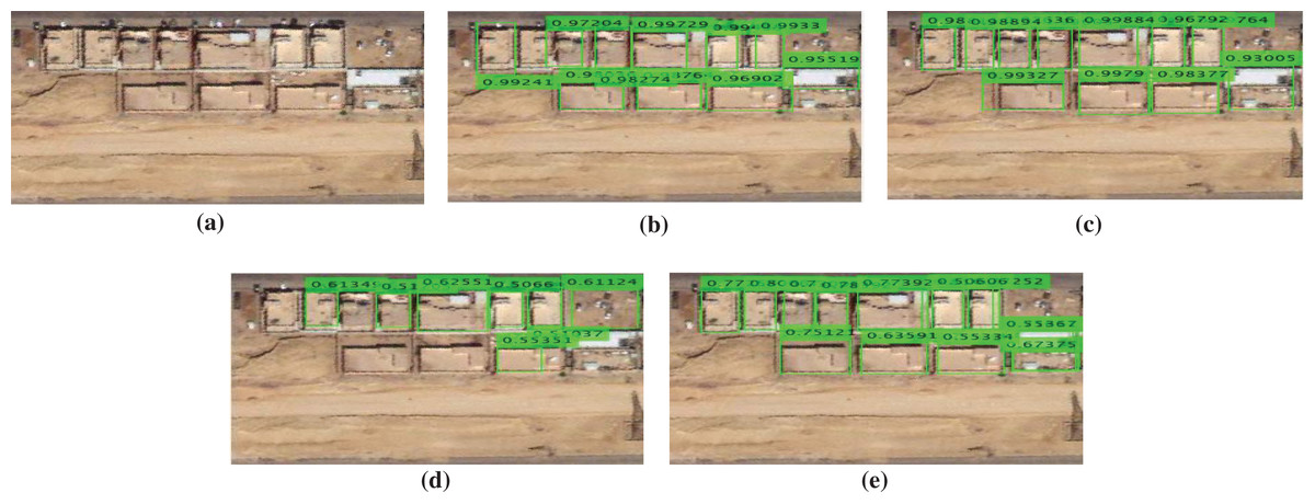
Figure 14: Buildings detection results comparing with the state of the art methods for a test sample image: (A) original image, (B) fast RCNN method, (C) faster R-CNN method, (D) SSD method, and (E) our proposed method (SVA-SSD).
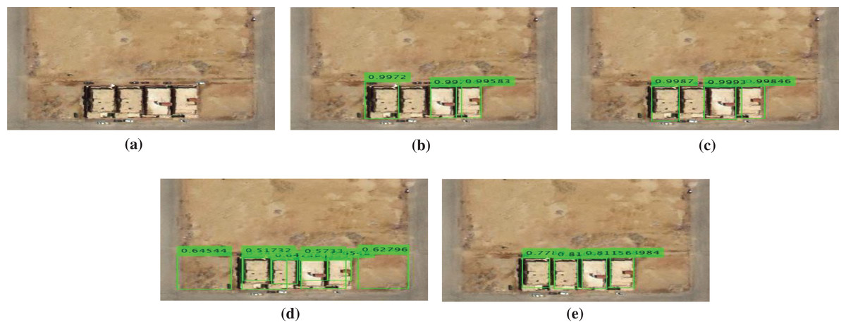
Figure 15: Buildings detection results comparing with the state of the art methods for a test sample image: (A) original Image, (B) fast RCNN method, (C) faster R-CNN method, (D) SSD method, and (E) our proposed method (SVA-SSD).
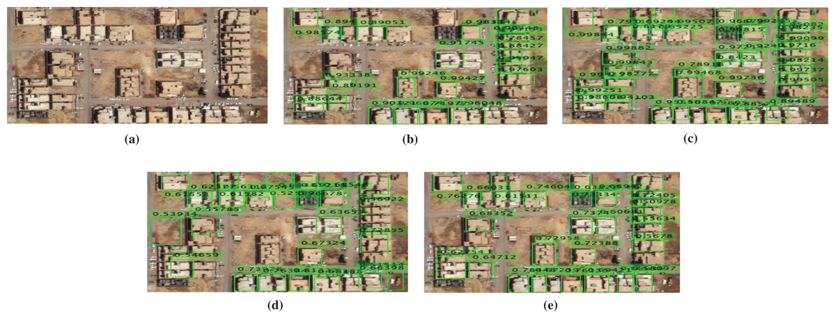
Figure 16: Buildings detection results comparing with the state of the art methods for a test sample image: (A) original image, (B) fast RCNN method, (C) faster R-CNN method, (D) SSD method, and (E) our proposed method (SVA-SSD).
As shown in Fig. 12, our proposed SVA-SSD has achieved the best detection results. On the other hand, the fast RCNN has achieved similar detection results with higher confidence interval values. However, the faster RCNN has achieved bad detection results. The SSD detector has achieved the worst performance with the lowest confidence interval values. In the second example, as shown in Fig. 13, our proposed SVA-SSD has achieved the best detection results. On the other hand, the fast RCNN, and the faster RCNN have achieved similar detection results with high confidence interval values. However, the SSD detector has achieved the worst performance with the lowest confidence interval values. In the third example, as shown in Fig. 14, our proposed SVA-SSD has achieved the best detection results. On the other hand, the faster RCNN has achieved better detection results than the fast RCNN with high similar confidence interval values. However, the SSD detector has achieved the worst performance with the lowest confidence interval values with several missed detection of the buildings. In the fourth example, as shown in Fig. 15, our proposed SVA-SSD has achieved the best detection results. On the other hand, both fast RCNN and faster RCNN has achieved similar detection results with high similar confidence interval values. However, the SSD detector has achieved the worst performance with the lowest confidence interval values with several missed detection of the buildings. In the fifth example, as shown in Fig. 16, we investigate the performance of the detectors in the case of high dense buildings. Our proposed SVA-SSD has achieved the best detection results. On the other hand, the faster RCNN has achieved better detection results than the fast RCNN with high similar confidence interval values. However, the SSD detector has achieved the worst performance with the lowest confidence interval values with several missed detection of the buildings. From this experiment, we have concluded that the saliency visual attention model has increased all buildings’ detection accuracy. Moreover, results indicates that the confidence level of the state-of-the art SDD detector is lower than our proposed detection method. Our proposed method is more stable than both fast and faster RCNN in the detection of high dense building areas. On the other hand, our proposed method is more accurate in the detection of small buildings closer together as shown in Figs. 13–16. We noticed that there is a real need to evaluate the detection results based on both quantitative and qualitative results.
Experiment6
In this experiment, we investigate the computational cost analysis of our proposed method compared to the previous methods as shown in Table 8. We compare between our proposed architecture and different detectors with the same base network ResNet50. We have noticed that faster RCNN architecture has the highest learnable parameters 33.2 M with the longest training time 5,750 min. Although the faster RCNN parameters are very near to fast RCNN, it has a lower training time than fast RCNN. The inference time for both fast and faster RCNN are slightly different. On the other hand, the SSD ResNet50 architecture has the lowest value of 12 M learnable parameters with the lowest training time of 175 min. On the other hand, our proposed method has achieved intermediate 16 M parameters with low training time relative to RCNN architectures. However, It has achieved a near inference time value compared to the SSD-ResNet50.
| Learnable parameters (Million) | Training time (Min) | Inference time (S) | |
|---|---|---|---|
| Fast Rcnn_ResNet50 | 33.2 | 5750 | 0.681 ± 0.089 |
| Faster Rcnn_ResNet50 | 33 | 5500 | 0.684 ± 0.092 |
| SSD_ResNet50 | 12 | 175 | 0.0276 ± 0.006 |
| Our proposed method | 16 | 392 | 0.0329 ± 0.007 |
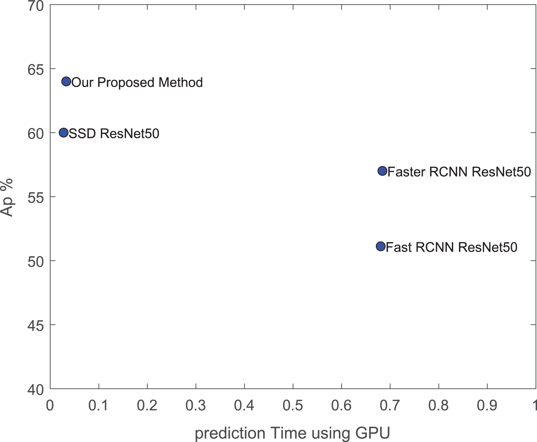
From this experiment, We have noticed that both fast and faster RCNN consumed higher training and testing time than all SSD architectures. The previous saliency SSD architecture in the literature based on two VGG networks requires 45 M parameters which required more training and testing time (Du et al., 2019). On the other hand, it is important to compare the architecture speed relative to its detection performance. As shown in Fig. 17, our proposed method has achieved the best AP value with a low prediction time for our detection target.
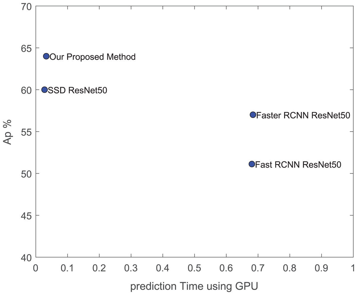
Figure 17: AP performance vs. prediction time using our GPU.
Conclusions
This study proposes a building detection algorithm based on the development of the SSD algorithm for a new buildings dataset in the desert environment. First, a data augmentation stage was applied to increase the detection results accuracy. We have investigated the performance of different pre-trained networks. We have proven that the ResNet50 network has more discriminated features for our building detection target. We have also compared the SSD detector with the previous methods. The SSD detector with ResNet50 has achieved the best performance compared to the previous methods. On the other hand, we have developed the SSD backbone using a visual saliency attention mechanism. We have investigated two approaches for the saliency attention fusion model. Our second proposed approach has achieved better performance. Moreover, we have investigated the fusion function between spatial and saliency features maps. We have proven that the addition fusion function for our detection target has a better detection performance. The saliency visual attention has improved all evaluation metrics for SSD ResNet50 architecture. In future work, there is still a challenge to increase the system performance evaluation metrics. The dataset size can be increased to increase the system performance. The building detection task can be discussed from a semantic segmentation point of view. A saliency attention layer improvement can increase the detection accuracy results. The saliency visual attention mechanism can be fused with more detectors such as YOLO detectors. Our detection algorithm can be generalized to detect other targets in remote sensing applications.