
Interpretable four-class brain tumor MRI classification using a fine-tuned ResNet50
- Published
- Accepted
- Received
- Academic Editor
- Nicole Nogoy
- Subject Areas
- Bioengineering, Bioinformatics, Neurology, Science and Medical Education, Data Science
- Keywords
- MRI, LLM, ResNet50, Brain tumor, Grad-CAM++
- Copyright
- © 2026 Veneri
- Licence
- This is an open access article distributed under the terms of the Creative Commons Attribution License, which permits unrestricted use, distribution, reproduction and adaptation in any medium and for any purpose provided that it is properly attributed. For attribution, the original author(s), title, publication source (PeerJ Computer Science) and either DOI or URL of the article must be cited.
- Cite this article
- 2026. Interpretable four-class brain tumor MRI classification using a fine-tuned ResNet50. PeerJ Computer Science 12:e3643 https://doi.org/10.7717/peerj-cs.3643
Abstract
Background
Automated classification of brain tumors from magnetic resonance imaging (MRI) can support radiologists and accelerate treatment planning. Public benchmark datasets enable rapid prototyping but require rigorous evaluation and transparent reporting.
Methods
The publicly available Kaggle Brain Tumor MRI dataset (DOI: 10.34740/kaggle/dsv/2645886) comprising 7,023 contrast-enhanced, T1-weighted axial slices labeled as glioma, meningioma, pituitary tumor or no-tumor was used. After removing corrupted images and applying extensive augmentation, a convolutional neural network was trained via transfer learning. A Residual Network 50 (ResNet50) backbone pretrained on ImageNet was fine-tuned in a three-phase schedule: (i) frozen feature training of custom classifier layers, (ii) partial unfreezing with a reduced learning rate and (iii) full fine-tuning of all layers. Regularization strategies included dropout, Gaussian noise, L2 weight decay and label smoothing. Performance was evaluated on a held-out test set (n = 1,205) using accuracy, precision, recall, F1-score and confusion matrix analysis. Model interpretability was assessed with Grad-CAM++ heatmaps.
Results
The proposed model achieved 96.67% overall accuracy and a macro-averaged F1-score of 0.9658 on the unseen test set. Per-class recall ranged from 0.94 (meningioma) to 0.99 (pituitary). Training and validation curves indicated minimal overfitting, while Grad-CAM++ visualizations suggested that salient regions generally corresponded to tumor locations rather than background artifacts.
Discussion
These results demonstrate that a carefully regularized, fine-tuned ResNet50 provides a strong baseline for four-class brain tumor classification.
Limitations
Despite aggregating three subdatasets, the Kaggle corpus remains limited in diversity: all images correspond to axial, contrast-enhanced T1-weighted scans, and metadata on scanner type or acquisition protocol is unavailable. However, external clinical validation was not performed.
Future work
Directions include evaluation under domain-shift, validation on multi-institutional cohorts, extension to volumetric 3D models, and exploration of lightweight architectures for real-time deployment.
Conclusions
This work provides a reproducible baseline for interpretable brain tumor MRI classification, highlighting both the promise and current limitations of deep learning approaches prior to clinical validation.
Introduction
Brain tumors remain a major source of morbidity and mortality worldwide. Early diagnosis and subtype differentiation—particularly among glioma, meningioma and pituitary adenoma—are critical for guiding surgical resection strategies and adjuvant therapy. Magnetic resonance imaging (MRI) is the modality of choice because of its superior soft-tissue contrast; however, manual interpretation is labor-intensive and subject to interobserver variability.
Deep learning, particularly convolutional neural networks (CNNs), has transformed computer-aided diagnosis in radiology. Transfer learning from models pretrained on large natural-image corpora enables robust feature extraction even with limited medical data, as demonstrated by Wang, Wang & Zhang (2024). Several groups have applied Residual Network (ResNet)-based models to brain tumor MRI. Sharma et al. (2023) compared a custom CNN, Visual Geometry Group-16 (VGG) and Residual Network 50 (ResNet50) on a four-class MRI dataset derived from Kaggle and reported test accuracy around 95%, using a single random train-test split without cross-validation, ablation or interpretability analysis. Mohamed Mustafa et al. (2024) combined ResNet50 with Gradient-wighted Class Activation Mapping (Grad-CAM) on T1-weighted MRI and achieved 98.52% accuracy for tumor detection, focusing on binary labels (tumor vs. no-tumor) and qualitative saliency maps. Han et al. (2025) studied VGG16, ResNet50 and EfficientNet with Local Interpretable Model-agnostic Explanations (LIME) and Grad-CAM and showed that different backbones attend to different regions, but their work targeted relative architecture comparison rather than a rigorously evaluated ResNet50 baseline.
Overall, ResNet-based MRI classification studies report strong headline performance but often rely on single data splits, limited reporting of augmentation and regularization, and only illustrative Grad-CAM visualizations. Few works provide open, end-to-end pipelines with detailed error analysis on the widely used Kaggle four-class dataset.
This work presents an end-to-end framework that fine-tunes a ResNet50 backbone with modern regularization and provides visual explanations based on Grad-CAM++, which has been shown to improve upon Grad-CAM (Chattopadhyay et al., 2018). This work makes three main contributions to the literature on ResNet-based brain tumor MRI classification:
-
1.
Development of a fully documented ResNet50 pipeline on the popular four-class Kaggle dataset, with detailed reporting of augmentation and regularization.
-
2.
Execution of a rigorous evaluation including stratified 5-fold cross-validation, ablation of key design choices and calibration analysis.
-
3.
Performance of a structured Grad-CAM++ error analysis on no-tumor slices, with open code and model weights to facilitate reuse.
Materials and Methods
Dataset acquisition and preprocessing
The study utilized the open Brain Tumor MRI dataset (Msoud, 2021; Kaggle: DOI: 10.34740/kaggle/dsv/2645886, license Creative Commons Zero (CC0): Public Domain), containing 5,712 training and 1,311 testing slices. Image integrity was verified with the Python Imaging Library, and duplicate images were removed via Message Digest 5 (MD5) hashing. The final corpus comprised 6,726 unique JPG images divided into training (4,418), validation (1,103) and testing (1,205) sets. As the Kaggle dataset already incorporates images from the Figshare repository (Cheng, 2017; DOI: 10.6084/m9.figshare.1512427.v8), only Kaggle was retained to prevent duplication and potential data leakage.
Data licensing and ethical compliance
The dataset is released under a CC0 license, permitting unrestricted reuse, modification, and redistribution. All images are fully anonymized and released for research purposes; therefore, no institutional review board (IRB) approval was required.
Data augmentation
Augmentation was implemented via Keras’ ImageDataGenerator and included random rotations (±25°), horizontal flips, zoom (0–20%), brightness shifts (0.6–1.4), width/height shifts (±10%), shearing (±0.2), and channel shifts (±10). Augmented samples were reflected at borders to avoid artifacts. The augmentation ranges were selected based on two criteria:
-
1.
maintaining clinically plausible variability.
-
2.
introducing sufficient geometric and photometric diversity to counteract overfitting in a relatively homogeneous dataset.
A rotation of ±25° approximates variability in head tilt encountered in routine MRI acquisitions while avoiding unrealistic anatomical distortion. Shear distortions (±0.2) and width/height shifts (±10%) emulate differences in slice angulation and patient positioning. Channel shifts up to 10 simulate the small brightness fluctuations that commonly arise from differences in scanners, coils or calibration settings, without altering anatomical content.
Together, these parameters balance realism with sufficient variability to improve generalization without creating anatomically implausible inputs.
Augmentation was applied online at training time, so no augmented samples were stored on disk. The training split contained n_train = 4,418 samples. Steps per epoch were set to ceil(n_train/batch_size), where ceil(a/b) = (a + b – 1) // b. Therefore, phase 1 (batch size 32) used 139 steps per epoch, yielding 4,448 augmented samples per epoch and phase 2 (batch size 16) used 277 steps per epoch, yielding 4,432 augmented samples per epoch. Since these totals slightly exceed n_train, some training instances are repeated within an epoch, each time receiving an independent random transform.
Across 29 total epochs (18 head-training and 11 fine-tuning), the model processed approximately 128,816 augmented training samples.
Model architecture
ResNet50 was selected for its robust architecture, strong generalization ability and availability of ImageNet-pretrained weights. The convolutional base (weights = “imagenet”, include_top = False) accepted 224 × 224 × 3 inputs, followed by:
GlobalAveragePooling2D
GaussianNoise (0.10)
Dense (512, Rectified Linear Unit (ReLU), kernel_regularizer = L2 1e4)
Dropout (0.5)
GaussianNoise (0.05)
Dense (128, ReLU, kernel_regularizer = L2 1e4)
Dropout (0.5)
Dense (4, softmax)
GaussianNoise injects zero-mean noise into feature activations during training. The parameter σ denotes the noise standard deviation in activation units at the layer output (here applied after global average pooling with σ = 0.10 and after dropout with σ = 0.05). Since noise is not applied to raw pixel intensities, conventional MRI acquisition signal-to-noise ration (SNR) is not applicable. Instead, this study reports a feature-space SNR estimated at the input of each GaussianNoise layer. For signal activations s and injected noise n ~ N (0, σ2), SNR is defined as Var(s)/σ2 and SNR(dB) = 10·log10(Var(s)/σ2), where Var(s) is the mean variance across activation channels computed over mini-batches from the training split without augmentation. Feature-space SNR is reported to quantify the effective strength of activation noise; this calculation does not by itself determine an optimal σ.
Prior work in medical imaging has reported that CNNs can remain stable under synthetic perturbations that do not directly model acquisition noise (Buddenkotte & Buchert, 2024); here, GaussianNoise is used as a regularizer to improve generalization and calibration rather than to emulate MRI noise.
The final model contained 24,702,980 trainable parameters, occupying ~47 MB in float16 checkpoints (~94 MB in float32).
Baseline architecture (VGG16)
To contextualize performance, a VGG16 backbone was trained under identical preprocessing, augmentation, class weighting, input size (224 × 224), loss, optimizer family, label smoothing and evaluation protocol as ResNet50. Training followed the same two-phase schedule: (I) frozen-backbone training of the classification head and (ii) partial unfreezing with a reduced learning rate. VGG16 used ImageNet-pretrained weights (include_top = False), global average pooling and the same classification head as ResNet50. Performance was measured on the fixed test set and through a 5-fold cross-validation on the complete training pool, reporting accuracy, macro-precision, macro-recall and macro-F1 (mean ± standard deviation (SD)).
Training protocol
Training followed a three-phase schedule:
Phase 1: classifier-head training for 18 epochs using Adaptive Moment Estimation (Adam) (learning_rate = 1 × 10⁻⁴), batch size = 32.
Phase 2: gradual unfreezing of ResNet layers. The last 30 layers (excluding BatchNorm) fine-tuned for three epochs with AdamW (learning_rate = 3 × 10⁻⁵).
Phase 3: all layers were unfrozen and training continued for eight epochs with AdamW and polynomial decay (initial_learning_rate = 1 × 10⁻⁵), batch size = 16.
Mixed-precision (float16) was enabled. Validation performance was monitored with EarlyStopping (patience = 8) to prevent overfitting (Mohamed Mustafa et al., 2024), ReduceLROnPlateau (factor = 0.5), and ModelCheckpoint. Class weights were computed with scikit-learn to mitigate class imbalance. Training was performed on a single NVIDIA RTX 5000 Ada graphics processing unit (GPU) with 32 GB of Random-access memory (RAM). Software environment: Ubuntu (Windows Subsystem for Linux (WSL)), Python 3.10, TensorFlow 2.16.1, with corresponding CUDA and cuDNN versions.
Runtime analysis
Inference time per image was measured using the trained ResNet50 model on an NVIDIA RTX 5000 Ada GPU. Timing was averaged over 500 predictions on unseen test images, excluding the first prediction (which includes model loading into GPU memory). Reported values therefore represent steady-state inference performance, relevant for clinical workflow deployment.
Cross-validation design
To assess robustness, a full 5-fold stratified cross-validation was performed across the complete training pool (n = 5,521). The test set was held out entirely and remained unseen throughout all stages of training and model selection.
The training split was divided into five folds of equal size and preserved class balance. For each fold i, the model was:
-
1.
Initialized from ImageNet weights.
-
2.
Trained from scratch on the union of the remaining four folds (Dj).
-
3.
Validated on the held-out fold (Di), which was never used during training or augmentation.
Performance metrics (accuracy, precision, recall, F1-score) were computed for each fold and finally averaged to obtain mean ± SD.
The external test set was kept completely unseen and was not involved in the cross-validation procedure.
Evaluation design and metrics
Model effectiveness was evaluated using a stratified 65:15:20 split, preserving representative class proportions. The test set (n = 1,205) remained untouched until final evaluation. Performance metrics included accuracy, precision, recall, F1-score and confusion matrices, computed per class and macro-averaged. Macro-averaging was preferred over micro-averaging to ensure that performance degradation in minority classes (e.g., meningioma, no-tumor) was not obscured by dominant classes.
Selection method
ResNet50 was chosen based on its proven success in medical imaging tasks and availability of robust pretrained weights. Regularization strategies (dropout, Gaussian noise, L2 weight decay, label smoothing) were selected through preliminary experimentation and supported by literature.
Interpretability
The public dataset provides 2D JPG slices without DICOM orientation metadata. For visualization only, displayed example slices were reoriented into consistent view conventions (axial: anterior up; sagittal: anterior left; coronal: superior up). Left-right laterality is not asserted. Grad-CAM++ heatmaps were generated with tf-keras-vis and qualitatively inspected on correctly and incorrectly classified examples. Representative cases are presented in the Results.
Code repository
All code, trained weights, and complete instructions for reproducibility are publicly available on GitHub at https://github.com/pietroveneri/Brain-Tumor-MRI. Additional archival is provided via Zenodo (DOI: 10.5281/zenodo.17968706).
Results
The study evaluated a fine-tuned ResNet50 for four-class brain tumor classification using the Kaggle Brain Tumor MRI dataset (n = 7,023; glioma, meningioma, pituitary, no-tumor). Images were split 65:15:20 into training (n = 4,418), validation (n = 1,103), and testing (n = 1,205).
Training and validation
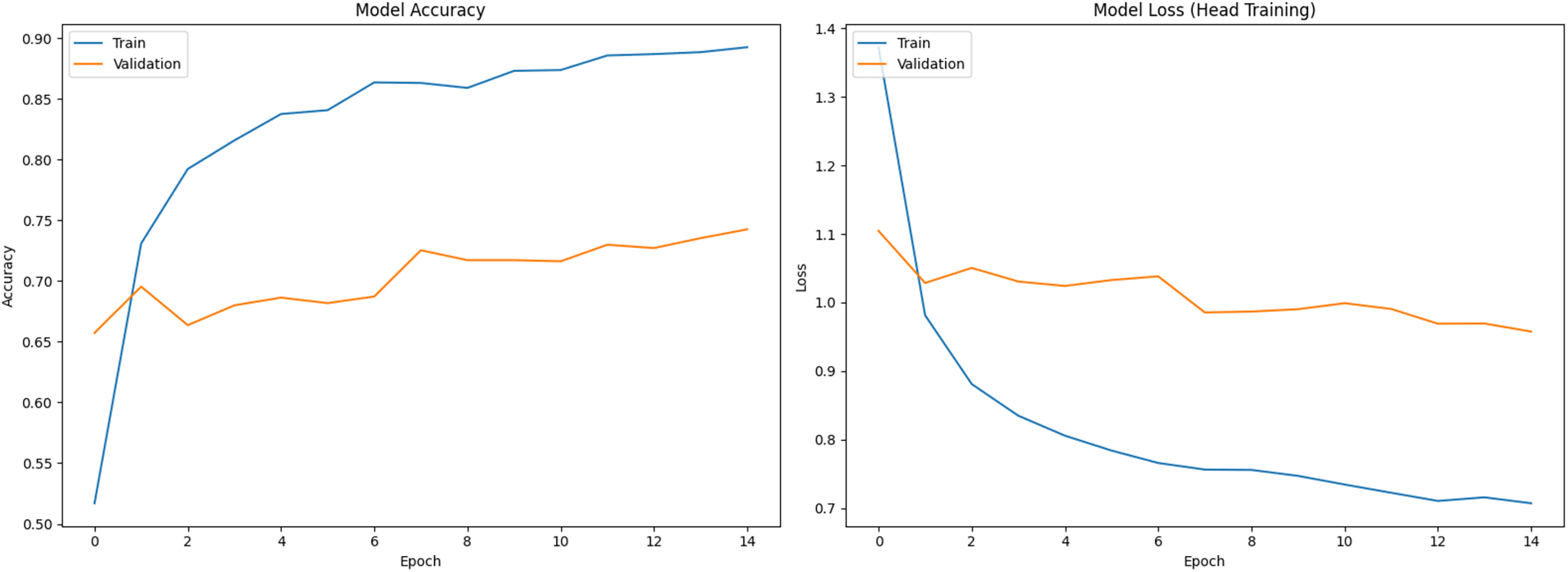
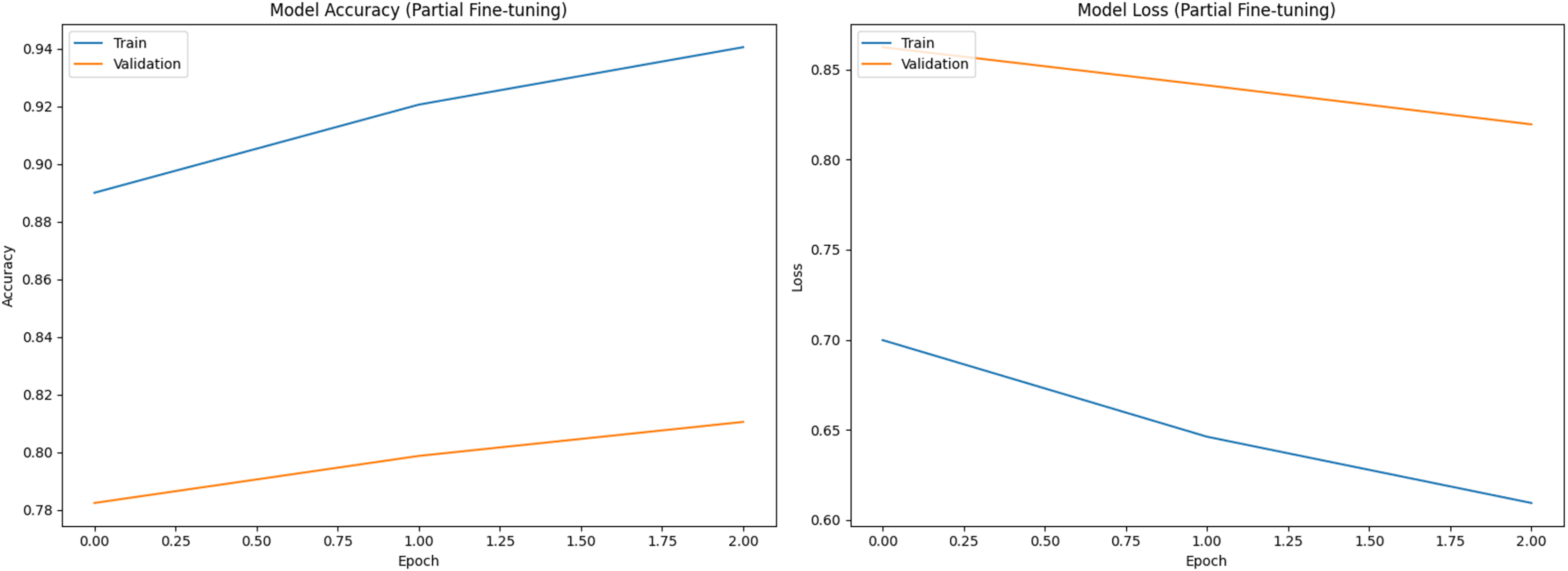
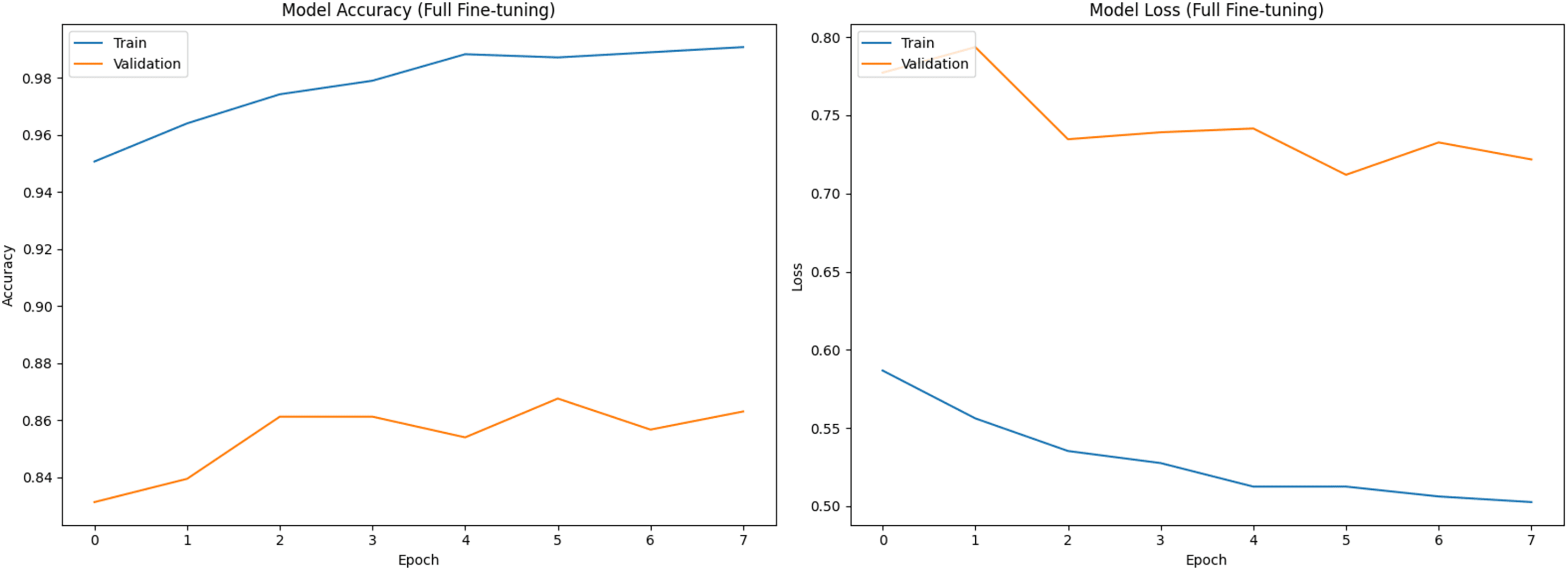
Figure 1 shows training (blue) and validation (orange) curves during phase 1 (classifier head training), with accuracy on the left and loss on the right. Figures 2 and 3 illustrate analogous curves for the partial and full fine-tuning. Convergence was stable, with minimal evidence of overfitting.
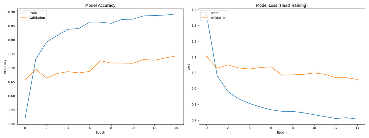
Figure 1: Training and validation curves during initial classifier training phase (Accuracy and Loss).
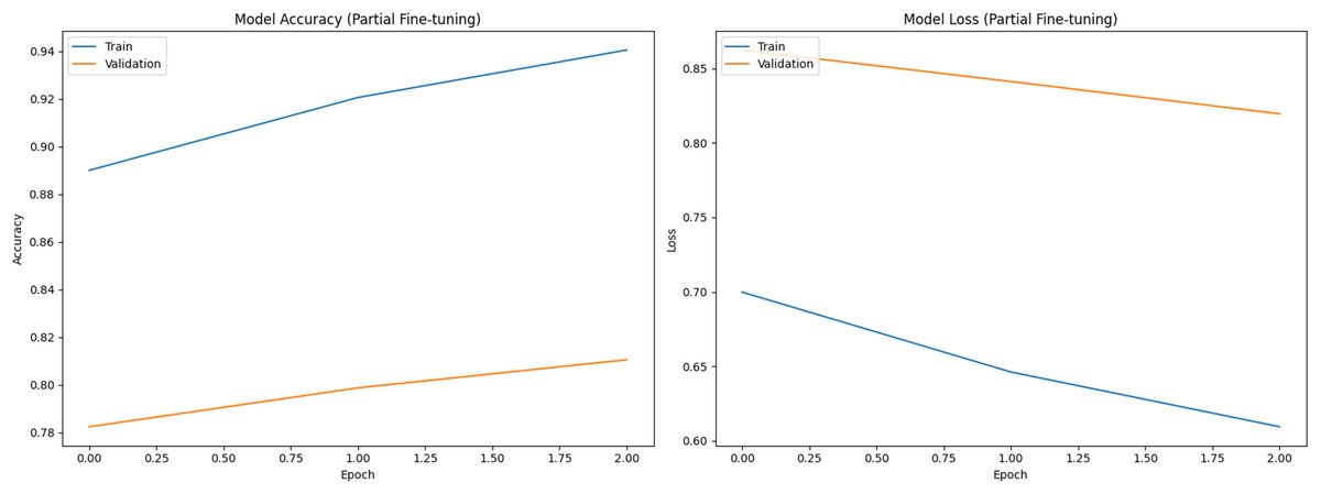
Figure 2: Training and validation curves during partial fine-tuning phase (Accuracy and Loss).
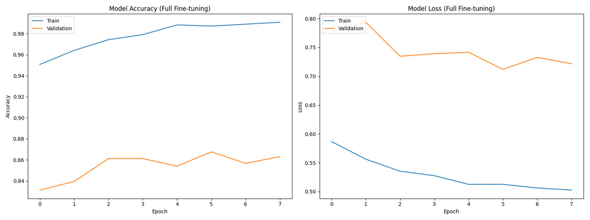
Figure 3: Training and validation curves during full fine-tuning phase (Accuracy and Loss).
Feature-space of GaussianNoise
Using 50 mini-batches from the training split without augmentation, the activation variance at the input of the first GaussianNoise layer (after global average pooling) was 0.0512 ± 0.0256, yielding SNR = 6.64 ± 1.92 dB for σ = 0.10. For the second GaussianNoise layer (after dropout1) the activation variance was 0.1076 ± 0.0174, yielding SNR = 16.29 ± 0.60 dB for σ = 0.05. σ values were selected a priori as mild regularizers (σ = 0.10 and 0.05) and retained because they improved calibration without degrading macro-F1 on the test set.
Test set performance
Across three independent runs, ResNet50 achieved a mean accuracy of 96.67 ± 0.57% (95% CI [0.960–0.973]). Table 1 shows per-class performance metrics and Fig. 4 presents the confusion matrix from a representative run, showing increased confusion among meningiomas.
| Classes | Precision | Recall | F-score |
|---|---|---|---|
| G | 0.9767 ± 0.0057 | 0.9667 ± 0.0012 | 0.9733 ± 0.0057 |
| M | 0.9467 ± 0.0012 | 0.9400 ± 0.0100 | 0.9400 ± 0.0100 |
| NT | 0.9800 ± 0.0000 | 0.9767 ± 0.0057 | 0.9767 ± 0.0057 |
| P | 0.9667 ± 0.0057 | 0.9867 ± 0.0058 | 0.9733 ± 0.0057 |
| Macro avg | 0.9675 ± 0.0149 | 0.9675 ± 0.0200 | 0.9658 ± 0.0172 |
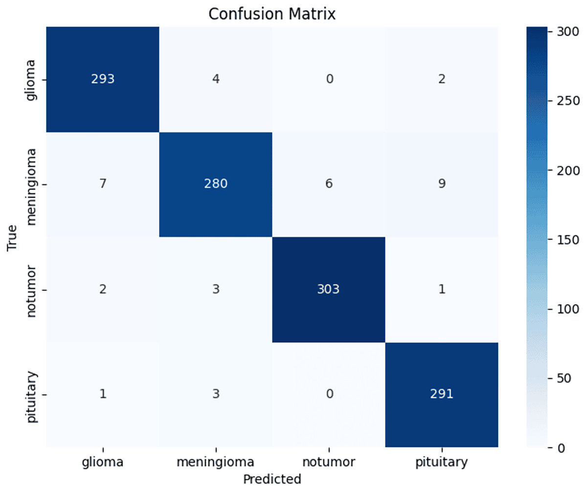
Figure 4: Confusion matrix.
Confusion matrix from a representative ResNet50 test run, showing per-class distribution of true and misclassified cases.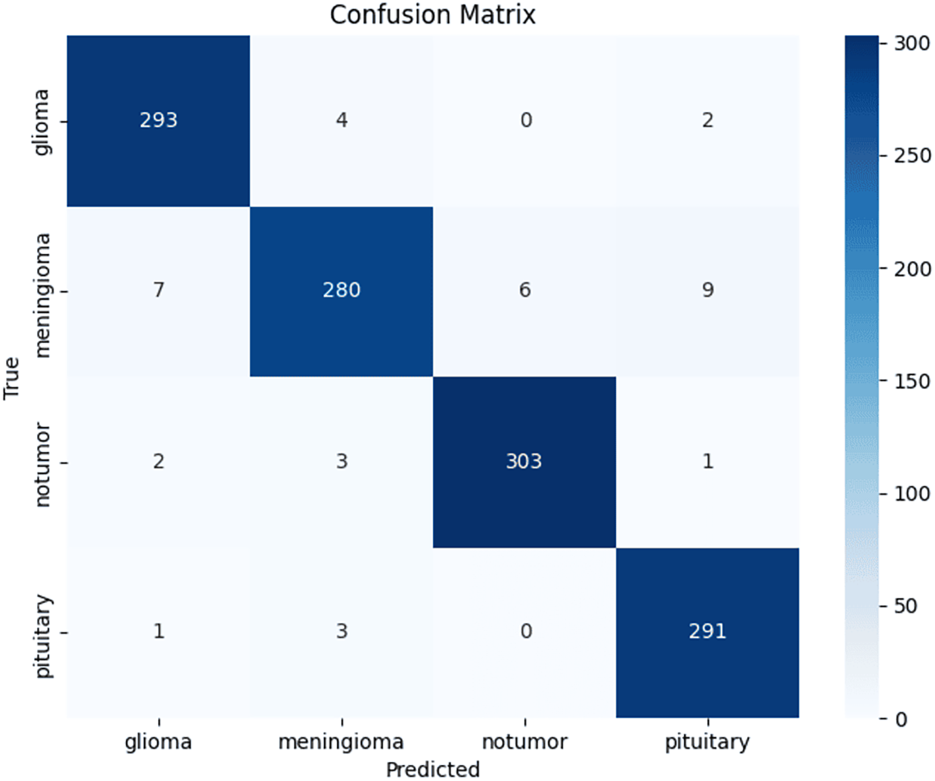
Cross-validation results
Stratified 5-fold cross-validation on the training pool yielded a mean macro-averaged F1-score of 0.9524 ± 0.0053, with values ranging from 0.9465 to 0.9575 across folds. Table 2 summarizes mean and standard deviation of precision, recall and F1-score per fold, confirming robustness to dataset partitioning.
| Macro-Precision | Macro-Recall | Macro-F1-score | |
|---|---|---|---|
| Fold 1 | 0.9479 | 0.9477 | 0.9465 |
| Fold 2 | 0.9527 | 0.9576 | 0.9575 |
| Fold 3 | 0.9552 | 0.9529 | 0.9532 |
| Fold 4 | 0.9494 | 0.9475 | 0.9474 |
| Fold 5 | 0.9594 | 0.9584 | 0.9574 |
| Mean ± SD | 0.9529 ± 0.0046 | 0.9528 ± 0.0052 | 0.9524 ± 0.0053 |
Baseline comparison
A VGG16 baseline was trained under identical augmentation, preprocessing, fine-tuning schedule and evaluation protocol. Table 3 reports the direct comparison between architectures. Both models achieved competitive performance, but ResNet50 consistently reached higher recall (0.9675 ± 0.0200) than VGG16 (0.9666 ± 0.0288) and exhibited lower variability across runs. Table 4 reports VGG16’s per-class performance metrics. VGG16 showed stronger F1-score for no-tumors, whereas ResNet50 achieved higher precision and F1-score in glioma tumors. Overall, both architectures generalized well, but ResNet50 demonstrated greater stability.
| Model | Macro-Precision | Macro-Recall | Macro-F1 |
|---|---|---|---|
| ResNet50 | 0.9675 ± 0.0149 | 0.9675 ± 0.0200 | 0.9658 ± 0.0172 |
| VGG16 | 0.9674 ± 0.0133 | 0.9666 ± 0.0288 | 0.9658 ± 0.0185 |
| Classes | Precision | Recall | F-Score |
|---|---|---|---|
| G | 0.9733 ± 0.0057 | 0.9667 ± 0.0058 | 0.9667 ± 0.0058 |
| M | 0.9600 ± 0.0000 | 0.9267 ± 0.0230 | 0.9400 ± 0.0100 |
| NT | 0.9833 ± 0.0058 | 0.9800 ± 0.0000 | 0.9833 ± 0.0058 |
| P | 0.9533 ± 0.0115 | 0.9933 ± 0.0058 | 0.9733 ± 0.0058 |
| Macro avg | 0.9674 ± 0.0133 | 0.9666 ± 0.0288 | 0.9658 ± 0.0185 |
Cross-validation comparison
Stratified five-fold cross-validation was performed on the training pool only, with the external test set excluded from fold generation, training and model selection. ResNet50 achieved macro-precision 0.9529 ± 0.0046, macro-recall 0.9528 ± 0.0052 and macro-F1 0.9524 ± 0.0053. VGG16 achieved macro-precision 0.9484 ± 0.0111, macro-recall 0.9567 ± 0.0126 and macro-F1 0.9468 ± 0.0124 (Table 5). VGG16 showed higher fold-to-fold variability across all metrics, with standard deviations approximately 2 times larger than ResNet50 on most macro metrics, indicating lower stability.
| Model | Accuracy | Macro-Precision | Macro-Recall | Macro-F1 |
|---|---|---|---|---|
| ResNet50 | 0.9528 ± 0.0052 | 0.9529 ± 0.0046 | 0.9528 ± 0.0052 | 0.9524 ± 0.0053 |
| VGG16 | 0.9567 ± 0.0126 | 0.9484 ± 0.0111 | 0.9567 ± 0.0126 | 0.9468 ± 0.0124 |
Ablation study
Table 6 reports six variants. Removing label smoothing produced a small drop in performance (accuracy 0.9602, macro-F1 0.96) and reduced meningioma recall to 0.94. Removing GaussianNoise increased accuracy to 0.9701 but raised test loss to 0.50, indicating weaker probability calibration. Augmentation was the primary driver of generalization gains. Turning off all augmentations caused severe overfitting, with training accuracy reaching 1.00 while validation plateaued at 0.85 and test accuracy dropped to 0.9477 (macro-F1 0.95). This yields a train-validation gap of 0.15 and a train-test gap of 0.0523. Removing spatial transforms produced the same failure patterns (test accuracy 0.9494, meningioma recall 0.88). Removing photometric transforms preserved test accuracy (0.9701) but widened the train-validation gap (0.99 vs. 0.87) and increased test loss (0.50), consistent with the model’s reduced ability to handle intensity variation.
| Variant | Train Acc. | Val Acc. | Accuracy | Macro-F1 | Test Loss | Meningioma recall | Notes |
|---|---|---|---|---|---|---|---|
| Full pipeline (baseline) | 0.96 | 0.88 | 0.9667 | 0.9658 | 0.28 | 0.94 | Reference |
| No Gaussian Noise | 0.99 | 0.87 | 0.9701 | 0.97 | 0.50 | 0.93 | Higher loss |
| No label smoothing | 0.99 | 0.87 | 0.9602 | 0.96 | 0.22 | 0.94 | Slightly weaker generalization |
| All augmentations OFF | 1.00 | 0.85 | 0.9477 | 0.95 | 0.53 | 0.88 | Severe overfitting |
| No spatial (photometric only) | 0.99 | 0.85 | 0.9494 | 0.95 | 0.53 | 0.88 | Strong overfitting |
| No photometric (spatial only) | 0.99 | 0.87 | 0.9701 | 0.97 | 0.50 | 0.89 | Wider train-val gap |
Inference time
Mean inference time was ~130 ms per image on GPU after initialization. The first prediction was slower (~2 s) due to model loading, but this cost occurs only once per session. At steady state, the model processes ~8 images per second, supporting feasibility for near real-time clinical workflows.
Grad-CAM++ analysis
Representative heatmaps showed activation hotspots aligning with tumor regions in true-positive (Figs. 5, 6).
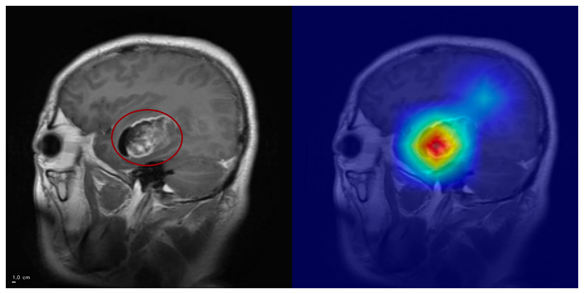
Figure 5: Grad-CAM++ visualization: correct glioma classification.
The tumor mass (circled, left) is highlighted by Grad-CAM++ (right), demonstrating strong alignment between model attention and the lesion. Anterior is on the left and superior is up. Left–right laterality is not reported because the public JPG dataset lacks DICOM orientation metadata. Scale bar: 1 cm (approximate, based on resampled voxel spacing).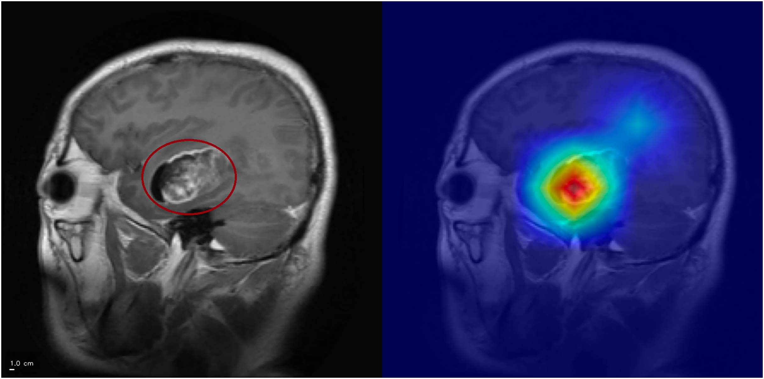
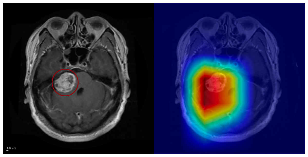
Figure 6: Grad-CAM++ visualization: correct meningioma classification.
The tumor mass (circled, left) is highlighted by Grad-CAM++ (right), although attention also extends into surrounding tissue. This overactivation illustrates that the model may attend beyond the lesion boundaries. Anterior is at the top and posterior is at the bottom. Left–right laterality is not reported because the public JPG dataset lacks DICOM orientation metadata. Scale bar: 1 cm (approximate, based on resampled voxel spacing).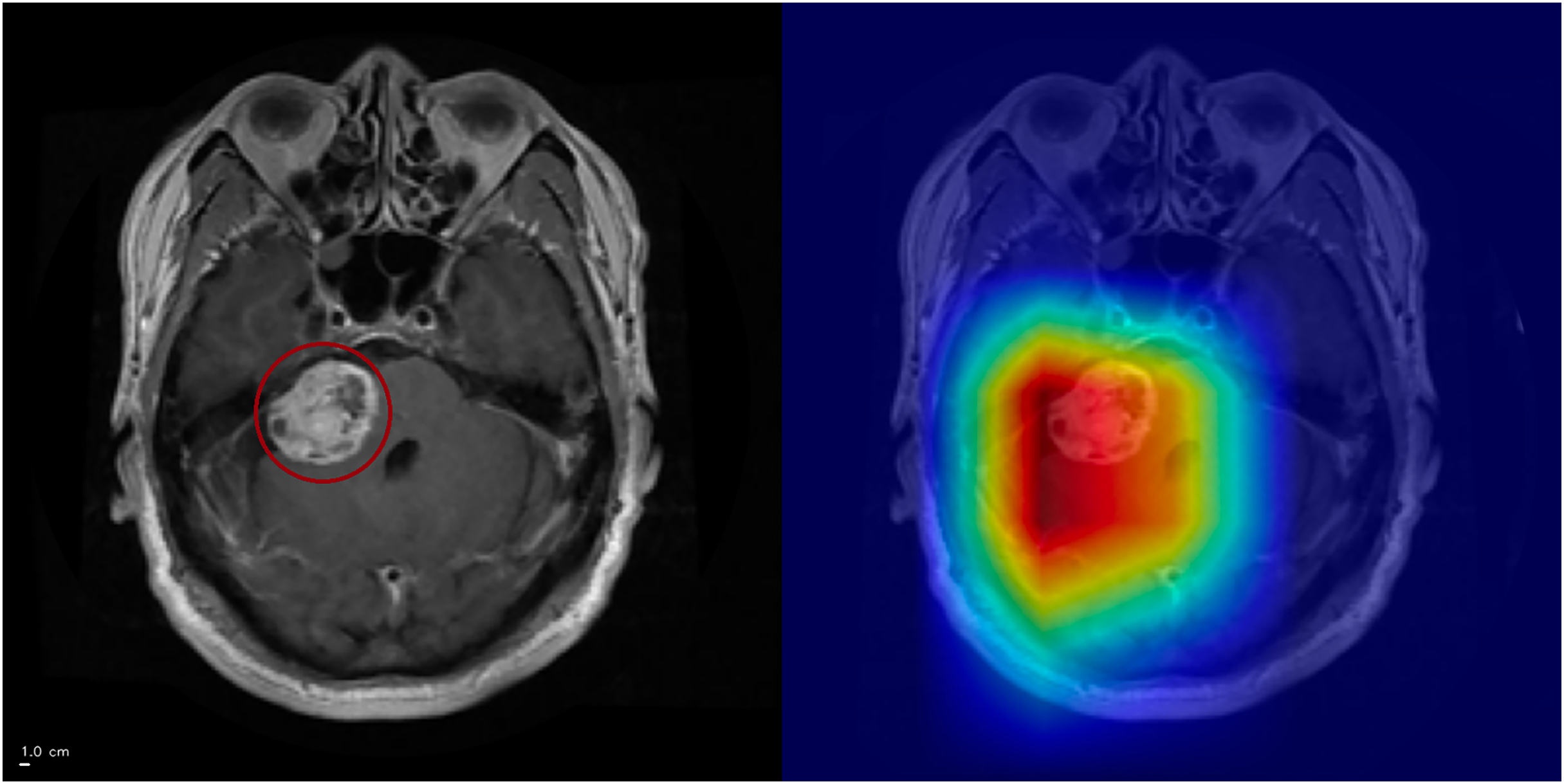
Error analysis was performed exclusively on the held-out test (n = 1,205). Across three independent runs, the model produced 4-5 false positives per run. While the specific misclassified slices varied between runs, the qualitative failure patterns recurred:
-
1.
Normal cortical or subcortical tissue misinterpreted as pathology.
-
2.
Cerebrospinal Fluid (CSF)-related regions receiving attention (Fig. 7).
-
3.
Diffuse, low-contrast attention without a clear anatomical correlate.
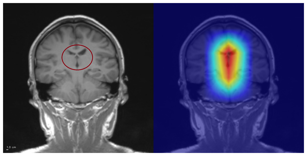
Figure 7: Example of CSF-related false positive activation.
The Grad-CAM++ heatmap (right) highlights spurious attention in the interhemispheric fissure (circled, left), a cerebrospinal fluid (CSF) region. Such activations illustrate how the model may misinterpret CSF-related structures as pathological features, leading to false positives. Superior is up and inferior is down. Left–right laterality is not reported because the public JPG dataset lacks DICOM orientation metadata. Scale bar: 1 cm (approximate, based on resampled voxel spacing).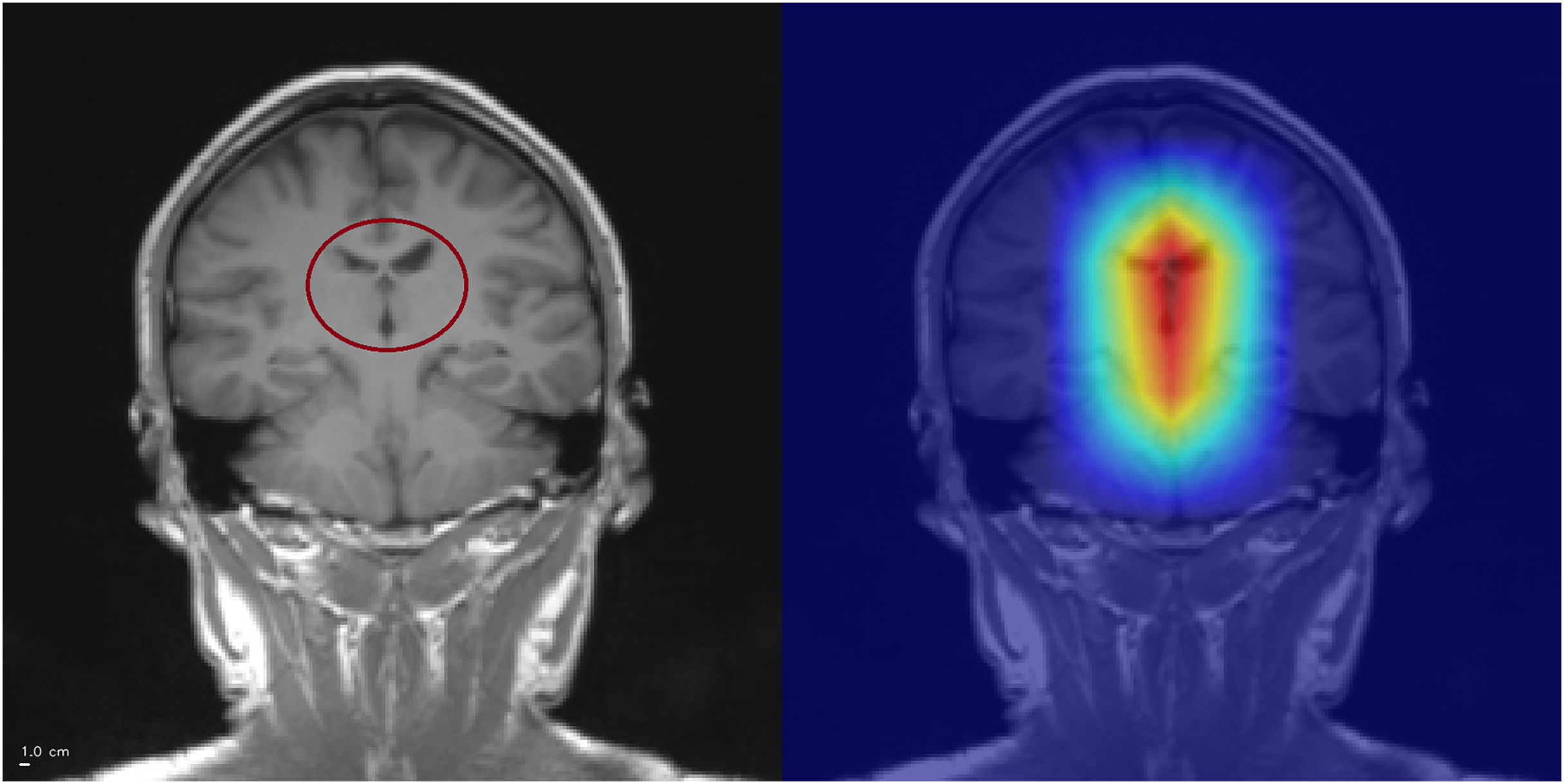
CSF-related false activations represented a minority of false positives and did not dominate the error profile. Diffuse, low-contrast saliency without a clear anatomical correlate was observed in a subset of false positives, indicating reduced reliability of the attribution map in some incorrect predictions rather than a consistent anatomical confounder. This reflects a known limitation of post-hoc attribution methods rather than systematic model bias.
Rarely, high-confidence predictions (≥94% probability) lacked clear hotspots (Fig. 8). Examination of earlier convolutional layers revealed weak but spatially coherent activations tracing tumor-like regions, suggesting saliency reliability may be layer-dependent.
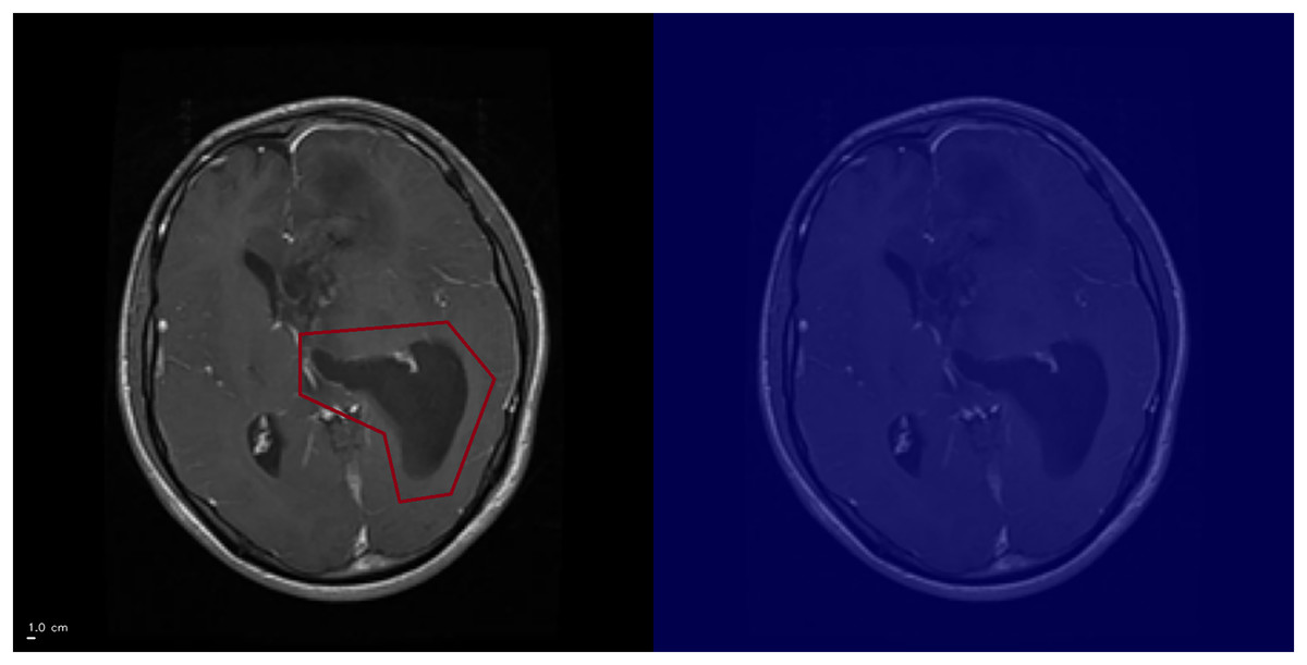
Figure 8: Grad-CAM++ visualization: example of high-confidence glioma prediction without clear activation.
The ground-truth tumor region is outlined (left), but Grad-CAM++ fails to generate a corresponding activation (right). This illustrates a limitation of Grad-CAM++, where saliency maps may not reliably capture pathological features. Anterior is at the top and posterior is at the bottom. Left–right laterality is not reported because the public JPG dataset lacks DICOM orientation metadata. Scale bar: 1 cm (approximate, based on resampled voxel spacing).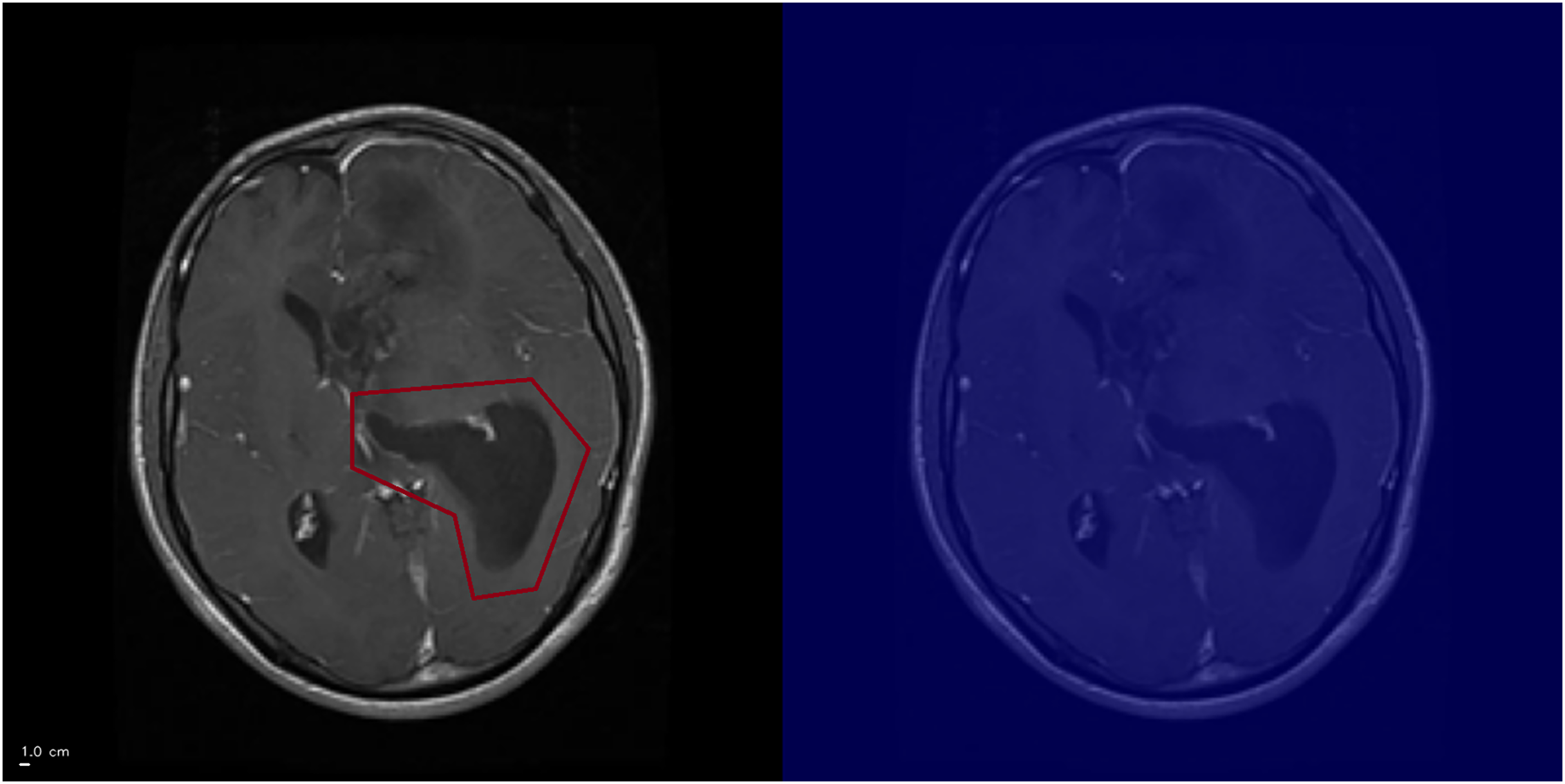
Discussion
Main outcomes
Three-phase fine-tuning of ResNet50 achieved 96.67% accuracy, comparable to ensemble methods but with fewer epochs and lower computational cost. Regularization strategies mitigated overfitting, while Grad-CAM++ demonstrated biologically plausible features.
Comparison with literature
ResNet-based pipelines dominate recent work on brain tumor MRI. Sharma et al. (2023) reported 94.83% accuracy on 4,225 slices with a ResNet50 backbone, relying on a single split and lacking interpretability assessment. Mohamed Mustafa et al. (2024) used ResNet50 with Grad-CAM on a Kaggle-derived dataset and achieved 98.52% accuracy for tumor detection again with binary labels and no systematic ablation or cross-validation. In the present study, a fine-tuned ResNet50 reaches 96.67% accuracy and macro-F1 0.9658 on a fixed held-out test and is evaluated through full five-fold cross-validation, ablation of regularization and augmentation, and structured analysis of Grad-CAM++ failure modes on no-tumor slices. Compared with Sharma et al. (2023), the pipeline attains higher accuracy with fewer epochs and shorter per-slice inference time, while also reporting calibration and feature-space SNR for GaussianNoise layers. Han et al. (2025) highlighted that VGG16, ResNet50 and EfficientNet produce different attribution patterns. The present work complements that study by treating ResNet50 as a single, well-characterized backbone and by providing a reproducible reference implementation on the popular Kaggle dataset.
Interpretation of baselines
VGG16 achieved performance close to ResNet50 but with higher run-to-run variability. ResNet50 offered greater stability and precision for glioma and meningioma, justifying its selection as the preferred backbone. This is consistent with prior evidence that backbone choice influences both performance stability and post-hoc interpretability behavior (Han et al., 2025).
Cross-validation results
Stratified 5-fold cross-validation on the training pool showed stable performance across folds and lower fold-to-fold variability for ResNet50 than for VGG16, supporting robustness under resampling. Despite this, evaluation is still constrained to a single public dataset of 2D slices. External validation on independent, multi-institutional cohorts remains necessary to assess generalizability under domain shift.
Class-specific performance
Meningioma achieved the lowest recall rate, likely reflecting its biological heterogeneity—from small incidental lesions to large, highly vascularized tumors—posing challenges for generalization and motivating targeted improvements.
Ablation study
Label smoothing provided only marginal benefits. Gaussian noise did not enhance headline accuracy but improved probability calibration. Data augmentation was the dominant factor. Removing spatial transformations harmed generalization and meningioma recall, while removing photometric augmentations reduced robustness against acquisition variability. Turning off all augmentation caused severe overfitting, with training accuracy reaching 1.00 while validation and test performance dropped. This indicates strong dataset homogeneity and supports the interpretation that the network memorizes slice-specific patterns rather than learning robust tumor cues, a known limitation of 2D slice benchmarks curated from limited sources. Here, augmentation acts as a safeguard against shortcut learning, not only to increase accuracy. Without augmentation, Grad-CAM++ heatmaps can appear plausible even when decisions rely on brittle cues such as texture, contrast or background structure.
These findings reinforce consensus that augmentation is essential in medical imaging with limited dataset diversity.
Dataset and methodological limitations
Although the Kaggle dataset aggregates multiple sources, its diversity is limited: all images are axial, contrast-enhanced T1-weighted scans with no metadata on scanner type, acquisition protocol, or patient demographics. This constrains evaluation of domain shift. The use of 2D slices precludes modeling of cross-slice continuity. Interpretability was assessed qualitatively through Grad-CAM++ heatmaps; quantitative saliency validation (e.g., Dice or IoU overlap with tumor masks) was not possible due to the absence of voxel-level annotations. This limitation is dataset-driven rather than methodological. Future work should integrate datasets with segmentation masks to enable rigorous quantitative validation.
Error analysis and interpretability
False positives on no-tumor slices clustered into three qualitative patterns: attention on normal cortical or subcortical anatomy, CSF-adjacent attention, and diffuse low-contrast attention without a clear anatomical correlation. The diffuse pattern constituted the majority of false positives, indicating that the network at times assigns elevated attention to structurally normal regions. These activations showed no consistent anatomical pattern and were distributed across cortical and subcortical areas. CSF-related attention occurred in a minority of false positives but was not the dominant failure mode, suggesting that the model is not systematically biased toward ventricular or fissural regions.
Rare high confidence errors without clear saliency hotspots further illustrate the layer-dependence of Grad-CAM++: earlier convolutional layers often retained weakly localized responses, whereas the final layer occasionally failed to produce meaningful maps.
These observations highlight a key limitation of saliency methods. Attention maps can remain plausible even when predictions are incorrect and their reliability decreases when the model lacks multi-slice context or encounters ambiguous tissue patterns. This underscores the need for quantitative interpretability validation and for adopting additional regularization or multi-slice strategies to reduce structurally driven false positives.
Alternative post-hoc explainers such as LIME and SHapley Additive exPlanations (SHAP) offer complementary, model-agnostic insights but introduce substantial computational overhead. Recent evaluations (Narkhede, 2024) report that LIME requires the longest inference time per image but has modest memory usage, whereas SHAP exhibits intermediate runtime but significantly higher memory demand. Grad-CAM++ provides near real-time performance with minimal memory cost, which makes it suitable for large-scale medical imaging. Future work could integrate LIME or SHAP to complement Grad-CAM++ and strengthen interpretability assessment.
Deployment feasibility
Inference speed (~130 ms per image) supports near real-time clinical workflows. Optimization strategies such as pruning, quantization or lighter backbones (e.g., EfficientNet, ConvNeXt) could further reduce latency for clinical deployment.
Future work
Next steps include validation across institutions and scanners, extension to 3D volumes or slice sequences, neuroradiologist adjudication of Grad-CAM++ heatmaps, integration of uncertainty estimations and preprocessing strategies such as CSF masking or tissue-specific augmentation to further reduce these spurious activations. These will be essential for bridging research with clinical translation.
Conclusions
This study demonstrates that a transfer-learning pipeline based on ResNet50 with modern regularization and Grad-CAM++ achieves high accuracy and interpretable classification across four brain tumor categories using a widely adopted public MRI dataset. By releasing full code, trained weights and documentation, the work provides a reproducible and extensible baseline for future research in medical image analysis. Although not designed for clinical deployment, the results underscore the potential of interpretable deep learning to support radiological decision-making. For instance, Gao et al. (2022) showed that saliency-based assistance increased neuroradiologists’ diagnostic accuracy by over 10%. Building on such evidence, further advances in robustness and interpretability could help bridge the gap between research and translational application.
Several limitations remain. The study relied exclusively on publicly available, fully anonymized data, requiring no institutional ethics approval (EU GDPR Recital 26). No identifiable patient information was present in any image. Crucially, the model has not been clinically validated and is intended strictly for research purposes.