
SOSCNV: a stochastic outlier selection algorithm-based method for copy number variation detection using hybrid strategy
- Published
- Accepted
- Received
- Academic Editor
- Davide Chicco
- Subject Areas
- Computational Biology, Algorithms and Analysis of Algorithms, Data Mining and Machine Learning, Scientific Computing and Simulation
- Keywords
- Copy number variation, Stochastic outlier selection, Read depth, Split read, Tandem duplication
- Copyright
- © 2026 Du et al.
- Licence
- This is an open access article distributed under the terms of the Creative Commons Attribution License, which permits unrestricted use, distribution, reproduction and adaptation in any medium and for any purpose provided that it is properly attributed. For attribution, the original author(s), title, publication source (PeerJ Computer Science) and either DOI or URL of the article must be cited.
- Cite this article
- 2026. SOSCNV: a stochastic outlier selection algorithm-based method for copy number variation detection using hybrid strategy. PeerJ Computer Science 12:e3619 https://doi.org/10.7717/peerj-cs.3619
Abstract
Background
Copy number variation (CNV) refers to the duplication or deletion of DNA sequences in the genome. It plays an important role in organism development and disease occurrence.
Methods
Read-depth (RD)–based strategies are among the most widely used approaches for CNV detection; however, RD signals typically allow only approximate breakpoint localization. In contrast, split-read (SR) methods can provide much more precise breakpoint resolution. As a result, hybrid RD+SR strategies have become increasingly popular in recent CNV detection frameworks. Nevertheless, these hybrid methods still exhibit limitations, particularly in detecting CNVs of diverse lengths, where performance may degrade for very short or very long variants. A new CNV detection method called SOSCNV (Detection of Copy Number Variations based on Stochastic Outlier Selection) is proposed in this article. In order to enhance the recognition and processing ability of those difficult-to-detect areas, and also to make the detection of breakpoints more accurate, SOSCNV incorporates a two-stage segmentation technique. SOS algorithm is used to model the RD signal and Guanine and Cytosine (GC) content, and calculate the correlation between datasets to identify anomalous datasets. Compared with traditional RD+SR hybrid detection strategies, SOSCNV is better suited for identifying CNVs across a wide range of variant lengths and demonstrates stronger robustness under varying sequencing depths and tumor purities.
Results
After testing on 900 simulated datasets and four real datasets, and comparing with four existing CNV detection tools, experiments show that SOSCNV can significantly improve detection precision, recall and F1-score.
Introduction
In the genome, copy number variation (CNV) refers to the duplication or deletion of large DNA sequence segments in the genome (Li et al., 2020), CNV is of great significance for the occurrence and development of human health and diseases, and may also be related to the formation and development of tumors (Pös et al., 2021; Zhang et al., 2009). Therefore, developing an accurate and efficient detection method for cancer somatic CNV is of great significance for the early diagnosis and treatment of cancer (Freeman et al., 2006).
At present, the mainstream strategies for detecting CNV are divided into four categories (Zhang et al., 2019): (1) Read Depth (RD) (Kosugi et al., 2019), (2) Pair-end Mapping (PEM) (Hu et al., 2012), (3) Split Read (SR) (Ye et al., 2018), (4) de novo assembly (AS) (Paszkiewicz & Studholme, 2010). There are also algorithms that integrate the above strategies. In CNV detection, the strategy based on RD is currently one of the most widely used algorithms. According to this strategy, many CNV detection algorithms have been proposed, such as ReadDepth (Miller et al., 2011), RSICNV, CNV-IFTV (Yuan et al., 2019) and OTSUCNV (Xie et al., 2024). ReadDepth uses the preprocessed RD information to fit a negative binomial distribution model; RSICNV uses RD information and statistical models to analyze data, while CNV-IFTV infers gene copy numbers by analyzing the reordering information of DNA fragments, OTSUCNV employs an adaptive sequence segmentation algorithm combined with an OTSU-based prediction framework to detect CNV by analyzing characteristic signals. However, these tools cannot accurately identify the boundaries of CNV regions.
In addition, SR-based strategies have also been applied in the detection of CNV. This strategy identifies breakpoints with relatively high precision by directly locating partial alignments that overlap with breakpoints. Representative tools such as SplazerS (Emde et al., 2012) and SLOPE (Abel et al., 2010) utilize SR signals to achieve sensitive detection of small-scale variations. However, due to the short-read lengths of second-generation sequencing data, SR-based methods may encounter issues such as multiple alignments and missed detections when identifying larger variations or complex genomic regions.
Hybrid detection frameworks that integrate clustering and outlier-based strategies remain highly relevant and widely adopted across modern computing domains. For example, such approaches have been successfully applied in credit approval prediction and network intrusion detection, demonstrating strong adaptability and robustness in complex, noisy data environments (Dhahir, 2024; Setiadi et al., 2024). To further improve detection performance, more and more tools have attempted to integrate multiple strategies. Delly (Rausch et al., 2012) combines SR and PEM signals, while LUMPY (Layer et al., 2014) integrates RD, SR, and PEM strategies to achieve more robust structural variation detection. Such hybrid strategies can, to some extent, balance detection sensitivity and breakpoint accuracy. Although several hybrid RD and SR approaches such as LUMPY (Layer et al., 2014), TARDIS (Soylev et al., 2019), and OTSUCNV (Xie et al., 2024) have been widely used, they still exhibit notable limitations. These methods rely heavily on manually tuned parameters and lack true unsupervised adaptability, making their performance sensitive to sequencing noise and coverage fluctuations. Their breakpoint accuracy is often constrained by the coarse resolution of RD signals or by simplified SR integration strategies. These limitations highlight the need for a more adaptive and robust framework for CNV detection.
In addition, several deep learning–based methods have been developed for CNV detection, such as DeepCNV (Glessner et al., 2021), CSV-Filter (Xia et al., 2024), SVision (Lin et al., 2022) and CNV-Net (Vali et al., 2023). These approaches leverage automatic feature extraction and parameter optimization to build high-performance predictive models. However, deep learning frameworks generally require labeled training datasets, substantial training time, and careful model configuration. Their performance is often sensitive to the characteristics of the training data, making it difficult to deploy a single model robustly across different sequencing platforms, depths, or sample types. While deep learning has undoubtedly become a major trend in CNV detection, unsupervised approaches remain attractive due to their simplicity of deployment and their ability to operate without training data or task-specific parameter tuning.
This article proposes a Detection of Copy Number Variations based on Stochastic Outlier Selection (SOSCNV) method. SOSCNV integrates two strategies, RD and SR, to identify duplication and deletion regions. It is an unsupervised anomaly detection algorithm. Meanwhile, by subdividing genomic windows at breakpoints and employing a two-stage segmentation strategy, SOSCNV strengthens CNV-associated read depth signals, which improves its detection capability for CNV. In this detection, the main tasks are as follows:
-
(1)
Considering the complexity of DNA and the differences in CNV detection algorithms, the SOS algorithm is used to model the data and integrate the two strategies of RD and SR to reduce the error of the variation boundary. Accomplish the precise positioning of the variation site and the determination of the variation type.
-
(2)
Adopt a two-stage segmentation strategy of global segmentation and local segmentation to enhance the recognition ability of variation regions.
Materials and Methods
CNV detection method based on Stochastic Outlier Selection (SOS)
The SOS method only requires an unlabeled data set as input. It quantifies the relationship between data points through correlation, and then calculates the outlier probability of each data point. The core idea is that the correlation is proportional to the similarity between two data points. That is, the smaller the similarity between two data points, the smaller the correlation. Once a data point has a relatively small correlation with other data points, this data point will be judged as an outlier. In the CNV detection progress, the RD value and Guanine and Cytosine (GC) content of the CNV region often have significant differences compared with the normal region, and the correlation between the copy number at a specific gene locus and that of the entire genomic data is also appropriate. Therefore, according to the magnitude of the correlation between the collection of genomic data, the CNV regions in the measured genome can be effectively identified. The variation detection process of SOSCNV is shown in Fig. 1.
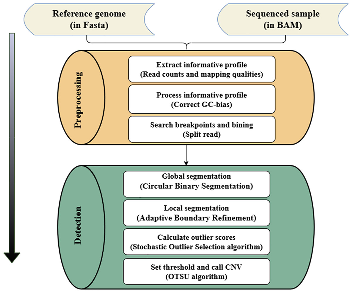
Figure 1: Workflow of SOSCNV.
The inputs include a reference genome (FASTA) and aligned sequencing data. The workflow consists of two major stages: preprocessing and detection. The preprocessing stage extracts sequencing signals, performs GC-content correction, and identifies breakpoints using split-read information. The detection stage applies a two-stage segmentation procedure (global and local segmentation) and uses SOS and OTSU algorithms to determine CNV regions.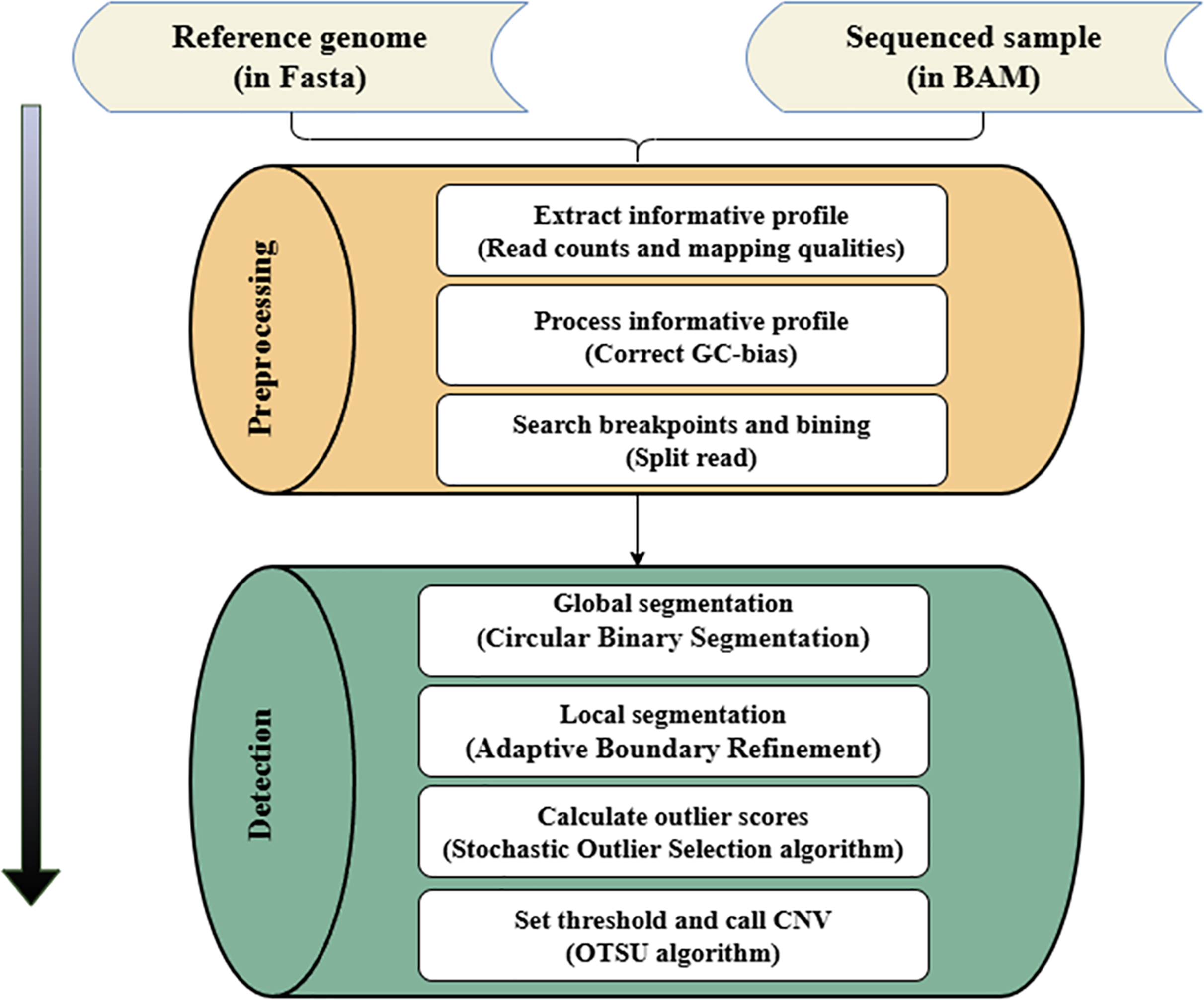
In the workflow diagram of the SOSCNV method, the alignment file in Binary Alignment Map (BAM) format and the reference genome file in Fasta format are regarded as input files (Li & Durbin, 2009). Among them, the BAM file can be generated by aligning sequencing samples (Bonfield & Mahoney, 2013) and the reference genome through the BWA-MEM algorithm, and then sorted by the SAMTools software (Li et al., 2009). In the preprocessing stage, the RD value is extracted as a feature signal, and according to the alignment information in SR strategy, the breakpoints of CNV regions in the genome sequence are determined. In addition to the RD signal, the mapping quality (MQ) of the reads in the window is also counted. MQ is employed to measure the quality of read alignments and to exclude low-quality bases, thereby reducing noise in the sequencing data. In the segmentation stage, a two-stage segmentation strategy is given. First, the circular binary segmentation (CBS) algorithm is used for global segmentation (Venkatraman & Olshen, 2007). Then, the large fragments obtained by the CBS algorithm segmentation are re-segmented into small sub-fragments, Then, the SOS algorithm models the feature signal and calculate the anomaly score. Finally, the OTSU algorithm determines the threshold and identifies the final CNV (Goh et al., 2018).
Preprocessing
In the preprocessing stage, it covers extracting alignment information, dividing the bins, correcting GC deviations and searching for breakpoints (Du et al., 2025a). The RD signal is regarded as the input feature of the model, which is the most important feature information in the RD-based detection strategy. After calculating the RD value at each position on the genome sequence, further processing is needed to meet subsequent detection requirements.
(1) Dividing windows and calculating RD and MQ signals
The reference genome is divided into consecutive, equal-sized, non-overlapping bins with a width of 1,000 bp. For each bin, the sequencing read depth information from the BAM file is calculated and marked as the initial RD. If a bin in the reference genome contains “N” bases, the initial RD of this bin is set to a negative value and the bin is marked as an abnormal bin; the RD value of such bins is excluded from further statistical analysis. For normal bins that do not contain “N” bases, the average read count across all bases within the bin is calculated as the RD value for that bin and is used in subsequent detection analysis, as shown in Formula (1). In this formula, represents the average read depth of the i-th bin, is the read count at the j-th position within the bin, and is the size of the i-th bin. This approach effectively reduces noise-induced fluctuations and lowers computational cost.
(1)
In addition to the RD signal, the MQ of the read segments within each bin is also calculated, as shown in Formula (2). In this formula, represents the average mapping quality of the i-th bin, denotes the mapping quality score at the j-th position within the bin, and is the size of the i-th bin. The MQ signal reflects the overall alignment reliability of reads in the bin, where higher MQ values indicate more confident alignments. By filtering out low-quality mapping positions and replacing unreliable base-level signals with the average MQ value, this approach effectively reduces the impact of noise on CNV detection results.
(2)
(2) GC correction
GC bias (Benjamini & Speed, 2012) is a key factor that causes the inconsistency between RD signal and sequence depth. In regions with low or high GC content, the RD value will deviate, which will affect the analysis of subsequent detection results. The GC content also has a certain correlation with the RD value. Specifically, it is manifested that the GC content in the CNV region may have a large difference compared with that in the normal region. Therefore, in the SOSCNV method, the GC content is also used as the input feature signal of the anomaly detection model. The following method can effectively correct the RD value of each window. as shown in Formula (3). Among Formula (3), and respectively represent the corrected RD value and the original RD value of the i-th bin, represents the average RD value of all bins, and represents the average RD value of all bins with the same GC content as this bin.
(3)
(3) Searching for possible breakpoints
SOSCNV employs a split-read strategy based on the CIGAR string to identify breakpoints. For alignment information in BAM files, it prioritizes read records that contain soft clipping or hard clipping operations. The presence of clipping indicates that part of the sequencing read could not be successfully aligned to the reference genome during the mapping process, and these unmapped segments may suggest potential CNV. Formula (4) summarizes the possible combinations of matching and clipping operations in the Compact Idiosyncratic Gapped Alignment Report (CIGAR) string. “M” denotes the continuous segment of the sequencing read that aligns to the reference genome, while “S” and “H” represent soft clipping and hard clipping in the CIGAR string, respectively. indicates that x bases are aligned to the reference genome; means that y bases remain unaligned but are kept in the read; and means that y bases are unaligned and removed from the read. When the clipped segment occurs before the aligned region ( and ), the breakpoint is assigned to the start position of the aligned block, i.e., . Conversely, when the clipped segment occurs after the aligned region ( and ), the breakpoint is assigned to the end position of the aligned block, i.e., .
(4)
Detection
Global segmentation and local segmentation
After the preprocessing is completed, the segmentation step will be executed, which includes two stages: global segmentation and local segmentation, with the aim of identifying consecutive regions with the same RD signal. Global segmentation is performed using the circular binary segmentation (CBS) algorithm. The CBS algorithm first searches for a continuous sequence of genomic windows. Based on the maximum statistic, the method compares the average RD value within a continuous window region to the average RD value of the remaining windows. If the difference between the two exceeds a predefined threshold, the position is considered a potential breakpoint. The region is then partitioned into new segments using this breakpoint as the boundary. This process is recursively repeated across the entire genome until no further significant change points can be detected, ultimately achieving multiple segmentations of the genome. Based on the divided segments, the RD value and GC content are recalculated, as shown in Formulas (5) and (6). Among formulas, and respectively represent the RD value and GC content in the i-th fragment, represents the size of the i-th fragment, and and respectively represent the RD value and GC content of each window contained in the fragment. After segmentation is completed, the total number of samples changes from the number of windows to the number of segments divided.
(5)
(6)
After the global segmentation is completed, proceed with local segmentation. Due to the substantial variation in the lengths of candidate segments produced by CBS segmentation, SOSCNV employs a local re-segmentation strategy to reduce the influence of length heterogeneity on subsequent analyses and to improve the local resolution of CNV detection. In this process, the candidate segments are further partitioned into uniformly sized sub-segments with fixed lengths. First, the length of the sub-segments needs to be defined. The size of sub-segment is related to the resolution of CNV detection. A smaller sub-segment can provide a higher breakpoint resolution, but it will lead to an increase in false positive events; while a larger sub-segment can improve the recognition accuracy, but it will cause additional false negative events. The length threshold of sub-segments is defined as . The parameter is flexible and can be selected based on the characteristics of the sequencing data. In practice, may be configured to 500, 1,000, 3,000 bp, or larger values to balance breakpoint resolution and noise robustness across different datasets. Subsequently, the segments with a length greater than are re-segmented into multiple consecutive sub-segments with a length of . If the length of the sub-segment does not reach , this fragment is merged into the previous sub-segment, and the segmentation continues on the concatenated segment. For sub-segments that do not require merging, their sequencing signals (RD and GC) are computed directly from the bins they cover. For sub-segments generated by merging a short residual fragment with the previous segment, the sequencing signals are obtained by averaging the RD and GC values of all bins contained in the merged interval.
Abnormal score calculation and confirmation threshold
After local segmentation is completed, the next step is to calculate the abnormal score. The purpose of this step is to quantify the degree of abnormality of each sub-segment, which helps in identifying potential CNVs more accurately. In anomaly detection algorithms, anomaly scores can be used to represent the degree of anomaly of each data sample. The anomaly score in the SOS algorithm is the probability value of anomalies between 0 and 1, so there is no need for additional normalization processing, avoiding the problem of large differences in anomaly score ranges on genomic data with different coverage levels. The outlier score represents the probability of a sample point being an outlier, and the higher the score, the greater the likelihood of it being an outlier. The SOSCNV algorithm primarily uses the preprocessed read depth signal and GC-content signal as the initial inputs. The abnormal score calculation process of the SOSCNV model can be seen as a transformation process of four matrices, and the specific steps are as follows:
-
(1)
Let denote the input segmentation matrix, where n is the number of segments, and the two columns represent the preprocessed RD and GC signals;
-
(2)
Calculate the dissimilarity matrix D based on the distance between each segmentation point;
-
(3)
Use the matrix D to calculate the correlation between segmentations and represent it with the matrix P;
-
(4)
Calculate the correlation probability matrix Q based on matrix P;
-
(5)
Calculate the anomaly score for each segmentation from the correlation probability matrix Q.
In Step 1, the input data sample set includes two features, namely the RD signal and GC content of each sub-segment, which are represented by a matrix M of size , where n denotes the number of sub-segments, as shown in Formula (7). Each row of the matrix M can be regarded as a sample point and is represented by a two-dimensional feature vector xi = [ , ].
(7)
In Step 2, the two features of the data points are used for the calculation of the dissimilarity between the data points. The dissimilarity is obtained through the Euclidean distance between two data points in the two-dimensional Euclidean space and is a non-negative scalar. The calculation process of the dissimilarity between the data points and is given by Formula (8).
(8)
It can be learned from the above formula that the dissimilarity matrix D is a symmetric matrix, that is, = . At the same time, the distance from a data point to itself is 0. The dissimilarity matrix D ( ) can be expressed in the form of Formula (9).
(9)
In Step 3, the similarity relationship between two data points is quantified through the degree of association. The higher the similarity between the two data points, the greater the degree of association. Conversely, the greater the dissimilarity, the smaller the degree of association. The calculation formula for the degree of association between the two data points is shown in Formula (10).
(10)
Here, represents the variance of the data point mi. In the SOS algorithm, each data point corresponds to a variance. The variance value is related to the density of the data point. Points with high density correspond to a smaller variance. The smaller the variance, the faster the attenuation of the degree of association; conversely, the larger the variance, the smaller the influence of dissimilarity on the degree of association. The SOS algorithm uses an adaptive method to determine the variance of each data point so that each data point has the same number of effective neighbors. The number of neighbors of a data point is called the complexity and is also the only parameter of the SOS algorithm. Each data point can have 1 to effective neighbors. By calculating the degree of association between data points, the association matrix P ( ) is obtained, as shown in Formula (11). The diagonal elements in matrix P are 0 because there is no association between a data point and itself. Different from the dissimilarity matrix D, matrix P is asymmetric. This is because the variance of each data point is generated through an adaptive method, and the probability that two data points have the same variance is extremely low, thereby causing the asymmetry of the association degree ( ).
(11)
In Step 4, the association probability matrix Q is obtained by normalizing the row vectors in the association matrix P. The calculation of the association probability value between two data points is shown in Formula (12).
(12)
Similar to matrix P, the correlation probability value between the data points themselves is 0. Based on the correlation probabilities between the data points, the anomaly score of each sample is calculated, as shown in Formula (13). Among Formula (13), represents the anomaly class, and the anomaly is a probability value ranging from 0 to 1. When the correlation probability value between a sample point and all other sample points is low, it is highly likely to be an abnormal point. Generally speaking, the segment represented by sample points with larger anomaly scores are potential CNV regions.
(13)
For different genomic data, the abnormal scores calculated by the SOSCNV model are also different. If a threshold of fixed size is used to classify the abnormal scores, it will produce certain deviations and cause inaccurate subsequent detection results. So, this article uses the OTSU to automatically obtain the thresholds applicable to various different genomic samples.
The OTSU algorithm is a global binary segmentation algorithm that dynamically obtains the threshold by traversing all the scores in the interval to maximize the variance between the normal class and the abnormal class. The abnormal score obtained by the SOS model is a probability value between 0 and 1. The abnormal score values of large abnormal samples are usually larger, and their number is much smaller than that of normal samples. Therefore, when using the OTSU algorithm to select the threshold, a range interval can be specified instead of starting from the minimum abnormal score to traverse until the threshold T that maximizes the variance between the normal class and the abnormal class is found. To improve computational efficiency, the OTSU algorithm can search for the threshold T that maximizes the between-class variance within a specified score interval (e.g., [0.5, 0.7]) where abnormal scores are more likely to fall. This avoids unnecessary traversal of very low or high scores while still adapting dynamically to the sample distribution. After T is determined, the abnormal score value of each fragment is compared with T, and the fragment with a score higher than T is determined as the CNV region. Then, the RD value corresponding to the CNV region is compared with the average RD value of the normal region to distinguish whether each variation region is copy number amplification or deletion.
Results and discussion
To verify the effectiveness of the SOSCNV method, comparative experiments were designed on both simulated data and real data. The performance of SOSCNV was compared with Manta, Matchclips2, RSICNV, and TARDIS in terms of precision, recall, and F1-score. Manta is a detection tool based on PEM and SR strategies, which constructs a breakpoint association graph and performs local assembly of candidate variants to efficiently detect diverse SVs and medium-sized indels in both germline and tumor samples. Matchclips2 is a detection tool based on the SR strategy, which detects breakpoints and identifies CNVs by analyzing soft clipping in CIGAR strings. RSICNV is a detection tool based on the RD strategy, which detects CNVs from high-coverage whole-genome sequencing data using a robust segment identification algorithm with negative binomial transformations. TARDIS is a variant detection tool based on RD, SR, and PEM strategies, which identifies candidate variant regions, clusters supporting evidence, and employs statistical modeling to accurately detect diverse SVs and CNVs from whole-genome sequencing data.
In the simulation experiments, short-read sequencing data were generated using SInC and Seqtk. SInC is a simulation toolkit designed for producing next-generation sequencing reads, allowing users to specify parameters such as read length, insert size, and sequencing depth. SInC models sequencing errors based on real data generated from Illumina instruments. However, GC bias inherent to Illumina sequencing can distort read-depth signals and affect variant analysis. To mitigate this effect, SOSCNV applies GC bias correction during the preprocessing stage. Seqtk was further employed to manipulate the reference genome sequences, in particular to adjust the proportion of copy number–altered regions, thereby controlling the tumor purity in the simulated data. In the simulation experiments, chromosomes 13 and 21 from GRCh38 were used as references to simulate four types of variations: tandem duplication, interspersed duplication, heterozygous deletion, and homozygous deletion. The simulated variation length ranged from 10 to 100kb on chromosome 13 and from 1 to 10kb on chromosome 21. Simulated datasets were generated under nine sequencing conditions by combining three sequencing depths (10×, 20×, 30×) with three tumor purities (0.4, 0.6, 0.8). To minimize random errors, 50 replicates were produced for each condition. In the comparative experiment on real data, three groups of sequencing samples from the 1,000 Genomes Project (https://www.internationalgenome.org/) and one real sequencing dataset from NCBI (https://www.ncbi.nlm.nih.gov/) were selected as analysis subjects. For these real samples, the variants annotated in the Database of Genomic Variants (DGV, https://dgv.tcag.ca/dgv/app/home; accessed February 2026) and Genome in a Bottle (GIAB, https://www.nist.gov/programs-projects/genome-bottle) were used as the ground truth for performance evaluation. Precision, recall, and F1-score are used as evaluation indicators. The definitions are as shown in the following formulas. In Formula (14), represents the number of True Positive events, which is the number of CNVs events correctly identified by the detection tools. When the variation region identified by the detection tools overlaps more than 50% with the real CNVs region, it is recognized as a true positive event (Du et al., 2025b). represents the number of False Positive events, which refers to the number of instances where normal regions are incorrectly identified as CNVs events. Precision is the ratio of the number of variation events correctly identified by the detection method to the total number of variation events detected. Formula (15) defines recall, represents the number of False Negative events, that is, the number of abnormal regions wrongly judged as normal events. represents the total number of CNVs events in the original sample. The F1-score is given by Formula (16) and is the average of precision and recall. The higher the F1-score, the better the performance of the detection algorithm.
(14)
(15)
(16)
Simulation experiment analysis
The results are shown in Figs. 2 and 3. The indicator values in the figure are the average values of the evaluation quantities in 50 samples for each configuration. The gray curve represents the F1-score. To ensure the fairness of the experiment, each method uses its default parameters.
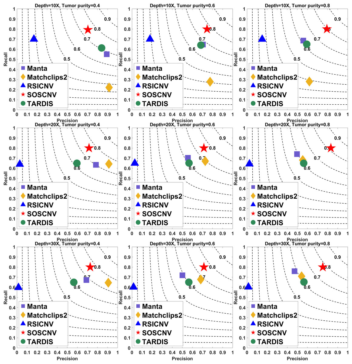
Figure 2: Performance comparison of five CNV detection tools on simulated data.
The simulated data are based on chromosome 13 and generated using SInC and Seqtk, including three sequencing depths, three tumor purities, and variant lengths of 10K–100K. Each subfigure represents a specific combination of sequencing depth and tumor purity. In each subfigure, the x-axis indicates precision, the y-axis indicates recall, and the position of each marker represents the F1-score of a tool under the corresponding experimental conditions.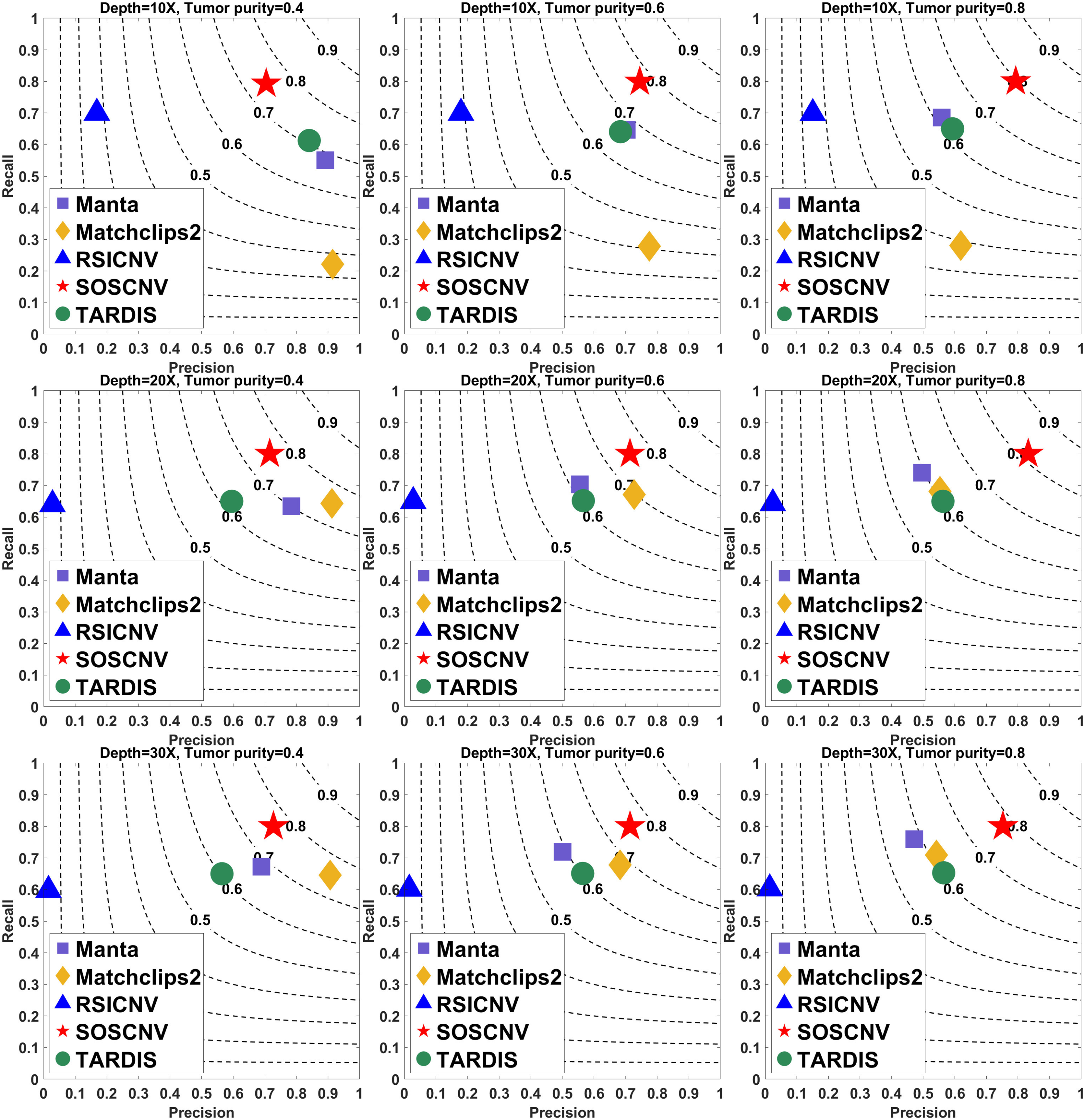
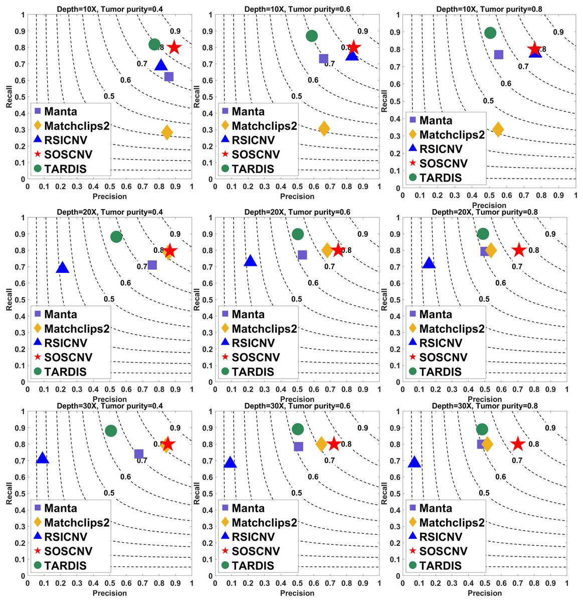
Figure 3: Performance comparison of five CNV detection tools on simulated data.
The simulated data are based on chromosome 21 and generated using SInC and Seqtk, including three sequencing depths, three tumor purities, and variant lengths of 1K–10K. Each subfigure represents a specific combination of sequencing depth and tumor purity.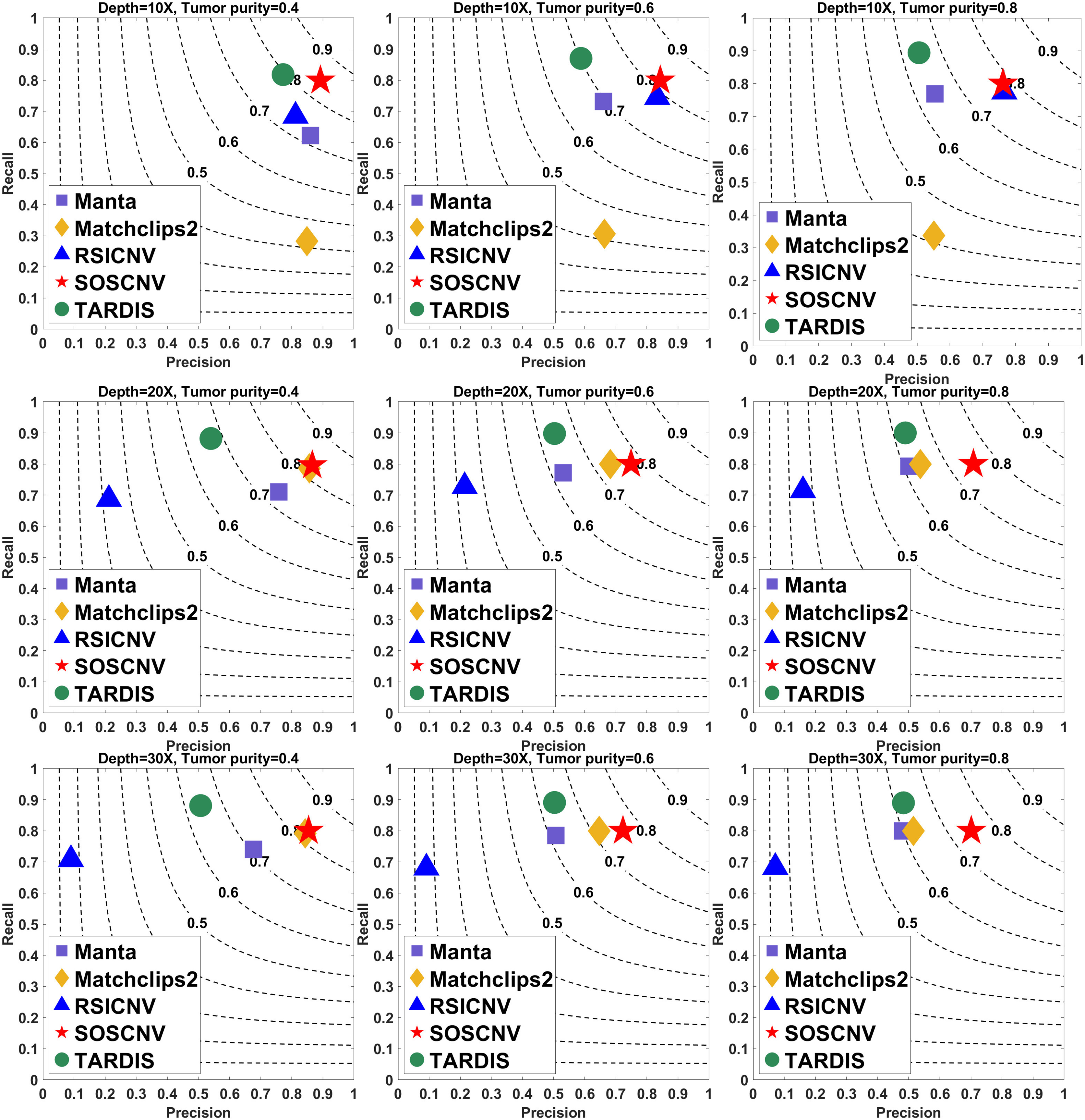
Regardless of whether the simulated data are from Chromosome 13 or Chromosome 21, the SOSCNV method consistently achieves the highest F1-scores across all combinations of sequencing depths and tumor purities, demonstrating superior overall detection performance. Overall, SOSCNV, Manta, and TARDIS exhibit strong robustness, as their detection performance is relatively unaffected by changes in sequencing depths, tumor purities, and CNV lengths. Specifically, on the simulated data from Chromosomes 13 and 21, Manta’s F1-scores consistently range between 0.6 and 0.7. For TARDIS, the F1-scores on Chromosome 13 also range from 0.6 to 0.7, whereas on Chromosome 21, they slightly increase to a range of 0.6–0.8 with greater fluctuation, suggesting that TARDIS performs more stably when detecting longer CNVs. In contrast, SOSCNV achieves F1-scores between 0.7 and 0.8 on Chromosome 13, and an even higher range of 0.75–0.85 on Chromosome 21, indicating better detection performance. Across both chromosomes, SOSCNV outperforms Manta and TARDIS. Meanwhile, RSICNV and Matchclips2 show opposite performance trends: RSICNV achieves higher F1-scores under low sequencing coverage than at higher depths, whereas Matchclips2 performs better at higher coverage levels, with noticeably lower F1-scores at 10 .
In the simulated data, Chromosome 13 is used to construct longer CNVs, whereas Chromosome 21 is used to construct shorter CNVs. SOSCNV consistently maintains high and stable F1-scores in both scenarios, achieving scores of 0.7–0.8 on Chromosome 13 and even higher scores of 0.75–0.85 on Chromosome 21. This indicates that SOSCNV is not only effective for long CNVs but also demonstrates enhanced sensitivity when detecting shorter CNVs, a scenario where many traditional methods typically struggle.
Moreover, the F1-scores of SOSCNV across different sequencing depths and tumor purities exhibit a narrower variance compared to other tools, suggesting that its performance is less affected by these common experimental variables. The method achieves a balanced trade-off between precision and recall, as reflected by its favorable positioning on the F1-score contour lines, without sacrificing one for the other. In contrast, other tools such as Manta and TARDIS tend to exhibit slightly lower F1-scores and greater fluctuations depending on CNV length and coverage, while RSICNV and Matchclips2 show more pronounced performance changes when sequencing depth varies.
Collectively, these observations highlight that SOSCNV offers not only superior average detection accuracy but also stronger robustness across different CNV lengths, sequencing coverages, and tumor purity conditions, making it particularly suitable for real-world applications where CNV size and sequencing quality can vary widely.
Real experimental analysis
To compare the detection performance of SOSCNV with several other tools on real data, samples from the Yoruba family trio in the 1,000 Genomes Project were selected, including NA19238 (mother), NA19239 (father), and NA19240 (daughter). In addition, the HG002 sample was downloaded from NCBI as another real dataset for evaluation. SOSCNV and four other tools were evaluated based on these four real samples. For performance assessment, the Database of Genomic Variants (DGV, https://dgv.tcag.ca/dgv/app/home) and Genome in a Bottle (GIAB, https://www.nist.gov/programs-projects/genome-bottle) were used as ground truth references. In the evaluation, the ground truth was derived from the GRCh38 reference genome, using the version released on February 25, 2020 (https://dgv.tcag.ca/dgv/app/downloads?ref=GRCh37/hg19; accessed February 2026). For the ground truth of the real data HG002, we used the GIAB benchmark released in November 2024 (https://ftp-trace.ncbi.nlm.nih.gov/ReferenceSamples/giab/release/AshkenazimTrio/HG002_NA24385_son/mosaic_v1.00/GRCh38/SNV/).
Figure 4 illustrates the performance of five CNV detection tools across four real human samples. The three bar plots respectively show the average precision, recall, and F1-score over the 22 chromosomes. As shown in the figure, SOSCNV achieves substantially higher precision in the NA19238 and NA19240 samples compared to other tools, indicating superior detection accuracy. Although Manta exhibits relatively high precision in the NA19240 sample, the number of detected CNVs is too small, resulting in a very low recall and thus lowering its overall F1-score. Due to the low sequencing depth of the three real samples, Mathclips2 is almost unable to effectively detect copy number variations. In the real data sample HG002, SOSCNV not only achieved the highest precision but also the highest F1-score, further demonstrating its robustness across different datasets. Overall, SOSCNV achieves the highest F1-scores across all four real samples, demonstrating that it outperforms the other four tools not only in simulated datasets with varying CNV lengths, sequencing depths, and tumor purities, but also in real-world data. Due to the large number of variants included in the DGV ground truth, although some detection tools achieve relatively high precision on certain variants, the number of true positives detected is still small compared with the total number of ground truth variants. Consequently, the recall of all five tools remains relatively low.
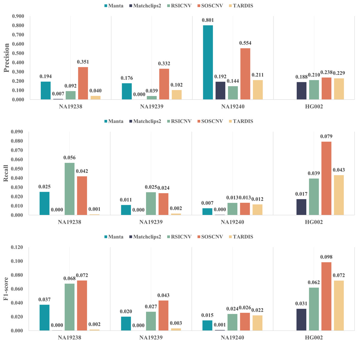
Figure 4: Detection performance of five CNV detection tools on real data.
The first subfigure shows the precision of each tool across four real samples, the second subfigure shows the recall, and the third subfigure shows the F1-score.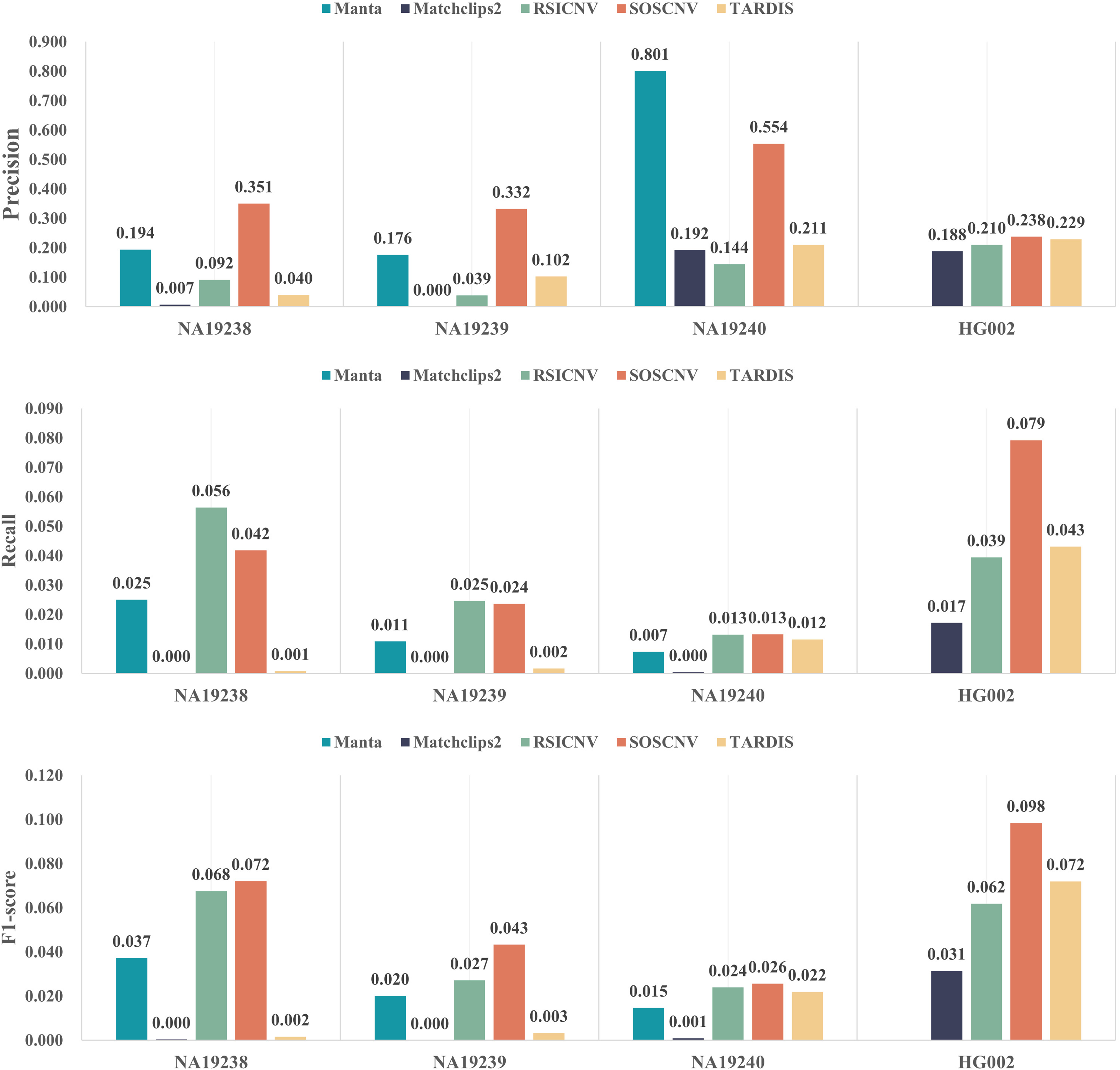
NA19238, NA19239, and NA19240 belong to the same family, making the Mendelian inconsistency rate a reliable metric for CNV evaluation. If a CNV detected in the offspring overlaps (50% reciprocal overlap) with a CNV of the same type in either parent, then the CNV is defined as the Mendelian consistent CNV, else the CNV is defined as the Mendelian inconsistent CNV. The rate of Mendelian inconsistent CNVs in the offspring is defined as Mendelian inconsistency rate (Liu, Wu & Wang, 2021). Table 1 shows the Mendelian inconsistency rates of the five CNV detection tools on the real data samples. RSICNV exhibited the lowest Mendelian inconsistency rate among all tools, which may be related to the larger number of CNVs detected by RSICNV: it identified the highest number of CNVs in NA19238, NA19239, and NA19240. In contrast, Manta, Matchclips2, and TARDIS showed relatively high Mendelian inconsistency rates, all exceeding 30%, while SOSCNV’s inconsistency rate was lower than that of these three tools.
| Detection tools | Number of CNVs detected in parents | Number of Mendelian inconsistent CNV | Mendelian inconsistency rate |
|---|---|---|---|
| Manta | 830 | 230 | 32.046% |
| Matchclips2 | 110 | 36 | 35.531% |
| RSICNV | 4,130 | 556 | 11.084% |
| SOSCNV | 903 | 202 | 21.906% |
| TARDIS | 548 | 92 | 33.236% |
Evaluation of detection time
Figure 5 compares the runtime of the five CNV detection tools across the three real data samples. All five detection tools were executed on the same computer, which was running Ubuntu 22.04.5 LTS, equipped with 16.0 GiB of RAM and a 13th Gen Intel® Core™ i7-13700F processor with 24 cores. As shown in the figure, Manta requires the longest runtime, whereas Matchclips2 is the fastest among the five tools. SOSCNV’s runtime is the second longest, just below Manta. The overall runtime of SOSCNV includes both the preprocessing and detection stages. While it is slightly longer than some other tools, this also represents an area for future improvement. Further optimization of runtime, particularly for large-scale datasets, would enhance its applicability in research and clinical settings.
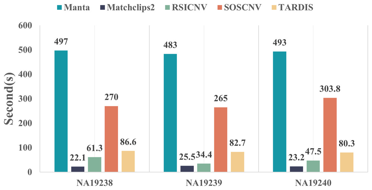
Figure 5: Comparison of runtime for five detection tools on real data.
Manta required the longest time to process the real data, while SOSCNV was slightly faster than Manta. Optimizing runtime to improve detection efficiency will be a key focus of future work for SOSCNV.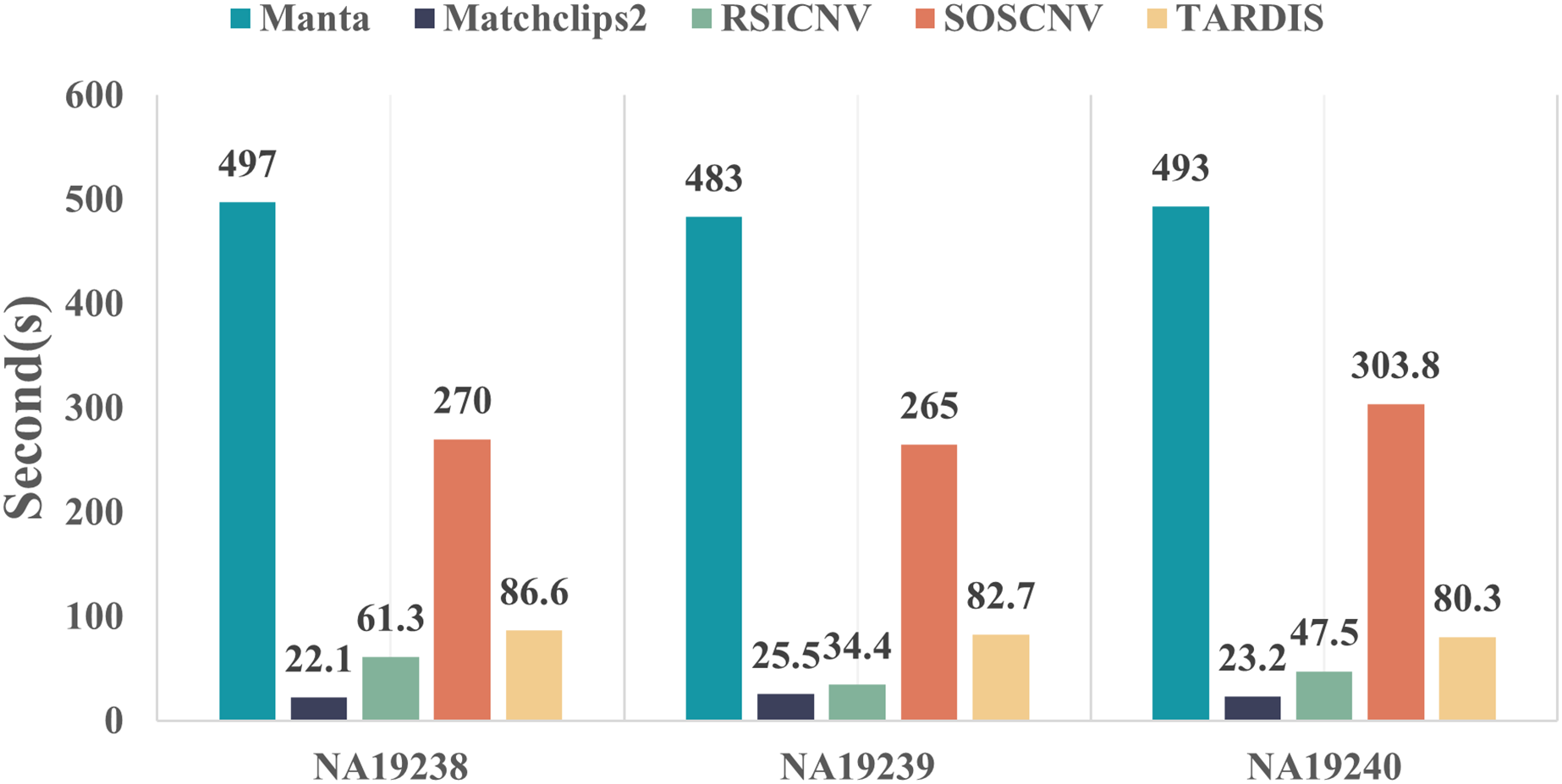
Discussion
We propose a method called SOSCNV to address the challenge of inaccurate breakpoint detection and low detection accuracy under complex sequencing conditions. SOSCNV employs a hybrid detection strategy that combines RD signals with SR signals to improve CNV detection accuracy. The RD signal is used to identify candidate CNV regions, while the SR signal is leveraged to accurately locate the breakpoints (Kosugi et al., 2019). By adopting a global-first and local-second segmentation strategy combined with the SOSCNV algorithm, the detection model first locates abnormal regions based on the correlation probability between segments. CNV regions are further determined by calculating adaptive thresholds. This approach improves breakpoint resolution and enhances the ability to detect low copy number events of complex sizes (Zhang, Liu & Duan, 2024). This article compares the SOSCNV algorithm with four other algorithms in terms of recall, precision, F1-score through the testing of 900 simulated data sets and four real data sets. The results show that the SOSCNV algorithm is superior to other algorithms in the ability to identify CNVs and significantly improves the precision, recall, F1-score, and overlap density score of CNV detection, demonstrating the effectiveness of the SOSCNV algorithm in detecting CNV.
Compared with the increasingly popular deep learning–based approaches in recent years, SOSCNV also possesses its own unique advantages. As an unsupervised detection model, SOSCNV does not require training or labeled data and can achieve high accuracy even under low sequencing coverage. In addition, its model structure is more intuitive, making it easier to interpret than deep learning–based methods. Of course, SOSCNV also has certain limitations. First, the tool was originally designed for second-generation sequencing data, and therefore its applicability to long-read sequencing is limited. Second, when processing data with high sequencing depth, the running time of SOSCNV increases substantially, resulting in higher computational costs. Therefore, future research could consider incorporating deep learning methods to enhance the suitability and efficiency of CNV detection in long-read sequencing data.