
Enhanced swarm optimization for feature selection in electroencephalogram classification: investigating visibility graph and persistent homology-based features
- Published
- Accepted
- Received
- Academic Editor
- Bilal Alatas
- Subject Areas
- Artificial Intelligence, Data Mining and Machine Learning, Optimization Theory and Computation
- Keywords
- EEG, Persistent homology, Visibility graph, Binary particle swarm optimization, Feature engineering, Classification
- Copyright
- © 2026 Ling et al.
- Licence
- This is an open access article distributed under the terms of the Creative Commons Attribution License, which permits unrestricted use, distribution, reproduction and adaptation in any medium and for any purpose provided that it is properly attributed. For attribution, the original author(s), title, publication source (PeerJ Computer Science) and either DOI or URL of the article must be cited.
- Cite this article
- 2026. Enhanced swarm optimization for feature selection in electroencephalogram classification: investigating visibility graph and persistent homology-based features. PeerJ Computer Science 12:e3617 https://doi.org/10.7717/peerj-cs.3617
Abstract
The analysis of high-dimensional, nonlinear electroencephalogram (EEG) remains challenging, particularly for non-medical EEG, which shows only subtle distinctions between data classes, compared to medical EEG. This study proposed a novel persistent homology (PH) pipeline by incorporating visibility graphs and an enhanced binary particle swarm optimization (BPSO) with four improvement strategies into a range of PH representations and filtrations, to classify non-medical EEG recordings in a visual recognition task under varying auditory conditions. By integrating multi-domain features and robust feature selection, the proposed pipeline fills a crucial gap left by earlier PH-based EEG studies that mainly focus on narrow, single-domain feature sets. The highest increases of 23.71% in accuracy and 17.77% in F1-score were achieved when classifying the alpha EEG from the O2 channel using k-nearest neighbors classifier. The comparative analysis demonstrated the superiority of the enhanced BPSO over standard BPSO, while persistence landscape, silhouette, Vietoris-Rips filtration, and weighted visibility graph consistently surpassed the others in performance. Alpha EEG exhibited better classification performance than beta EEG, indicating a stronger link between alpha activity and attentional modulation. The statistical significance test, hyperparameter sensitivity analysis, and benchmarking results using a public epilepsy EEG dataset validated the applicability of the proposed pipeline in different EEG analysis tasks. These findings corroborated the capability and impact of the proposed pipeline in complex EEG analysis, promoting the development of the brain-computer interfaces.
Introduction
With the advancement of data analysis techniques and technologies, there has been a surge in the study of electroencephalogram (EEG) in various domains. A significant portion of the existing literature is dedicated to the analysis of medical EEG data for detecting neurological diseases, such as epilepsy (Shah et al., 2024) and schizophrenia (Poetto & Duch, 2024), just to name a few. These clinical diagnostic studies typically emphasize statistically significant differences between EEG recorded from patients and control groups, and often focus on signals with dramatically increased amplitude or oscillation linked to symptom onset. In contrast, EEG recorded during non-medical applications, for instance in short cognitive tasks, generally has only subtle differences, making it challenging to identify stimulus-specific responses (Gupta, Beuria & Behera, 2024), or capture the implicit correlations between EEG and the underlying cognitive process (Li et al., 2022). Regardless of the difficulty, non-medical EEG analysis is crucial due to its broad potential for real-world applications, such as the development of smart systems, brain-computer interfaces (BCIs), and user-monitoring devices.
Although EEG is a portable technique that records brain activity signals with high temporal resolution, analyzing EEG signals remains challenging due to their low signal-to-noise ratios, non-stationarity, and inherent multivariate nature (Klepl, Wu & He, 2024). Besides, the naturally intricate and chaotic brain dynamics, even in healthy subjects, contribute to highly complex and nonlinear EEG signals (Rodriguez-Bermudez & Garcia-Laencina, 2015). Conventional EEG analysis methods, either time or frequency domain analysis, provide only a limited view of these complex interactions and nondeterministic processes (Sharma & Meena, 2024). While significant enhancements can be achieved with deep learning models such as classifying motor-imagery (Wang, Yao & Wang, 2025) and finger movements’ EEG signals (Wang & Wang, 2025) in non-medical applications, its challenges include the necessity for extensive training data and the potential for overfitting.
Topological data analysis (TDA), an approach from algebraic topology, has attracted growing interest in recent studies to address the challenges of EEG analysis (see the dedicated reviews (Xu, Drougard & Roy, 2021; Ling, Phang & Liew, 2025). Unlike traditional techniques, TDA excels in handling high-dimensional data, uncovering higher-order structures, and maintaining robustness against noise (Poetto & Duch, 2024). Persistent homology (PH) stands out as the predominant TDA tool for its ability to trace topological changes through filtration and extract stable, invariant features (such as connected components or loops, either in time series or point clouds) from brain network structures by transferring them into simplicial complexes. These topological features are originally summarized in the form of persistence diagram (PD) or barcode, but over time, other PH representations and vectorization methods have also been developed for use with machine learning models. Also, several filtrations exist in PH for data modelling.
However, PH may be more effective in applications where the key differences between data classes are revealed through extreme signal values, such as clinical diagnosis with medical EEG data (Turkeš et al., 2025), rather than the subtle changes in EEG that occur in response to cognitive stimuli (Gupta, Beuria & Behera, 2024) or other non-medical applications. Also, TDA may suffer from heterogeneous subject biases (Caputi, Pidnebesna & Hlinka, 2021). Although different PH representations allow for capturing the unique aspects of each PD or barcode, the multiplicity of available representations presents challenges for researchers since there is no single standard approach to guide the selection for harnessing the power of TDA in analyzing a particular EEG dataset.
Hence, this study’s primary goal is to leverage the large number of topological features extracted from different PH representations to capture richer non-medical EEG signal information. Consequently, feature selection becomes crucial for identifying the most significant features and eliminating redundancy, which helps reduce the risk of overfitting and enhances EEG classification (Al-Nafjan, 2022). A feature selection method, namely the particle swarm optimization (PSO), has been widely employed in EEG studies due to its simplicity, robustness, and computational efficiency (Sun et al., 2022). Recent works have introduced several PSO variants to enhance its effectiveness, such as quantum PSO with fewer parameters (Chen et al., 2023), the integration of Chebyshev distance for feature filtration ahead of particle search (Hashim Albohayah et al., 2025), and an evolutionary mutation strategy to replace PSO velocity update (Solano-Rojas, Villalón-Fonseca & Batres, 2023). However, these variants remain prone to local optima and parameter sensitivity, and none address multimodal features. Thus, we proposed several improvements to the standard PSO algorithm for use in our PH-based EEG classification.
Topological features alone may not fully capture the richness of information in the data (Kang et al., 2024). Combining features from different domains generally improves classification performance (Wang et al., 2023). Recently, complex network approaches, such as ordinal partition networks, recurrence networks, and visibility graphs (VGs), have gained significant attention for their ability to reveal the brain’s topological organization and information flow (Yao et al., 2024). Due to its interpretability and adaptability to both large and limited datasets (Sun & Xu, 2024), several VG variants, such as the horizontal and limited penetrable VG, have been adopted to identify schizophrenia and epileptic EEG (Belhadi et al., 2025; Niu et al., 2025). Building upon existing VGs, this study explores their applicability to non-medical EEG data.
Specifically, this study employed a range of PH representations and filtrations, as well as various VG methods to extract features from our non-medical EEG data of 45 subjects recorded during a visual recognition task under quiet, low, and high distraction conditions that mimic real-world environments. Precisely distinguishing such signals under different auditory conditions facilitates the development of advanced BCIs. Previous studies on PH-based EEG signal analysis have mainly focused on a narrow, single-domain feature sets, which restrict their applicability to offer more generalizable insights into EEG data. This study addresses this gap by examining a wide range of methods and proposing a novel signal analysis pipeline that integrates TDA, complex network, and swarm optimization techniques. In terms of dataset analysis, this study conducts an extensive examination of multiple EEG frequency bands and sliding window approach for providing improved robustness in classifying non-medical EEG. The proposed pipeline was comprehensively evaluated using statistical significance testing, hyperparameter sensitivity analysis and benchmarking with a publicly available epilepsy EEG dataset.
Our findings indicate that two PH representations (namely, persistence landscape and silhouette), Vietoris-Rips filtration, and weighted VG features, exhibit superior performance. The alpha EEG from O2 channel with k-nearest neighbor classifier achieved accuracy and F1-score increments of 23.71% and 17.77% respectively, outperformed beta EEG. Furthermore, statistical tests confirmed that these gains in our enhanced binary PSO are statistically significant. These results demonstrate the proposed pipeline’s robustness and its ability to improve the classification accuracy across different classifiers.
Materials and methods
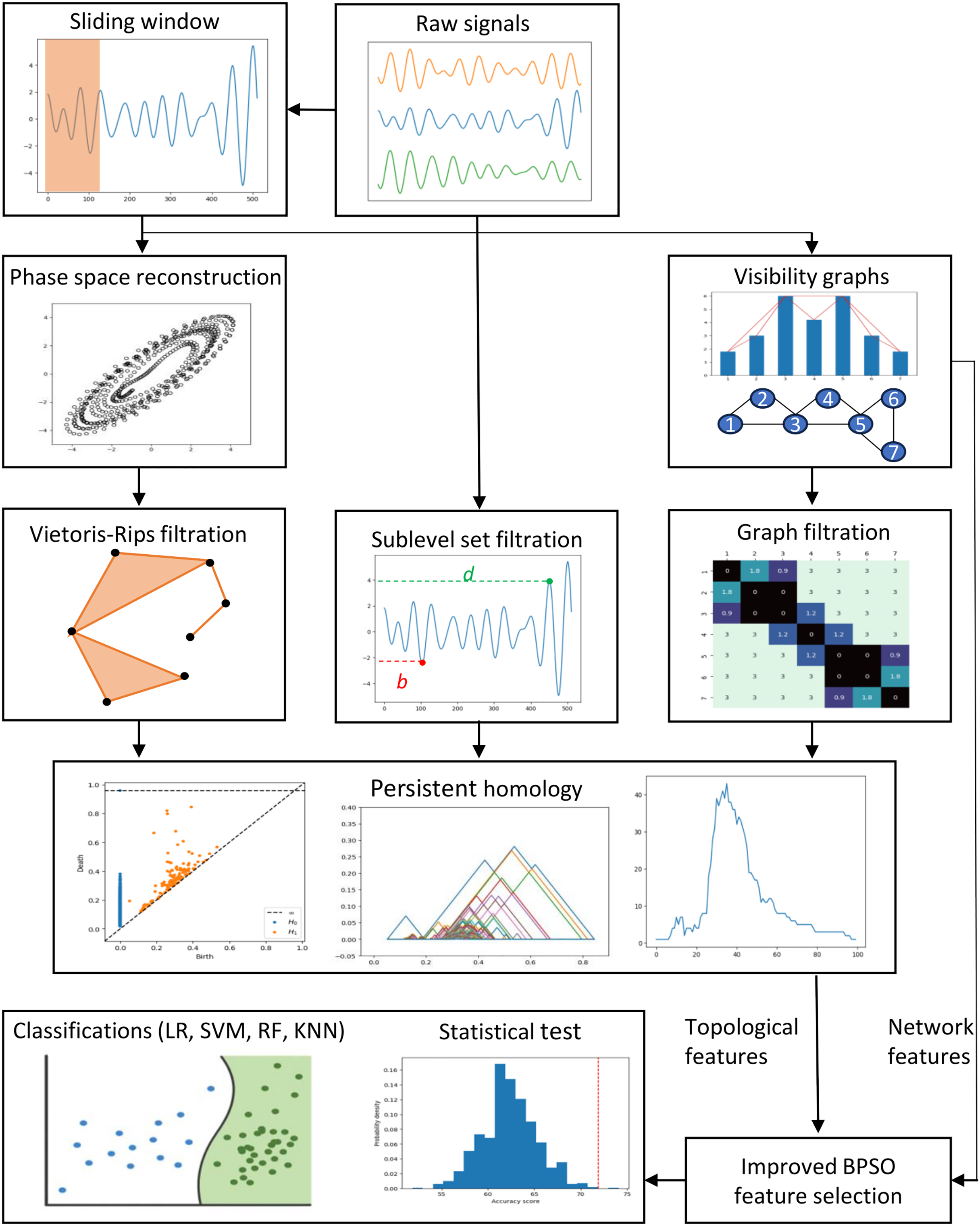
This section describes the data, preprocessing, feature engineering, and classification methods. Figure 1 depicts the study’s methodology flow. We first discuss the preprocessing approaches, including the sliding window, phase space reconstruction, and VG methods. Then, we focus on the EEG feature extraction using VGs and PH representations constructed through different PH filtrations. We then highlight the enhanced binary PSO feature selection method proposed in this study. Lastly, we emphasize the experiment settings, evaluation metrics, statistical tests, and the supervised machine-learning classification models applied to classify our EEG data.
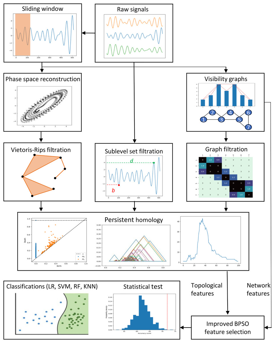
Figure 1: Proposed methodologies and EEG classification flow in this study.
Data source and preprocessing
This study analyzed both non-medical and medical datasets. The primary focus of this study is the non-medical EEG data collected in the previously published work by Liew et al. (2023), which includes recordings from a group of 45 subjects (25 males and 20 females selected based on predefined requirements, such as gender, health, age, and vision). A total of 15 participants were recruited for each of the three age groups (i.e., 18–25, 26–35, and 36+ years). All the subjects had a normal vision or corrected normal vision. Participants identified an image, focused on subsequent visual stimuli, and responded by clicking the mouse when the target image appeared. The experiment consisted of 150 trials, during which the target image was shown 60 times. During data collection, electrodes were placed according to the International 10–20 system, with the right earlobe as the reference and the right wrist as the ground. The sampling rate was 512 Hz, and no filtering was applied to avoid information loss. EEG signals were recorded under three simulated conditions: (a) quiet, (b) low distraction, and (c) high distraction, designed to mimic different real-world environments. An audio clip of regular office noise (≈55 dB) was played to simulate a low-distraction condition, while irregular office sounds (printer, stamping, phone ringing, etc.) were played at a sound level of 70 dB to simulate high-distraction condition. These sound levels were chosen to prevent auditory injury.
After recording, filtering, segmentation, and artifact rejection were performed to eliminate unwanted signals. A finite impulse response bandpass filter with cut-off frequencies of 8–13 Hz and 13–30 Hz was applied to extract alpha and beta bands. The signals were then segmented by trial, and any trials with amplitudes exceeding 100 μV—indicative of body movements or other artifacts—were excluded. Normal EEG amplitudes typically range from 0.5 to 100 μV (Teplan, 2002). While the dataset contains recordings from 21 electrodes, this study focused on five—T5, T6, O1, O2, and OZ—due to their relevance in auditory and visual processing.
Larger datasets generally enhance classification performance, while smaller ones risk overfitting (Althnian et al., 2021). A sliding window technique increases data volume and improves accuracy effectively (Zhao & Liu, 2023). In this study, we applied a non-overlapping sliding window of 250 Hz in one of our experiments to divide the original EEG time series with 512 data points into two segments, discarding the last 12 data points. This technique doubles the sample size for our classification and aids in capturing the transient patterns or anomalies that might be diluted in the entire signal. We presented all the non-medical EEG analysis results in Experiments I to V.
For the medical dataset, a publicly available epilepsy EEG dataset (namely the Bonn dataset) was used to benchmark the proposed methodology. Collected by the Department of Epileptology at the University of Bonn, Germany (Andrzejak et al., 2001), this dataset consists of five subsets labeled as Z, O, N, F, and S. Each subset contains 100 segments of single-channel EEG recordings. Each segment represents a time series signal with a length of 23.6 s (4,097 data points) sampled at 173.61 Hz. Subsets Z and O comprise the EEG recordings from five healthy awake individuals with their eyes open (Z) and closed (O), respectively. Meanwhile, subsets N, F, and S include the EEG signals recorded from five epilepsy patients. EEG signals were measured during seizure-free intervals in subsets N and F, while subset S contains signals measured during seizures. We focused on classifying EEG data from subset S against other subsets, excluding subset O, as in other relevant studies. We standardized the dataset before feature extraction and trimmed each segment to 5.9 s, a segment size used by Zhen, Yue & Liu (2024), to reduce the computational time while ensuring high EEG classification performance. We compared our findings with those of similar classification studies in Comparative Analysis section.
Ethics approval and consent to participate
For the non-medical EEG data collected in the previously published work by Liew et al. (2023), the ethical approval had been obtained from the Medical Research and Ethics Committee from Ministry of Health Malaysia. All data collection performed in Liew et al. (2023) were in accordance with guidelines registered in NMRR-14-1180-21356. Written informed consent was obtained from all participants after a full explanation of the study objectives and procedures.
Phase space reconstruction
Phase space reconstruction (PSR) captures complex brain dynamics, aiding in the extraction of distinguishing EEG features (Kaur et al., 2020). PSR transforms one-dimensional time series into a higher-dimensional data cloud using time delay embedding. Time delay embedding includes two key parameters: the time delay (τ) and the embedding dimension (m). The selection of the optimal values of these parameters has been well-studied, and various strategies have been proposed (Tan et al., 2023). In this study, we determined the optimal τ and m for each EEG time series using the average mutual information and false nearest neighbor methods. We then utilized the embedded EEG data to construct the PDs for feature extraction.
Visibility graph
A visibility graph is a time series analysis technique that converts time series data into a scale-free graph, capturing long-term temporal dependencies and chaotic time series properties (Bhandari et al., 2024). In a visibility graph, each time series point corresponds to a node, with edges forming between nodes that meet the visibility criteria. Specifically, two nodes, at and at , are connected if all intermediate nodes satisfy the condition in Eq. (1).
(1)
Different VGs have specific features and applications. In this study, we employed the natural and horizontal VGs with variations (weighted and limited penetrable) to convert our EEG time series into a complex network and extract significant network features for classification.
Natural and weighted visibility graph
A natural visibility graph (NVG) is constructed by mapping consecutive time series points onto the time axis, representing each value as a vertical bar (Azizi & Sulaimany, 2024). An edge is formed between two points whenever the heads of their vertical bars are visible from each other despite the presence of the intermediate bar.
While the NVG is an undirected and unweighted graph, the weighted visibility graph (WVG) extends it by assigning weights to edges based on the degree of visibility between time series points. WVG is often applied to discriminate various EEG signal types, such as detecting epileptic EEG (Supriya et al., 2016). In constructing WVG, different values, such as the Euclidean and horizontal distance, can be assigned as the edge weight. In this study, we used the absolute slope, as defined in Eq. (2), as our edge weight.
(2)
Figure 2 illustrates the NVG and WVG for a small synthetic EEG signal. For NVG in Fig. 2A, all the edges are assigned the same value regardless of their absolute slope value. In contrast, the larger the slope between two bars, the bigger the weight of the edge between them in the WVG, as shown in Fig. 2B.
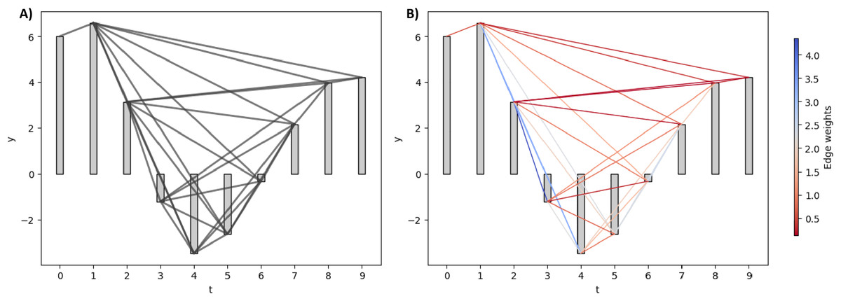
Figure 2: Natural and weighted visibility graph of a small synthetic EEG signal.
(A) NVG of the synthetic signal. (B) WVG of the synthetic signal. The edges are colored based on their weight values.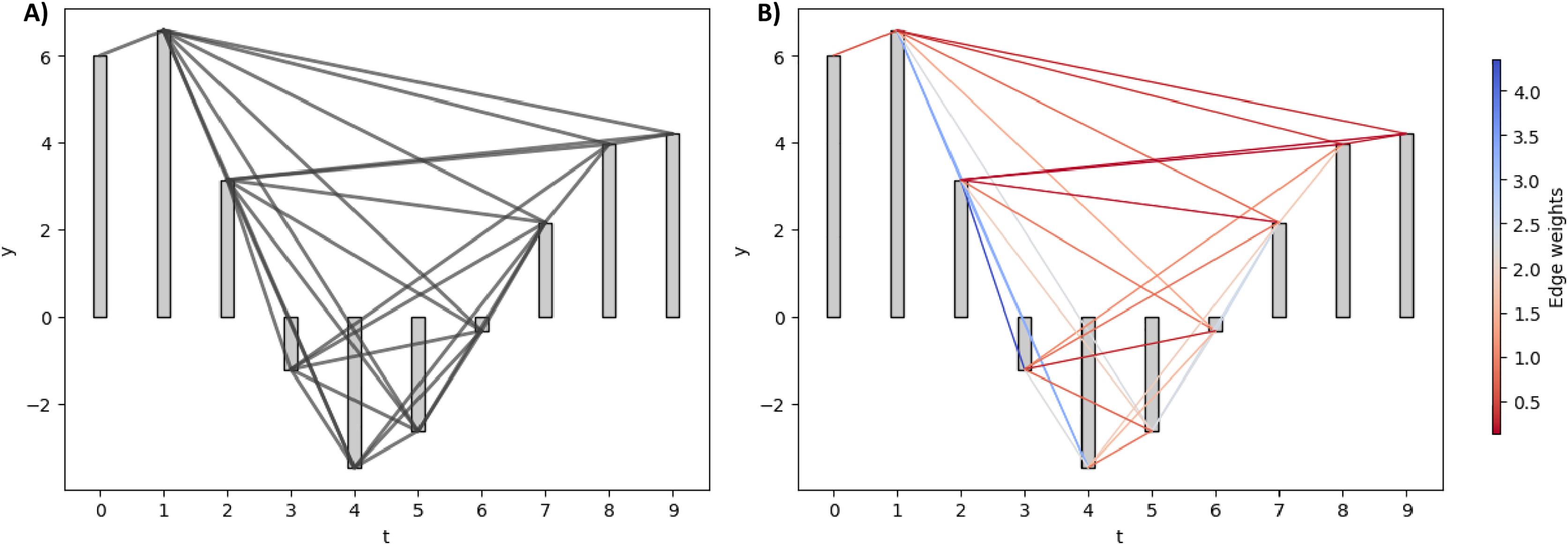
Horizontal and limited penetrable visibility graph
Real-world VGs can be extremely large, making them computationally complex and impractical to analyze. To address this, Luque et al. (2009) introduced the horizontal visibility graph (HVG), which reduces connections while preserving the temporal structure. Unlike NVG, HVG connects nodes based solely on horizontal lines of sight. The visibility condition between two nodes and with the presence of a middle rod is defined in Eq. (3).
(3)
HVG can also be directed and weighted, but we sticked to undirected and unweighted HVG in this study for simplicity.
Rather than reducing graph edges, the limited penetrable visibility graph (LPVG), which increases connectivity compared to VG, was used in Wang et al. (2016). LPVG enhances the VG algorithm by mapping a time series onto a graph while preserving its temporal characteristics. Moreover, LPVG demonstrates greater noise tolerance than VG. Its connectivity criterion allows a specified number of obstacles to be ignored, as defined in Eq. (4).
(4)
The parameter l represents the permeability limit, permitting a fixed number of bar penetrations to reduce the impact of noise. Specifically, we applied the limited penetrable horizontal visibility graph (LPHVG) with a penetrable limit of two to extract network features from our EEG time series.
Figure 3 elucidates the HVG and LPHVG of the same synthetic signal as in Fig. 2. It is clear that the number of connections in HVG is fewer (Fig. 3A) compared to its corresponding VG (Fig. 2). Also, every bar in an LPHVG (Fig. 3B) has denser connectivity than its corresponding HVG (Fig. 3A). The pink lines in Fig. 3B are the additional connections between bars when we granted a permeability limit of two to the HVG in Fig. 3A.
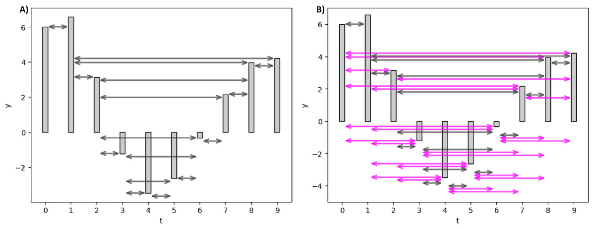
Figure 3: Horizontal and limited penetrable visibility graph of a small synthetic EEG signal.
(A) HVG of the synthetic signal. (B) LPHVG of the synthetic signal. The pink lines are the additional connections between corresponding bars with the permeability limit of two.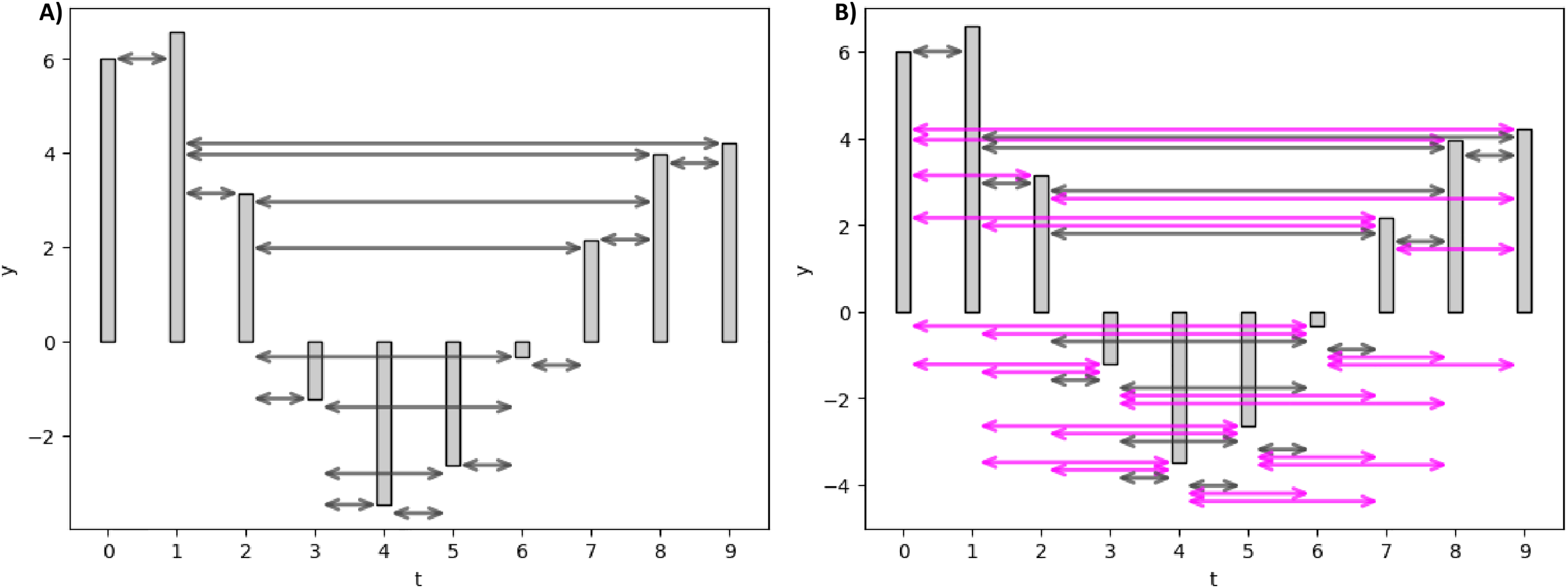
Feature extraction
After the preprocessing stage, we extracted complex network features from the constructed VGs. Then, we computed PH for our EEG using different filtrations that work with distinct EEG time series representations, including raw signals, point cloud, and VG. We extracted various topological features, including persistence statistics and other PH representations, from the resulting PDs.
Specifically, PH is a TDA method that captures structural changes in data across multiple spatial resolutions (Phang et al., 2024). PH computation involves representing the data cloud as simplicial complexes by applying filtration to track changes in geometric characteristics of the data and summarizing these changes with a persistence barcode or diagram. Different filtration methods analyze the geometric information of data in distinct ways. Hence, the following subsections elaborate on the critical steps involved in the PH-based approach, including types of filtrations, a brief description of the persistence statistics, and various PH representations.
Types of persistent homology filtrations
In this study, we investigated three types of filtrations: the Vietoris-Rips (VR), sublevel set, and graph filtration. In VR filtration, a distance parameter ε varies, forming an n-simplex when the pairwise distance between all points in the simplex is at most ε (Schweidtmann et al., 2022). At the early stage of the VR filtration, ε is very small, and only 0-simplexes (i.e., single points) exist. As ε increases, edges and filled triangles between data points emerge, creating 1- and 2-simplexes. Once the dataset is encoded as a nested VR complex, one tracks the birth and death of topological features within the simplexes (n-dimension homology classes, Hn) as the filtration progresses. In this study, we analyzed the lifespan of connected components (H0) and holes (H1), summarizing them in PD.
In sublevel set filtration, the evolution of the connected components in the raw EEG signal is tracked by focusing on their local critical points. Topological features extracted from our EEG time series through this filtration are limited to a single topological dimension (i.e., H0) rather than spanning multiple dimensions (for instance, H0 and H1 in VR filtration). Instead of a distance parameter used in VR filtration, sublevel set filtration employs a horizontal reference line that moves from the EEG signal’s minimum point to its maximum value as the threshold. As the threshold line ascends, we recorded the time whenever the line reaches the local minima and maxima of the signal, marking the birth and death of a connected component. Specifically, the most recent minimum point is paired with the following maximum point, leaving the oldest minimum point in the sublevel set for the pairing with a later maximum point (Wang, Ombao & Chung, 2018).
The last filtration we employed is the graph filtration presented in the study by Zhen, Yue & Liu (2024). While VR filtration is computed on the two-dimensional point cloud obtained from the phase space reconstruction of the EEG signal, and sublevel set filtration is on the raw EEG signal, graph filtration is carried out on continuous EEG time series transformed into complex networks. Hence, for graph filtration in this study, we first converted our continuous EEG data into discrete VG and computed its adjacency matrix. The adjacency matrix contains either a zero value or the weight of the edge between two data points (i and j). We then transformed the adjacency matrix into a distance matrix using Eq. (5).
(5)
The distance matrix measures the difference between each element and the maximum element in A. This transformation ensures that nodes with stronger connections appear closer. The resulting distance matrix becomes the input for generating PDs.
As a preliminary example to showcase the different traits of these three filtrations, we presented the PDs of the T5 signal recorded under quiet condition from Subject One in Fig. 4. The sublevel set filtration will typically yield PD with broader ranges of persistence values, possibly including negative values (see Fig. 4B), as it captures geometric information directly based on signal amplitude rather than pairwise distances between data points as in VR and graph filtrations. When examining the distance between the points and the diagonal line in the PDs, the PDs derived from VR and sublevel set filtrations show points with long lifespans. In contrast, the points in the PD constructed through graph filtration tend to have relatively shorter lifespans overall.
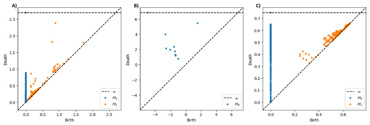
Figure 4: Persistence diagrams for T5 signal from subject one under quiet condition constructed using different PH filtrations.
(A) PDs constructed through Vietoris-Rips, (B) sublevel set, and (C) graph filtrations.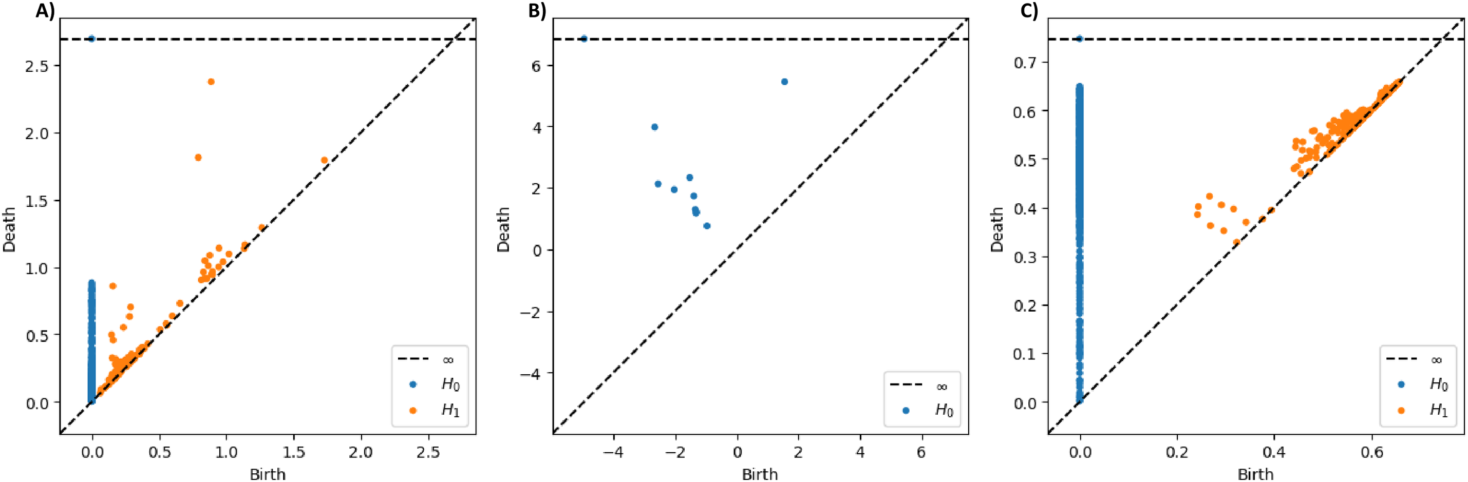
Persistence statistics
After constructing PDs from the EEG data, we extracted multiple persistence statistics features for the classification. We computed the maximum, sum, mean, median, standard deviation, range, interquartile range, and coefficient of covariance of the lifespan (l), birth (b), and death (d) time of H0 components and H1 holes in each PD. Notably, we excluded the statistics of H0 components’ birth as all H0 have a birth time of zero. The lifetime of the H0 and H1 is crucial as longer-persisting events often indicate meaningful structures, whereas shorter-lived ones are more likely to represent noise.
In addition to conventional statistical metrics, we recorded the total count of H0 and H1 in each PD. We also counted the number of relevant H0 and H1, defined as those that live at least half as long as the most persisting H0 and H1. Furthermore, we calculated the Wasserstein (W) and Bottleneck (B) distance between our PD (D) and an empty PD with diagonal only (D0) using the formulas in Eqs. (6) and (7).
(6)
(7)
These additional features are essential as they consider the overall structure of the PD rather than individual values, hence reducing the influence of outliers with extreme lifespans.
Persistent homology representations
While PDs encapsulate valuable information about the “shape” of a dataset, their direct application in machine learning and statistical contexts is challenging (Berry et al., 2020). Shape-based features from these diagrams may lack stability, as slight perturbations in the dataset can introduce or eliminate numerous points with short lifetimes (Karan & Kaygun, 2021). To address this, we transformed PDs into one- or two-dimensional functional summaries and vectorized representations, including persistence landscape, entropy, image, silhouette, and Betti curve, to extract additional features. Except for persistence entropy, most PH representations produce finite-dimensional value vectors. Therefore, we reduced them into single-value features through L1 and L2 normalization for the classification. Table 1 provides brief descriptions of each PH representation used in this study.
| PH representations | Description |
|---|---|
| Persistence landscape | A set of functions that represent different layers of the union of isosceles triangles generated through a piecewise linear function that summarizes the birth and death information of all points in a PD (Bubenik, 2015). |
| Persistence entropy | A real-valued measure that captures the variability in the lifespan of all points in a PD (Chintakunta et al., 2015). |
| Persistence image | A grid-based heatmap that highlights the presence and significance of high and low persistent features within the point cloud (Adams et al., 2017). |
| Persistence silhouette | A single weighted average function that consolidates all the layers of the landscape functions (Chazal et al., 2014). |
| Betti curve | A function that summarizes the Betti number (total number of Hn points in PD) over time (Umeda, 2017). |
Visibility graph based features
Based on the VGs generated from the EEG signal, we can directly extract network features for EEG classification, including the average (weighted) degree, average (weighted) shortest path length, modularity, density, transitivity, local and global efficiency, average clustering coefficient, and degree assortativity. Table 2 gives concise definitions and descriptions of each of these features.
| Network features | Definitions/Descriptions |
|---|---|
| Average (weighted) degree | The mean (edges weight) number of edges per node in the VG that measures the strength of connectivity between nodes (Poudel et al., 2024). |
| Average (weighted) shortest path length | The mean of the shortest paths (weight) between all pairs of nodes that measures the information flow in the network (Poudel et al., 2024). |
| Modularity | A measure of how effectively the nodes in the VG are grouped into communities. High modularity indicates that the VG has denser intra-community and sparser inter-community connections (Poudel et al., 2024). |
| Density | The actual number of edges divided by the maximum possible number of edges in a VG, highlighting the differences in the number of edges across VGs (Zhang et al., 2023). |
| Transitivity | Measures the likelihood that two connected nodes have a common neighbor, forming a closed triangle that shows interconnectivity (Azizi & Sulaimany, 2024). |
| Local efficiency | The average global efficiencies of subgraphs formed by each node’s direct neighbors, measuring how information is exchanged with these neighboring nodes (Azizi & Sulaimany, 2024). |
| Global efficiency | The average of the inverse shortest path lengths between all nodes, while a greater global efficiency reflects a network’s ability to transmit or integrate information more effectively (Zhang et al., 2023). |
| Average clustering coefficient | The average number of typical connections between a node and its neighbors that highlight the average tendency for these neighbors to form complete graphs (Zhang et al., 2023). |
| Degree assortativity | Measure of the tendency of a node to connect to other nodes with similar degrees (Lee et al., 2024). |
Category of features
As this study utilized 71 EEG features obtained from persistent homology and complex network approach, and within the persistent homological based features, numerous PH representations and persistence statistics were employed, we grouped the features into three broad categories, as listed in Table 3. It is restressed that the grouped features from f33 to f62 in persistence statistics category do not include the birth for H0 as all H0 have a birth time of zero.
| Category | Symbol | Features |
|---|---|---|
| PH representations | f1–f2 | L1 & L2 norms of the first H0 landscape layer |
| f3–f4 | L1 & L2 norms of the first H1 landscape layer | |
| f5–f6 | L1 & L2 norms of the H0 landscape layers average | |
| f7–f8 | L1 & L2 norms of the H1 landscape layers average | |
| f9–f10 | H0 and H1 normalized entropy | |
| f11–f12 | L1 & L2 norms of the H0 image | |
| f13–f14 | L1 & L2 norms of the H1 image | |
| f15–f16 | L1 & L2 norms of the H0 silhouette | |
| f17–f18 | L1 & L2 norms of the H1 silhouette | |
| f19–f20 | L1 & L2 norms of the H0 Betti curve | |
| f21–f22 | L1 & L2 norms of the H1 Betti curve | |
| Persistence statistics | f23 | Wasserstein distance |
| f24 | Bottleneck distance | |
| f25–f26 | Number of H0 and H1 points | |
| f27–f28 | Lifespan of the most persistent H0 and H1 point | |
| f29–f30 | Number of H0 and H1 points with lifespan at least half of the maximum lifespan | |
| f31–f32 | Sum of points’ lifespan for H0 and H1 | |
| f33–f37 | Mean of points’ lifespan, birth, and death for H0 and H1 | |
| f38–f42 | Median of points’ lifespan, birth, and death for H0 and H1 | |
| f43–f47 | Standard deviation of points’ lifespan, birth, and death for H0 and H1 | |
| f48–f52 | Interquartile range of points’ lifespan, birth, and death for H0 and H1 | |
| f53–f57 | Range of points’ lifespan, birth, and death for H0 and H1 | |
| f58–f62 | Coefficient of variance of points’ lifespan, birth, and death for H0 and H1 | |
| Weighted visibility graph | f63 | Average weighted degree |
| f64 | Average weighted shortest path length | |
| f65 | Modularity | |
| f66 | Density | |
| f67 | Transitivity | |
| f68 | Local efficiency | |
| f69 | Global efficiency | |
| f70 | Average clustering coefficient | |
| f71 | Degree assortativity |
Feature selection
After extracting 71 features from the EEG data, feature selection is necessary to identify the most relevant subset for classification. We applied binary particle swarm optimization (BPSO) algorithm to search for the optimal subset of features from the 71 available that yields the highest classification accuracy. Moreover, we introduced several strategies to address the standard BPSO limitations and enhance its efficiency.
Binary particle swarm optimization
PSO is a population-based algorithm for solving continuous and discrete optimization problems. Inspired by the collective behavior of birds and fish (Qiao et al., 2024), PSO enables individual particles to explore a solution space, adjusting their trajectories based on shared group knowledge to converge toward the global optimum. Each particle i is defined by two attributes: a velocity vector and a position vector , where j represents feature j in the solution space. The velocity vector dictates the movement direction, while the position vector corresponds to a candidate solution. The velocity and position updates follow the Eqs. (8) and (9).
(8)
(9)
In the equation, denotes the best position previously attained by particle i at iteration k, while Gbest represents the best position found by the entire swarm. We used 100 particles and set the maximum iteration to 200 in this study. The acceleration constants and regulate the balance between local exploitation and global exploration. Adjusting the values of and alters the influence of personal and global best on updating the particles’ velocities, facilitating the exploitation of particles around local best, or the exploration of particles in a broader area. The terms and are random values uniformly distributed in to enhance search randomness. The inertia weight parameter controls the search range of the swarm, helping balance global and local search tendencies. In standard PSO, is dynamic, as defined in Eq. (10), to optimize exploration and exploitation.
(10) where and represent the maximum and minimum inertia weight, while Mk denotes the maximum iterations. The , , , and are set to 2, 2, 0.9, and 0.4, respectively, in the standard PSO.
PSO was initially designed for continuous optimization, but Kennedy & Eberhart (1997) later introduced BPSO for discrete problems. Unlike standard PSO, where Pbest, Gbest, and position take continuous values, BPSO represents them as binary values (0 or 1) to indicate feature selection in a given solution. Besides, BPSO employs a sigmoid function to transform velocity and update particle positions, as defined in Eq. (11).
(11) where rand is a random number within the range of .
PSO is widely used in optimization due to its simplicity, fast convergence, effectiveness, and strong generalization (Xie et al., 2021). However, it has notable limitations, including susceptibility to local optima and inefficient fine-tuning. Since PSO relies solely on the global best solution for coevolution, particles do not exchange information and lack diversity. Moreover, the algorithm often revisits previously explored regions, as particles strictly follow their historical best experiences, leading to premature convergence and early stagnation (Shaqarin & Noack, 2023).
To address these limitations, researchers have developed various enhanced PSO algorithms for different applications. Common improvements involve adjusting parameter distributions, modifying position update strategies, optimizing swarm initialization, and integrating other intelligent algorithms (Qiao et al., 2024; Zhao et al., 2024). However, many PSO variants incorporate complex improvement strategies yet still struggle with local optimum traps and slow convergence (Emambocus et al., 2021). Hence, we proposed relatively simple approaches that enhance the BPSO feature selection performance, especially with feature input from numerous categories.
Improvement strategy 1: swarm division based on feature categories
The first step of BPSO implementation is initiating a population. In this step, we divided our population into multiple sub-swarms based on our extracted feature categories, as in Table 3. We separated our 100 particles into five groups of 20 particles. The first three groups search for the optimal solution in the solution spaces where a particular feature category is excluded (i.e., groups 1, 2, and 3 search within spaces that have no graph, persistence statistics, and PH representations features, respectively). Furthermore, the fourth group explores the area with all features but not H0 topological features to investigate the discriminative power of 0-dimensional homology. The last group is free to select any features as the optimal solution. Figure 5 visualizes each solution space and the sub-swarm groups that explore the corresponding space as a Venn diagram. This strategy helps prevent particles from sticking to redundant features falsely selected in their historical best search, forcibly pulling them out from the suboptimal solution.
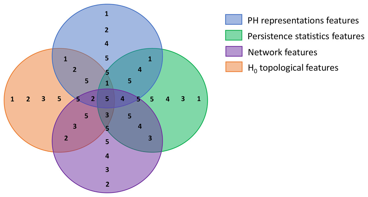
Figure 5: Venn diagram visualizing the swarm division strategy.
Each circle represents a solution space and the numbers within each space represent sub-swarm groups that search for optimal solution within that space. For example, sub-swarm group 1 does not appear in purple circle, which indicates that sub-swarm group 1 searches for optimal solution in the space that excluded network features.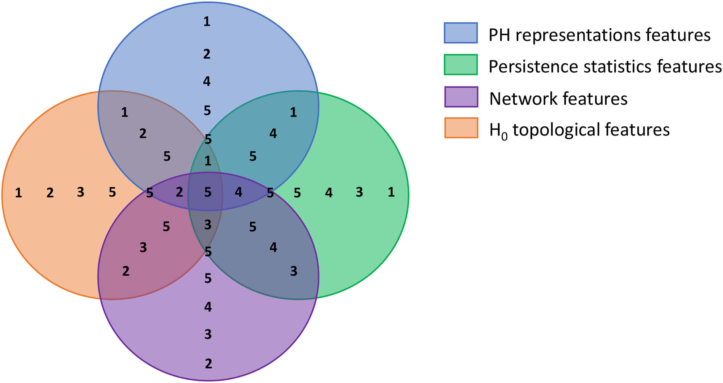
Improvement strategy 2: modified velocities update and clamping
After defining the population and sub-swarm sizes, the particles search for an optimal solution with the given velocity. We refined the velocity update strategy of our BPSO accordingly. Initially, we updated the particles’ velocity based on their personal best position and the global best position discovered by the whole swarm, as in Eq. (8). With the sub-swarm approach, we produced two global best positions, one by each sub-swarm (SSGbest), and one by the whole swarm as usual (SGbest). Thus, we modified the velocity update formula (Eq. (8)) to include the new sub-swarm global best, as shown in Eq. (12). This update method introduces greater diversity to the search for optimal solutions by particles. Moreover, we clamped the velocity of the particles within the range of to avoid overly rapid particle convergence.
(12)
Improvement strategy 3: dynamic inertia weight and acceleration coefficient
As in Eq. (10), we implemented a dynamic inertia weight that gradually decreases from 0.9 to 0.4 by iterations in our BPSO velocity update mechanism. This dynamic weight facilitates better particle search by letting the particles explore a broader area during early iterations and narrowing down the search area afterward. Similarly, we used dynamic acceleration coefficients in this study instead of the fixed coefficients in standard BPSO. We determined the value of our acceleration coefficients in every iteration with Eqs. (13) and (14). We set our to 2 and to 1. Higher at the beginning of the search enables the exploration of extensive space, while higher and in the subsequent search allow the particles to converge to the optimum.
(13)
(14)
Improvement strategy 4: worst solution enhancement with mutation and concatenation
All particles update their position (or solution) after the search in every iteration. Thus, our final improvement strategy is to further update the worst solutions with the mutated sub-swarm global best concatenation. In every three iterations, we identified the two weakest and one best particles in each sub-swarm, which are the particles that achieved the lowest and highest accuracy at that round. Then, we updated the position of the weakest particles with the concatenation of the best position in each sub-swarm. We enhanced a total of 10 particles (10% of the population) each time, and we further mutated the best position concatenation to ensure all 10 particles had different new positions.
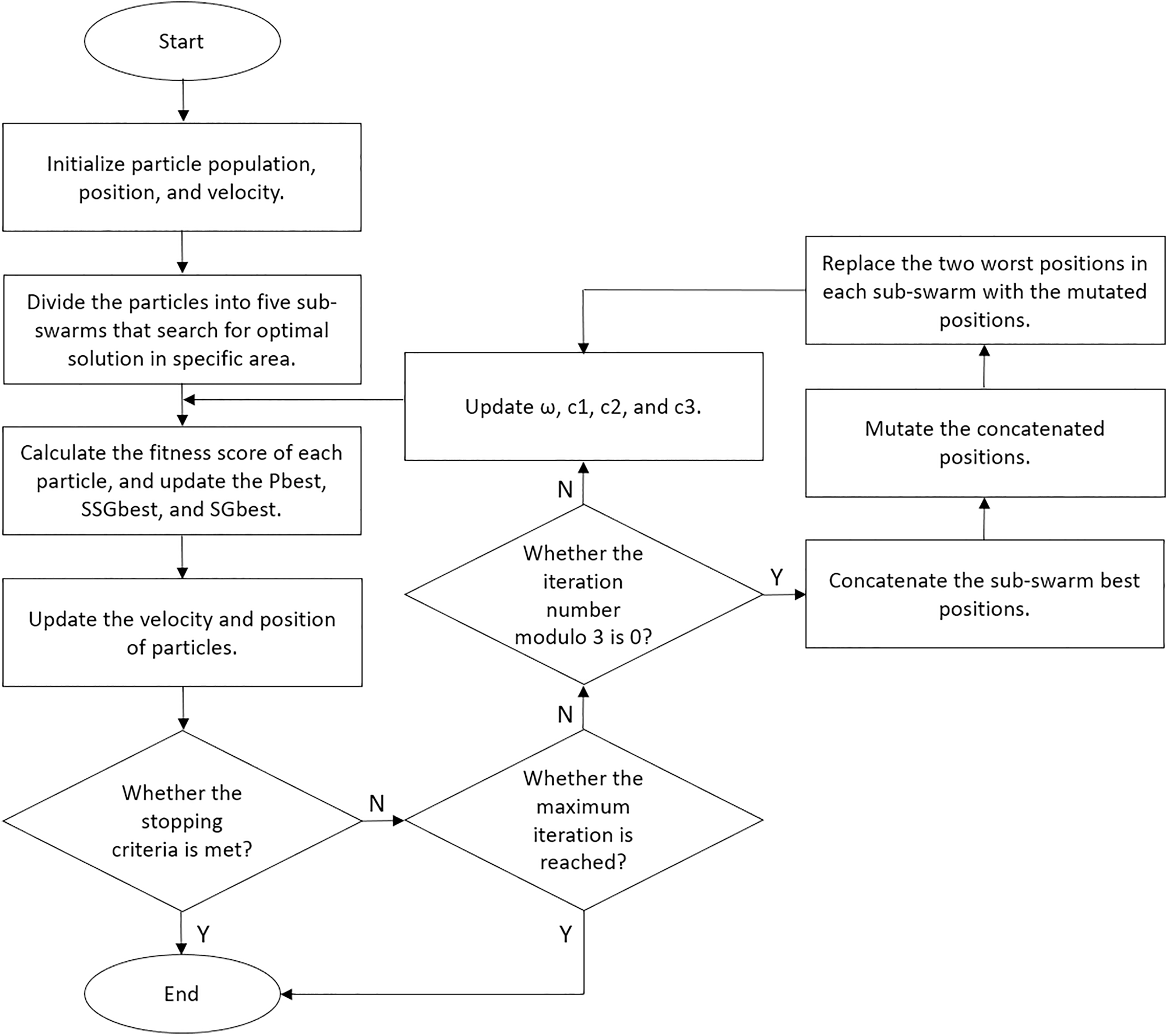
We set our BPSO to stop the search if the global best score increases by less than 1% after 10 iterations. Moreover, we implemented a fitness cache that records the fitness score of each solution, allowing the algorithm to retrieve scores for repeated solutions without reclassification. This approach reduces computational costs and enhances the efficiency of our BPSO. We performed five independent BPSO runs for each classification and obtained the feature subset that yielded the highest accuracy. We illustrated the details of our enhanced BPSO in Algorithm 1 and present a flowchart for the algorithm in Fig. 6.
| 1 Initialize a particle swarm of 100 particles, their positions and velocities |
| 2 Divide the swarm into 5 sub-swarms so that each sub-swarm search in a particular space |
| 3 Evaluate each particle and identify the Pbest, SSGbest, and SGbest |
| 4 for (k : Mk) do |
| 5 |
| 6 |
| 7 |
| 8 |
| 9 for (each sub-swarm a) do |
| 10 Select uniform random variable on the interval [0, 1] for r1, r2, and r3 |
| 11 for (each particle i) do |
| 12 Update velocity vi |
| 13 Update position xi |
| 14 Identify and update Pbest and SSGbest |
| 15 End |
| 16 End |
| 17 Identify and update SGbest |
| 18 if (stopping criteria met) then |
| 19 Stop the iteration |
| 20 End |
| 21 if (k % 3 = 0) then |
| 22 n←SSGbest concatenation |
| 23 for (each sub-swarm a) do |
| 24 Identify two worst particles |
| 25 for (each worst particle i) do |
| 26 Mutate n |
| 27 Update particle position with n |
| 28 End |
| 29 End |
| 30 End |
| 31 End |
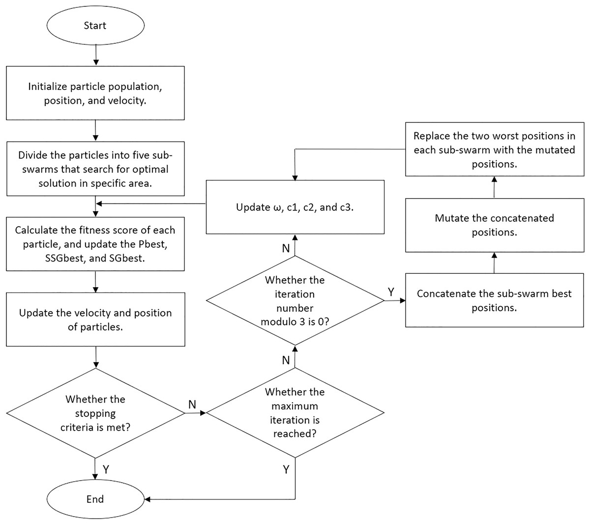
Figure 6: Flowchart of our enhanced BPSO.
We empirically determined the values of the hyperparameters for our enhanced BPSO, as shown in Table S1 in the Supplemental Information. We considered the appropriate trade-off between computational efficiency and the solution search effectiveness when selecting the hyperparameter values. We also performed a hyperparameter sensitivity analysis to evaluate how different hyperparameter values influence the classification performance and runtime.
Classification
In this study, we conducted binary EEG classification to distinguish between EEG recorded under quiet and distraction conditions by assuming that the effect of low and high sound distraction on EEG patterns has little to no differences. We employed four classifiers, namely logistic regression (LR), support vector machine (SVM), random forest (RF), and k-nearest neighbor (KNN). LR is a popular binary classifier that classifies input with a sigmoid function. SVM with radial basis kernel functions is powerful in separating non-linear data into classes. RF is a decision tree-based classifier that effectively handles large datasets with higher dimensionality. KNN classifies data based on their distance from their neighbors. We implemented these classifiers through the Python sklearn library (Pedregosa et al., 2011) and maintained the parameters’ default values except for LR maximum iterations (1,000) and KNN number of neighbors (3).
Before the classification, we standardized all extracted features by removing the mean and scaling to unit variance using the Python StandardScaler. We then conducted multiple experiments on single-trial EEG classification with various settings, as summarized in Table 4. Most experiments utilized VR filtration and WVG to extract features from alpha EEG signals. However, we alternated the type of VG and PH filtration methods in Experiments II and III respectively to compare their effectiveness. We applied the sliding window technique in Experiment IV to examine its impact on classification performance. Finally, we replaced alpha EEG with beta EEG in Experiment V to study how EEG in different frequency bands responds to surrounding noise.
| Experiment | Frequency band | Channel | Sliding window | PH filtration | VG |
|---|---|---|---|---|---|
| I | Alpha | T5, T6, O1, O2, OZ | ✗ | VR | WVG |
| II | Alpha | O2 | ✗ | VR | WVG, NVG, HVG, LPHVG |
| III | Alpha | OZ | ✗ | VR, sublevel set, graph | WVG |
| IV | Alpha | T5, O2 | ✓ | VR | WVG |
| V | Beta | T5, T6, O1, O2, OZ | ✗ | VR | WVG |
We employed the accuracy, precision, recall, and F1-score metrics to evaluate our classification results. We also applied the 5-fold cross-validation in our classification to ensure robust results. We implemented the PH and VG techniques using the Python Ripser (Tralie, Saul & Bar-On, 2018), Persim (Saul & Tralie, 2019), Gudhi, NetworkX (Hagberg, Swart & Schult, 2008), and ts2vg libraries.
To assess the significance of the features selected by our enhanced BPSO, we conducted a permutation test using the optimal feature sets that achieved the highest accuracy for each classifier. As a nonparametric method requiring minimal assumptions, permutation testing is particularly appropriate for topological descriptors (Sathyanarayana, Manjunath & Perea, 2025). Under the null hypothesis that the features used have no association with the class labels, we performed a 1,000-permutation test by randomly shuffling the class labels in each iteration. We chose the classification accuracy score as our test statistic and recorded the accuracy scores across the 1,000 classifications with permuted labeling. We then calculated the p-value of our test by dividing the number of significant permutations (i.e., the permutation that yielded a higher accuracy score than the original dataset) by the total number of permutations.
On the other hand, we also performed classification using the standard BPSO to compare its results with those from the enhanced BPSO classification. To assess the statistical significance of their differences, we first applied the Shapiro–Wilk test to examine the normality of the performance differences observed between standard and enhanced BPSO classifications across various classifiers. In the Shapiro–Wilk test, a p-value smaller than 0.05 indicates that the null hypothesis is rejected, where the result is not normally distributed. Then, we employed a parametric paired t-test for scenarios that show normality and a non-parametric Wilcoxon signed-rank test for the opposite. We selected these statistical test methods due to their strong statistical power, robustness, and effectiveness in the presence of outliers (Yavas et al., 2025).
Results
We begin this section by reporting the outcomes of our non-medical EEG classification experiments conducted under the settings outlined in Table 4. Each experiment was designed to evaluate different aspects of the proposed pipeline, including the classification performance across: (I) all selected channels with and without our feature selection technique, (II) features produced by different VG variants, and (III) different PH filtrations, (IV) the sliding window technique, (V) the alpha and beta signals. We then presented the results of our comparative analysis using medical EEG (i.e., Bonn dataset) for inspecting the generalizability of our methodologies. We conclude this section with a hyperparameter sensitivity analysis assessing the impact of two key parameters in our BPSO.
Experiment I: comparison of classification with complete and reduced features set
In our first experiment, we compared the performance of EEG classification using the complete feature set (i.e., the combination of PH representations, persistence statistics, and WVG features) against the reduced set selected through our enhanced BPSO. The classification was conducted separately for the five selected channels using single-trial alpha band EEG signals. From each of the 135 EEG time series (45 subjects × 3 conditions), we extracted 71 features to form a 135 × 71 feature matrix as input for the classification models.
We first explored the list of features selected by our enhanced BPSO for each classification (4 classifiers × 5 channels) in Table 5. For each channel, if none of the features in a particular category (PH representations, persistence statistics, or WVG features) are selected by a specific classifier, then the relevant row of that feature category is filled with “none”. Several features from PH representations are constantly selected, with exceptions for SVM with O1 and LR with O2 signals. Similarly, at least one of the WVG features is included, except for LR and RF with respective T5 and OZ signals. However, the persistence statistics are omitted in half of the classifications (see the row filled with “none” in the column of persistence statistics in Table 5). These findings indicate that PH representation and WVG effectively capture important information from nonlinear and nonstationary EEG signals better than persistence statistics.
| Channel | Classifier | Features selected (Number of features) | ||
|---|---|---|---|---|
| PH representations | Persistence statistics | Weighted VG | ||
| T5 | LR | f3, f6, f12, f21 (4) | f23–f25, f29, f30, f33, f37, f40, f42–f45, f48, f51, f53, f54, f57, f61 (18) | none |
| SVM | f2–f4, f10, f13, f15, f19–f21 (9) | none | f71 (1) | |
| RF | f7 (1) | f24, f28, f32, f35, f37, f42, f45, f50–f52, f57, f60–f62 (14) | f63 (1) | |
| KNN | f3, f4, f6–f8, f10 – f12, f15, f17, f18, f20, f22 (13) | none | f63, f64, f68, f69, f71 (5) | |
| T6 | LR | f1, f2, f6, f12, f13, f16–f20, f22 (11) | none | f65, f67, f71 (3) |
| SVM | f4, f7 , f9, f11, f19, f22 (6) | none | f64, f66 (2) | |
| RF | f7–f9, f22 (4) | none | f63, f64, f68, f69 (4) | |
| KNN | f3, f4, f7, f14, f22 (5) | f23, f24, f26, f28, f32, f35, f37, f40, f46, f50–f52, f55–f57, f62 (16) | f63, f65, f68–f70 (5) | |
| O1 | LR | f2, f4, f5, f7, f10, f13, f17, f21 (8) | none | f64, f65, f71 (3) |
| SVM | none | f26, f29, f55, f60 (4) | f63–f65, f68, f71 (5) | |
| RF | f3, f5–f9, f11, f15, f17, f19 (10) | none | f64, f66, f69, f71 (4) | |
| KNN | f4, f8, f13, f14, f17, f18, f21 (7) | f28, f32, f35, f37, f46, f47, f51, f52, f56, f62 (10) | f66, f71 (2) | |
| O2 | LR | none | f27–f29, f31, f40, f42, f54 (7) | f65 (1) |
| SVM | f10, f13, f16, f19, f20 (5) | none | f65, f66, f68 (3) | |
| RF | f7, f8, f10, f12–f15, f18 (8) | none | f63–f69, f71 (8) | |
| KNN | f8, f10, f13, f17, f18, f21 (6) | f24, f28, f30, f32, f35, f36, f40–f42, f50, f51, f60 (12) | f63, f65–f68, f71 (6) | |
| OZ | LR | f2, f4, f5, f7, f13, f15–f18, f21 (10) | f23–f25, f28, f32, f33, f36, f37, f40, f43, f45–f48, f53, f55, f56, f62 (18) | f65, f68, f70, f71 (4) |
| SVM | f3, f7, f14, f17, f18, f22 (6) | f28, f30, f32, f46, f50, f60 (6) | f63, f68, f71 (3) | |
| RF | f2, f3, f5, f7, f11, f12, f16, f17, f20 (9) | f23, f25–f27, f29, f34–f36, f38–f40, f44–f51 (19) | none | |
| KNN | f1, f3, f6, f11, f13, f14, f17 (7) | none | f65, f66, f71 (3) | |
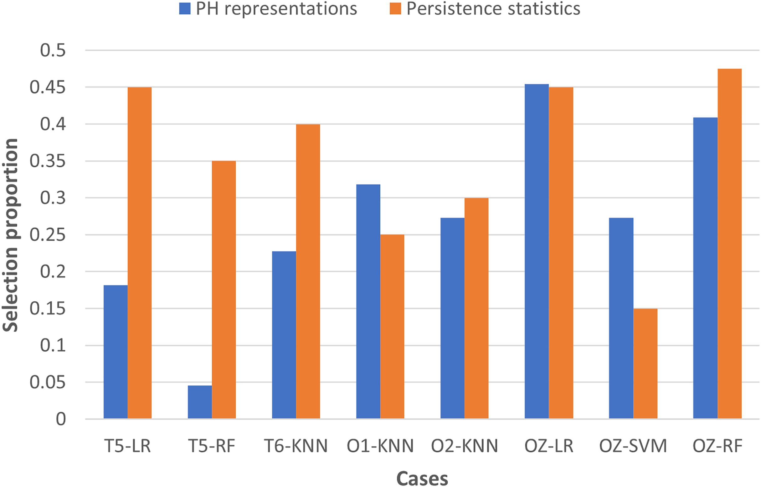
To examine the usefulness of persistence statistics in EEG classification, we analyzed the eight cases (i.e., LR and RF with T5 and OZ, SVM with OZ, and KNN with T6, O1, and O2) that include both PH representations and persistence statistics features in the classification by calculating their feature selection proportions (i.e., the ratio of the number of features selected to the total number of features in a particular category). The proportion facilitates the comparison of the number of features chosen across different categories, as we have different numbers of features in each category (i.e., 22 PH representations, 40 persistence statistics, and nine network features, as shown in Table 3).
Figure 7 shows that persistence statistics have a higher selection proportion, indicating that relatively more persistence statistics are chosen than the PH representation features in most of the eight cases (except KNN with O1 and SVM with OZ). This finding suggests that these statistics still offer strong discriminative power in the classification despite being omitted in many cases. On the other hand, some PH representation features might be redundant and carry less essential topological information in particular cases. However, it is noteworthy that the combination of PH representations and WVG features is generally sufficient for the classification models to reach optimal performance in the remaining cases. Thus, the persistence statistics act more like a complementary feature in this experiment.
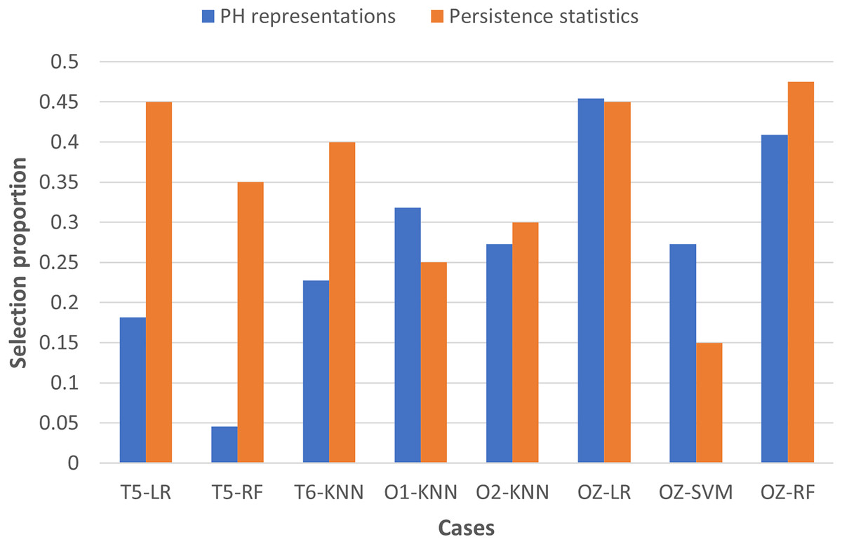
Figure 7: Bar chart comparing the feature selection proportion between PH representations and persistence statistics.
After applying feature selection, we compared the classification results between complete and reduced feature sets across all channels and classifiers in Table 6. Accompanied by Table 6, Fig. 8 gives the accuracy and F1-score increments achieved in Table 6 across different classifiers. The highest accuracy and F1-score improvements obtained from LR are 16.30% and 14.83% with O1 and T6 signals, respectively. SVM yields the highest accuracy (3.7%) and F1-score (2.06%) gains with OZ signals. Meanwhile, RF achieves the highest accuracy (15.56%) and F1-score (11.16%) increments with OZ signals. KNN with O2 signals gives the highest accuracy (23.71%) and F1-score (17.77%) increments. These suggest that our enhanced BPSO reliably excludes redundant and weakly informative features, resulting in improved classification performance across all channels and classifiers.
| Channel | Classifier | Feature set | Accuracy | Precision | Recall | F1 |
|---|---|---|---|---|---|---|
| T5 | LR | Complete | 56.30 | 66.02 | 74.62 | 68.66 |
| Reduced | 71.85 | 72.71 | 94.49 | 81.10 | ||
| SVM | Complete | 66.67 | 66.67 | 100 | 79.30 | |
| Reduced | 70.37 | 69.04 | 100 | 81.09 | ||
| RF | Complete | 65.19 | 70.07 | 85.20 | 75.78 | |
| Reduced | 74.81 | 74.70 | 94.46 | 82.66 | ||
| KNN | Complete | 60.00 | 68.85 | 78.21 | 71.74 | |
| Reduced | 74.81 | 77.11 | 88.24 | 81.85 | ||
| T6 | LR | Complete | 54.07 | 64.84 | 68.88 | 65.55 |
| Reduced | 69.63 | 69.08 | 97.80 | 80.38 | ||
| SVM | Complete | 66.67 | 66.67 | 100 | 79.30 | |
| Reduced | 68.15 | 67.66 | 100 | 80.01 | ||
| RF | Complete | 54.81 | 62.63 | 83.13 | 70.27 | |
| Reduced | 68.15 | 72.15 | 90.22 | 78.54 | ||
| KNN | Complete | 57.04 | 64.50 | 76.80 | 69.60 | |
| Reduced | 71.85 | 75.45 | 88.02 | 80.22 | ||
| O1 | LR | Complete | 53.33 | 64.48 | 75.85 | 67.86 |
| Reduced | 69.63 | 69.02 | 98.82 | 80.54 | ||
| SVM | Complete | 66.67 | 66.67 | 100 | 79.30 | |
| Reduced | 67.41 | 67.66 | 99.13 | 79.58 | ||
| RF | Complete | 58.52 | 64.47 | 81.63 | 71.23 | |
| Reduced | 67.41 | 69.82 | 91.8 | 78.44 | ||
| KNN | Complete | 58.52 | 66.08 | 75.16 | 69.72 | |
| Reduced | 73.33 | 74.49 | 91.21 | 81.31 | ||
| O2 | LR | Complete | 58.52 | 66.21 | 76.40 | 70.09 |
| Reduced | 70.37 | 69.98 | 96.83 | 80.63 | ||
| SVM | Complete | 66.67 | 66.67 | 100 | 79.30 | |
| Reduced | 68.15 | 67.92 | 100 | 80.05 | ||
| RF | Complete | 57.04 | 67.64 | 75.14 | 69.45 | |
| Reduced | 71.11 | 71.99 | 93.12 | 80.40 | ||
| KNN | Complete | 52.59 | 64.26 | 70.23 | 65.85 | |
| Reduced | 76.30 | 76.04 | 95.02 | 83.62 | ||
| OZ | LR | Complete | 62.96 | 69.86 | 82.95 | 74.28 |
| Reduced | 71.85 | 72.49 | 94.96 | 81.19 | ||
| SVM | Complete | 65.93 | 66.38 | 98.82 | 78.73 | |
| Reduced | 69.63 | 69.06 | 100 | 80.79 | ||
| RF | Complete | 53.33 | 64.12 | 74.57 | 67.48 | |
| Reduced | 68.89 | 72.14 | 89.36 | 78.64 | ||
| KNN | Complete | 54.07 | 64.65 | 71.68 | 66.86 | |
| Reduced | 70.37 | 74.20 | 85.06 | 78.79 |
Note:
The bold values indicate the highest accuracy and F1-score achieved by each classifier.
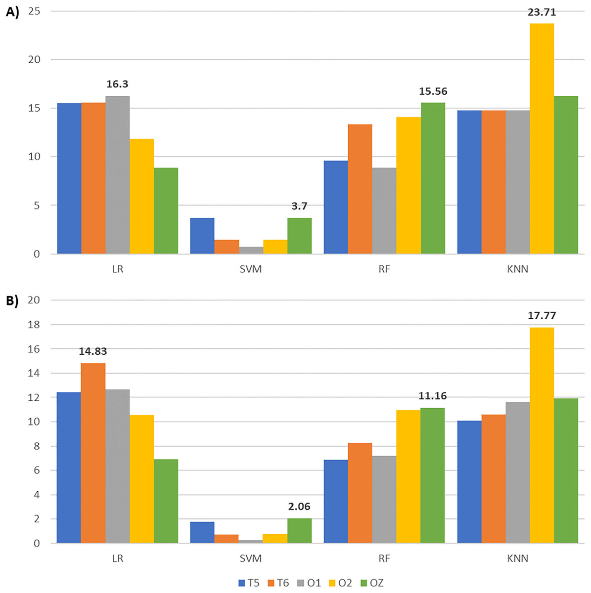
Figure 8: Bar charts illustrating the metric scores increments across classifiers and channels with the highest increments shown above the bars.
(A) The accuracy and (B) the F1-score increments achieved by comparing the EEG classification with enhanced BPSO and without feature selection.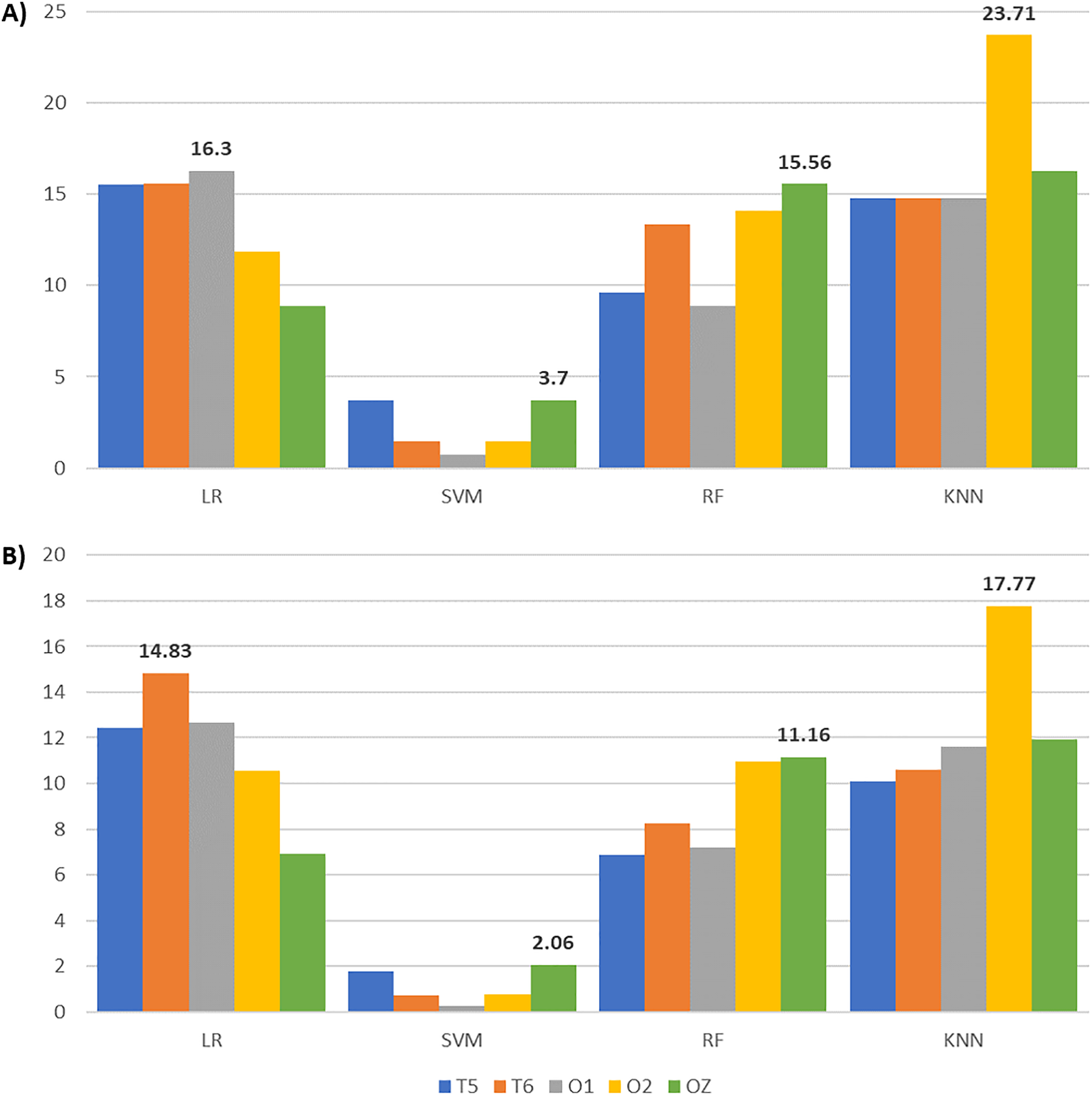
Although Fig. 8 indicates that EEG signals from channel T5 do not yield the highest accuracy and F1-score improvement under any classifier, Table 6 reveals that T5 constantly gives the highest accuracy for reduced feature sets across classifiers, except for KNN. A possible explanation for the modest accuracy gain with T5 is that its performance with the complete feature set already outperformed that of the other channels, leaving limited room for further improvement. When focusing on the reduced feature set, T5 produces the highest accuracy for LR (71.85%), SVM (70.37%), and RF (74.81%), with corresponding F1-scores of 81.10%, 81.09%, and 82.66%. For KNN, T5 achieves 74.81% accuracy and an 81.85% F1-score, slightly below the highest scores of 76.30% and 83.62% obtained with O2. These results suggest that features extracted from T5 effectively distinguish EEG signals across auditory conditions, highlighting the sensitivity of the left temporal brain region to surrounding noise.
Besides the overall metric scores reported, we also computed the per-class precision, recall, F1-score, and precision-recall area under the curve (PR-AUC) for alpha T5 and O2 EEG, which yielded the highest classification performance across classifiers. We presented the results in Table S2 and constructed confusion matrices for these classifications in Figs. S1 in the Supplemental Information. Both the low recall and F1-scores for class 0 (i.e., quiet condition), along with the patterns in the confusion matrices, indicate that our classification framework is biased towards classifying distraction EEG, likely due to the class imbalance in our dataset. The results also suggest that distracted EEG with increased alpha and beta activity (Kuang et al., 2024) may generate more distinguishable topological features, leading to higher performance than quiet EEG.
We further computed the permutation importance of the features used in each T5 classification to study the feature contributions in improving the classification. Specifically, we permutated the values of a given feature and assessed the model’s performance over 30 times. Permuting features with high importance will cause a significant performance drop when compared to the model with the original feature. The feature importance plots in Fig. S2 in the Supplemental Information reveal that persistence statistics and landscape consistently rank among the top three most important across all classifiers, except KNN. For KNN classification, the top three features are all network features, including degree assortativity (f71), which were frequently selected across multiple cases in Table 5. These features effectively capture the discriminative topological structure of the EEG and improve the classification results.
In addition, we compared the classifications between the standard and our enhanced BPSO in Table S3 of the Supplemental Information. Our enhanced BPSO produced accuracy and F1-score matching or exceeding the standard BPSO in most cases, except the F1-score from the classification of T5 signal with KNN. This finding suggests that our proposed BPSO outperforms the standard BPSO in classifying EEG recorded under different auditory conditions. We also reported in Table S4 the permutation test results for the four scenarios that achieved the highest accuracy scores with each classifier. The p-values acquired are lower than 0.01 for every classification, indicating that the likelihood of observing such a high accuracy with the selected features purely by chance is less than 1%.
We conducted statistical tests to determine whether the performance differences between the enhanced BPSO, the standard BPSO, and no feature selection were statistically significant across various classifiers. We first checked the normality using the Shapiro–Wilk test (see Table S5). We then performed a paired t-test for cases with a Shapiro–Wilk test result greater than 0.05 and a Wilcoxon signed-rank test for the remaining cases. Table 7 shows the results of the statistical tests. In the direct comparison between the enhanced and standard BPSO, only SVM and RF classifiers yielded p-value less than 0.05 for the accuracy score, suggesting that the observed accuracy differences between these two BPSO are statistically significant for these classifiers. However, the p-values obtained for LR and KNN classifiers exceed 0.05, indicating no significant difference. This lack of significance may be attributed to the high variability in their pairwise accuracy differences (Arévalo-Cordovilla & Peña, 2025). Although the enhanced BPSO achieved statistically significant accuracy improvements over the standard BPSO only for SVM and RF, its comparison with classification without applying any feature selection revealed consistently lower p-values across most classifiers and metrics. This finding suggests that the enhanced BPSO provides greater and more consistent improvements than the standard BPSO, even when statistical significance is not always observed in their direct comparisons.
| Classifier | Classification | p-value (Wilcoxon/Paired t-test) | |||
|---|---|---|---|---|---|
| Accuracy | Precision | Recall | F1-score | ||
| LR | Enhanced vs Standard | 0.303 | 0.666 | 0.008 | 0.118 |
| Enhanced vs None | 1.30 × 10⁻⁷ | 2.00 × 10⁻⁴ | 4.51 × 10⁻⁹ | 3.42 × 10⁻⁸ | |
| Standard vs None | 3.46 × 10⁻⁵ | 1.30 × 10⁻⁵ | 9.83 × 10⁻⁹ | 3.09 × 10⁻⁵ | |
| SVM | Enhanced vs Standard | 0.010 | 0.007 | 0.317 | 0.011 |
| Enhanced vs None | 1.28 × 10⁻³ | 9.48 × 10⁻⁴ | 0.655 | 0.001 | |
| Standard vs None | 0.026 | 0.028 | 0.317 | 0.028 | |
| RF | Enhanced vs Standard | 0.032 | 0.051 | 0.185 | 0.051 |
| Enhanced vs None | 2.17 × 10⁻⁷ | 5.81 × 10⁻⁶ | 4.65 × 10⁻⁵ | 7.08 × 10⁻⁷ | |
| Standard vs None | 1.10 × 10⁻⁶ | 4.01 × 10⁻⁵ | 4.37 × 10⁻⁴ | 4.01 × 10⁻⁵ | |
| KNN | Enhanced vs Standard | 0.177 | 0.031 | 0.522 | 0.194 |
| Enhanced vs None | 1.15 × 10⁻⁸ | 1.02 × 10⁻⁷ | 2.40 × 10⁻⁶ | 4.56 × 10⁻⁸ | |
| Standard vs None | 5.28 × 10⁻⁹ | 3.43 × 10⁻⁷ | 7.67 × 10⁻⁶ | 8.37 × 10⁻⁸ | |
Note:
The bold p-values are lower than 0.05, suggesting the score difference of the corresponding classifications is statistically significant.
Experiment II: comparison of classification with different visibility graph techniques
In “Materials and Methods”, we have seen that different VG techniques convert time series into graphs using distinct strategies. Although this can capture varying characteristics of EEG time series, it may impact classification performance. To investigate this, we applied three different VG techniques (namely HVG, NVG, LPHVG) to our EEG data, extracted their corresponding features, and compared the classification results with those from the first experiment using WVG features. We focused on the O2 classification as it yielded relatively high accuracy across classifiers with network features constantly selected for optimal performance (see Tables 5 and 6).
Table 8 summarizes the EEG classification results using different VG techniques with O2 signals. Features extracted from WVG constantly yield the highest classification accuracy, followed by HVG, NVG, and LPHVG, regardless of the classifier used. WVG differs from the other VGs by assigning weight to each edge, capturing both the data points’ connectivity and amplitude dynamics, and allowing the classifier to distinguish between patterns that might appear similar when connectivity is the only consideration. Despite being computationally efficient, HVG, NVG, and LPHVG focus solely on connectivity, leading to a loss of finer quantitative details in the signal.
| Classifier | Visibility graph | Accuracy | Precision | Recall | F1 |
|---|---|---|---|---|---|
| LR | WVG | 70.37 | 69.98 | 96.83 | 80.63 |
| HVG | 68.89 | 69.57 | 94.37 | 79.41 | |
| NVG | 68.15 | 68.61 | 93.78 | 78.79 | |
| LPHVG | 68.15 | 68.68 | 96.83 | 79.53 | |
| SVM | WVG | 68.15 | 67.92 | 100 | 80.05 |
| HVG | 67.41 | 67.32 | 100 | 79.67 | |
| NVG | 67.41 | 67.32 | 100 | 79.67 | |
| LPHVG | 67.41 | 67.32 | 100 | 79.67 | |
| RF | WVG | 72.59 | 73.84 | 92.89 | 81.29 |
| HVG | 71.85 | 71.71 | 95.75 | 81.27 | |
| NVG | 71.11 | 72.69 | 88.79 | 79.34 | |
| LPHVG | 68.15 | 70.93 | 90.47 | 78.49 | |
| KNN | WVG | 76.30 | 76.04 | 95.02 | 83.62 |
| HVG | 75.56 | 77.84 | 89.08 | 82.36 | |
| NVG | 68.89 | 74.42 | 84.05 | 77.7 | |
| LPHVG | 68.89 | 73.24 | 84.77 | 77.79 |
Note:
The bold values indicate the highest accuracy score achieved by each classifier.
Apart from comparing the classification performance across different VG techniques, we also examined which network features listed in Table 2 are worth considering using our enhanced BPSO. Table 9 enumerates the features selected in each VG technique across different classifiers for O2 signal classification. The most frequently chosen feature is modularity (10 times), followed by transitivity (eight times), with density and global efficiency selected six times. In contrast, the average weighted degree and clustering coefficient appear least often (three times). This variation suggests that some network features have greater discriminative power for EEG classification. Features such as average weighted shortest path length and modularity that respectively capture the flow of information and global community structure effectively summarize the complex spatiotemporal dynamics inherent in EEG signals. Conversely, metrics like average weighted degree and clustering coefficient focus more on local connectivity and may not differentiate the underlying brain states as robustly.
| Classifier | Graphs | AWD1 | AWSPL2 | MOD3 | DEN4 | TRAN5 | LE6 | GE7 | ACC8 | DA9 |
|---|---|---|---|---|---|---|---|---|---|---|
| LR | WVG | ✗ | ✗ | ✓ | ✗ | ✗ | ✗ | ✗ | ✗ | ✗ |
| HVG | ✗ | ✗ | ✗ | ✗ | ✓ | ✗ | ✗ | ✗ | ✗ | |
| NVG | ✗ | ✗ | ✓ | ✗ | ✗ | ✗ | ✗ | ✓ | ✓ | |
| LPHVG | ✗ | ✓ | ✗ | ✗ | ✓ | ✓ | ✗ | ✓ | ✗ | |
| SVM | WVG | ✗ | ✗ | ✓ | ✗ | ✗ | ✓ | ✗ | ✗ | ✓ |
| HVG | ✗ | ✗ | ✓ | ✓ | ✓ | ✗ | ✓ | ✗ | ✗ | |
| NVG | ✗ | ✗ | ✓ | ✓ | ✗ | ✓ | ✗ | ✗ | ✗ | |
| LPHVG | ✗ | ✗ | ✗ | ✓ | ✗ | ✗ | ✓ | ✗ | ✗ | |
| RF | WVG | ✗ | ✗ | ✓ | ✗ | ✓ | ✓ | ✓ | ✗ | ✗ |
| HVG | ✓ | ✓ | ✓ | ✗ | ✗ | ✗ | ✗ | ✗ | ✗ | |
| NVG | ✓ | ✗ | ✓ | ✓ | ✗ | ✗ | ✓ | ✗ | ✗ | |
| LPHVG | ✗ | ✓ | ✗ | ✗ | ✓ | ✗ | ✗ | ✗ | ✓ | |
| KNN | WVG | ✓ | ✗ | ✓ | ✓ | ✓ | ✓ | ✓ | ✗ | ✗ |
| HVG | ✗ | ✓ | ✓ | ✗ | ✓ | ✗ | ✗ | ✗ | ✗ | |
| NVG | ✗ | ✗ | ✗ | ✓ | ✗ | ✗ | ✗ | ✓ | ✓ | |
| LPHVG | ✗ | ✗ | ✗ | ✗ | ✓ | ✗ | ✓ | ✗ | ✓ |
Note:
1AWD = Average weighted degree; 2AWSPL = Average weighted shortest path length; 3MOD = Modularity; 4DEN = Density; 5TRAN = Transitivity; 6LE = Local efficiency; 7GE = Global efficiency; 8ACC = Average clustering coefficient; 9DA = Degree assorativity.
Experiment III: comparison of classification with different filtrations in persistent homology
Besides the variety in VG construction, different filtrations exist for constructing PH. In our third experiment, we constructed PH for our EEG data through different filtrations, including the VR, sublevel set, and graph filtration, and compared their classification results. Each filtration generates distinct PDs and topological features, potentially influencing classification accuracy. We focused on the classifications with OZ since PH representations and persistence statistics features are constantly selected in these cases (see Table 5).
Table 10 presents the classification results of OZ signals using topological features from different PH filtrations. For LR and SVM, VR filtration features achieve the highest accuracy, while sublevel and graph filtration features yield similarly lower scores. In contrast, RF and KNN perform better with sublevel filtration. Generally, VR and sublevel filtration features constantly produce the highest accuracy, whereas graph filtration performs less well than the others.
| Classifier | PH filtration | Accuracy | Precision | Recall | F1 |
|---|---|---|---|---|---|
| LR | VR | 71.11 | 73.65 | 91.45 | 80.30 |
| Sublevel | 68.89 | 69.44 | 95.71 | 79.71 | |
| Graph | 68.89 | 70.74 | 93.61 | 79.38 | |
| SVM | VR | 69.63 | 69.06 | 100 | 80.79 |
| Sublevel | 67.41 | 67.72 | 97.71 | 79.27 | |
| Graph | 67.41 | 66.73 | 100 | 79.67 | |
| RF | VR | 68.89 | 72.14 | 89.36 | 78.64 |
| Sublevel | 74.81 | 77.94 | 90.52 | 82.35 | |
| Graph | 69.63 | 73.82 | 86.81 | 78.65 | |
| KNN | VR | 70.37 | 74.20 | 85.06 | 78.79 |
| Sublevel | 72.59 | 76.02 | 86.84 | 80.16 | |
| Graph | 69.63 | 74.19 | 83.29 | 77.65 |
Note:
The bold values indicate the highest accuracy score achieved by each classifier.
As VR filtration constructs simplicial complexes based on distance thresholds in a time-delay embedded data cloud, it effectively captures the signal’s global structure and periodicity. Their associated features may be more linearly separable, and therefore, linear classifiers like LR and SVM can achieve higher accuracy with these features. In contrast, sublevel set filtration extracts topological features directly from the EEG amplitude, which is unavoidably sensitive to nonlinearity and transient local fluctuations in the signal. As a result, non-linear classifiers such as RF and KNN perform better with sublevel filtration features. Meanwhile, graph filtration may lose some discriminative detail during the discretization or matrix transformation, leading to relatively lower classification accuracy for most of the classifiers in Experiment III. Additionally, graph filtration primarily captures local connectivity and lacks the flexibility to reflect dynamic brain network changes over time (Bhattacharya et al., 2025).
Apart from comparing the classification accuracy across different filtrations, we also investigated which PH representations are most relevant for OZ classification using our enhanced BPSO. Table 11 shows the topological features of H0 and H1 selected by our enhanced BPSO for each PH representation in OZ classification across different classifiers and filtrations. Notably, sublevel set filtration differs from the other filtrations as it only produces H0 topological features (see the dashes in all H1 columns for sublevel rows in Table 11). As for PH representation features, persistence landscape shows strong discriminative power and is chosen most frequently, followed by persistence silhouette, persistence image, and Betti curve features. However, persistence entropy features are not being selected at all. This suggests that persistence entropy features might have minimal influence on classification for our EEG time series. The importance of persistence entropy features is even less than persistence statistics. Similar to Experiment I, nearly half of the persistence statistics features are omitted in this OZ classification. Even so, persistence statistics are the sole features being selected in the graph filtration for LR and RF classifiers. Results from Table 11 also suggest that H0 topological features carry valuable information comparable to H1 topological features except they are consistently excluded in VR filtration using SVM classifier.
| Classifier | PH filtration | PL1 | PE2 | PI3 | PS4 | BC5 | STAT6 | ||||||
|---|---|---|---|---|---|---|---|---|---|---|---|---|---|
| H0 | H1 | H0 | H1 | H0 | H1 | H0 | H1 | H0 | H1 | H0 | H1 | ||
| LR | VR | ✓ | ✓ | ✗ | ✗ | ✗ | ✓ | ✓ | ✓ | ✗ | ✓ | ✓ | ✓ |
| Sublevel | ✓ | – | ✗ | – | ✓ | – | ✗ | – | ✗ | – | ✗ | – | |
| Graph | ✗ | ✗ | ✗ | ✗ | ✗ | ✗ | ✗ | ✗ | ✗ | ✗ | ✓ | ✓ | |
| SVM | VR | ✗ | ✓ | ✗ | ✗ | ✗ | ✓ | ✗ | ✓ | ✗ | ✓ | ✗ | ✓ |
| Sublevel | ✓ | – | ✗ | – | ✗ | – | ✓ | – | ✗ | – | ✗ | – | |
| Graph | ✓ | ✓ | ✗ | ✗ | ✓ | ✗ | ✓ | ✓ | ✗ | ✗ | ✗ | ✗ | |
| RF | VR | ✓ | ✓ | ✗ | ✗ | ✓ | ✗ | ✓ | ✓ | ✓ | ✗ | ✓ | ✓ |
| Sublevel | ✓ | – | ✗ | – | ✓ | – | ✓ | – | ✓ | – | ✓ | – | |
| Graph | ✗ | ✗ | ✗ | ✗ | ✗ | ✗ | ✗ | ✗ | ✗ | ✗ | ✓ | ✓ | |
| KNN | VR | ✓ | ✓ | ✗ | ✗ | ✓ | ✓ | ✗ | ✓ | ✗ | ✗ | ✗ | ✗ |
| Sublevel | ✗ | – | ✗ | – | ✗ | – | ✗ | – | ✗ | – | ✓ | – | |
| Graph | ✓ | ✓ | ✗ | ✗ | ✗ | ✗ | ✓ | ✓ | ✗ | ✓ | ✗ | ✗ | |
Note:
1PL = Persistence landscape; 2PE = Persistence entropy; 3PI = Persistence image; 4PS = Persistence silhouette; 5BC = Betti curve; 6STAT = Persistence statistics.
Experiment IV: comparison of classification with and without segmentation
In our fourth experiment, we repeated the EEG classification by applying a 250 Hz non-overlapping sliding window to investigate its impact on classification performance. We focused on the T5 and O2 classifications, which provide the highest accuracy score for each classifier among all channels. With sliding window segmentation, we doubled our data size from 135 to 270 time series.
Figure 9 compares T5 and O2 classification results with and without sliding windows. For T5, the classification without a sliding window consistently achieves higher accuracy and F1-score across all classifiers. Similarly, for O2, the classification without a sliding window outperforms the classification with a sliding window, except for the SVM F1-score with a minimal difference (80.05% vs 80.49%). Given this negligible variation, the sliding window approach has minor impact on the classification performance with our EEG data. The findings may be attributed to our relatively short EEG time series (with only 512 Hz or 512 data points). Segmentation may disrupt the time series intrinsic pattern and reduce their temporal correlations, especially when the time series is short.
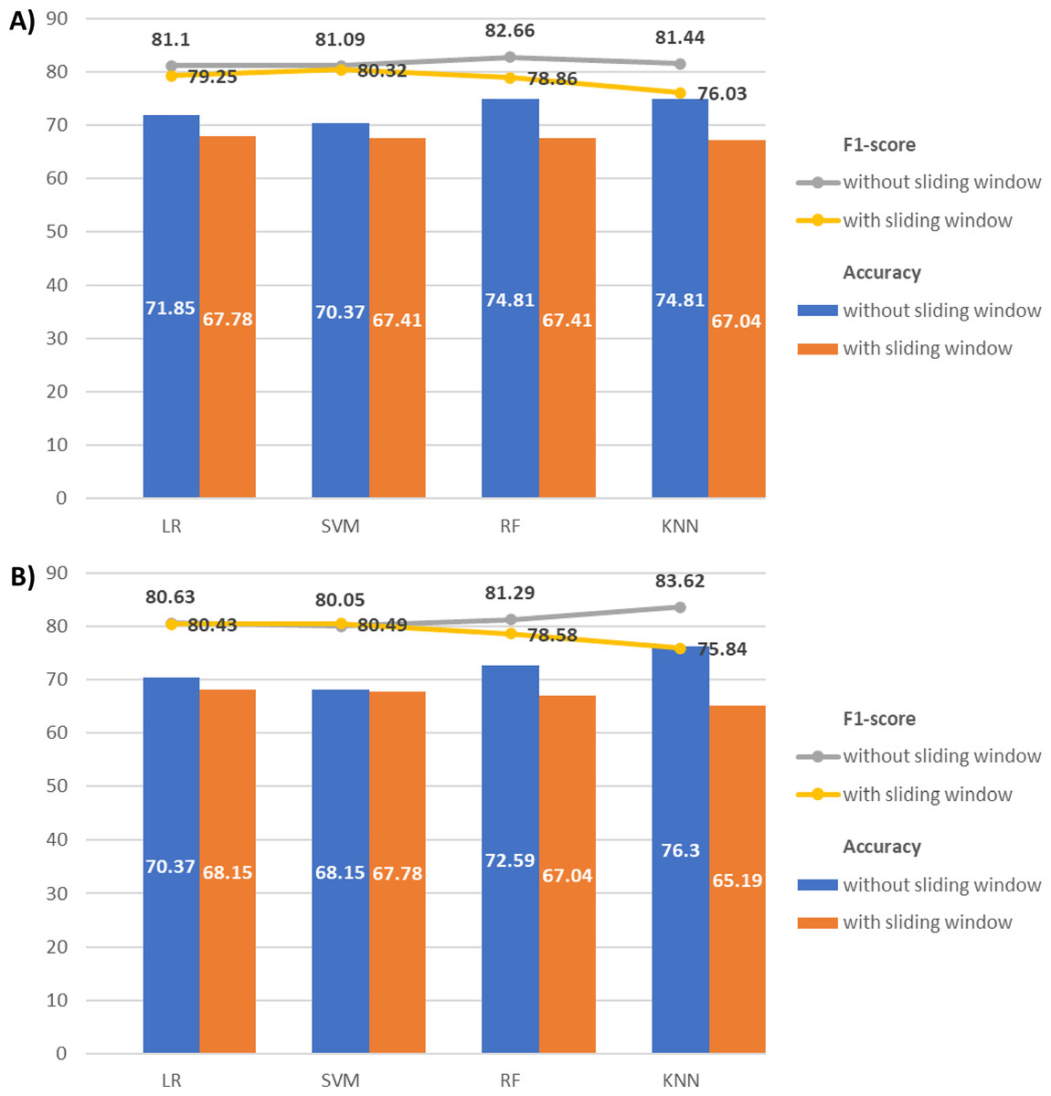
Figure 9: Combination of line and bar charts that illustrates the accuracy and F1-score of EEG classification with and without applying sliding window.
(A) The EEG classification results with T5 and (B) O2 signals.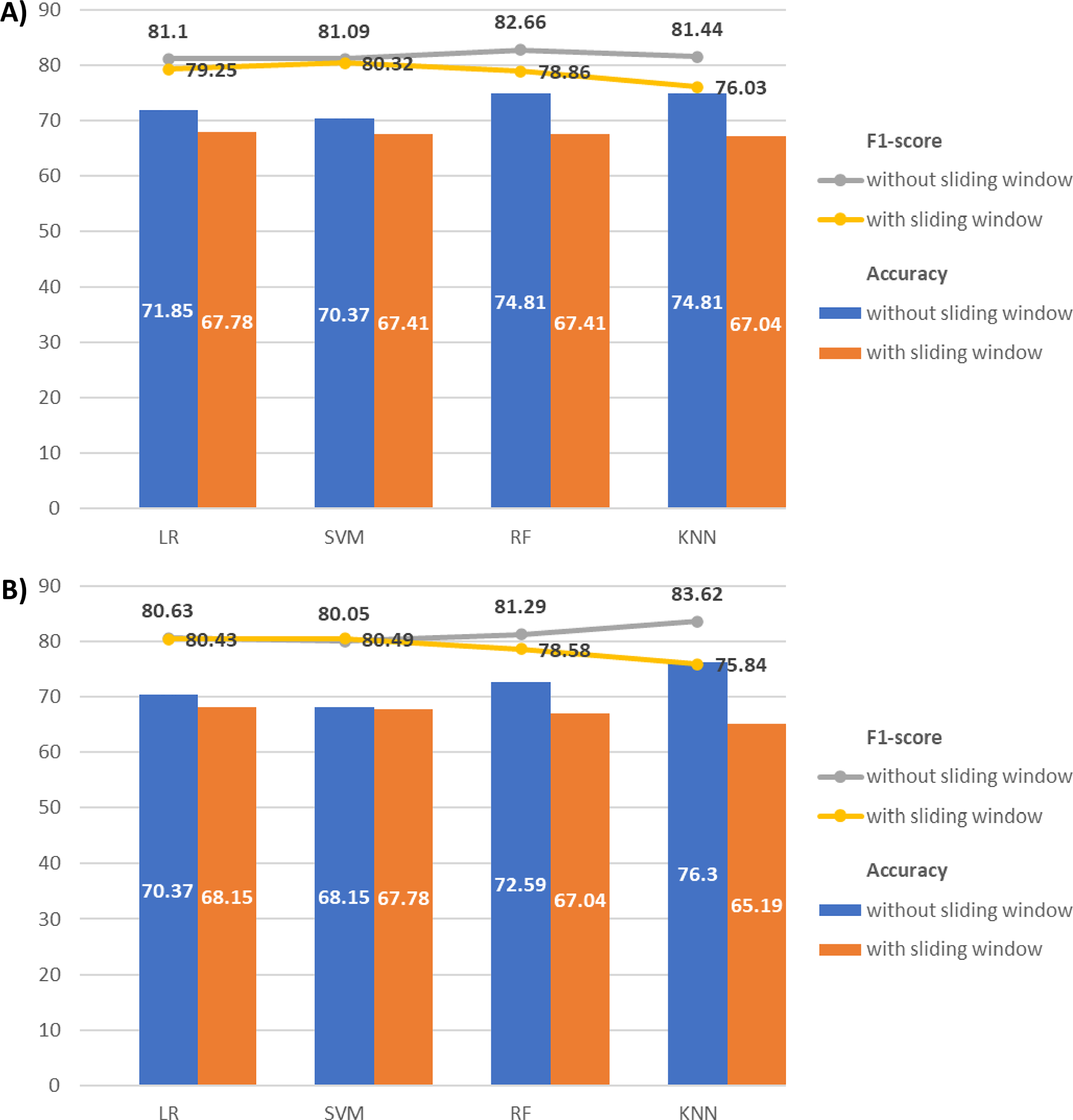
Experiment V: comparison of classification with different frequency bands EEG
In our last experiment, we conducted the EEG classification using beta-band EEG signals. For clarity, we only discuss the T5 and O2 beta EEG classification in this section and present the classification results of the other channels in Table S6 (Supplemental Information). We first showed the results of classifying T5 and O2 signals with complete and reduced feature sets, in Table 12. Similar to the results of alpha-band EEG signals in Experiment I (see Table 6), the enhanced BPSO effectively selects the optimal features and enhances classification performance for beta-band signals across classifiers, except for SVM with T5, which gives the same results regardless of the feature set.
| Channel | Classifier | Feature set | Accuracy | Precision | Recall | F1 |
|---|---|---|---|---|---|---|
| T5 | LR | Complete | 64.44 | 67.64 | 88.33 | 75.92 |
| Reduced | 70.37 | 70.04 | 97.62 | 80.76 | ||
| SVM | Complete | 66.67 | 66.67 | 100 | 79.30 | |
| Reduced | 66.67 | 66.67 | 100 | 79.30 | ||
| RF | Complete | 61.48 | 66.22 | 88.23 | 74.71 | |
| Reduced | 71.11 | 72.36 | 94.93 | 80.86 | ||
| KNN | Complete | 51.11 | 61.72 | 72.61 | 65.78 | |
| Reduced | 68.15 | 73.21 | 83.58 | 77.23 | ||
| O2 | LR | Complete | 58.52 | 65.92 | 78.09 | 70.74 |
| Reduced | 70.37 | 71.87 | 89.77 | 79.21 | ||
| SVM | Complete | 65.19 | 66.43 | 98.26 | 78.40 | |
| Reduced | 67.41 | 67.54 | 99.05 | 79.54 | ||
| RF | Complete | 59.26 | 65.98 | 79.83 | 71.37 | |
| Reduced | 69.63 | 70.57 | 92.43 | 79.56 | ||
| KNN | Complete | 56.30 | 64.99 | 71.77 | 67.39 | |
| Reduced | 68.89 | 75.34 | 79.34 | 76.68 |
We then compared the classification results across frequency bands to assess their discriminative power and validate our feature selection approach. Figures 10A and 10B depict the accuracy and F1-score improvements with feature selection via our enhanced BPSO for alpha and beta signal classifications. Generally, the increments of the classification scores in alpha signals are higher than or close to those of their corresponding beta signals. This finding suggests that the alpha signal may respond more actively to the surrounding noises than the beta signal. The only exceptions are in the T5 signals with KNN and O2 signals with SVM, where the respective beta signals achieve higher accuracy (17.04% and 2.22% against 14.81% and 1.48%) and F1-score (11.45% and 1.14% against 10.11% and 0.75%) increments than alpha signals. Notably, the largest performance boost from enhanced BPSO is recorded in alpha O2 signals using KNN, increasing accuracy by 23.71% and F1-score by 17.77%.
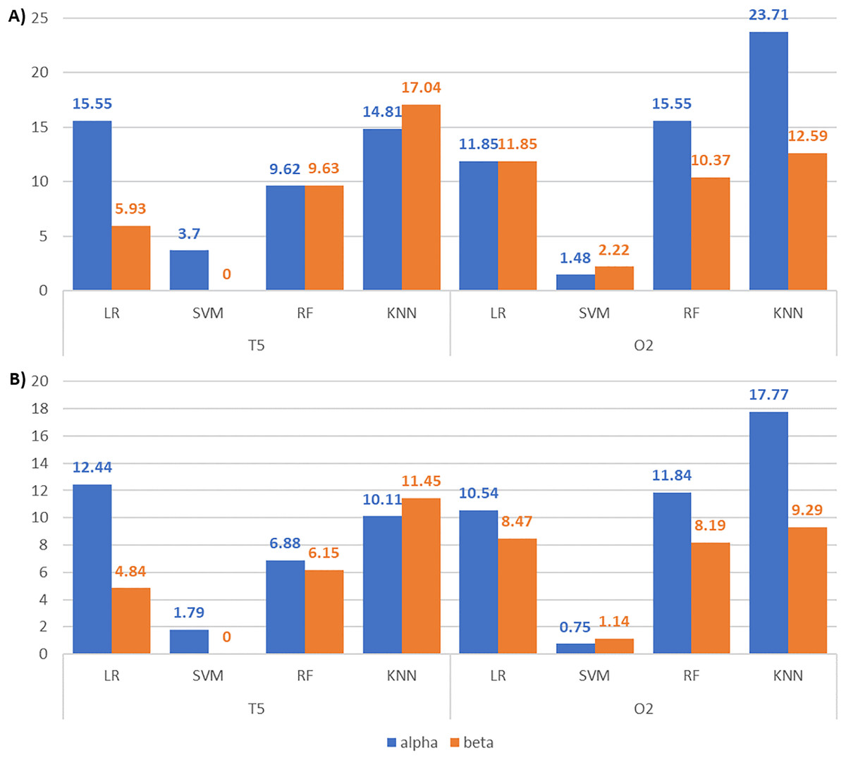
Figure 10: Bar charts illustrating the metric scores increments between the alpha and beta T5 and O2 EEG classifications.
(A) The accuracy and (B) the F1-score increments.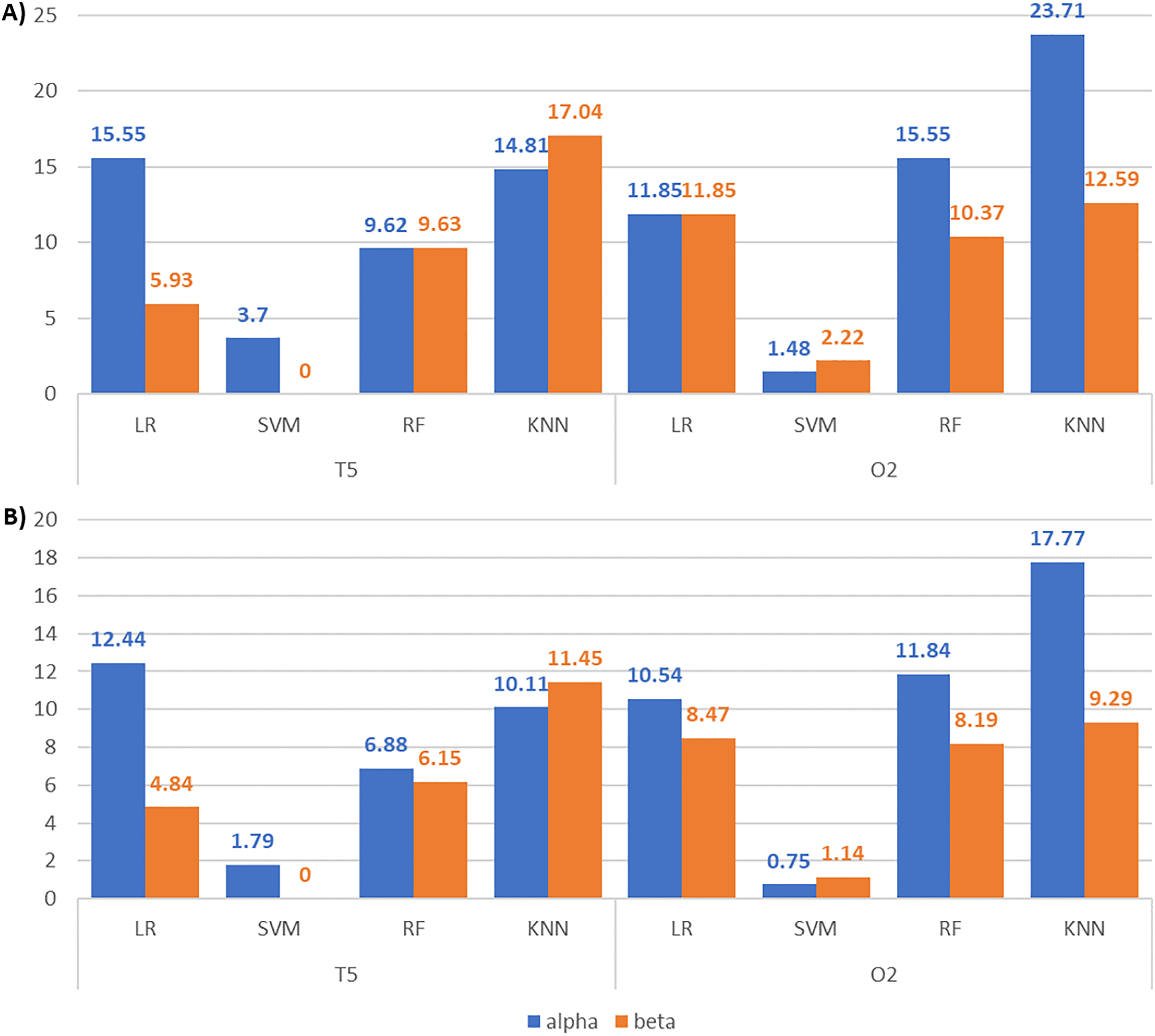
Although our enhanced BPSO performed unfavorably in distinguishing beta-band EEG signals under different auditory conditions during a light task than its alpha band counterpart, it is still worthwhile to explore the features selected by our BPSO for beta signals from T5 and O2 channels. We explored such feature selection results in multiple binary heatmaps shown in Fig. 11. Similar to Experiment I, most of the persistence statistics features are not selected (see f23–f62 in Figs. 11C, 11D, 11E, 11F and 11G), except in T5 classification with LR and RF, and O2 classification with LR. This may suggest that our enhanced BPSO performs the feature selection consistently across different bands of EEG signals.
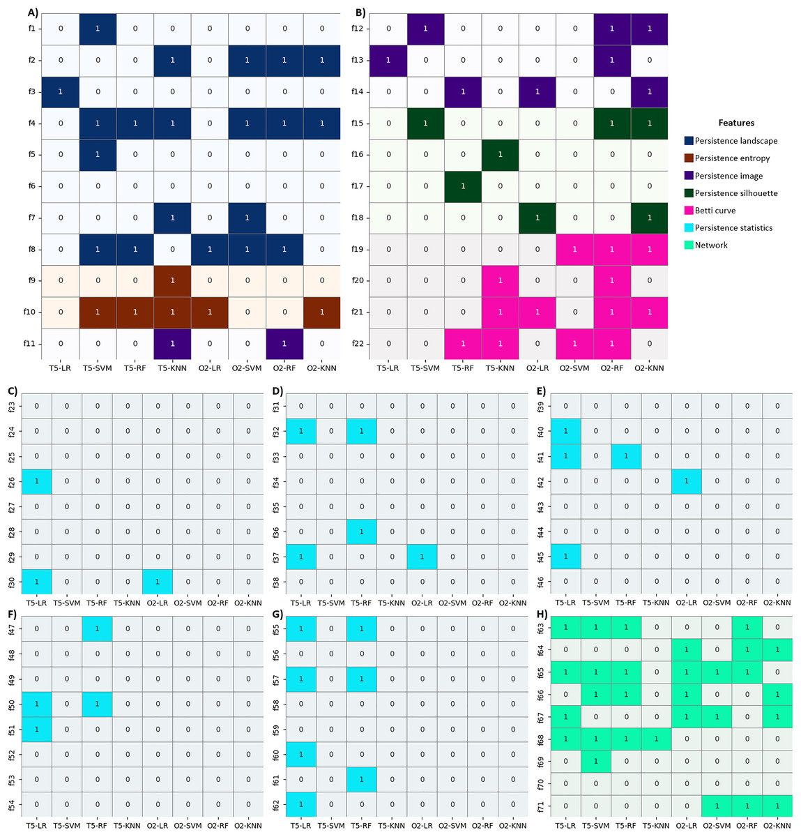
Figure 11: Heatmaps visualizing the selection of optimal features by our enhanced BPSO in each beta-band EEG signals classification.
(A and B) The selection of PH representations, (C–G ) persistence statistics, and (H) network features.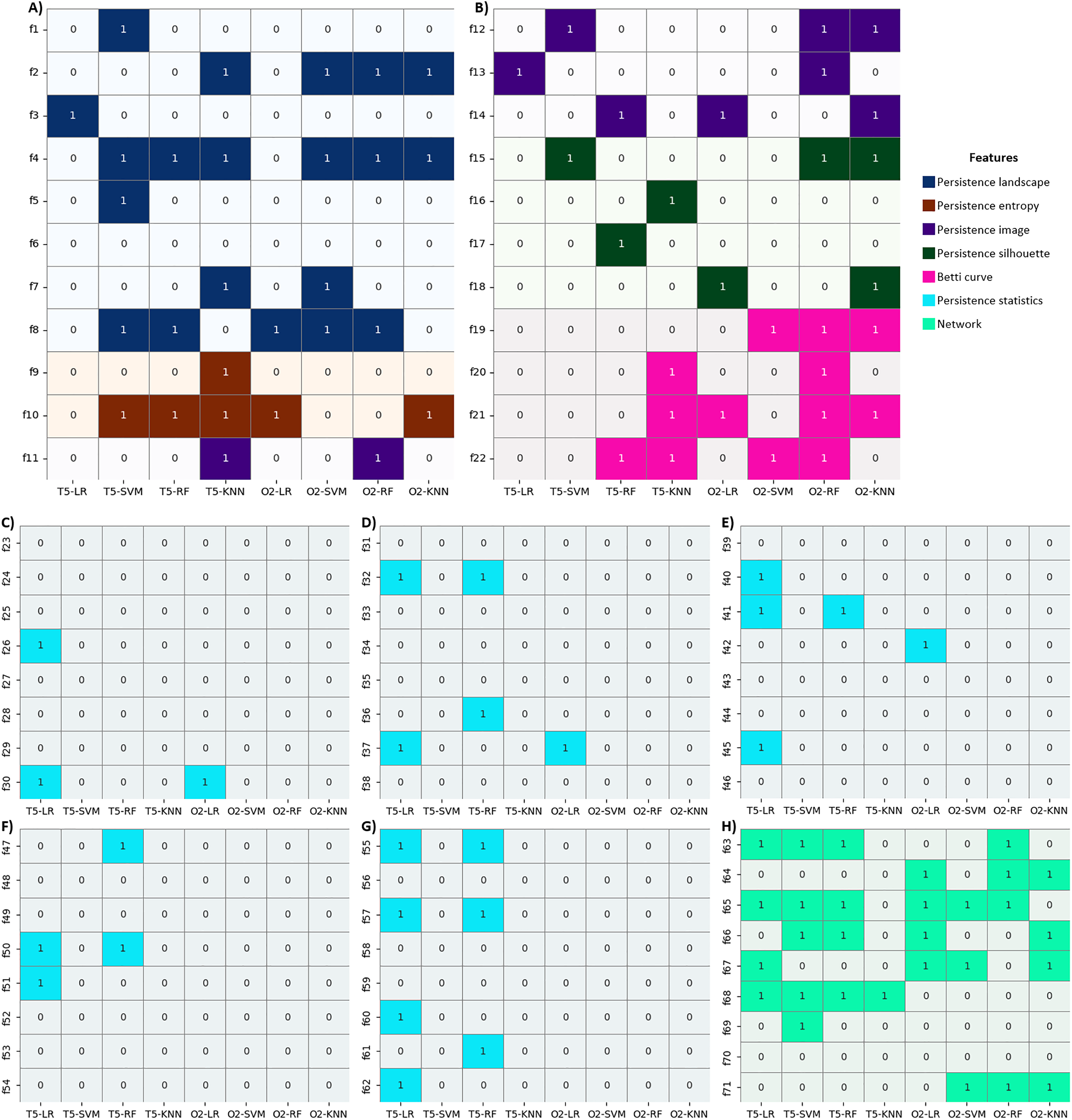
The multiple binary heatmaps also reveal that a certain number of PH representations and network features are consistently being selected, as depicted in Figs. 11A, 11B, and 11G. These results indicate that regardless of the EEG frequency and channel, the PH representations and network features always have a higher selection rate by our enhanced BPSO. However, the L2 norm of the H0 average landscape (see f6 in Fig. 11A) and the average clustering coefficient (see f70 in Fig. 11G) are excluded in all cases. The H0 landscape feature appears less informative for distinguishing beta signals, while the average clustering coefficient is omitted due to its focus on local connectivity, as observed in our Experiment II.
Comparative analysis with Bonn EEG
To demonstrate the validity of our proposed methodologies, we conducted a comparative analysis using the Bonn dataset. We conducted three classification tasks: one separating healthy from epileptic EEG signals (Z–S), and two distinguishing seizure signals from non-seizure signals recorded in different brain regions (N–S and F–S) of epileptic patients. Table 13 shows the results of each task. We observed that the LR and SVM classifiers achieved 100% accuracy and F1-score in every classification task. RF and KNN classifiers also exhibit their robustness by achieving accuracy and F1-score levels close to or exceeding 99% in all classifications. It suggests that our proposed methodologies allow multiple classifiers to acquire superior performance even with relatively short signal inputs.
| Tasks | Classifier | Accuracy | Precision | Recall | F1-score |
|---|---|---|---|---|---|
| Z-S | LR | 100 | 100 | 100 | 100 |
| SVM | 100 | 100 | 100 | 100 | |
| RF | 100 | 100 | 100 | 100 | |
| KNN | 99.50 | 100 | 99.05 | 99.51 | |
| N-S | LR | 100 | 100 | 100 | 100 |
| SVM | 100 | 100 | 100 | 100 | |
| RF | 99.50 | 100 | 98.95 | 99.46 | |
| KNN | 99.0 | 100 | 97.95 | 98.95 | |
| F-S | LR | 100 | 100 | 100 | 100 |
| SVM | 100 | 100 | 100 | 100 | |
| RF | 100 | 100 | 100 | 100 | |
| KNN | 99.00 | 100 | 98.10 | 99.00 |
Note:
The bold values indicate the best results in each task.
Table 14 compares the results obtained from our proposed methodologies with other studies in classifying EEG signals from the Bonn dataset. In classifying seizure-free and seizure signals recorded from epilepsy patients, our proposed methodologies achieve higher accuracy scores compared to other studies. Multiple studies, including our work, achieved 100% accuracy in distinguishing between seizure and non-seizure signals. However, those studies used a longer signal length or applied a sliding window to expand the sample size, unlike our proposed methodologies, which work well even with a small data size. This finding is important since using longer signals or employing additional preprocessing steps to achieve better classification increases computational cost.
| Author | Methodology | Accuracy | ||
|---|---|---|---|---|
| Z–S | N–S | F–S | ||
| Rajinikanth et al. (2023) | DWT1 + LBP2 + gray-level co-occurrence matrix + entropy + firefly algorithm + SoftMax | 98.50 | − | − |
| Hernández-Nava et al. (2024) | Parallel ictal-net neural network | − | − | 99.49 |
| Shankar et al. (2021) | Recurrence plot + CNN3 | 93.00 | − | 93.50 |
| Aayesha et al. (2021) | DWT + fuzzy rough nearest neighbor | − | 99.81 | 98.70 |
| Rashed-Al-Mahfuz et al. (2021) | STFT4 + CWT5 + CNN | 99.38 | 99.69 | 98.44 |
| Shekokar & Dour (2021) | 4-layer LSTM6 | 100 | 96.50 | 95.00 |
| Thuwajit et al. (2021) | EEGWaveNet | 99.89 | 98.26 | 97.29 |
| Yazid et al. (2021) | DWT + LBP transition histogram + LBPMAD7 + KNN | 99.94 | 99.88 | 99.70 |
| Yan et al. (2022) | MS-WTC8 + CNN | 100 | 99.80 | 99.80 |
| Shyu et al. (2023) | LBPMAD + entropy + LR | 100 | 99.00 | 95.00 |
| Zhen, Yue & Liu (2024) | PH + VG + RFE9 + SVM | 100 | 99.13 | 97.00 |
| This work | PH + VG + enhanced BPSO | 100 | 100 | 100 |
Note:
1DWT = Discrete wavelet transform; 2LBP = Local binary pattern; 3CNN = Convolutional neural network; 4STFT = Short time Fourier transform; 5CWT = Continuous wavelet transform; 6LSTM = Long short-term memory; 7LBPMAD = Local binary pattern mean absolute. deviation; 8MS-WTC = Mean-standard deviation of wavelet transform coefficient; 9RFE = Recursive feature elimination.
Robustness evaluation: independent runs and hyperparameters
While all reported results are based on five independent runs, we further validated the stability and generalizability of our enhanced BPSO by increasing the number of runs fourfold (i.e., to 20). Table S7 summarizes the minimum, maximum, mean, and standard deviation of the results obtained over the 20 runs for our T5 EEG classification across classifiers. The marginal deviation of the mean accuracy between the 5 and 20 runs, as well as the small standard deviation corroborates the stability and robustness of our enhanced BPSO (Zhu et al., 2025). As for the features selected over the 20 runs, Fig. S3 reveals that persistence landscape and silhouette features are constantly selected among other PH representation features, aligning with the results obtained from 5 BPSO runs (see Table 5). These findings demonstrate that increasing the number of independent runs did not significantly alter the derived conclusions, thereby supporting the robustness of the reported findings.
We then conducted a hyperparameter sensitivity analysis focusing on four distinct population sizes and maximum iterations to assess the effect of parameter optimization on our enhanced BPSO. These two parameters were chosen because their variation impacts sub-swarm sizes, dynamic magnitude of the inertia weight, and acceleration coefficients, subsequently affecting both the algorithm’s runtime and search efficiency.
Table S8 in the Supplemental Information presents the average hyperparameter sensitivity results obtained from five independent BPSO runs. We only focused on alpha T5 using LR and KNN, as SVM yielded relatively lower results while RF required a long execution time. While increasing the population size greatly extends the runtime, it only resulted in a small improvement in accuracy, particularly for LR classifier. The effect of the maximum iteration on runtime was rather irregular, though 200 iterations consistently produced the shortest execution time. Overall, our enhanced BPSO demonstrated stable performance across various population sizes and iteration limits with LR. For KNN, a larger population generally improved accuracy but incurred higher computational cost. Therefore, the use of a population size of 100 and a 200 maximum iterations throughout this study was justified, as it gives a good balance between accuracy and runtime.
Moreover, we reported the average execution times for PH and VG computations on 135 signals, as well as the average runtime of five independent BPSO searches with each classifier, using T5 and O2 EEG as examples, in Table S9 in the Supplemental Information. All computations were performed on a machine with an AMD Ryzen 7 6800H CPU (3.20 GHz), 16 GB RAM, and an NVIDIA RTX 3050 GPU. The PH and VG computation took around 18 min, while the BPSO search time ranged from 0.98 to 1.40 min for all classifiers except RF. The BPSO search time with the RF classifier exceeded 23 min due to its exhaustive decision tree strategy.
Discussion
The main findings of this study can be summarized as follows:
-
(1)
Our proposed BPSO feature selection algorithm successfully enhanced the non-medical EEG classification performance and identified the most and least discriminative features.
-
(2)
WVG outperformed other VG techniques in our EEG classification.
-
(3)
VR and sublevel set filtrations outperformed graph filtration in our EEG classification.
-
(4)
Sliding window segmentation has minimal impact on improving the classification performance.
-
(5)
Alpha-band EEG reflects the brain’s responses to environmental noises more effectively than beta-band EEG.
-
(6)
Our proposed PH pipeline with the enhanced feature selection algorithm achieved perfect classification accuracy on a publicly available medical EEG dataset.
This study evaluated the effectiveness of our proposed enhanced BPSO in eliminating irrelevant features and enhancing the EEG classification performance. In Experiment I, the accuracy increments achieved by our enhanced BPSO across different channels and classifiers were more than ten percent (except for SVM), with KNN exhibiting the top performance. This finding suggests that ensemble and distance-based classifiers such as RF and KNN are likely more compatible with topological and network features, demonstrating better distinguishing abilities (Zhao et al., 2022). While we omitted parameter optimization in this study, classifiers, particularly SVM, which is sensitive to parameter tuning (Sutanto et al., 2024), exhibited lower performance. The class imbalance within our dataset also impairs the classifiers’ performance, and we suggest performing oversampling and downsampling methods to address this issue in future work. Optimizing the classification models can also improve their performance (Yedukondalu et al., 2025).
Our enhanced BPSO is prone to selecting PH representations and network features over persistence statistics, suggesting that the former two features exhibit stronger discriminative power in our EEG classification. As different PH representations emphasize different aspects of PDs, their ability to capture the key topological and geometric information is heavily dependent on the signals under investigation (Turkes, Montufar & Otter, 2022). For non-medical EEG datasets which are typically more homogeneous, our feature selection algorithm consistently prefers persistence landscapes and silhouette, whereas persistence entropy is unfavorable. Persistence landscape and silhouette are more stable and robust to noise (Barnes, Polanco & Perea, 2021), thereby outperforming other PH features because they retain richer multiscale topological information by representing PD as a function, rather than a single scalar as in persistence entropy and statistics where much of the rich structural information is lost. Despite having a higher selection proportion (see Fig. 7) and larger feature set (i.e., 40 features (see Table 3)), persistence statistics only summarize the elementary descriptive statistics from PD. Their performance degrades as its feature richness increases with redundant information. Interestingly, H0 topological features are chosen in nearly all scenarios, indicating that connected component information is also crucial in capturing complex brain dynamics (Li et al., 2023).
A closer inspection of Table 5 reveals that the persistence silhouette (f17), Betti curve (f22), modularity (f65), and degree assortativity (f71) features are selected by the OZ, T6, O2, and O1 signals, respectively, across all classifiers. Moreover, the persistence landscape (f7) features appear in RF classifications for every EEG channel analyzed in this study. As previously discussed, persistence landscape and modularity features effectively boost classification performance. Meanwhile, the silhouette feature, which incorporates all landscape layers, effectively captures the geometric information of the EEG signals and improves EEG classification. As in the study by Kang et al. (2024), the Betti curve and persistence landscape features exhibit strong EEG classification performance as they effectively capture the global topological changes in the complex brain network. Moreover, degree assortativity, which reflects network connectivity, also demonstrates significant discriminative power in EEG classification, as in the study by Lee et al. (2024).
In comparing the performance of various VG methods, the WVG consistently achieved the highest classification accuracy. WVG’s superiority likely stems from its ability to capture both the amplitude and structural connectivity of EEG signals, which are strong markers that improve EEG discrimination (van den Brink et al., 2018). In contrast, the standard VG (NVG and HVG) emphasizes only the geometric relationships between data points, thereby discarding valuable information about signal amplitude and intensity (Mohammadpoory, Nasrolahzadeh & Amiri, 2025). While LPHVG benefits from having a looser visibility condition, its limited penetrable parameter choice remains a challenge and affects its performance. We propose an exhaustive comparison between WVG and other network representations, such as the ordinal pattern network and KNN graph, or a deeper investigation into additional WVG features in future studies.
As for different types of PH filtration, VR and sublevel set filtration performed well in our EEG classification. VR filtration with time delay embedding captures the periodicity (Ravishanker & Chen, 2021) while sublevel set filtration emphasizes the local extrema attributes (El-Yaagoubi, Chung & Ombao, 2023) of EEG signals. These results indicate that the periodicity and amplitude aspects of the EEG may be critical in signal classification (Wang et al., 2024; Gabeff et al., 2021). In contrast, graph filtration constructed from the VG’s adjacency matrix, which emphasizes solely the connectivity patterns of the EEG, may not sufficiently capture the essential global dynamics of EEG signals.
When classifying our EEG data, the sliding window technique had little impact on improving the performance. This limitation may arise from the choice of window size, where smaller windows often miss long-term transitions, while larger ones may overlook short-term variations (Sen et al., 2023). Therefore, future research should consider adaptive sliding windows or optimize window size selection to better capture relevant temporal dynamics in EEG signals. This study also revealed that the alpha EEG outperformed the beta EEG in differentiating signals across auditory conditions. Alpha EEG is strongly associated with attentional modulation, sensory inhibition (Mohammadi et al., 2025), and often shows pronounced oscillations as a response to the distraction. Consequently, alpha EEG serves as a more sensitive marker of cognitive adaptation to varying noise levels.
This study demonstrates a versatile PH machine learning pipeline that addresses the non-medical EEG classification challenge. Additionally, we assessed the pipeline’s potential across diverse EEG classification tasks through a cross-domain validation. The comparative analysis results using the medical Bonn EEG demonstrate the applicability of our proposed pipeline in both medical and non-medical EEG analysis. The Bonn EEG classification achieved higher classification scores likely because the amplitude changes and fluctuations are more noticeable in medical EEG compared to non-medical ones. Also, our non-medical EEG dataset has a higher degree of cross-subject variability. This finding corroborates the claim made by Caputi, Pidnebesna & Hlinka (2021) that TDA is more effective when tested on more homogenous data. Future research should evaluate the pipeline on larger and more varied datasets, extending beyond the 45 subjects currently studied, to further investigate its generalizability and robustness against cross-subject variability.
Despite the strong applicability of our pipeline, the high computational cost (see Table S7) undermines its real-time feasibility. Integrating various PH features improves PH-based classification performance (Kang et al., 2024) but further intensifies the computational demand. Future studies should prioritize parallel PH computation and refine the BPSO algorithm by employing techniques such as grid search, genetic algorithm, and neural networks to enhance performance and facilitate the real-time application of our methods in medical or BCI domains. Moreover, this study considered only single-channel EEG classification. We suggest extending to multichannel to investigate channel correlations and the differing responses to stimuli, while also testing the robustness of our pipeline in more complex classification tasks.
Conclusions
To improve non-medical EEG analysis, we developed a PH-based pipeline that integrates PH, VG, and BPSO methods to harness the strengths of multimodal features and robust feature selection. Moreover, we proposed several novel strategies to enhance the performance of the BPSO feature selection. The comprehensive analysis results highlighted the effectiveness of multimodal features, especially those derived from persistence landscape, silhouette, and weighted visibility graph, in enhancing EEG classification across channels and classifiers. An extensive examination of various PH filtrations and the sliding window approach revealed that VR filtration achieved the best performance, while sliding window segmentation had little impact on non-medical EEG classification. The analysis of EEG across frequency bands indicated that alpha EEG serves as a more effective cognitive biomarker than beta EEG. The evaluation using a public epileptic EEG dataset demonstrated the practicability of the proposed pipeline and PH in analyzing EEG across diverse domains. While the proposed pipeline achieves promising classification improvements, the lengthy computation of PH and BPSO search with a particular classifier remains challenging. Future research may focus on expanding single-channel EEG classification to multichannel, optimizing the models to reduce computational time, and evaluating the pipeline in greater detail.
Supplemental Information
45 Subjects 5 Channels 1 Trials Alpha.
The dataset includes alpha EEG signals from 45 subjects across five different channels, recorded under three distinct auditory conditions. Each column is an EEG signal recorded at a sample rate of 512 Hz, resulting in 512 rows. The column naming indicates which subject (S1–S45), channel (T5, T6, O1, O2, and OZ), and condition (Q, L, and H for quiet, low distraction, and high distraction, respectively) the respective signal belongs to. This dataset is used in all the code provided except the Experiment I statistical test, Experiment V Beta EEG, and the Bonn EEG classification code.
45 Subjects 5 Channels 1 Trials Beta.
The dataset includes beta EEG signals from 45 subjects across five different channels, recorded under three distinct auditory conditions. Each column is an EEG signal recorded at a sample rate of 512 Hz, resulting in 512 rows. The column naming indicates which subject (S1–S45), channel (T5, T6, O1, O2, and OZ), and condition (Q, L, and H for quiet, low distraction, and high distraction, respectively) the respective signal belongs to. This dataset is used in the Experiment V beta EEG code.
Stat test by classifier.
The dataset includes the metric score of the EEG classification with standard BPSO, enhanced BPSO, and without feature selection. Each column represents the respective metric score obtained from EEG signals across different channels for each fold of the 5-fold cross-validation classification. The column naming indicates which evaluation metric (ACC, PRE, REC, and F1 for accuracy, precision, recall, and F1-score, respectively), usage of feature selection algorithm (none, standard, and enhanced BPSO), and classifier (LR, SVM, RF, and KNN) the respective score belongs to. The row naming indicates which channel (T5, T6, O1, O2, and OZ) and fold (1–5) the respective score belongs to. This dataset is used in the Experiment I statistical test code.
Bonn data.
All the raw EEG data in each Bonn subset available in the provided link. Each column represents an EEG signal with 4,097 data points. The column naming indicates which subset (Z, O, N, F, and S) and segment (001–100) the respective signal belongs to. This dataset is used in the Bonn EEG classification code.