
A memory and update strategy-based social group optimization for unknown parameter identification of photovoltaic modules
- Published
- Accepted
- Received
- Academic Editor
- Bilal Alatas
- Subject Areas
- Algorithms and Analysis of Algorithms, Computer Education, Data Mining and Machine Learning, Optimization Theory and Computation
- Keywords
- Dynamic memory-guided strategy, Adaptive population update strategy, Photovoltaic model parameter identification
- Copyright
- © 2026 Ning et al.
- Licence
- This is an open access article distributed under the terms of the Creative Commons Attribution License, which permits unrestricted use, distribution, reproduction and adaptation in any medium and for any purpose provided that it is properly attributed. For attribution, the original author(s), title, publication source (PeerJ Computer Science) and either DOI or URL of the article must be cited.
- Cite this article
- 2026. A memory and update strategy-based social group optimization for unknown parameter identification of photovoltaic modules. PeerJ Computer Science 12:e3611 https://doi.org/10.7717/peerj-cs.3611
Abstract
With the increasingly severe environmental issues caused by fossil fuel consumption, clean energy technology represented by photovoltaics (PV) has attracted increasing research attention. However, the unknown parameter configuration of PV devices is related to conditions such as temperature and irradiance of the environment where the equipment is located, and existing methods often suffer from limited accuracy and reliability of parameter identification. To address these challenges, in this article, a Memory and Update Strategy-based Social Group Optimization (MUS-SGO) algorithm for PV parameter identification is proposed, aiming to enhance both accuracy and robustness. To strengthen local exploitation capability, a dynamic memory-guided strategy is employed. This strategy constructs a historical memory repository to store high-quality historical solutions and, together with the dynamic memory weights, guides MUS-SGO toward historical optimal regions. To maintain population diversity and accelerate convergence, an adaptive population update strategy is applied, which adaptively replaces a proportion of low-fitness individuals with new ones depending on the stage of MUS-SGO. Comparative experiments are conducted on the poly-crystalline KC200GT and mono-crystalline SM55 datasets under varying temperature and irradiance, using seven representative algorithms as baselines. The results demonstrate that MUS-SGO achieves a smaller root mean square error (RMSE) than the compared algorithms, with r2 values close to 1.0. This indicates that MUS-SGO ensures both high accuracy and strong robustness for PV parameter identification.
Introduction
Amid the global energy transition, the combined challenges of fossil fuel depletion, environmental degradation, and climate change have accelerated the development of renewable energy sources (Barış, Yanarateş & Altan, 2024). Among them, solar energy is the most abundant resource. It is clean, pollution-free, widely distributed, and practically inexhaustible, which makes it a core component of modern renewable energy systems (Houssein et al., 2021). With the growing penetration of photovoltaic (PV) systems in power grids, accurate modeling and parameter identification have become essential not only for evaluating PV module performance, but also for supporting key energy optimization tasks. These tasks include ultra-short-term power forecasting (Huang & Yang, 2023), maximum power point tracking (MPPT) (Esram & Chapman, 2007), inverter control (Yanarateş & Altan, 2025), grid-connected operational scheduling (Li et al., 2024), and long-term performance assessment of utility-scale PV plants. Moreover, accurate parameter estimation is fundamental for digital-twin PV modeling, fault detection, and degradation diagnosis (Angelova et al., 2024), which are crucial for enhancing the reliability and resilience of PV-integrated energy systems. Therefore, reliable PV parameter identification is not only critical for evaluating PV module performance, but also plays a foundational role in real-world system integration and advanced energy management.
As PV power generation is the main way to utilize solar energy, PV systems convert solar energy directly into electricity through the photoelectric effect of semiconductor materials (Farah et al., 2022). The configuration of unknown parameters in PV systems determines their operational efficiency, and these parameters are strongly affected by environmental conditions, with temperature and irradiance exerting particularly significant influence. For modeling and analyzing the parameter identification problem, PV systems are often abstracted into simplified models. Among these models, the single-diode model (SDM) (Arabshahi, Torkaman & Keyhani, 2020) and double-diode model (DDM) (Ganesh Pardhu & Kota, 2021) are the most widely adopted.
Existing parameter identification methods face multiple limitations. The key-point based methods (Chin & Salam, 2019; Wei et al., 2020) rely on characteristic assumptions (e.g., short-circuit current and open-circuit voltage). Although simple to apply, their accuracy is limited, making them unsuitable for high-precision applications. I–V curve-based methods for PV cells are broadly categorized into two classes: deterministic approaches and intelligent optimization approaches. Deterministic approaches (Ismaeel et al., 2021; Xu, Zhou & Li, 2023) require predefined model conditions and identify unknown parameters by solving equations. They converge quickly but are highly dependent on predefined conditions. Intelligent optimization approaches overcome the shortcomings of deterministic approaches (Zga et al., 2025). Therefore, many intelligent optimization algorithms have been proposed to enhance the accuracy and robustness of parameter identification. These approaches simulate natural phenomena or apply mathematical principles from different perspectives, providing diverse ways to tackle the PV model parameter identification challenge. Correspondingly, existing intelligent optimization approaches can be classified into three categories: original heuristic algorithms, improved single-algorithm, and hybrid algorithms.
The first category is inspired by natural phenomena or biological behaviors and uses unique search mechanisms for problem solving. Bastidas-Rodriguez et al. (2017) adopted the Genetic Algorithm (GA) to conduct global search in the PV parameter space. Ben Messaoud (2020) employed the Simulated Annealing (SA) Algorithm to handle measurement uncertainty in PV unknown parameter identification. Khare & Rangnekar (2013) utilized the Particle Swarm Optimization (PSO) Algorithm, leveraging inter-particle collaboration and fast solution localization for PV parameter identification. Askarzadeh & Rezazadeh (2013) applied the bee-behavior-inspired Artificial Bee Colony (ABC) Algorithm for PV parameter identification. Beşkirli & Dağ (2023) used the Tree Seed Optimization (TSO) Algorithm to identify PV parameters by simulating seed dispersal mechanisms. Belabbes et al. (2023) proposed the Snake Optimization Algorithm (SOA) for PV parameter identification based on snake mating behavior. Although these algorithms provide diverse global search capabilities, they commonly suffer from sensitivity to hyperparameters, strong dependence on initial populations, and a lack of mechanisms to utilize past search experience, often leading to premature convergence.
The second category improves the operators of existing algorithms to enhance performance. Kharchouf, Herbazi & Chahboun (2022) developed an improved differential evolution (DE) algorithm named MSDE, which uses the Lambert W function to select optimal crossover parameters and mutation factors for specific I–V characteristics to identify PV model parameters. Ru (2024) proposed a chaotic Butterfly Optimization Algorithm (BOA) named CLBOA for PV model parameter identification, which accelerates convergence by introducing a chaotic learning strategy. Izci, Ekinci & Hussien (2024) introduced an improved Prairie Dog Optimizer (PDO) named En-PDO, which integrates a random learning mechanism and a logarithmic spiral search mechanism for PV parameter identification. Li et al. (2019) devised an improved Teaching-learning-based optimization (TLBO) named ITLBO, featuring learner-level adaptive teaching strategies in the teacher phase and balanced exploration-exploitation tactics in the learner phase. Li et al. (2020b) proposed an enhanced adaptive DE named EJADE algorithm for identifying PV model parameters by introducing a cross-rate ranking mechanism. Xiong et al. (2024) proposed an improved Gaining-Sharing Knowledge-based algorithm (GSK) named MSGSK, which incorporates a proposed strategy selection mechanism and adjusted parameters for PV model parameter identification. Yu et al. (2017) presented a self-adaptive TLBO named SATLBO, allowing learners to dynamically select learning stages for parameter identification. Yu et al. (2019) introduced a performance-guided JAYA (PGJAYA) algorithm using adaptive chaotic perturbations to identify PV model parameters. Elhammoudy et al. (2025) proposed an improved dwarf mongoose optimization algorithm (DMO), named IDMO, for solving unknown parameters of PV models. While these improved algorithms achieve breakthroughs in convergence speed or accuracy for specific problems, they often struggle to completely circumvent the inherent limitations of their base algorithms. Furthermore, the introduction of complex operators frequently increases computational complexity.
The third category combines the advantageous operators of different algorithms to construct hybrid algorithms to achieve better problem solving results. Soliman et al. (2022) introduced AV-GWO by integrating GWO with African vultures optimization (AVO), enabling balanced global exploration and local development in parameter identification. Chen et al. (2018) proposed TLABC by hybridizing TLBO with ABC, which uses three hybrid teaching-based bee search stages to identify PV unknown parameters. Li et al. (2020a) proposed ATLDE by integrating differential evolution (DE) with learner ranking probabilities to enhance parameter identification accuracy for PV models. Chen et al. (2025) combined Multiple Linear Regression (MLR) with DE to propose MLR-DE, where the unknown parameters are first extracted via MLR and then further identified using DE. Chermite & Douiri (2025b) proposed DCS-NR by combining Differentiated Creative Search (DCS) with Newton-Raphson (NR). DCS employs a dual-strategy mechanism to ensure a comprehensive search of solutions, while NR further optimizes the parameters obtained from DCS, thereby improving the accuracy of parameter identification. Ekinci, Izci & Hussien (2024) proposed the Gazelle-Nelder-Mead (GOANM) algorithm, which synergistically integrates the Gazelle Optimization Algorithm (GOA) and the Nelder-Mead (NM) algorithm to identify unknown parameters in PV models. Wang et al. (2024) proposed a hybrid algorithm combining Imperialist Competition (ICA) and Particle Swarm Optimization (PSO), namely ICA-PSO, for effectively identifying PV models parameters. The position update strategy in ICA is replaced by the group position update strategy in PSO. Chermite & Douiri (2025a) proposed the MDE-NR algorithm, which combines the advantages of Mean Differential Evolution (MDE) and the Newton-Raphson (NR) method, thereby improving the accuracy of parameter extraction. Although these hybrid methods successfully integrate the strengths of constituent algorithms and generally show improved performance, they inevitably lead to increased algorithmic complexity and a proliferation of tunable parameters.
The above demonstrates that, despite substantial progress, existing metaheuristic methods for PV parameter identification still face several common challenges. Algorithms in the three categories either rely heavily on manually tuned hyperparameters and are prone to premature convergence, or introduce sophisticated hybrid structures that increase algorithmic complexity and the number of tunable parameters. In particular, it remains difficult to maintain sufficient population diversity while achieving a good balance between global exploration and local exploitation throughout the search process.
Therefore, we propose Memory and Update Strategy-based Social Group Optimization (MUS-SGO) for PV parameter identification, incorporating a dynamic memory-guided strategy and an adaptive population update strategy. These strategies enable MUS-SGO to exploit historical high-quality information, guide the search toward potentially optimal regions, maintain population diversity, and effectively improve both local exploitation and global exploration capabilities. To verify its accuracy and robustness in this scenario, we selected two PV modules widely used in practical applications, namely poly-crystalline KC200GT (Diab et al., 2020) and mono-crystalline SM55 (Chaibi et al., 2019), as test objects and conducted experimental comparisons between MUS-SGO and seven comparison algorithms.
The main contributions of this article are summarized as follows:
1. An improved acquiring phase based on a dynamic memory-guided strategy is proposed, in which historical best solutions are stored and dynamically weighted to guide the search towards high-quality regions, thereby enhancing the local exploitation capability of MUS-SGO.
2. An adaptive population update strategy is designed, in which low-fitness individuals are adaptively eliminated and replaced with newly generated individuals in different proportions at different stages of MUS-SGO. This mechanism dynamically maintains population diversity and improves the balance between global exploration and local exploitation.
3. An ablation experiment is conducted on the CEC17 benchmark suite to verify the independent and synergistic effects of the dynamic memory-guided strategy and adaptive population update strategy. Furthermore, MUS-SGO is applied to identify unknown parameters of PV modules for the poly-crystalline KC200GT and mono-crystalline SM55, and its performance is compared with that of seven mainstream algorithms.
The subsequent structure of this article is as follows. ‘Related Work’ introduces the related work. ‘The Proposed Method’ details MUS-SGO. ‘Simulation Results and Analysis’ analyzes the experimental results. ‘Conclusion’ concludes the article. All parameter symbols appearing in the following sections are defined in Table 1.
| Nomenclature | |||
|---|---|---|---|
| I | Output current | Nonlinear parameter | |
| V | Output voltage | Linear parameter | |
| Photo-generated current | Upper bound | ||
| Diode reverse saturation current | Lower bound | ||
| Shunt resistance | M | Historical memory repository | |
| Series resistance | Memory capacity | ||
| Diode’s ideal factor | Dynamic memory weight | ||
| The count of series resistors | Forgetting factor | ||
| The count of shunt resistors | Best memory solution | ||
| Boltzmann constant | Current number of iterations | ||
| T | Temperature | The fixed elimination interval | |
| Q | Electron charge | Current elimination ratio | |
| Diode current | Nitial elimination ratio | ||
| Shunt resistor current | Attenuation coefficient | ||
| D | Problem dimension | Maximum count of evaluations | |
| NP | Population size | NFE | Current count of evaluations |
| Best individual | Short-circuit current | ||
| C | Self-reflection factor | G | Irradiation intensity |
Related work
Solar PV model
PV module model
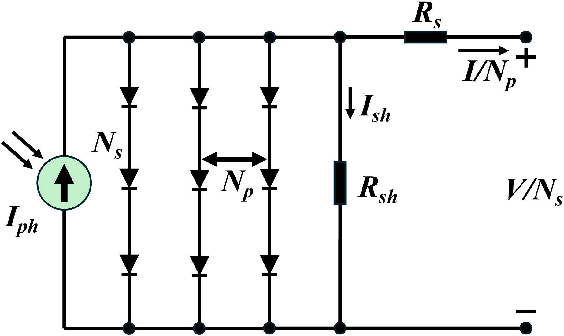
As shown in Fig. 1, the PV module model comprises several diodes configured in series and/or parallel. The output current I is formulated by Eq. (1) (Abd El-Mageed et al., 2023).
(1) where denotes the photo-generated current, represents the count of shunt resistors, indicates the diode reverse saturation current, V signifies the output voltage, refers to the series resistance, is the shunt resistance, is the diode’s ideal factor, is the count of series resistors, is the Boltzmann constant, T is the temperature, is the electron charge.
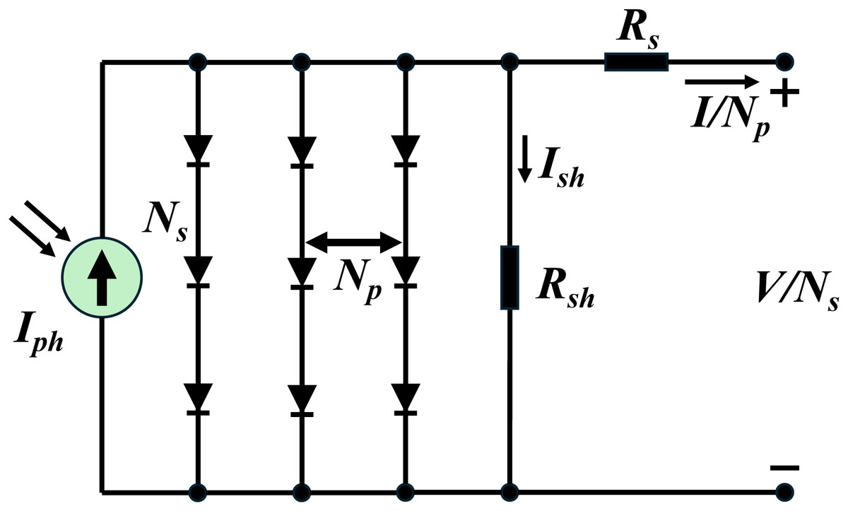
Figure 1: PV module model.
Single diode model
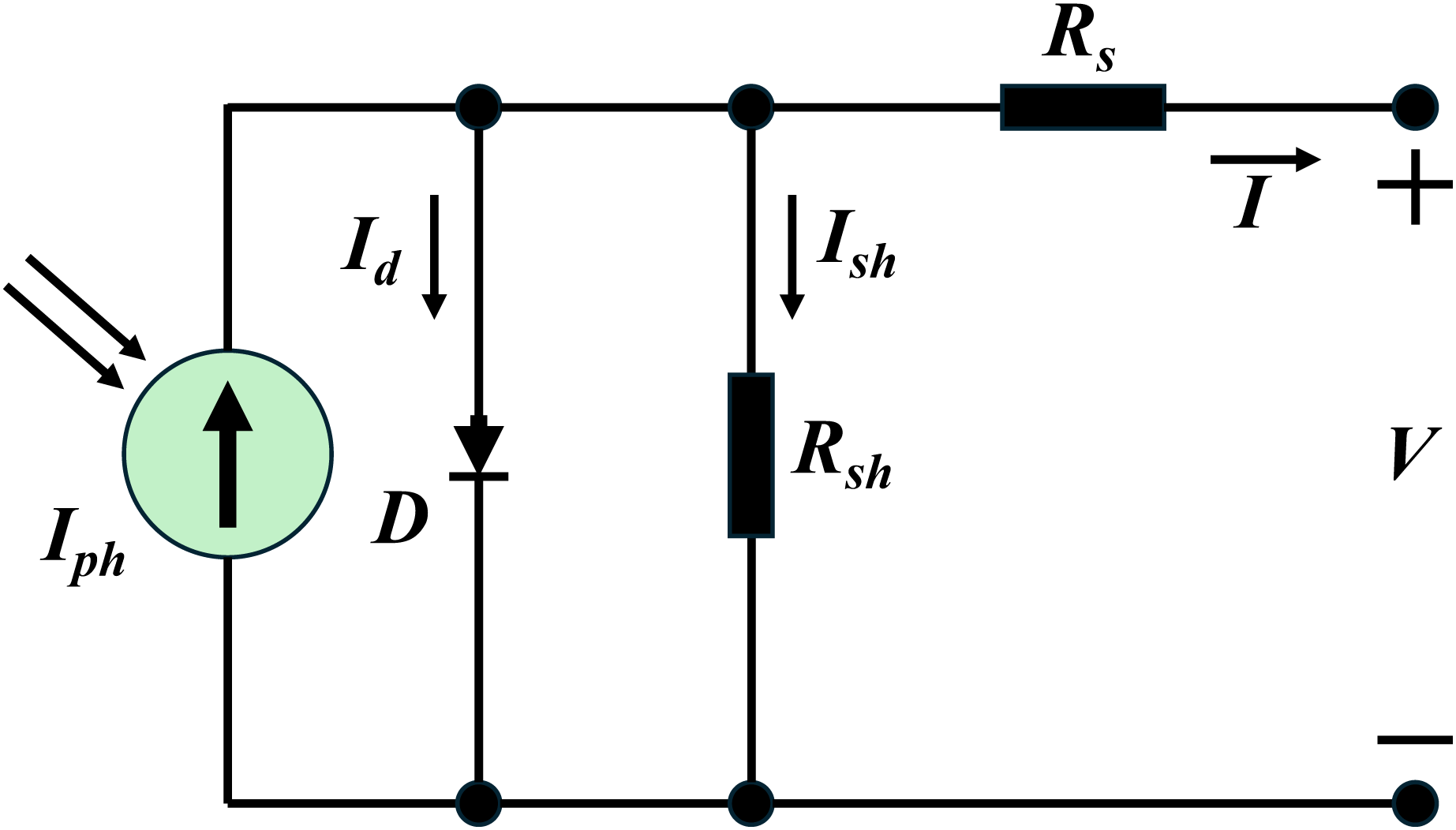
As shown in Fig. 2, when both and are set to 1 in the PV module model, the single-diode model is derived. The expression for I can be seen in Eq. (2) (Naraharisetti, Devarapalli & Bathina, 2024).
(2) where denotes the diode current, represents the shunt resistor current. Derived from Eq. (2), five unknown parameters can be identified: , , , and .
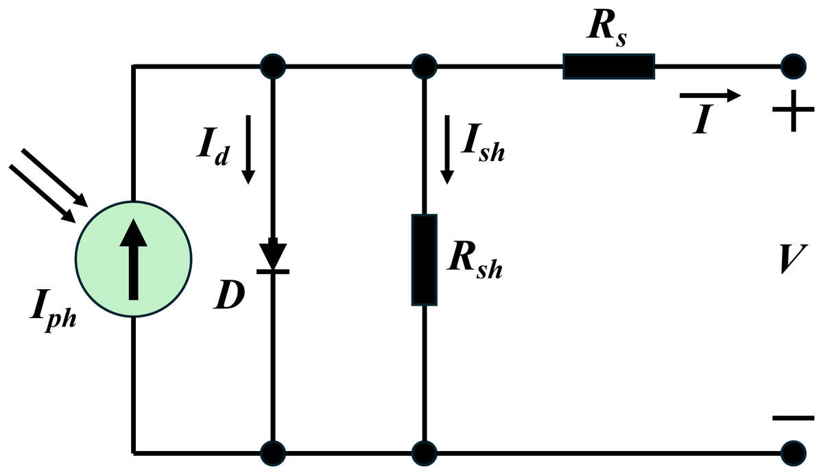
Figure 2: Single-diode model.
Optimization objective
RMSE serves as the optimization objective function, as it more effectively reflects the dispersion degree between actual data and simulated data (Abd El-Mageed et al., 2024). The definition of RMSE is given by Eq. (3).
(3) where denotes the vector of unknown parameters. L represents the amount of measured I–V data that the PV cell manufacturer supplied. is the simulated current obtained by MUS-SGO. A smaller RMSE signifies less discrepancy between simulated and measured currents, thereby indicating greater accuracy in the identification of unknown parameters.
Social group optimization
Social Group Optimization (SGO) (Satapathy & Naik, 2016) is inspired by human social behavior to solve complex problems. That is, groups are better at solving problems than individuals, and individuals can improve their own abilities through mutual influence. In SGO, each individual in the group represents a candidate solution, denoted as , where (NP is the population size) and D is the problem dimension. SGO consists of two phases: improving phase and acquiring phase.
Improving phase
In the improving phase, each individual seeks to expand their knowledge by learning from the best individual ( ) in the population. The update rule for is shown in Eq. (4).
(4)
If has a better fitness than , accept ; otherwise, keep . Where C is the self-reflection factor ( ), .
Acquiring phase
In the acquiring phase, each individual gains knowledge not only from the best individual, but also from randomly selected peers. Another individual ( ) is randomly selected, and the update rule is given by Eq. (5).
(5) where . If has a better fitness than , is accepted.
The proposed method
Motivation
SGO uses the information of the current best individual to achieve rapid convergence in the improving phase and introduces random learning among individuals in the acquiring phase to expand the search space. In addition, SGO relies on a single core parameter (C), which reduces sensitivity to parameter settings. However, it still has two critical limitations. First, individuals primarily rely on information from the current best individual and a few randomly selected individuals. As the search progresses, their positions increasingly converge, leading to a rapid loss of population diversity and a high risk of falling into local optima. Second, SGO is a “memoryless” optimization algorithm, since individual updates depend only on the current population and ignore high-quality solutions found in previous iterations. This can cause repeated exploration of already known unpromising regions and prevents the algorithm from fully exploiting high-potential regions, thereby impairing convergence speed and overall optimization performance.
Moreover, existing intelligent optimization methods also face challenges in PV parameter identification. Many original heuristic algorithms are sensitive to hyperparameters and strongly dependent on initial values. Approaches based on a single improvement mechanism often suffer from high computational cost and a persistent tendency to get trapped in local optima. Hybrid algorithms can alleviate some of these issues by combining different strategies, but they usually increase implementation complexity and introduce additional hyperparameters.
To address the above issues, MUS-SGO is designed as shown in Fig. 3. First, an unknown-parameter decomposition technique is adopted to reduce the effective problem dimension. Then, a dynamic memory-guided strategy is used to enhance local exploitation by reusing historical high-quality solutions. Finally, an adaptive population update strategy dynamically maintains population diversity throughout the search. In this way, MUS-SGO directly tackles the main shortcomings of SGO and existing algorithms, and improves both the accuracy and the robustness of PV parameter identification.
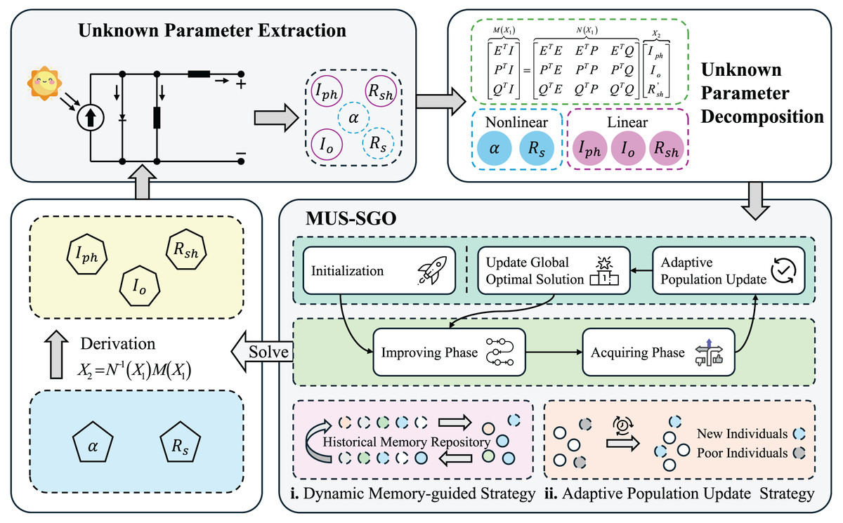
Figure 3: The structure of memory and update strategy-based social group optimization.
MUS-SGO, Memory and Update Strategy-Based Social Group Optimization; Iph, the photo-generated current; Io, the diode reverse saturation current; Rsh, the shunt resistance; Rs, the series resistance; a, the diode’s ideal factor.
Unknown parameters decomposition technique
A parameter decomposition technique is adopted to decrease the dimensionality of the problem. Equation (3) is concisely represented as shown in Eqs. (6), (7).
(6)
(7)
Building on the Benders-like decomposition method (Rahmaniani et al., 2017), the unknown parameter X can be decomposed into two sub-vectors based on linearity:
(8) where is the nonlinear sub-vector that needs to be optimized iteratively, is the linear sub-vector that can be solved directly via linear algebra once is determined. This decomposition reduces the original 5-dimensional nonlinear optimization problem to a 2-dimensional nonlinear subproblem, significantly lowering the computational complexity.
Equation (6) can be expressed in a nested form to adapt to the parameter decomposition, as shown in Eqs. (9), (10).
(9)
(10) where represents the optimization function of in relation to . The key to this decomposition is constructing a linear matrix system to solve efficiently. Since is known, can be solved by constructing a normal matrix equation in terms of and . The matrix equation is shown in Eq. (11).
(11) where E is an L-dimensional all-ones vector, P and Q are also of size L, and . The elements of vector P and Q are calculated according to Eq. (12).
(12) for . Based on Eqs. (11), (12), if is known, can be solved by , as shown in Eq. (13).
(13) where is the inverse matrix of .
Memory and update strategy-based social group optimization
Population initialization phase
In the population initialization phase, randomly generate the decision variables of each individual in the population within the domain of each dimension, as shown in Eq. (14).
(14) where and represent the upper and lower bounds, NP is the population size, D is the problem dimension, .
Generate historical memory repository
To fully utilize historical information, the historical memory repository (M) is defined as an ordered set for storing historical optimal solutions and corresponding objective function values, is shown in Eq. (15).
(15) where denotes the memory capacity and follows the general configuration rule . This rule balances two key goals. On the one hand, it allows M to accumulate sufficient historical high-quality information to guide the algorithm towards promising regions and thereby accelerate convergence. On the other hand, it avoids storing too many similar solutions, which would otherwise reduce population diversity.
The M adopts an elite replacement strategy based on the objective function value. When M is not full, newly generated solutions are directly inserted into M. Once M is full, the worst solution in M is replaced only if the new solution is better. This strategy improves the overall quality of M and strengthens the guidance provided by historical information during the search. In addition, to enable differentiated use of memory solutions, the -th solution in M is assigned a weight, and the dynamic memory weight is computed as Eq. (16).
(16) where denotes the index of the solution ( ) and is the forgetting factor (set to in this work). The factor controls the rate of weight decay, so that more recent memory solutions receive higher weights and are used more frequently. This design prioritizes recent information and enhances the ability of MUS-SGO to explore new search directions.
Improving phase
In the improving phase, each individual actively learns from the best individual ( ) in the current population based on their own current experience, thereby achieving self-improvement. The updated rule is shown in Eq. (17).
(17) where C is self-reflection factor (set to in this work), .
After completing the update, if has a better fitness than , replace , and update M according to the elite replacement strategy to accumulate high-quality search information.
Acquiring phase
In the acquiring phase, each individual performs knowledge transfer and experiential learning through multidimensional interactions. Each individual actively exchanges information with the current best individual and also randomly selects other individuals in the population to exchange knowledge. When an individual finds that another individual holds superior knowledge, it adopts this information to improve its own state. On this basis, a dynamic memory-guided strategy is introduced, which allows individuals to combine the weighted high-quality information stored in M to further correct and enhance their positions.
Randomly chosen an individual ( ) from the population, and chosen the best memory solution from M. The update rule is shown in Eq. (18).
(18) where denotes the dynamic memory weight, .
After completing the update, if outperforms , accept , and update M.
Adaptive population update strategy
To dynamically maintain population diversity and accelerate convergence, an adaptive population update strategy is introduced. This strategy uses an exponential decay mechanism to eliminate low-fitness individuals and introduce new individuals in different proportions at different stages of the algorithm. In the early stage, the strategy favors global exploration and encourages the population to explore a broad solution space. In the later stage, it gradually shifts the search toward local exploitation around already identified high-quality solutions. Population update operations are triggered when the condition in Eq. (19) is satisfied.
(19) where is the current number of iterations, is the fixed elimination interval (set to in this work). That is, the population update is performed after every 10 iterations.
During each update, the fitness of the current population individuals is sorted from highest to lowest, and the worst-performing individuals are selected for elimination. The specific number of individuals ( ) to be eliminated is dynamically controlled by an exponential decay mechanism, as shown in Eqs. (20), (21).
(20)
(21) where denotes the current elimination ratio, is the initial elimination ratio (set to ), and is the attenuation coefficient (set to ). is the maximum number of function evaluations and NFE is the current number of evaluations. The operator denotes the floor function and ensures that at least one individual is eliminated in each update. The motivation for and selection of these hyperparameters are further discussed in the “Experimental Setting” subsection.
The eliminated individuals are replaced by newly generated ones, which are produced using the same strategy as in the initialization phase. After evaluation, these new individuals are also used to update the historical memory repository M, so as to maintain the integrity and timeliness of the stored information.
Framework of MUS-SGO
Algorithm 1 presents the pseudo-code of MUS-SGO. Lines 1–3 specify the input, output and initial control parameters. Line 4 initializes the population, and line 5 evaluates the fitness of all individuals. Line 6 updates the NFE, and line 7 constructs the historical memory repository M. Line 8 starts the main loop of the algorithm, which terminates when is reached. Lines 9–15 implement the improving phase: line 10 computes a new candidate solution according to Eq. (17), and lines 11–13 compare the fitness of the new and old solutions. If the new solution outperforms the old one, the old solution is replaced and the new solution is stored in M via the elite replacement strategy. Lines 17–23 implement the acquisition phase: line 18 updates individuals according to Eq. (18), and lines 19–21 compare the fitness values of the new and old solutions. If the new solution is better, it is accepted and stored in M using the same elite replacement strategy. Lines 25–31 execute the adaptive population update strategy. Line 25 checks whether a population update should be performed based on Eq. (19); lines 26–27 rank the current population by fitness and, using Eqs. (20), (21), determine how many individuals will be eliminated; lines 28–30 randomly generate new solutions via Eq. (14) to replace the eliminated individuals and store these new solutions in M by elite replacement. Line 33 increases the iteration counter, line 34 ends the main loop, and line 35 returns the best individual in the final population.
| 1: Input: |
| 2: Output: The optimal solution |
| 3: Set , , , , , , , |
| 4: Population initialization via Eq. (14) |
| 5: Evaluate individual fitness of the population |
| 6: |
| 7: Generate history memory repository M via Eq. (15) |
| 8: while do |
| 9: for to NP do |
| 10: Calculate via Eq. (17) |
| 11: if then |
| 12: |
| 13: Update M via elite replacement |
| 14: end if |
| 15: end for |
| 16: |
| 17: for to NP do |
| 18: Calculate via Eq. (18) |
| 19: if then |
| 20: |
| 21: Update M via elite replacement |
| 22: end if |
| 23: end for |
| 24: |
| 25: if then |
| 26: Rank according to fitness |
| 27: Select eliminated individuals n via Eqs. (20), (21) |
| 28: for to n do |
| 29: Randomly generate via Eq. (14) |
| 30: Update M via elite replacement |
| 31: end for |
| 32: end if |
| 33: |
| 34: end while |
| 35: return the optimal individual in the final population |
Simulation results and analysis
Experimental setting
As mentioned earlier, the performance of MUS-SGO is tested on the poly-crystalline KC200GT and mono-crystalline SM55 PV modules. The experimental data for these two modules are obtained by extracting I–V curves under different operating conditions from the manufacturers’ datasheets, specifically covering five irradiance levels and three temperature conditions (Li et al., 2020b). Table 2 lists the parameter ranges for these two PV models, which are consistent with those used in Li et al. (2020b).
| Parameter | Poly-crystalline KC200GT | Mono-crystalline SM55 | ||
|---|---|---|---|---|
| lb | ub | lb | ub | |
| (A) | 0 | 0 | ||
| ( A) | 0 | 100 | 0 | 100 |
| ( ) | 0 | 2,000 | 0 | 2,000 |
| ( ) | 0 | 5,000 | 0 | 5,000 |
| 1 | 4 | 1 | 4 | |
In Table 2, represents the short circuit current under non-standard test conditions. at different temperature (T) and irradiation intensities (G) can be calculated by Eq. (22).
(22) where represents the short-circuit current under standard test conditions, namely and . represents the temperature coefficient under standard test conditions, and its value is referenced in Alam, Yousri & Eteiba (2015).
To validate the effectiveness of MUS-SGO, seven state-of-the-art algorithms are selected for comparative analysis, including ITLBO (Li et al., 2019), EJADE (Li et al., 2020b), SATLBO (Yu et al., 2017), PGJAYA (Yu et al., 2019), TLABC (Chen et al., 2018), ATLDE (Li et al., 2020a), and L-SHADE (Tanabe & Fukunaga, 2014). Table 3 presents the parameter configurations for all algorithms. The settings for the seven comparison algorithms are kept consistent with those reported in the corresponding literature. For MUS-SGO, the population size is fixed at to be consistent with most competing algorithms and to provide sufficient population diversity under the same . The self-reflection factor is set to , which is directly inherited from the original SGO to keep MUS-SGO close to its base algorithm. The remaining parameter settings are determined according to the design principles in ‘The Proposed Method’ and a series of preliminary experiments.
| Algorithm | Parameter setting |
|---|---|
| ITLBO | |
| SATLBO | |
| EJADE | , |
| PGJAYA | |
| TLABC | , , |
| ATLDE | , , |
| L-SHADE | , |
| MUS-SGO | , , , , , |
For the historical memory repository M, the capacity is set by the general rule , which yields when . This choice follows the common practice of using a small elite archive. If the memory is too small, the guidance from historical solutions becomes weak, whereas a too large memory tends to store many redundant, highly similar solutions and slightly reduces population diversity. The forgetting factor is fixed at , so that recently stored solutions receive higher weights while older solutions still contribute. In our preliminary tests, this weighting scheme provided a better exploration and exploitation balance than more aggressive forgetting or almost uniform weights.
In the adaptive population update strategy, the initial elimination ratio is set to , the attenuation coefficient to , and the update interval to iterations. With these values, in the early stage roughly 20–30% of the worst individuals are replaced every 10 iterations, which helps maintain diversity, while in the later stage only a few individuals are replaced, which stabilizes convergence. More aggressive settings were observed to destabilize convergence, whereas milder settings reduced the ability of MUS-SGO to escape local optima. Therefore, the above configuration is adopted as a robust compromise and is kept fixed for all PV parameter identification experiments in this article.
Additionally, all algorithms are implemented in MATLAB R2022a (The MathWorks, Natick, MA, USA). For a fair comparison, the is uniformly set to 5,000 for all algorithms. This value is chosen because preliminary experiments indicate that MUS-SGO has essentially converged by this point on the PV parameter identification problems.
Experimental results of poly-crystalline KC200GT
Results of poly-crystalline KC200GT at distinct irradiance
Table 4 presents the parameters of the poly-crystalline KC200GT identified by different algorithms at various irradiance levels when . From the parameter identification results, it can be seen that the RMSE values of MUS-SGO are 0.0014, 0.0014, 0.0012, 0.0016 and 0.0015 at irradiance levels of , , , and , respectively, which are significantly lower than those of the other algorithms. It can also be observed that increases as irradiance increases. In contrast, the remaining parameters such as and vary only slightly with changes in irradiance, indicating that these parameters are less affected by irradiance variations.
| Parameters | ITLBO | SATLBO | EJADE | PGJAYA | TLABC | ATLDE | L-SHADE | MUS-SGO |
|---|---|---|---|---|---|---|---|---|
| 1.6467 | 1.6393 | 1.6425 | 1.6424 | 1.6458 | 1.6367 | 1.6305 | 1.6461 | |
| 1.3323 | 0.2334 | 0.0165 | 0.0155 | 2.7300 | 0.4745 | 0.0652 | 0.0005 | |
| 0.1393 | 0.0476 | 0.0818 | 0.2843 | 0.2861 | 0.0564 | 0.0241 | 7.0577 | |
| 1,643.3200 | 3,056.5065 | 17.1306 | 17.0887 | 3,514.2113 | 1,263.1470 | 2,636.8764 | 12.7804 | |
| 1.5732 | 1.3943 | 1.1876 | 1.1837 | 1.6666 | 1.4618 | 1.2847 | 1.0032 | |
| RMSE | 0.0283 | 0.0168 | 0.0043 | 0.0042 | 0.0178 | 0.0202 | 0.0092 | 0.0014 |
| 3.2848 | 3.2721 | 3.2787 | 3.2784 | 3.2898 | 3.2854 | 3.2774 | 3.2878 | |
| 0.7997 | 0.2580 | 0.1148 | 0.1745 | 1.9597 | 1.2277 | 0.3906 | 0.0014 | |
| 0.0186 | 0.4009 | 2.4142 | 1.6722 | 0.0376 | 0.0195 | 0.3077 | 6.5478 | |
| 1,749.8824 | 1,826.1503 | 96.3488 | 681.3587 | 2,067.3446 | 2,054.0127 | 2,682.3477 | 13.9276 | |
| 1.4841 | 1.3797 | 1.3138 | 1.3498 | 1.5808 | 1.5282 | 1.4160 | 1.0550 | |
| RMSE | 0.0205 | 0.0178 | 0.0128 | 0.0142 | 0.0319 | 0.0251 | 0.0171 | 0.0014 |
| 4.9397 | 4.9369 | 4.9221 | 4.9344 | 4.9424 | 4.9426 | 4.9355 | 4.9343 | |
| 2.1121 | 3.7440 | 0.2283 | 0.5460 | 1.5435 | 3.9598 | 1.9826 | 0.0038 | |
| 1.9084 | 1.2703 | 3.8149 | 3.1469 | 2.1346 | 1.2111 | 1.9809 | 6.2469 | |
| 2,651.1186 | 1,888.8913 | 1,921.5912 | 3,908.8221 | 2,396.2806 | 2,266.0721 | 3,466.4117 | 13.7592 | |
| 1.5758 | 1.6392 | 1.3691 | 1.4435 | 1.5418 | 1.6455 | 1.5689 | 1.1040 | |
| RMSE | 0.0425 | 0.0469 | 0.0250 | 0.0321 | 0.0401 | 0.0474 | 0.0414 | 0.0012 |
| 6.5798 | 6.5796 | 6.5709 | 6.5719 | 6.5800 | 6.5802 | 6.5725 | 6.5713 | |
| 2.8144 | 1.3492 | 0.2509 | 0.1113 | 2.6879 | 4.2001 | 2.4235 | 0.0009 | |
| 2.0630 | 2.9592 | 3.8425 | 4.5247 | 2.2614 | 1.7885 | 2.1931 | 6.6172 | |
| 3,715.6289 | 3,176.7681 | 218.7465 | 1,028.7441 | 1,404.8867 | 3,939.7393 | 1,191.5319 | 13.7691 | |
| 1.5908 | 1.5172 | 1.3683 | 1.3075 | 1.5868 | 1.6346 | 1.5753 | 1.0353 | |
| RMSE | 0.0622 | 0.0547 | 0.0413 | 0.0330 | 0.0612 | 0.0657 | 0.0610 | 0.0016 |
| 8.2277 | 8.2228 | 8.2194 | 8.2116 | 8.2363 | 8.2309 | 8.2356 | 8.2168 | |
| 5.0883 | 1.0560 | 0.4347 | 0.3480 | 6.5152 | 7.1231 | 2.8490 | 0.0022 | |
| 2.5001 | 3.6574 | 4.2119 | 4.2567 | 2.2961 | 2.1317 | 2.8950 | 6.3670 | |
| 2,563.6609 | 3,787.4163 | 4,650.1173 | 1,638.2862 | 4,756.9567 | 781.5795 | 4,386.5522 | 14.1379 | |
| 1.6467 | 1.4870 | 1.4095 | 1.3912 | 1.6750 | 1.6847 | 1.5834 | 1.0763 | |
| RMSE | 0.0737 | 0.0556 | 0.0461 | 0.0445 | 0.0766 | 0.0779 | 0.0674 | 0.0015 |
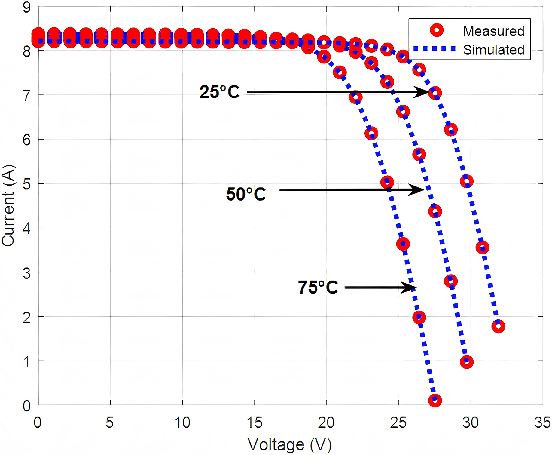
To validate the accuracy of parameter identification by MUS-SGO, the simulated current values are calculated using Eq. (1). Table 5 reports the coefficients of determination ( ) between the simulated and measured currents. As shown in Table 5, MUS-SGO achieves consistently high values. For clearer illustration, Fig. 4 depicts the fitting curves of simulated and measured currents, and it can be seen that the simulated currents obtained by MUS-SGO closely match the measured data. These results verify the high accuracy of MUS-SGO in identifying the parameters of the poly-crystalline KC200GT under varying irradiance levels.
| Irradiance | ITLBO | SATLBO | EJADE | PGJAYA | TLABC | ATLDE | L-SHADE | MUS-SGO |
|---|---|---|---|---|---|---|---|---|
| 0.9859 | 0.9950 | 0.9997 | 0.9997 | 0.9790 | 0.9928 | 0.9985 | 1.0000 | |
| 0.9985 | 0.9989 | 0.9995 | 0.9993 | 0.9965 | 0.9978 | 0.9990 | 1.0000 | |
| 0.9985 | 0.9981 | 0.9995 | 0.9992 | 0.9987 | 0.9980 | 0.9986 | 1.0000 | |
| 0.9979 | 0.9984 | 0.9993 | 0.9995 | 0.9980 | 0.9976 | 0.9980 | 1.0000 | |
| 0.9980 | 0.9989 | 0.9993 | 0.9994 | 0.9978 | 0.9977 | 0.9984 | 1.0000 |
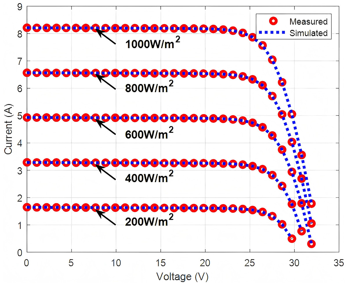
Figure 4: Measured and simulated current for poly-crystalline KC200GT obtained by MUS-SGO at distinct irradiance.
To further validate the superiority of MUS-SGO, Table 6 presents the statistical results derived from 30 independent runs, including the average (Mean), minimum (Min), maximum (Max), standard deviation (Std), and the Wilcoxon signed ranks test at a significance level of . In the Wilcoxon test, and denote the sums of positive and negative ranks, corresponding to the cases where MUS-SGO performs better or worse than its comparator, respectively; A p-value smaller than 0.05 indicates that MUS-SGO outperforms the corresponding algorithm in a statistically significant sense, which is marked with an asterisk (*).
| Algorithm | RMSE | Wilcoxon signed ranks test | ||||||
|---|---|---|---|---|---|---|---|---|
| Mean | Min | Max | Std | -value | Sig. | |||
| ITLBO | 0.0402 | 0.0283 | 0.0515 | 6.47E–03 | 465.0 | 0.0 | 1.8626E–09 | * |
| SATLBO | 0.0387 | 0.0168 | 0.0638 | 1.15E–02 | 465.0 | 0.0 | 1.8626E–09 | * |
| EJADE | 0.0060 | 0.0043 | 0.0079 | 1.07E–03 | 465.0 | 0.0 | 1.8626E–09 | * |
| PGJAYA | 0.0075 | 0.0042 | 0.0083 | 1.06E–03 | 465.0 | 0.0 | 1.8626E–09 | * |
| TLABC | 0.0427 | 0.0346 | 0.0568 | 5.44E–03 | 465.0 | 0.0 | 1.8626E–09 | * |
| ATLDE | 0.0304 | 0.0202 | 0.0425 | 5.09E–03 | 465.0 | 0.0 | 1.8626E–09 | * |
| L-SHADE | 0.0144 | 0.0092 | 0.0209 | 2.79E–03 | 465.0 | 0.0 | 1.8626E–09 | * |
| MUS-SGO | 0.0014 | 0.0014 | 0.0014 | 4.07E–11 | – | – | – | – |
| ITLBO | 0.0473 | 0.0205 | 0.0741 | 1.29E–02 | 465.0 | 0.0 | 1.8626E–09 | * |
| SATLBO | 0.0627 | 0.0178 | 0.0962 | 2.09E–02 | 465.0 | 0.0 | 1.8626E–09 | * |
| EJADE | 0.0148 | 0.0128 | 0.0177 | 1.23E–03 | 465.0 | 0.0 | 1.8626E–09 | * |
| PGJAYA | 0.0157 | 0.0142 | 0.0177 | 1.15E–03 | 465.0 | 0.0 | 1.8626E–09 | * |
| TLABC | 0.0672 | 0.0319 | 0.0867 | 1.34E–02 | 465.0 | 0.0 | 1.8626E–09 | * |
| ATLDE | 0.0416 | 0.0251 | 0.0532 | 7.39E–03 | 465.0 | 0.0 | 1.8626E–09 | * |
| L-SHADE | 0.0205 | 0.0171 | 0.0294 | 3.34E–03 | 465.0 | 0.0 | 1.8626E–09 | * |
| MUS-SGO | 0.0014 | 0.0014 | 0.0014 | 9.53E–10 | – | – | – | – |
| ITLBO | 0.0561 | 0.0425 | 0.0722 | 5.44E–03 | 465.0 | 0.0 | 1.8626E–09 | * |
| SATLBO | 0.0679 | 0.0469 | 0.1160 | 1.55E–02 | 465.0 | 0.0 | 1.8626E–09 | * |
| EJADE | 0.0313 | 0.0250 | 0.0352 | 2.93E–03 | 465.0 | 0.0 | 1.8626E–09 | * |
| PGJAYA | 0.0404 | 0.0321 | 0.0494 | 5.31E–03 | 465.0 | 0.0 | 1.8626E–09 | * |
| TLABC | 0.0668 | 0.0401 | 0.0939 | 1.27E–02 | 465.0 | 0.0 | 1.8626E–09 | * |
| ATLDE | 0.0539 | 0.0474 | 0.0687 | 4.16E–03 | 465.0 | 0.0 | 1.8626E–09 | * |
| L-SHADE | 0.0474 | 0.0414 | 0.0529 | 3.12E–03 | 465.0 | 0.0 | 1.8626E–09 | * |
| MUS-SGO | 0.0012 | 0.0012 | 0.0012 | 3.35E–08 | – | – | – | – |
| ITLBO | 0.0734 | 0.0622 | 0.0851 | 5.97E–03 | 465.0 | 0.0 | 1.8626E–09 | * |
| SATLBO | 0.0804 | 0.0547 | 0.1171 | 1.56E–02 | 465.0 | 0.0 | 1.8626E–09 | * |
| EJADE | 0.0490 | 0.0413 | 0.0570 | 3.68E–03 | 465.0 | 0.0 | 1.8626E–09 | * |
| PGJAYA | 0.0560 | 0.0330 | 0.0792 | 1.05E–02 | 465.0 | 0.0 | 1.8626E–09 | * |
| TLABC | 0.0819 | 0.0612 | 0.1002 | 8.09E–03 | 465.0 | 0.0 | 1.8626E–09 | * |
| ATLDE | 0.0745 | 0.0657 | 0.0796 | 3.81E–03 | 465.0 | 0.0 | 1.8626E–09 | * |
| L-SHADE | 0.0674 | 0.0610 | 0.0770 | 3.72E–03 | 465.0 | 0.0 | 1.8626E–09 | * |
| MUS-SGO | 0.0016 | 0.0016 | 0.0016 | 4.00E–07 | – | – | – | – |
| ITLBO | 0.0866 | 0.0737 | 0.1000 | 6.06E–03 | 465.0 | 0.0 | 1.8626E–09 | * |
| SATLBO | 0.0832 | 0.0556 | 0.1119 | 1.30E–02 | 465.0 | 0.0 | 1.8626E–09 | * |
| EJADE | 0.0552 | 0.0461 | 0.0627 | 4.25E–03 | 465.0 | 0.0 | 1.8626E–09 | * |
| PGJAYA | 0.0622 | 0.0445 | 0.0784 | 8.85E–03 | 465.0 | 0.0 | 1.8626E–09 | * |
| TLABC | 0.0937 | 0.0766 | 0.1048 | 7.20E–03 | 465.0 | 0.0 | 1.8626E–09 | * |
| ATLDE | 0.0854 | 0.0779 | 0.0933 | 4.29E–03 | 465.0 | 0.0 | 1.8626E–09 | * |
| L-SHADE | 0.0791 | 0.0674 | 0.0852 | 4.14E–03 | 465.0 | 0.0 | 1.8626E–09 | * |
| MUS-SGO | 0.0015 | 0.0015 | 0.0015 | 4.96E–06 | – | – | – | – |
Note:
A p-value smaller than 0.05 indicates that MUS-SGO outperforms the corresponding algorithm in a statistically significant sense, which is marked with an asterisk (*).
Across all tested irradiance levels, MUS-SGO consistently outperforms the other algorithms in every statistical metric. Its Mean, Min, and Max RMSE values are identical at each irradiance level, indicating exceptional stability, whereas the other algorithms exhibit markedly larger fluctuations in RMSE across all metrics. In addition, in the Wilcoxon signed-ranks test the sum of positive ranks for MUS-SGO is much larger than the sum of negative ranks , showing that its performance gains over the comparators are statistically significant. Taken together, these results confirm that MUS-SGO is superior to the competing algorithms in both accuracy and stability for identifying the parameters of the poly-crystalline KC200GT under varying irradiance.
Results of poly-crystalline KC200GT at distinct temperature
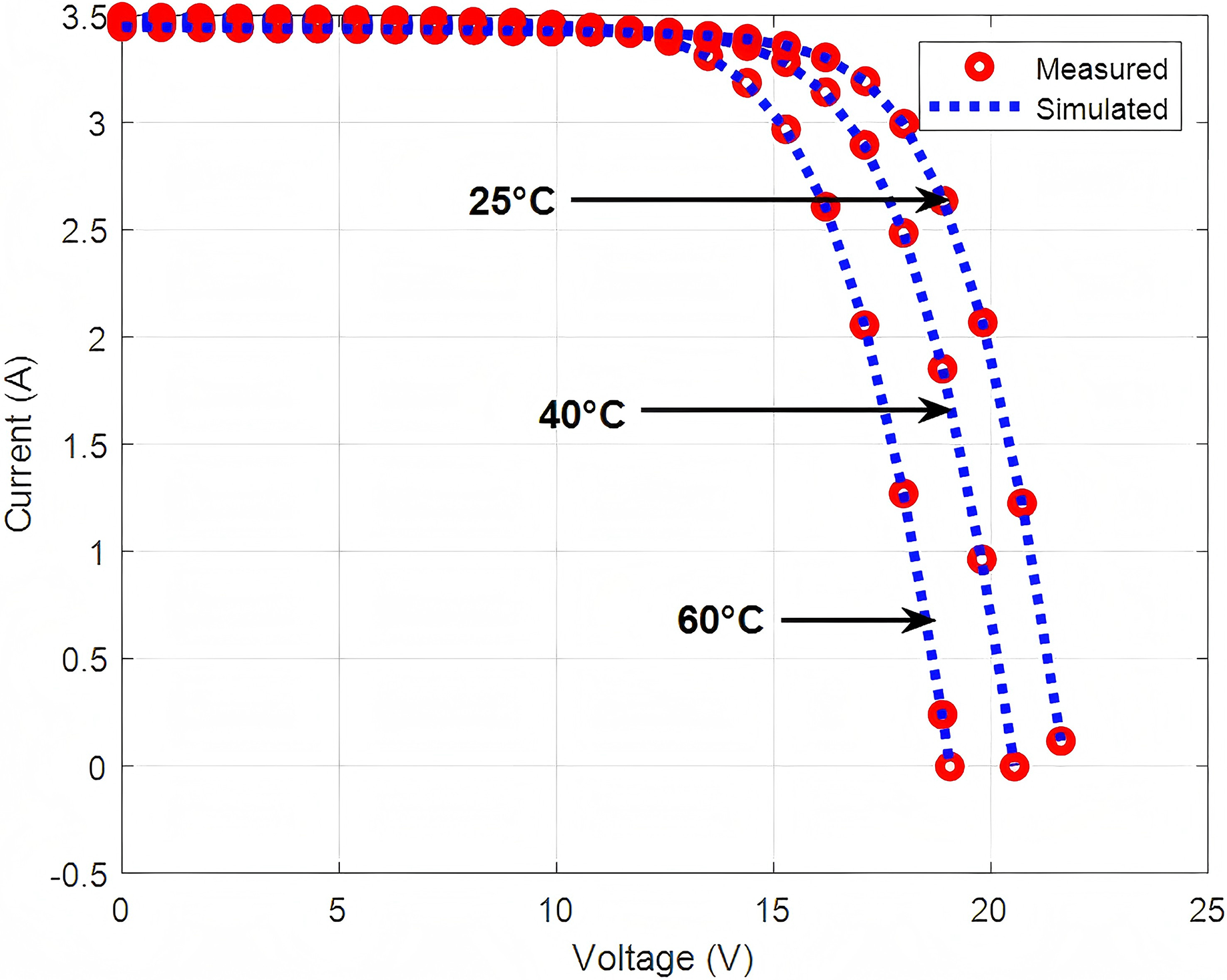
Table 7 presents the parameter identification results of different algorithms for the poly-crystalline KC200GT at varying temperatures with . At , MUS-SGO achieves the smallest RMSE of 0.0015. The RMSE values of the other algorithms are markedly higher: 0.0390 for EJADE, 0.0572 for SATLBO, 0.0701 for TLABC, 0.0418 for PGJAYA, 0.0636 for L-SHADE, and 0.0789 for ATLDE. At , MUS-SGO again attains the minimum RMSE of 0.0027. At , MUS-SGO still achieves the smallest RMSE value of 0.0044. These results indicate that, across all three temperatures, MUS-SGO consistently demonstrates superior accuracy in identifying the parameters of the polycrystalline KC200GT compared with the other algorithms.
| Parameters | ITLBO | SATLBO | EJADE | PGJAYA | TLABC | ATLDE | L-SHADE | MUS-SGO |
|---|---|---|---|---|---|---|---|---|
| 8.2228 | 8.2268 | 8.2209 | 8.2163 | 8.2244 | 8.2411 | 8.2254 | 8.2168 | |
| 4.0753 | 1.2103 | 0.2140 | 0.2876 | 3.7348 | 7.6186 | 2.1152 | 0.0022 | |
| 2.6555 | 3.5759 | 4.5522 | 4.3653 | 2.7364 | 2.1278 | 3.0786 | 6.3668 | |
| 3,165.1921 | 2,963.7645 | 3,646.8718 | 3,712.4037 | 4,996.1691 | 1,988.7441 | 1,049.8061 | 14.1395 | |
| 1.6224 | 1.4996 | 1.3529 | 1.3757 | 1.6126 | 1.6933 | 1.5524 | 1.0764 | |
| RMSE | 0.0716 | 0.0572 | 0.0390 | 0.0418 | 0.0701 | 0.0789 | 0.0636 | 0.0015 |
| 8.3129 | 8.2997 | 8.2945 | 8.2931 | 8.3054 | 8.3131 | 8.3107 | 8.2953 | |
| 5.4619 | 2.2216 | 0.8492 | 0.8122 | 6.7555 | 9.4980 | 4.7062 | 0.1259 | |
| 4.3942 | 4.9226 | 5.4615 | 5.4041 | 4.2929 | 3.9993 | 4.4760 | 6.2157 | |
| 3,999.0022 | 1,602.6910 | 3,080.9778 | 1,461.8804 | 4,211.7329 | 4,273.5421 | 2,268.4008 | 17.6698 | |
| 1.4099 | 1.3270 | 1.2487 | 1.2449 | 1.4313 | 1.4661 | 1.3952 | 1.1173 | |
| RMSE | 0.0501 | 0.0364 | 0.0231 | 0.0227 | 0.0537 | 0.0586 | 0.0477 | 0.0027 |
| 8.3763 | 8.3714 | 8.3668 | 8.3642 | 8.3876 | 8.3838 | 8.3803 | 8.3776 | |
| 6.2361 | 6.1181 | 3.3511 | 2.0275 | 8.3315 | 10.9446 | 9.2441 | 1.6311 | |
| 5.7597 | 5.7540 | 6.0343 | 6.2790 | 5.6573 | 5.4622 | 5.5438 | 6.3424 | |
| 2,163.1969 | 2,108.9805 | 3,524.3750 | 3,557.8243 | 2,993.8655 | 1,122.8408 | 1,193.9999 | 14.6386 | |
| 1.2056 | 1.2039 | 1.1549 | 1.1170 | 1.2308 | 1.2554 | 1.2400 | 1.1014 | |
| RMSE | 0.0220 | 0.0218 | 0.0115 | 0.0065 | 0.0286 | 0.0326 | 0.0296 | 0.0044 |
In addition, Table 8 reports the values of the different algorithms. At , MUS-SGO, PGJAYA, and EJADE achieve relatively high values, while at and , MUS-SGO attains the highest among all algorithms. Figure 5 depicts the fitting curves between the measured and simulated currents generated by MUS-SGO for the poly-crystalline KC200GT module at various temperatures. It can be clearly observed that the simulated currents match the measured currents very well, which further demonstrates that the parameter values identified by MUS-SGO at different temperatures are highly accurate.
| Temperature | ITLBO | SATLBO | EJADE | PGJAYA | TLABC | ATLDE | L-SHADE | MUS-SGO |
|---|---|---|---|---|---|---|---|---|
| 0.9981 | 0.9989 | 0.9995 | 0.9995 | 0.9982 | 0.9997 | 0.9986 | 1.0000 | |
| 0.9994 | 0.9997 | 0.9999 | 0.9999 | 0.9993 | 0.9992 | 0.9995 | 1.0000 | |
| 0.9999 | 0.9999 | 1.0000 | 1.0000 | 0.9999 | 0.9998 | 0.9999 | 1.0000 |
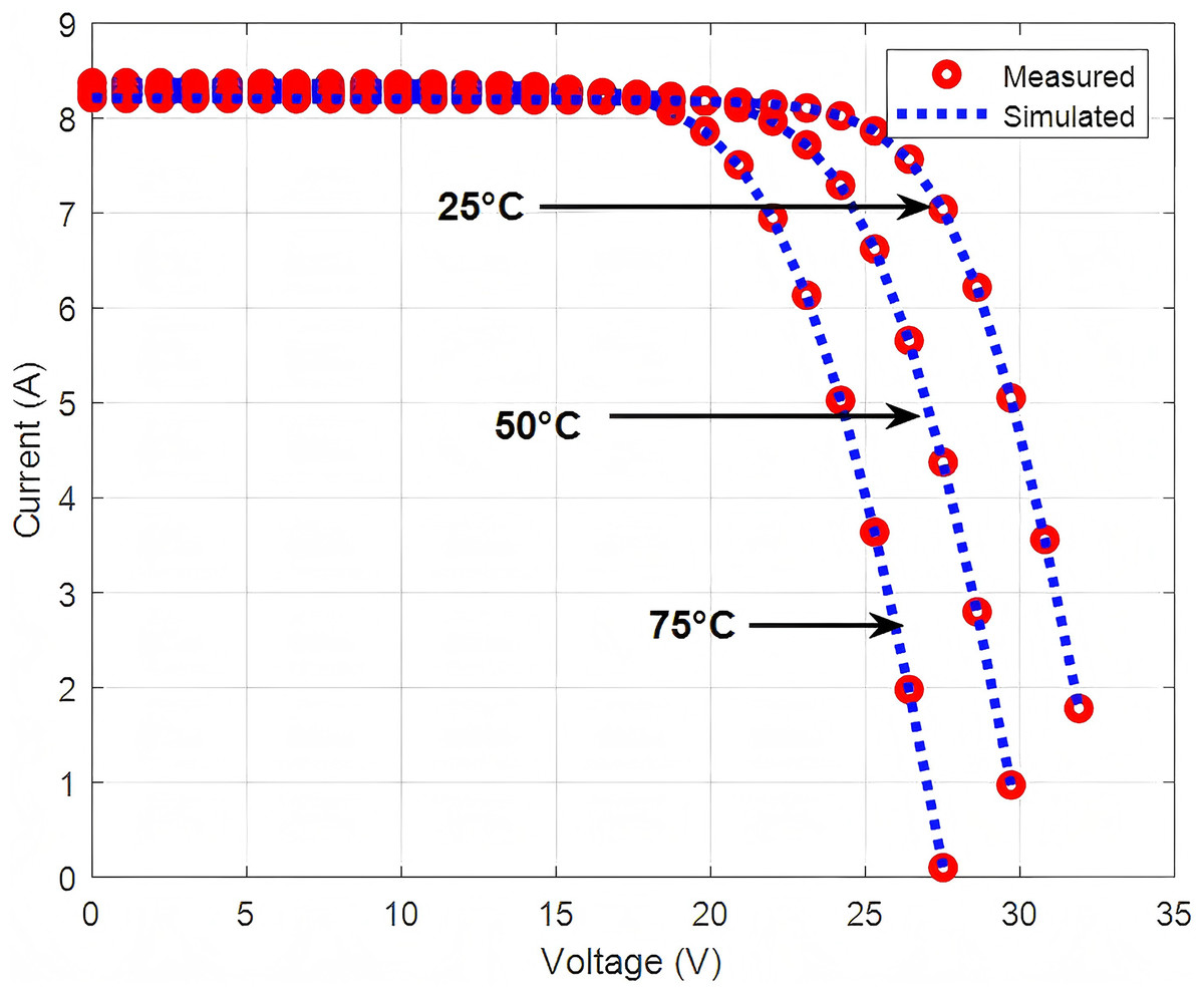
Figure 5: Measured and simulated current for poly-crystalline KC200GT obtained by MUS-SGO at distinct temperature.
Table 9 presents the statistical RMSE results of the different algorithms at various temperatures. From these metrics, MUS-SGO outperforms the other algorithms across all temperatures, and the Wilcoxon signed ranks test yields -values below 0.05 for all pairwise comparisons with MUS-SGO, indicating that its advantages are statistically significant. In contrast, the other algorithms exhibit larger variability in their RMSE values. This consistently superior performance of MUS-SGO in terms of RMSE confirms its advantage in accuracy over competing algorithms for parameter identification of the poly-crystalline KC200GT under varying temperatures.
| Algorithm | RMSE | Wilcoxon signed ranks test | ||||||
|---|---|---|---|---|---|---|---|---|
| Mean | Min | Max | Std | -value | Sig. | |||
| ITLBO | 0.0876 | 0.0716 | 0.0997 | 6.79E–03 | 465.0 | 0.0 | 1.8626E–09 | * |
| SATLBO | 0.0832 | 0.0572 | 0.1111 | 1.19E–02 | 465.0 | 0.0 | 1.8626E–09 | * |
| EJADE | 0.0538 | 0.0390 | 0.0662 | 6.64E–03 | 465.0 | 0.0 | 1.8626E–09 | * |
| PGJAYA | 0.0637 | 0.0418 | 0.0820 | 1.18E–02 | 465.0 | 0.0 | 1.8626E–09 | * |
| TLABC | 0.0913 | 0.0701 | 0.1029 | 8.67E–03 | 465.0 | 0.0 | 1.8626E–09 | * |
| ATLDE | 0.0858 | 0.0789 | 0.0906 | 3.58E–03 | 465.0 | 0.0 | 1.8626E–09 | * |
| L-SHADE | 0.0768 | 0.0636 | 0.0883 | 4.82E–03 | 465.0 | 0.0 | 1.8626E–09 | * |
| MUS-SGO | 0.0015 | 0.0015 | 0.0015 | 7.30E–07 | – | – | – | – |
| ITLBO | 0.0667 | 0.0501 | 0.0813 | 7.85E–03 | 465.0 | 0.0 | 1.8626E–09 | * |
| SATLBO | 0.0620 | 0.0364 | 0.0799 | 1.16E–02 | 465.0 | 0.0 | 1.8626E–09 | * |
| EJADE | 0.0324 | 0.0231 | 0.0534 | 5.57E–03 | 465.0 | 0.0 | 1.8626E–09 | * |
| PGJAYA | 0.0412 | 0.0227 | 0.0635 | 8.91E–03 | 465.0 | 0.0 | 1.8626E–09 | * |
| TLABC | 0.0729 | 0.0537 | 0.0898 | 8.48E–03 | 465.0 | 0.0 | 1.8626E–09 | * |
| ATLDE | 0.0713 | 0.0586 | 0.0766 | 3.83E–03 | 465.0 | 0.0 | 1.8626E–09 | * |
| L-SHADE | 0.0601 | 0.0477 | 0.0702 | 4.94E–03 | 465.0 | 0.0 | 1.8626E–09 | * |
| MUS-SGO | 0.0027 | 0.0027 | 0.0027 | 3.59E–07 | – | – | – | – |
| ITLBO | 0.0416 | 0.0220 | 0.0694 | 1.03E–02 | 465.0 | 0.0 | 1.8626E–09 | * |
| SATLBO | 0.0438 | 0.0218 | 0.0614 | 9.40E–03 | 465.0 | 0.0 | 1.8626E–09 | * |
| EJADE | 0.0170 | 0.0115 | 0.0252 | 3.97E–03 | 465.0 | 0.0 | 1.8626E–09 | * |
| PGJAYA | 0.0273 | 0.0065 | 0.0455 | 9.77E–03 | 465.0 | 0.0 | 1.8626E–09 | * |
| TLABC | 0.0539 | 0.0286 | 0.0662 | 8.77E–03 | 465.0 | 0.0 | 1.8626E–09 | * |
| ATLDE | 0.0471 | 0.0326 | 0.0603 | 5.96E–03 | 465.0 | 0.0 | 1.8626E–09 | * |
| L-SHADE | 0.0397 | 0.0296 | 0.0494 | 4.77E–03 | 465.0 | 0.0 | 1.8626E–09 | * |
| MUS-SGO | 0.0044 | 0.0044 | 0.0044 | 2.20E–06 | – | – | – | – |
Note:
A p-value smaller than 0.05 indicates that MUS-SGO outperforms the corresponding algorithm in a statistically significant sense, which is marked with an asterisk (*).
From an error-analysis perspective, the very small RMSE values and values close to 1.0 reported in Tables 4–9, together with the almost perfect overlap between the measured and simulated I–V curves in Figs. 4, 5, indicate that the residuals between measured and simulated currents are globally small and do not show a clear systematic bias along the I–V curve. In addition, by comparing the parameter estimates obtained by different algorithms in Tables 4–9, it can be observed that lower RMSE values are generally accompanied by more consistent estimates of and , whereas larger variations in have a comparatively weaker impact on the objective values. This suggests that, for the poly-crystalline KC200GT module, the overall residuals are more sensitive to and than to .
Experimental results of mono-crystalline SM55
Results of mono-crystalline SM55 at distinct irradiance
Table 10 summarizes the parameter values of the mono-crystalline SM55 identified by different algorithms at various irradiance levels when . For MUS-SGO, the corresponding RMSE values are 0.0003 at , 0.0007 at , 0.0008 at , 0.0006 at , and 0.0011 at . These results indicate that, among all compared algorithms, only MUS-SGO consistently provides the smallest RMSE across all irradiance levels.
| Parameters | ITLBO | SATLBO | EJADE | PGJAYA | TLABC | ATLDE | L-SHADE | MUS-SGO |
|---|---|---|---|---|---|---|---|---|
| 0.6784 | 0.6792 | 0.6907 | 0.6917 | 0.6798 | 0.6817 | 0.6877 | 0.6915 | |
| 2.8756 | 3.1412 | 0.3170 | 0.3154 | 4.5041 | 2.4354 | 0.8904 | 0.1464 | |
| 1.3429 | 1.2024 | 1.3375 | 2.5320 | 0.1033 | 0.2020 | 0.0511 | 7.9616 | |
| 3,398.4489 | 58.8248 | 13.0333 | 12.7737 | 112.4984 | 33.0846 | 17.0432 | 12.450 | |
| 1.7149 | 1.7315 | 1.4517 | 1.4523 | 1.7829 | 1.6955 | 1.5652 | 1.3806 | |
| RMSE | 0.0074 | 0.0168 | 0.0006 | 0.0008 | 0.0072 | 0.0056 | 0.0025 | 0.0003 |
| 1.3698 | 1.3770 | 1.3808 | 1.3781 | 1.3671 | 1.3734 | 1.3772 | 1.3828 | |
| 2.9276 | 2.3820 | 0.6407 | 1.1185 | 2.5715 | 3.0947 | 1.4453 | 0.1004 | |
| 0.1566 | 4.1228E−05 | 3.8609 | 0.7595 | 0.0857 | 0.1103 | 0.0204 | 11.0181 | |
| 91.4770 | 21.6167 | 13.9078 | 16.5080 | 2,820.3375 | 41.9843 | 17.9340 | 11.8625 | |
| 1.6949 | 1.6691 | 1.5195 | 1.5769 | 1.6761 | 1.7028 | 1.6064 | 1.3519 | |
| RMSE | 0.0066 | 0.0050 | 0.0025 | 0.0032 | 0.0072 | 0.0062 | 0.0035 | 0.0007 |
| 2.0579 | 2.0575 | 2.0654 | 2.0549 | 2.0582 | 2.0580 | 2.0631 | 2.0708 | |
| 4.0324 | 2.5710 | 1.2199 | 1.8049 | 2.9928 | 5.2285 | 2.4930 | 0.1555 | |
| 1.8418 | 3.3684 | 4.9114 | 4.3054 | 2.9642 | 0.8787 | 3.1268 | 9.1806 | |
| 796.3623 | 2,147.8343 | 22.2109 | 4,737.8121 | 133.4079 | 2,900.5100 | 36.4260 | 12.5019 | |
| 1.7263 | 1.6699 | 1.5848 | 1.6279 | 1.6888 | 1.7603 | 1.6666 | 1.3875 | |
| RMSE | 0.0089 | 0.0081 | 0.0055 | 0.0077 | 0.0082 | 0.0095 | 0.0074 | 0.0008 |
| 2.7480 | 2.7458 | 2.7518 | 2.7452 | 2.7441 | 2.7479 | 2.7473 | 2.7603 | |
| 4.6899 | 2.7647 | 1.1849 | 1.0815 | 0.8204 | 4.3568 | 3.2086 | 0.1439 | |
| 2.5135 | 3.6760 | 5.3928 | 6.1767 | 5.5623 | 2.7508 | 3.5910 | 9.3775 | |
| 2,663.0378 | 2,352.1954 | 30.1729 | 1,069.0412 | 2,982.6954 | 1,905.5102 | 414.2813 | 12.7744 | |
| 1.7343 | 1.6690 | 1.5748 | 1.5660 | 1.5336 | 1.7252 | 1.6878 | 1.3811 | |
| RMSE | 0.0103 | 0.0090 | 0.0063 | 0.0072 | 0.0114 | 0.0100 | 0.0092 | 0.0006 |
| 3.4413 | 3.4426 | 3.4436 | 3.4389 | 3.4398 | 3.4478 | 3.4435 | 3.4501 | |
| 4.8915 | 2.4025 | 1.0490 | 1.6798 | 8.6888 | 8.9972 | 4.4592 | 0.1711 | |
| 4.8640 | 6.1988 | 7.0931 | 6.5112 | 3.9200 | 3.9779 | 5.1562 | 9.1429 | |
| 4,644.2896 | 3,054.3020 | 32.6946 | 517.3689 | 4,184.1017 | 2,972.3228 | 1,506.7109 | 13.4417 | |
| 1.7409 | 1.6541 | 1.5633 | 1.6133 | 1.8186 | 1.8231 | 1.7293 | 1.3957 | |
| RMSE | 0.0184 | 0.0139 | 0.0095 | 0.0118 | 0.0229 | 0.0226 | 0.0177 | 0.0011 |
Table 11 reports the values of all algorithms, and Fig. 6 shows the fitting curves obtained by MUS-SGO. As seen from Table 11, MUS-SGO generally attains the highest values at all irradiance levels. In addition, Fig. 6 indicates that the simulated currents generated by MUS-SGO closely match the measured currents. These results confirm that MUS-SGO can accurately identify the parameters of the mono-crystalline SM55 under different irradiance levels.
| Irradiance | ITLBO | SATLBO | EJADE | PGJAYA | TLABC | ATLDE | L-SHADE | MUS-SGO |
|---|---|---|---|---|---|---|---|---|
| 0.9948 | 0.9957 | 1.0000 | 0.9999 | 0.9951 | 0.9970 | 0.9994 | 1.0000 | |
| 0.9990 | 0.9994 | 0.9999 | 0.9998 | 0.9988 | 0.9991 | 0.9997 | 1.0000 | |
| 0.9995 | 0.9996 | 0.9998 | 0.9996 | 0.9996 | 0.9994 | 0.9997 | 1.0000 | |
| 0.9995 | 0.9996 | 0.9998 | 0.9998 | 0.9995 | 0.9995 | 0.9996 | 1.0000 | |
| 0.9996 | 0.9997 | 0.9999 | 0.9998 | 0.9993 | 0.9993 | 0.9996 | 1.0000 |
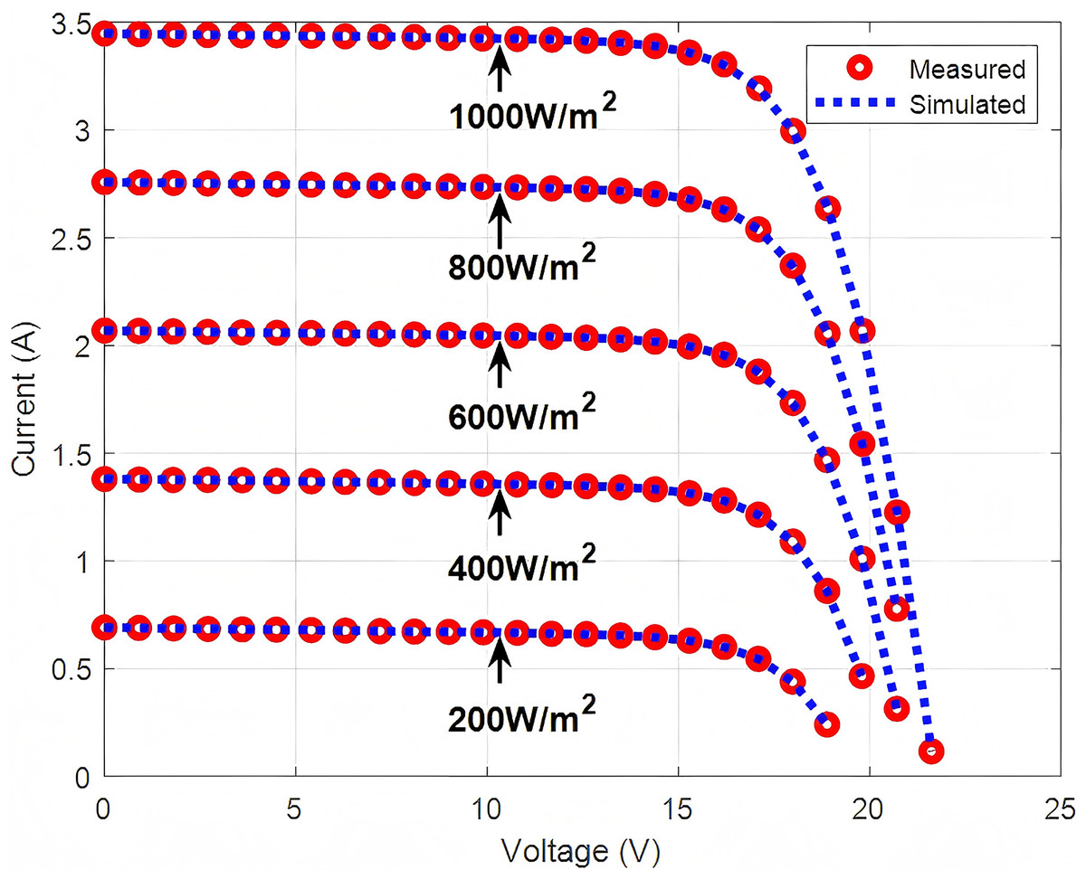
Figure 6: Measured and simulated current for mono-crystalline SM55 obtained by MUS-SGO at distinct irradiance.
The statistical results obtained by all algorithms for the mono-crystalline SM55 at different irradiance levels are summarized in Table 12. As can be seen, MUS-SGO performs best in terms of the minimum, mean, and maximum RMSE, as well as the standard deviation. The Wilcoxon signed ranks test also rejects the null hypothesis of equal performance in favour of MUS-SGO at all irradiance levels. It is worth noting that the standard deviation of MUS-SGO is much smaller than those of the other algorithms, indicating more stable optimization performance.
| Algorithm | RMSE | Wilcoxon signed ranks test | ||||||
|---|---|---|---|---|---|---|---|---|
| Mean | Min | Max | Std | -value | Sig. | |||
| ITLBO | 0.0103 | 0.0074 | 0.0143 | 1.87E–03 | 465.0 | 0.0 | 1.8626E–09 | * |
| SATLBO | 0.0091 | 0.0068 | 0.0170 | 2.35E–03 | 465.0 | 0.0 | 1.8626E–09 | * |
| EJADE | 0.0012 | 0.0006 | 0.0024 | 5.52E–04 | 465.0 | 0.0 | 1.8626E–09 | * |
| PGJAYA | 0.0034 | 0.0008 | 0.0072 | 1.81E–03 | 465.0 | 0.0 | 1.8626E–09 | * |
| TLABC | 0.0097 | 0.0072 | 0.0132 | 1.72E–03 | 465.0 | 0.0 | 1.8626E–09 | * |
| ATLDE | 0.0075 | 0.0056 | 0.0087 | 7.24E–04 | 465.0 | 0.0 | 1.8626E–09 | * |
| L-SHADE | 0.0044 | 0.0025 | 0.0071 | 9.07E–04 | 465.0 | 0.0 | 1.8626E–09 | * |
| MUS-SGO | 0.0003 | 0.0003 | 0.0003 | 5.84E–13 | – | – | – | – |
| ITLBO | 0.0149 | 0.0066 | 0.0251 | 5.74E–03 | 465.0 | 0.0 | 1.8626E–09 | * |
| SATLBO | 0.0161 | 0.0050 | 0.0281 | 6.71E–03 | 465.0 | 0.0 | 1.8626E–09 | * |
| EJADE | 0.0031 | 0.0025 | 0.0043 | 3.83E–04 | 465.0 | 0.0 | 1.8626E–09 | * |
| PGJAYA | 0.0055 | 0.0032 | 0.0072 | 1.38E–03 | 465.0 | 0.0 | 1.8626E–09 | * |
| TLABC | 0.0139 | 0.0072 | 0.0270 | 4.97E–03 | 465.0 | 0.0 | 1.8626E–09 | * |
| ATLDE | 0.0096 | 0.0062 | 0.0132 | 1.66E–03 | 465.0 | 0.0 | 1.8626E–09 | * |
| L-SHADE | 0.0056 | 0.0035 | 0.0073 | 1.09E–03 | 465.0 | 0.0 | 1.8626E–09 | * |
| MUS-SGO | 0.0007 | 0.0007 | 0.0007 | 9.24E–12 | – | – | – | – |
| ITLBO | 0.0167 | 0.0089 | 0.0299 | 5.45E–03 | 465.0 | 0.0 | 1.8626E–09 | * |
| SATLBO | 0.0198 | 0.0081 | 0.0389 | 9.05E–03 | 465.0 | 0.0 | 1.8626E–09 | * |
| EJADE | 0.0069 | 0.0055 | 0.0080 | 7.32E–04 | 465.0 | 0.0 | 1.8626E–09 | * |
| PGJAYA | 0.0088 | 0.0077 | 0.0100 | 6.62E–04 | 465.0 | 0.0 | 1.8626E–09 | * |
| TLABC | 0.0185 | 0.0082 | 0.0281 | 4.64E–03 | 465.0 | 0.0 | 1.8626E–09 | * |
| ATLDE | 0.0109 | 0.0095 | 0.0136 | 1.13E–03 | 465.0 | 0.0 | 1.8626E–09 | * |
| L-SHADE | 0.0091 | 0.0074 | 0.0102 | 6.27E–04 | 465.0 | 0.0 | 1.8626E–09 | * |
| MUS-SGO | 0.0008 | 0.0008 | 0.0008 | 8.06E–11 | – | – | – | – |
| ITLBO | 0.0134 | 0.0103 | 0.0274 | 3.54E–03 | 465.0 | 0.0 | 1.8626E–09 | * |
| SATLBO | 0.0173 | 0.0090 | 0.0445 | 8.81E–03 | 465.0 | 0.0 | 1.8626E–09 | * |
| EJADE | 0.0075 | 0.0063 | 0.0091 | 7.12E–04 | 465.0 | 0.0 | 1.8626E–09 | * |
| PGJAYA | 0.0100 | 0.0072 | 0.0124 | 1.36E–03 | 465.0 | 0.0 | 1.8626E–09 | * |
| TLABC | 0.0207 | 0.0114 | 0.0381 | 6.91E–03 | 465.0 | 0.0 | 1.8626E–09 | * |
| ATLDE | 0.0126 | 0.0100 | 0.0195 | 1.65E–03 | 465.0 | 0.0 | 1.8626E–09 | * |
| L-SHADE | 0.0107 | 0.0092 | 0.0126 | 7.29E–04 | 465.0 | 0.0 | 1.8626E–09 | * |
| MUS-SGO | 0.0007 | 0.0007 | 0.0007 | 3.21E–10 | – | – | – | – |
| ITLBO | 0.0276 | 0.0184 | 0.0352 | 3.12E–03 | 465.0 | 0.0 | 1.8626E–09 | * |
| SATLBO | 0.0257 | 0.0139 | 0.0362 | 6.40E–03 | 465.0 | 0.0 | 1.8626E–09 | * |
| EJADE | 0.0120 | 0.0095 | 0.0164 | 1.83E–03 | 465.0 | 0.0 | 1.8626E–09 | * |
| PGJAYA | 0.0179 | 0.0118 | 0.0302 | 4.75E–03 | 465.0 | 0.0 | 1.8626E–09 | * |
| TLABC | 0.0304 | 0.0229 | 0.0369 | 3.56E–03 | 465.0 | 0.0 | 1.8626E–09 | * |
| ATLDE | 0.0267 | 0.0226 | 0.0312 | 2.49E–03 | 465.0 | 0.0 | 1.8626E–09 | * |
| L-SHADE | 0.0223 | 0.0177 | 0.0293 | 2.52E–03 | 465.0 | 0.0 | 1.8626E–09 | * |
| MUS-SGO | 0.0011 | 0.0011 | 0.0011 | 3.98E–09 | – | – | – | – |
Note:
A p-value smaller than 0.05 indicates that MUS-SGO outperforms the corresponding algorithm in a statistically significant sense, which is marked with an asterisk (*).
Results of mono-crystalline SM55 at distinct temperature
The results of different algorithms for parameter identification of the mono-crystalline SM55 at distinct temperatures under a fixed irradiation intensity of are given in Table 13. At , MUS-SGO attains the smallest RMSE of 0.0011, followed by EJADE (0.0087), PGJAYA (0.0106), SATLBO (0.0156), TLABC (0.0158), ITLBO (0.0166), L-SHADE (0.0184), and ATLDE (0.0200). At and , MUS-SGOMUS-SGO again achieves the best performance, with the same minimum RMSE of 0.0037.
| Parameters | ITLBO | SATLBO | EJADE | PGJAYA | TLABC | ATLDE | L-SHADE | MUS-SGO |
|---|---|---|---|---|---|---|---|---|
| 3.4399 | 3.4400 | 3.4383 | 3.4416 | 3.4401 | 3.4458 | 3.4442 | 3.4501 | |
| 3.8032 | 3.2568 | 0.8757 | 1.1898 | 3.2393 | 6.0642 | 4.7558 | 0.1711 | |
| 5.3275 | 5.6103 | 7.5731 | 7.1211 | 5.5129 | 4.5665 | 4.8606 | 9.1429 | |
| 2,538.2052 | 4,385.1362 | 81.4434 | 3,025.4086 | 679.8443 | 932.4296 | 3,773.4714 | 13.4415 | |
| 1.7091 | 1.6901 | 1.5451 | 1.5760 | 1.6895 | 1.7691 | 1.7367 | 1.3957 | |
| RMSE | 0.0166 | 0.0156 | 0.0087 | 0.0106 | 0.0158 | 0.0200 | 0.0184 | 0.0011 |
| 3.4600 | 3.4621 | 3.4588 | 3.4618 | 3.4637 | 3.4646 | 3.4600 | 3.4691 | |
| 6.9476 | 5.5500 | 2.7891 | 3.7863 | 14.0989 | 13.5079 | 6.3115 | 1.1451 | |
| 6.4545 | 6.8096 | 7.7181 | 7.3875 | 5.3039 | 5.3126 | 6.5206 | 8.6970 | |
| 1,515.5743 | 82.7058 | 65.7047 | 3,574.6721 | 837.7864 | 1,672.1270 | 1,619.4121 | 14.8075 | |
| 1.6115 | 1.5847 | 1.5071 | 1.5400 | 1.7029 | 1.6969 | 1.5995 | 1.4178 | |
| RMSE | 0.0117 | 0.0106 | 0.0067 | 0.0088 | 0.0171 | 0.0166 | 0.0111 | 0.0037 |
| 3.4828 | 3.4875 | 3.4897 | 3.4812 | 3.4816 | 3.4850 | 3.4845 | 3.4946 | |
| 16.1214 | 13.0963 | 9.8942 | 11.8525 | 12.1076 | 20.4273 | 15.1315 | 6.9097 | |
| 7.8085 | 8.1032 | 8.3979 | 8.2870 | 8.2522 | 7.4552 | 0.0078 | 8.8528 | |
| 678.8654 | 39.9473 | 21.6608 | 2,200.8302 | 2,645.2632 | 1,350.2222 | 93.1956 | 13.4693 | |
| 1.5011 | 1.4764 | 1.4443 | 1.4645 | 1.4669 | 1.5305 | 1.4934 | 1.4051 | |
| RMSE | 0.0068 | 0.0057 | 0.0045 | 0.0063 | 0.0063 | 0.0079 | 0.0063 | 0.0037 |
In addition, Table 14 reports the values of each algorithm at different temperatures for the mono-crystalline SM55. When , all algorithms achieve high values, and MUS-SGO still attains excellent performance at and . The fitted curves between the measured and simulated currents obtained by MUS-SGO are shown in Fig. 7. It is visually evident that the simulated currents closely match the measured currents, confirming that the parameters of the mono-crystalline SM55 determined by MUS-SGO at various temperatures are highly accurate.
| Temperature | ITLBO | SATLBO | EJADE | PGJAYA | TLABC | ATLDE | L-SHADE | MUS-SGO |
|---|---|---|---|---|---|---|---|---|
| 0.9996 | 0.9997 | 0.9999 | 0.9998 | 0.9997 | 0.9995 | 0.9996 | 1.0000 | |
| 0.9998 | 0.9999 | 0.9999 | 0.9999 | 0.9997 | 0.9997 | 0.9999 | 1.0000 | |
| 1.0000 | 1.0000 | 1.0000 | 1.0000 | 1.0000 | 1.0000 | 1.0000 | 1.0000 |
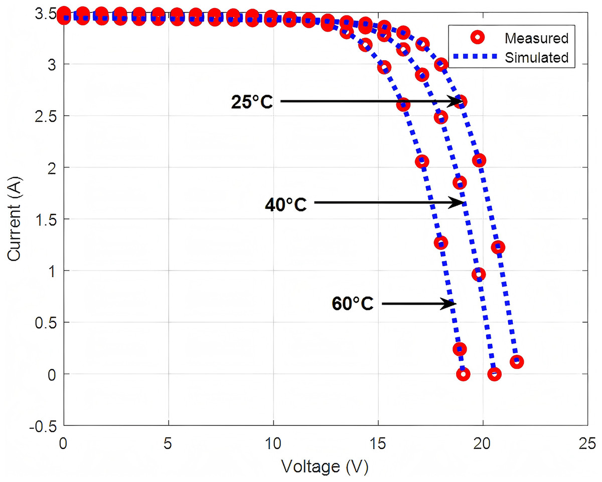
Figure 7: Measured and simulated current for mono-crystalline SM55 obtained by MUS-SGO at distinct temperature.
Table 15 displays the statistical results of all algorithms for the mono-crystalline SM55 at different temperatures. In terms of the Min, Max, and Mean RMSE values, MUS-SGO outperforms L-SHADE as well as the remaining algorithms, indicating that MUS-SGO achieves the highest identification accuracy. Moreover, the Wilcoxon signed ranks test further confirms that the performance differences between MUS-SGO and the other algorithms across all temperatures are statistically significant.
| Algorithm | RMSE | Wilcoxon signed ranks test | ||||||
|---|---|---|---|---|---|---|---|---|
| Mean | Min | Max | Std | -value | Sig. | |||
| ITLBO | 0.0269 | 0.0166 | 0.0341 | 4.24E–03 | 465.0 | 0.0 | 1.8626E–09 | * |
| SATLBO | 0.0269 | 0.0156 | 0.0449 | 7.42E–03 | 465.0 | 0.0 | 1.8626E–09 | * |
| EJADE | 0.0117 | 0.0087 | 0.0149 | 1.71E–03 | 465.0 | 0.0 | 1.8626E–09 | * |
| PGJAYA | 0.0186 | 0.0106 | 0.0268 | 4.51E–03 | 465.0 | 0.0 | 1.8626E–09 | * |
| TLABC | 0.0295 | 0.0158 | 0.0383 | 5.21E–03 | 465.0 | 0.0 | 1.8626E–09 | * |
| ATLDE | 0.0258 | 0.0200 | 0.0319 | 2.54E–03 | 465.0 | 0.0 | 1.8626E–09 | * |
| L-SHADE | 0.0221 | 0.0184 | 0.0257 | 2.05E–03 | 465.0 | 0.0 | 1.8626E–09 | * |
| MUS-SGO | 0.0011 | 0.0011 | 0.0011 | 4.95E−09 | – | – | – | – |
| ITLBO | 0.0201 | 0.0117 | 0.0274 | 3.67E–03 | 465.0 | 0.0 | 1.8626E–09 | * |
| SATLBO | 0.0172 | 0.0106 | 0.0236 | 3.26E–03 | 465.0 | 0.0 | 1.8626E–09 | * |
| EJADE | 0.0085 | 0.0067 | 0.0194 | 2.26E–03 | 465.0 | 0.0 | 1.8626E–09 | * |
| PGJAYA | 0.0120 | 0.0088 | 0.0165 | 1.87E–03 | 465.0 | 0.0 | 1.8626E–09 | * |
| TLABC | 0.0228 | 0.0171 | 0.0308 | 3.41E–03 | 465.0 | 0.0 | 1.8626E–09 | * |
| ATLDE | 0.0203 | 0.0166 | 0.0264 | 2.07E–03 | 465.0 | 0.0 | 1.8626E–09 | * |
| L-SHADE | 0.0156 | 0.0111 | 0.0212 | 2.47E–03 | 465.0 | 0.0 | 1.8626E–09 | * |
| MUS-SGO | 0.0037 | 0.0037 | 0.0037 | 6.58E−10 | – | – | – | – |
| ITLBO | 0.0109 | 0.0068 | 0.0176 | 2.65E–03 | 465.0 | 0.0 | 1.8626E–09 | * |
| SATLBO | 0.0090 | 0.0057 | 0.0131 | 2.12E–03 | 465.0 | 0.0 | 1.8626E–09 | * |
| EJADE | 0.0058 | 0.0045 | 0.0073 | 6.95E–04 | 465.0 | 0.0 | 1.8626E–09 | * |
| PGJAYA | 0.0080 | 0.0063 | 0.0122 | 1.56E–03 | 465.0 | 0.0 | 1.8626E–09 | * |
| TLABC | 0.0118 | 0.0063 | 0.0179 | 3.10E–03 | 465.0 | 0.0 | 1.8626E–09 | * |
| ATLDE | 0.0103 | 0.0079 | 0.0143 | 1.51E–03 | 465.0 | 0.0 | 1.8626E–09 | * |
| L-SHADE | 0.0087 | 0.0063 | 0.0123 | 1.37E–03 | 465.0 | 0.0 | 1.8626E–09 | * |
| MUS-SGO | 0.0037 | 0.0037 | 0.0037 | 9.23E−10 | – | – | – | – |
Note:
A p-value smaller than 0.05 indicates that MUS-SGO outperforms the corresponding algorithm in a statistically significant sense, which is marked with an asterisk (*).
Similar conclusions can be drawn for the mono-crystalline SM55. The consistently low RMSE values and high values in Tables 10–15, together with the close match between the measured and simulated I–V curves in Figs. 6, 7, show that the residuals remain small over the entire operating range. Combined with the parameter patterns observed in Tables 10–15, this indicates that, as in the poly-crystalline KC200GT, the residuals on mono-crystalline SM55 are also dominated by the accuracy of and , with playing a secondary role. The excellent fits achieved by MUS-SGO suggest that these two most sensitive parameters have been effectively identified across all irradiance and temperature conditions.
Result of convergence speed and population diversity
Result of convergence speed
To further evaluate the convergence speed of the proposed MUS-SGO and the comparative algorithms, Fig. 8 plots the RMSE and NFE curves for nine algorithms, including MUS-SGO, SGO with decomposition and seven state-of-the-art algorithms, under all operating conditions of the poly-crystalline KC200GT and mono-crystalline SM55 modules. In almost all test cases, the curve of MUS-SGO drops the fastest at the early stage and reaches the lowest RMSE within a relatively small number of function evaluations. Most of the comparison algorithms converge more slowly and level off at visibly higher RMSE values, especially under high-irradiance or high-temperature conditions, where the optimization landscape becomes more difficult. Overall, the convergence profiles indicate that MUS-SGO achieves both faster convergence speed and better final accuracy than the other advanced methods.


Figure 8: Convergence curves of different algorithms on PV models.
(A)–(E) correspond to poly-crystalline KC200GT under the condition of with irradiance , , , and ; (F)–(H) denote poly-crystalline KC200GT under with temperature , and ; (I)–(M) represent Mono-crystalline SM55 at with , 400, 600, 800, and ; (N)–(P) denote mono-crystalline SM55 under with temperature , and .
A closer inspection of Fig. 8 focuses on the comparison between MUS-SGO and “SGO with decomposition”, which augments the basic SGO with the unknown parameter decomposition technique. The “SGO with decomposition” curve usually lies below those of the seven benchmark algorithms, showing clear gains in convergence speed and final RMSE brought by the decomposition mechanism alone. However, MUS-SGO still converges faster and ends at lower RMSE levels in almost all operating conditions, and its curves are smoother and more stable, with fewer oscillations. This suggests that, on top of the benefits from parameter decomposition, the dynamic memory-guided strategy and the adaptive population update strategy further improve the balance between exploration and exploitation, leading to more reliable and efficient convergence for PV parameter identification.
Result of population diversity
To further investigate the capability of MUS-SGO to maintain population diversity during the search process, the mean pairwise Euclidean distance (MPED) (Batzelis et al., 2022) is adopted as a quantitative diversity metric. MPED measures the average Euclidean distance among all individuals in the population and thus reflects the global spread of solutions across the search space. A larger MPED indicates stronger exploration ability and a lower risk of premature convergence, whereas a rapidly diminishing MPED suggests loss of diversity and stagnation.
Figure 9 illustrates the evolution of MPED under all irradiance and temperature conditions for both the full MUS-SGO and its ablated variant without the adaptive population update strategy. Across all cases, both variants start from a similar diversity level, but the variant without the adaptive population update strategy exhibits a fast and almost monotonic decrease of MPED and quickly collapses to a very low-diversity regime. In almost all panels A–P, the red dashed curves drop sharply within the first 10–20 iterations and then remain close to zero, indicating that the search rapidly concentrates in a narrow region of the space and loses the ability to explore new areas. In contrast, MUS-SGO with the adaptive population update maintains larger MPED values for a longer period, and the blue solid curves lie consistently above the red ones over most of the optimization horizon. Particularly in panels A–E and I–M, corresponding to the standard-temperature cases, the blue curves exhibit a slower decay with several small rebounds, showing that new search directions are repeatedly injected and that the population continues to explore alternative regions instead of collapsing prematurely. Even under higher-temperature conditions (F–H and N–P), where diversity tends to vanish more rapidly, MUS-SGO still avoids the abrupt drop observed in its ablated variant and preserves a non-negligible level of MPED until later iterations. Overall, these observations confirm that MUS-SGO possesses a stronger ability to preserve population diversity throughout the search process. By maintaining a higher and more slowly decaying diversity level across a wide range of irradiance and temperature conditions, MUS-SGO effectively mitigates premature convergence and keeps the population distributed over multiple promising regions of the search space. This sustained diversity provides a more robust balance between exploration and exploitation, which is crucial for reliably identifying high-quality parameter estimates for different PV operating scenarios.


Figure 9: Population diversity curves of MUS-SGO based on Mean Pairwise Euclidean Distance (MPED) on PV model.
(A)–(E) correspond to poly-crystalline KC200GT under the condition of with irradiance , , , and ; (F)–(H) denote poly-crystalline KC200GT under with temperature , and ; (I)–(M) represent mono-crystalline SM55 at with , , , and ; (N)–(P) stand for mono-crystalline SM55 at with , and .
Ablation experiment
To validate the efficacy of the two proposed strategies in MUS-SGO, we select 12 representative functions from the CEC17 benchmark suite (Wu, Mallipeddi & Suganthan, 2017) for ablation experiments. These include one unimodal function (F1), six simple multimodal functions (F3–F8), two hybrid functions (F11–F12), and three composition functions (F22, F25–F26), which together allow a comprehensive assessment of the adaptability and optimization performance of each strategy under different landscape characteristics. The experiments are implemented in MATLAB 2022a, and the tests are conducted within the standard MTO platform (Li et al., 2023) to ensure a standardized and reproducible experimental process. To ensure fairness, all algorithms use the same parameter settings: the population size N is 100, is 500,000, and the problem dimension D is 50. This configuration is widely adopted for CEC17 problems and provides a good trade-off between solution quality and computational cost.
Four algorithmic variants are considered in this experiment: SGO, MUS-SGO1 with only the dynamic memory-guided strategy, MUS-SGO2 with only the adaptive population update strategy, and MUS-SGO with both strategies. Table 16 presents the statistical results over 30 independent runs. The results show that both MUS-SGO1 and MUS-SGO2 achieve clear performance improvements over SGO on most functions. MUS-SGO1 performs particularly well on unimodal and simple multimodal functions (F1, F3–F6), indicating that the dynamic memory-guided strategy effectively enhances local exploitation and improves early convergence ability. MUS-SGO2 obtains better results on several complex hybrid and composition functions (e.g., F11 and F25), confirming the positive role of the adaptive population update strategy in maintaining population diversity. In addition, across all test functions, the Min and Mean values of MUS-SGO are generally better than those of the other three algorithms, and its Std values are smaller, which demonstrates stronger optimization accuracy and stability.
| Function | Algorithm | Min | Max | Mean | Std |
|---|---|---|---|---|---|
| F1 | SGO | 2.4753E+08 | 8.1299E+09 | 1.9932E+09 | 1.75E+09 |
| MUS-SGO1 | 7.8377E+00 | 2.1602E+04 | 2.1198E+03 | 4.09E+03 | |
| MUS-SGO2 | 6.9196E+02 | 9.9081E+05 | 8.2415E+04 | 1.92E+05 | |
| MUS-SGO | 1.0237E+01 | 9.8313E+03 | 1.5954E+03 | 2.75E+03 | |
| F3 | SGO | 2.9946E+02 | 1.1680E+03 | 5.8707E+02 | 2.04E+02 |
| MUS-SGO1 | 1.0902E−01 | 1.7990E+02 | 8.4957E+01 | 4.31E+01 | |
| MUS-SGO2 | 3.0060E+01 | 2.9971E+02 | 1.4705E+02 | 6.63E+01 | |
| MUS-SGO | 9.0158E+00 | 2.0909E+02 | 7.5620E+01 | 4.68E+01 | |
| F4 | SGO | 1.3811E+02 | 3.0435E+02 | 2.3361E+02 | 3.55E+01 |
| MUS-SGO1 | 7.7607E+01 | 1.5123E+02 | 1.0926E+02 | 1.72E+01 | |
| MUS-SGO2 | 1.4733E+02 | 2.8556E+02 | 2.1354E+02 | 3.70E+01 | |
| MUS-SGO | 6.1687E+01 | 1.3493E+02 | 1.0110E+02 | 1.99E+01 | |
| F5 | SGO | 2.0009E+01 | 4.5575E+01 | 3.1299E+01 | 6.97E+00 |
| MUS-SGO1 | 4.7117E+00 | 1.4972E+01 | 9.3397E+00 | 2.89E+00 | |
| MUS-SGO2 | 1.2546E+01 | 3.7003E+01 | 2.7417E+01 | 5.71E+00 | |
| MUS-SGO | 6.7482E−01 | 7.7842E+00 | 3.4704E+00 | 1.80E+00 | |
| F6 | SGO | 3.3585E+02 | 7.4490E+02 | 5.2094E+02 | 9.70E+01 |
| MUS-SGO1 | 1.2678E+02 | 2.4115E+02 | 1.8679E+02 | 3.18E+01 | |
| MUS-SGO2 | 2.7822E+02 | 6.6143E+02 | 4.5636E+02 | 9.06E+01 | |
| MUS-SGO | 1.0294E+02 | 2.1608E+02 | 1.5792E+02 | 2.62E+01 | |
| F7 | SGO | 1.6727E+02 | 3.2592E+02 | 2.3374E+02 | 4.49E+01 |
| MUS-SGO1 | 8.5566E+01 | 1.3332E+02 | 1.0977e+02 | 1.28E+01 | |
| MUS-SGO2 | 1.4059E+02 | 3.0038E+02 | 2.2155E+02 | 4.28E+01 | |
| MUS-SGO | 5.6713E+01 | 1.4128E+02 | 1.0069E+02 | 2.17E+01 | |
| F8 | SGO | 2.9905E+03 | 7.8145E+03 | 4.9076E+03 | 1.44E+03 |
| MUS-SGO1 | 5.8667E+01 | 5.6800E+02 | 2.6010E+02 | 1.22E+02 | |
| MUS-SGO2 | 1.7113E+03 | 6.6992E+03 | 3.6525E+03 | 1.27E+03 | |
| MUS-SGO | 2.6507E+01 | 3.4258E+02 | 1.4049E+02 | 7.63E+01 | |
| F11 | SGO | 8.9087E+06 | 2.10786E+09 | 1.3861E+08 | 3.76E+08 |
| MUS-SGO1 | 6.7270E+04 | 5.1248E+05 | 2.1295E+05 | 1.21E+05 | |
| MUS-SGO2 | 1.9398E+05 | 2.3334E+08 | 1.0116E+07 | 4.24E+07 | |
| MUS-SGO | 5.0355E+04 | 1.5474E+06 | 5.7168E+05 | 3.14E+05 | |
| F12 | SGO | 1.0751E+04 | 2.5951E+09 | 1.5535E+08 | 5.93E+08 |
| MUS-SGO1 | 1.5979E+03 | 2.2578E+04 | 6.1852E+03 | 4.03E+03 | |
| MUS-SGO2 | 3.4822E+03 | 5.4536E+04 | 1.6949E+04 | 1.27E+04 | |
| MUS-SGO | 1.5486E+03 | 1.3468E+04 | 4.7367E+03 | 2.96E+03 | |
| F22 | SGO | 6.7697E+02 | 1.1601E+03 | 9.2174E+02 | 1.26E+02 |
| MUS-SGO1 | 5.6063E+02 | 8.2362E+02 | 6.9280E+02 | 7.26E+01 | |
| MUS-SGO2 | 7.1554E+02 | 1.1094E+03 | 8.7843E+02 | 1.21E+02 | |
| MUS-SGO | 5.3835E+02 | 7.8993E+02 | 6.2915E+02 | 4.87E+01 | |
| F25 | SGO | 3.5646E+03 | 7.5931E+03 | 5.0706E+03 | 8.88E+02 |
| MUS-SGO1 | 2.4689E+03 | 3.8796E+03 | 3.1234E+03 | 3.80E+02 | |
| MUS-SGO2 | 3.7402E+03 | 6.3116E+03 | 4.8507E+03 | 6.92E+02 | |
| MUS-SGO | 2.2122E+03 | 3.5534E+03 | 2.7709E+03 | 3.68E+02 | |
| F26 | SGO | 8.4004E+02 | 1.2540E+03 | 1.0398E+03 | 2.66E+06 |
| MUS-SGO1 | 7.1375E+02 | 1.1320E+03 | 8.4380E+02 | 1.04E+05 | |
| MUS-SGO2 | 7.0502E+02 | 1.1243E+03 | 9.0412E+02 | 3.26E+05 | |
| MUS-SGO | 5.6772E+02 | 9.6066E+02 | 7.5263E+02 | 1.87E+05 |
To further illustrate the convergence behaviour of all algorithms, Fig. 10 shows the convergence curves of SGO, MUS-SGO1, MUS-SGO2, and MUS-SGO. Overall, SGO exhibits slower convergence and poorer final accuracy on many test functions. In contrast, MUS-SGO1 converges significantly faster than SGO in the early stage of the search, while MUS-SGO2 shows a smoother convergence process in the middle and late stages. For most test functions, the convergence curves of MUS-SGO are superior to those of the other algorithms, with faster convergence and lower objective function values.


Figure 10: Ablation experiment of the MUS-SGO: convergence curve analysis on CEC17 benchmark suite.
SGO, Social Group Optimization; MUS-SGO1, SGO + the dynamic memory-guided strategy; MUS-SGO2, SGO + the adaptive population update strategy; MUS-SGO, Memory and Update Strategy-Based Social Group Optimization.
The above experiments evaluated the independent and synergistic effects of the dynamic memory-guided strategy and the adaptive population update strategy of MUS-SGO. The two strategies complement each other and produce a “ ” effect on overall performance, enabling MUS-SGO to achieve faster convergence, better solution quality, and smaller performance fluctuations, which reflects strong stability and adaptability. In summary, both improved strategies substantially enhance the performance of MUS-SGO.
Discussion
In the previous sections, the superiority of MUS-SGO has been verified by testing it on the poly-crystalline KC200GT and mono-crystalline SM55 modules under various irradiance and temperature conditions and by comparing it with seven advanced algorithms for parameter identification. These comparisons show that MUS-SGO achieves high identification accuracy and robust performance across different operating conditions. In addition, ablation experiments on the CEC17 benchmark set analyse the influence of the main components of MUS-SGO. The results show that the dynamic memory-guided strategy and the adaptive population update strategy are both effective, and that using them together gives better overall performance than using either one alone. A diversity study based on MPED further shows that MUS-SGO can maintain sufficient diversity during the search and can escape from local optima. Convergence curves comparing MUS-SGO with the other algorithms also show good convergence and lower RMSE values with more stable solutions in most cases. Although these mechanisms introduce some additional computational overhead compared with the original SGO, the clear improvements in solution quality and stability under all operating conditions indicate that MUS-SGO is very promising for parameter identification of other complex PV models.
Conclusion
This article proposes MUS-SGO to address the insufficient accuracy and reliability of PV module parameter identification under complex environmental conditions. The aim is to improve identification accuracy and robustness. The dynamic memory-guided strategy enhances local exploitation by constructing a historical memory repository for high-quality solutions and incorporating dynamic memory weights to guide searches in these areas. The adaptive population update strategy adaptively eliminates low-fitness individuals and introduces new ones proportionally, maintaining population diversity while accelerating convergence. Ablation experiments on the CEC17 benchmark suite show that both the dynamic memory-guided strategy and the adaptive population update strategy can independently improve MUS-SGO performance, and their synergistic effect yields even better results. Comparative experiments and convergence analyses on the poly-crystalline KC200GT and mono-crystalline SM55 modules under various temperature and irradiance further demonstrate that that MUS-SGO achieves higher identification accuracy and stronger robustness than other advanced algorithms.
The current validation is limited to numerical experiments on two benchmark PV modules, and the additional mechanisms in MUS-SGO introduce extra algorithmic complexity and hyperparameters. In future work, we will validate MUS-SGO using data from a wider range of PV technologies and field measurements. We also plan to explore the hybridization of MUS-SGO with deep learning-based I–V models and to embed the resulting methods into broader metaheuristic–machine-learning frameworks and adaptive PV monitoring and control systems. These directions are expected to further enhance the efficiency and applicability of MUS-SGO in complex real-world scenarios.
Supplemental Information
Current (I) and Voltage (V) Data under Different Environmental Conditions in the Poly-Crystalline KC200GT and Mono-Crystalline SM55.
Each row in the table represents the electrical characteristics of Poly-Crystalline KC200GT and Mono-Crystalline SM55 under specific environmental conditions. each data point in the V column indicates the measured voltage value of the Poly-Crystalline KC200GT under the aforementioned environmental conditions, while the corresponding value in the I column represents the associated current.
Identifying unknown parameters of photovoltaic models using MUS-SGO.
MUS-SGO code mainly includes the improving phase and the acquiring phase, and adopts a dynamic memory-guided strategy and an adaptive population update strategy.