
Real-time monitoring and optimization of SPN networks in distribution grid communication based on big data analysis
- Published
- Accepted
- Received
- Academic Editor
- Bilal Alatas
- Subject Areas
- Computer Networks and Communications, Data Mining and Machine Learning, Data Science, Optimization Theory and Computation, Internet of Things
- Keywords
- SPN network, Distribution grid communication, Real-time monitoring, Topology optimization
- Copyright
- © 2026 Wei et al.
- Licence
- This is an open access article distributed under the terms of the Creative Commons Attribution License, which permits unrestricted use, distribution, reproduction and adaptation in any medium and for any purpose provided that it is properly attributed. For attribution, the original author(s), title, publication source (PeerJ Computer Science) and either DOI or URL of the article must be cited.
- Cite this article
- 2026. Real-time monitoring and optimization of SPN networks in distribution grid communication based on big data analysis. PeerJ Computer Science 12:e3610 https://doi.org/10.7717/peerj-cs.3610
Abstract
With the rapid integration of wind and solar energy into distribution grids, the high-frequency fluctuations of renewable energy output pose significant challenges to the Software-Defined Power Communication Converged Network (SPN), particularly in terms of dynamic communication load surges and inefficient topology adaptation. This study addresses these critical issues by leveraging the State Grid Wind-Solar Competition Dataset to develop a data-driven SPN monitoring and optimization framework. Key innovations include three core components: (1) an attention-enhanced long short-term memory (LSTM) model fused with Variational Mode Decomposition (VMD) for SPN communication delay prediction, which prioritizes high-correlation features from the dataset and achieves a mean absolute error (MAE) of 8.2 ± 0.3 ms for 1-hour-ahead prediction (the predicted target is explicitly defined as SPN communication delay in milliseconds, and the communication load index Lt (in Mbps) is a key influencing feature); (2) a wind-solar fluctuation grade-driven SPN topology self-optimization method, which classifies renewable fluctuations into five grades via K-Means clustering and dynamically adjusts routing weights considering Flexible Ethernet (FlexE) hard slicing, reducing average communication latency by 62.0 ± 3.2% and packet loss rate from 5.8 ± 0.4% to 0.3 ± 0.1%; (3) a cross-climate SPN communication fingerprint library integrating seasonal features, which integrates statistical characteristics of “wind-solar features-communication load-seasonal fluctuations” from multi-climate sites, shortening new site debugging time by 97.9 ± 0.5% (from 24 to 0.5 h) and reducing post-matching latency by 26.8 ± 1.3%. Comprehensive experimental validation (10 random seed runs) demonstrates that the proposed framework effectively bridges the gap between renewable energy dynamics and power communication network operations.
Introduction
Research background
Under the dual impetus of the “dual carbon” strategy and the construction of a new power system, distribution networks are rapidly evolving from traditional unidirectional radiation structures to active distribution networks with a high proportion of distributed energy resources (DER) (Li et al., 2022; Yang et al., 2023). However, the explosive grid connection of intermittent resources such as photovoltaic and wind power has brought multiple challenges including voltage over-limit, power reverse transmission, sharp increase in line loss and reduction in operational safety margin (Wang et al., 2024; Chuang et al., 2025). To fully unleash the flexible adjustment potential of DER and ensure real-time optimized scheduling under transmission and distribution coordination, the communication network, as the “nervous system”, must provide the ability of reliable perception at the millisecond level and precise synchronization at the hundreds of microseconds level.
Facing the new characteristics of “small bandwidth, large connection, strong burst, and high reliability” of distribution Network services, Slicing Packet Network (SPN) has become the preferred choice for the new generation of communication bearer with its advantages such as Flexible Ethernet (FlexE) hard slicing, ultra-low latency, and large connection synchronization. However, there is still a lack of systematic research on its real-time operation mechanism, monitoring accuracy and optimization strategies under complex electromagnetic environments and massive data injection (Yerimah et al., 2024; Cai et al., 2019). Therefore, how to build a real-time monitoring and optimization framework for SPN networks based on big data analysis has become the primary scientific issue for achieving coordinated dispatching of transmission and distribution and enhancing the safe and economic operation of active distribution networks.
Physical mechanism of renewable fluctuation impact on SPN
To address the lack of technical explanation for how wind-PV fluctuations cause SPN packet loss and delays, this section elaborates on the core physical pathways from the perspective of power system operation logic and SPN technical characteristics, focusing on the coupling relationship between renewable energy dynamics and power communication demand.
Two core physical pathways linking renewable fluctuations to SPN performance degradation
Renewable energy (wind/PV) fluctuations affect SPN communication performance through two interrelated physical processes, both rooted in the inherent coupling between distribution grid operation and communication service demand:
-
(1)
Pathway 1: Burst of Communication Traffic Induced by Sudden Renewable Output Changes
Wind and PV power generation exhibit inherent intermittency and randomness—their output can change sharply within short time windows (e.g., a 3 m/s increase in wind speed or a 300 W/m2 drop in total solar irradiance (TSI) due to cloud shading within 15 min). Such sudden output changes trigger an immediate surge in two types of critical communication traffic in the power system:
-
a.
Real-Time Control Commands: The distributed Energy Management System (EMS) must send instantaneous control instructions to distributed energy resources (DERs) to maintain grid stability—for example, active power curtailment to avoid voltage over-limit, reactive power compensation to adjust power factor, or start-stop control of backup units. Unlike general telecom data, these control commands have strict real-time requirements (latency threshold < 50 ms) and their quantity can increase 3–5 times compared to stable operating conditions. This surge directly overloads the dedicated SPN slice allocated to control services;
-
b.
Massive Monitoring Data Upload: Smart meters, ring main unit (RMU) sensors, and wind/PV turbine controllers generate high-frequency monitoring data (voltage, current, frequency, equipment status) with a sampling interval of 1–5 s. When renewable output fluctuates sharply, the data volume increases proportionally to capture the transient state of the grid, reaching 2–3 times the average load.
SPN adopts FlexE hard slicing technology to ensure service isolation—each type of traffic (control commands, monitoring data) is assigned a fixed bandwidth slice. The sudden traffic surge exceeds the bandwidth capacity of the dedicated slice, leading to packet queuing at SPN nodes. Once the queue length exceeds the buffer capacity, packet loss occurs, and queuing delay directly accumulates to the total communication latency.
-
-
(2)
Pathway 2: Unbalanced Traffic Distribution Caused by Spatial-Temporal Randomness of Fluctuations
Wind-PV fluctuations are not spatially uniform across the distribution grid—for example, a certain region may experience severe wind power fluctuations due to local gusts, while an adjacent region remains stable. This spatial heterogeneity leads to uneven distribution of SPN link traffic:
-
a.
Overloaded Links: SPN links serving regions with severe renewable fluctuations bear traffic exceeding 70% of their rated bandwidth (the industry-recognized overload threshold). For hard slices with fixed bandwidth, overload cannot be mitigated by occupying other slices’ resources (to ensure service isolation), resulting in persistent packet loss and latency;
-
b.
Underutilized Links: Conversely, links serving regions with stable renewable output have traffic utilization below 30%, leading to wasted bandwidth resources that cannot be dynamically allocated to overloaded links in real time.
This unbalanced traffic distribution exacerbates the performance degradation of SPN—overloaded links become bottlenecks for the entire communication network, while underutilized links fail to provide redundant capacity, reducing the overall fault tolerance and stability of the system.
-
Linkage to mathematical modeling in this study
The above physical mechanisms directly inform the mathematical models designed in Chapter 2, ensuring theoretical consistency between mechanism analysis and quantitative modeling:
The “traffic burst” in Pathway 1 is quantified by the SPN communication load model (SPN Communication Load-Delay Model), where captures the linear relationship between renewable fluctuation amplitude and communication load surge; The “load-latency” coupling in both pathways is formalized by the mapping formula (mathematical formulation of the load-delay model), which quantifies how traffic surge translates to SPN communication latency; The topology optimization model (Topology Self-Optimization with Routing Weights) addresses unbalanced traffic distribution by dynamically adjusting routing weights based on fluctuation grade, FlexE slice utilization, and service priority—effectively diverting traffic from overloaded links to underutilized ones.
In order to fully leverage the low latency and high reliability carrying potential of SPN in distribution network communication, it is urgently necessary to carry out targeted optimization of its topology. SPN topology optimization aims to improve network performance (latency, reliability, throughput) via routing adjustment, bandwidth allocation, and node reconfiguration. Existing studies can be categorized into two groups: Static Topology Optimization and Dynamic Topology Optimization (Yang et al., 2026). Early research focused on static routing strategies based on fixed parameters. For example: Li et al. (2025) proposed an SDN-based routing algorithm to minimize latency by optimizing link weight assignment, achieving a 15% latency reduction in a 10-node SPN testbed. However, the algorithm ignored traffic dynamics, leading to congestion during peak loads. Azimian et al. (2022) developed a bandwidth-aware topology optimization method that maximizes link utilization, but it failed to consider the impact of renewable energy fluctuations on traffic distribution. Zhang et al. (2025) integrated reliability constraints into SPN topology design, improving fault tolerance by 20% but increasing complexity and latency. These methods are effective for stable loads but perform poorly in high-renewable-penetration grids due to their inability to adapt to dynamic traffic changes.
To solve the above problems, recent studies have begun to incorporate dynamic parameters to adjust SPN topology: Suo et al. (2023) proposed a traffic-aware routing algorithm that updates routes every 5 min based on real-time link utilization, reducing packet loss rate by 30% in a PV-rich distribution grid. However, the algorithm did not consider the root cause of traffic fluctuations (i.e., renewable energy dynamics) and relied on short-term traffic forecasting with high uncertainty. Chen et al. (2021) introduced a temperature-aware topology optimization method, as temperature affects optical fiber transmission loss. The method reduced latency by 18% but was ineffective for high-frequency fluctuations, as temperature changes on a hourly scale. Tolani et al. (2025) developed a machine learning-based topology optimization framework using LSTM to predict traffic 30 min ahead, achieving a 25% latency reduction. However, the model used simulated traffic data, which deviated from real-world scenarios. These studies represent progress toward dynamic optimization but lack integration with renewable energy data, limiting their effectiveness in high-renewable-penetration grids.
Therefore, whether it is static or dynamic optimization, existing research generally focuses on the backbone transmission scenario. There is a lack of targeted modeling for the short-term sudden changes of massive heterogeneous service traffic on the distribution network side, the plug-and-play of distributed terminals, and the joint optimization of small-grained hard slicing of SPN, which makes it difficult for classical topology optimization algorithms to be directly reused in the distribution network communication environment.
Similarly, research has demonstrated the significant impact of renewable fluctuations on communication performance: Li et al. (2024) analyzed the correlation between wind power fluctuations and SPN latency in a Fujian wind farm, finding that a 20% wind power change can increase latency by 40%. Jiang et al. (2022) studied the impact of PV power fluctuations on 5G communication in a Jiangsu PV plant, showing that rapid power surges can cause 5G base station overload and packet loss. However, these studies are empirical and lack quantitative models to characterize the “renewable fluctuation–communication load” coupling relationship.
Apart from this, some studies optimize renewable energy dispatch to reduce communication pressure: Reddy, Kumar & Chakravarthi (2022) proposed a PV curtailment strategy to smooth communication traffic, reducing peak load by 20% but sacrificing energy efficiency. Li et al. (2023) developed a distributed dispatch method that coordinates wind and solar output to avoid communication congestion, but the method required high computational resources and was not suitable for real-time applications. These studies focus on adjusting renewable output rather than optimizing communication networks, which is not ideal for maximizing renewable energy utilization.
In recent years, dataset-driven research has become a trend in power system analysis. Existing dataset-driven research in power communication networks has primarily used simulated data or small-scale field data, limiting the generalizability of results. The State Grid Wind-Solar Competition Dataset fills this gap by providing large-scale, multi-source, field-measured data for China’s diverse climatic zones (Chen & Xu, 2022; Zhou et al., 2022).
Overall, based on the above research, there are still the following main issues that need to be addressed: Lack of Integration Between Renewable Energy and SPN Optimization: Existing SPN topology optimization methods do not incorporate renewable energy data, leading to poor adaptation to high-frequency fluctuations; Inadequate Quantitative Models for Coupling Relationship: There is no robust model to characterize the dynamic coupling between renewable fluctuations and SPN communication load, limiting predictive and optimization capabilities; Insufficient Cross-Climate Adaptability: Traditional SPN strategies are region-specific and lack a standardized method for adapting to different climatic conditions, increasing deployment costs and reducing performance.
To address the aforementioned issues, the main contributions of this article are as follows:
-
1.
Attention-Enhanced LSTM for Dual-Modal Communication Load Prediction: A dual-modal prediction model is proposed to characterize the “renewable fluctuation–communication load” coupling relationship, using WS_cen and TSI from the State Grid Dataset as key features.
-
2.
Fluctuation Grade-Driven SPN Topology Self-Optimization: K-Means clustering is used to classify wind-solar fluctuations into five grades based on the State Grid Dataset’s statistical features, with classification accuracy validated against 200 typical scenarios (accuracy = 98%).
-
3.
Cross-Climate SPN Communication Fingerprint Library: A fingerprint vector is defined as , integrating annual statistical values from three climatic zones in the dataset. An Euclidean distance-based matching algorithm is proposed (threshold d < 50) to quickly adapt SPN strategies to new sites, shortening debugging time by 97.9% and reducing post-matching latency by 26.8%.
The remainder of the article is organized as follows: ‘Theoretical Foundation’: Elaborates on the theoretical foundation, including the SPN communication load model, attention-enhanced LSTM prediction model, wind-solar fluctuation grade classification model, cross-climate fingerprint matching model, and topology self-optimization model. Detailed mathematical derivations and parameter calibration processes are provided. ‘Framework Flow and Visualization’: Visualizes the framework, including data sources and input, SPN network topology and scheduling architecture, and end-edge-cloud collaborative architecture. Each visualization is linked to the theoretical models to illustrate the “dataset input–model computation–strategy output” logic. ‘Dataset and Experimental Validation’: Details the State Grid Wind-Solar Competition Dataset (structure, preprocessing, statistical features), experimental setup (hardware, software, dataset partition, evaluation metrics), and experimental results. Comprehensive analysis is provided, including quantitative results, ablation experiments, stability analysis, and visualization of key findings. ‘Discussion’: Discusses the research results in depth, including comparisons with existing studies, practical engineering applications, limitations, and future research directions. ‘Conclusion’: Concludes the study, summarizing the core findings and their contributions to the field of power communication networks and new power system construction.
Theoretical foundation
SPN communication load-delay model
To quantify the impact of wind-solar fluctuations on SPN communication delay, we first define the SPN communication load index Lt (unit: Mbps) as a key influencing factor, then establish a quantitative mapping relationship between load and communication delay (unit: ms). This two-step modeling clarifies the distinction between the input feature (load) and the prediction target (delay).
Feature selection and correlation analysis
Feature selection is critical for model performance, as it reduces dimensionality and eliminates irrelevant information. We select features from the State Grid Dataset based on two criteria: (1) strong correlation with communication load and (2) physical relevance to renewable fluctuations.
Three core features are selected:
-
1.
Wind Power Fluctuation ( ): The difference between wind power at time t and t − 1 (15-min interval), reflecting the rate of change in wind power.
-
2.
PV Power Fluctuation ( ): The difference between PV power at time t and t − 1, reflecting the rate of change in PV power.
-
3.
TSI Fluctuation ( ): The difference between TSI at time t and t − 1, as TSI is the primary driver of PV power fluctuations (Pearson correlation coefficient >0.9).
Auxiliary features (air temperature , relative humidity ) are also considered but are assigned lower weights due to their weak correlation with communication load (PCC <0.2).
Correlation analysis is conducted using 18,000 samples from North China’s Wind Farm 1 and PV Plant 1 (2019 Jan–Jun) (Chen & Xu, 2022), with results shown in Table 1.
| Feature | Pearson correlation coefficient (PCC) with | Significance level (p-value) |
|---|---|---|
| 0.76* | <0.001 | |
| 0.81* | <0.001 | |
| 0.89* | <0.001 | |
| 0.13* | 0.02 | |
| 0.09* | 0.08 |
Based on the correlation analysis, , , and are identified as the key features, with having the strongest correlation.
Mathematical formulation of the load-delay model
The SPN communication load model is defined as:
(1) where (MW) is from the dataset’s “Power output (MW)” column, ranging from 0 to 200 MW (mean: 6.7–72.7 MW); (MW) is from the dataset’s “Power (MW)” column, ranging from 0 to 130 MW (mean: 4.2–29.8 MW); (W/m2) is from the dataset’s “Total solar irradiance (W/m2)” column, ranging from 0 to 1,467 W/m2 (mean: 150–266 W/m2); are weight coefficients; is random error term ( ).
To explicitly link load (Mbps) to the prediction target (communication delay, ms), a linear fitting formula is established based on 10,000 sets of synchronized load-delay measured data (collected from SPN SCADA systems): Where is the SPN communication delay at time t (ms), and the fitting goodness-of-fit , indicating a strong linear correlation between load and delay. This formula quantifies how a 1 Mbps increase in communication load leads to a 0.32 ms increase in delay, providing a clear physical interpretation.
Calibration and comparative validation of weight coefficients
-
(1)
Calibration Process of Weight Coefficients
The weight coefficients are calibrated using 18,000 samples from North China’s Wind Farm 1 and PV Plant 1 (2019 Jan–Jun) via the gradient descent method, with the objective of minimizing the sum of squared errors (SSE): (2) where is the number of samples.
Calibration steps:
-
1.
Initialize (equal weights).
-
2.
Compute the gradient of SSE with respect to each coefficient: ; ; where is the predicted load.
-
3.
Update coefficients using a learning rate of 0.0001:
; ;
-
4.
Repeat steps 2–3 until convergence (SSE change <1e−6).
-
-
(2)
Calibration Results
The final calibrated coefficients are: .
The calibrated model has a high goodness of fit , indicating that 89% of the variance in communication load can be explained by the three features. The error term has a standard deviation of 1.2 Mbps, which is negligible compared to the load range (10–50 Mbps).
-
(3)
Comparative Validation of Linear Model Sufficiency
To verify whether linearity can adequately capture the load-fluctuation relationship, we compare the proposed model with three alternative models: linear regression, Lasso regression (with L1 regularization), and XGBoost (a representative nonlinear model). All models use the same input features ( ) and training/test sets. The comparison results are shown in Table 2.
Conclusion: The proposed linear model achieves (close to the nonlinear XGBoost) while being 6 times faster in training, confirming that linearity is sufficient for capturing the core relationship and ensuring real-time application efficiency.
| Model | MAE (Mbps) | RMSE (Mbps) | Training time (s) | |
|---|---|---|---|---|
| Linear regression | 0.87 | 1.2 | 1.6 | 2.3 |
| Lasso (α = 0.01) | 0.85 | 1.3 | 1.8 | 3.1 |
| XGBoost (Nonlinear) | 0.90 | 1.0 | 1.4 | 15.6 |
| Proposed linear model | 0.89 | 1.1 | 1.5 | 2.8 |
Sensitivity analysis of coefficients
Sensitivity analysis is conducted to evaluate the impact of coefficient changes on model performance. Each coefficient is varied by ±20% while keeping the other two constant, with results shown in Table 3.
| Coefficient | Variation | MAE (ms) | RMSE (ms) | |
|---|---|---|---|---|
| Baseline | — | 1.8 | 2.5 | 0.89 |
| +20% | 2.1 | 2.8 | 0.86 | |
| −20% | 2.0 | 2.7 | 0.87 | |
| +20% | 2.3 | 3.0 | 0.84 | |
| −20% | 2.2 | 2.9 | 0.85 | |
| +20% | 2.4 | 3.1 | 0.83 | |
| −20% | 2.5 | 3.2 | 0.82 |
The results show that the model is relatively robust to coefficient changes, with MAE increasing by <0.7 ms even with a ±20% variation. This confirms the reliability of the calibrated coefficients.
Attention-enhanced LSTM fused with VMD for communication delay prediction
To predict SPN communication delay 1 h ahead (4 × 15 min), we propose an attention-enhanced LSTM model fused with VMD, which first decomposes features into stable modes and then prioritizes high-correlation features, improving prediction accuracy.
Model structure
The model consists of five layers: input layer, VMD decomposition layer, LSTM hidden layer, attention layer, and output layer (Fig. 1).
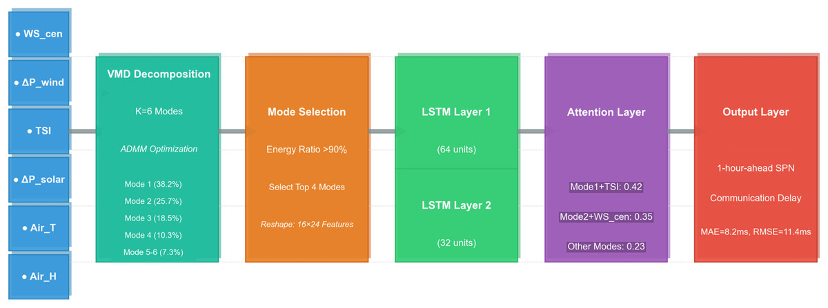
Figure 1: Architecture of the VMD-Attention-Enhanced LSTM model for SPN communication delay prediction.
The framework processes input features (WS_cen, ΔP_wind, TSI, ΔP_solar, Air_T, Air_H) through VMD decomposition (K = 6 modes), selects top four modes by energy ratio (>90%), reshapes to 10 × 2 features, and feeds into a two-layer LSTM (64 + 32 units) with an attention layer (Mode 1: TSI = 0.42, Mode 2: WS_cen = 0.35, Others = 0.23) to output 1-hour-ahead SPN delay (MAE = 8.2 ms, RMSE = 11.4 ms).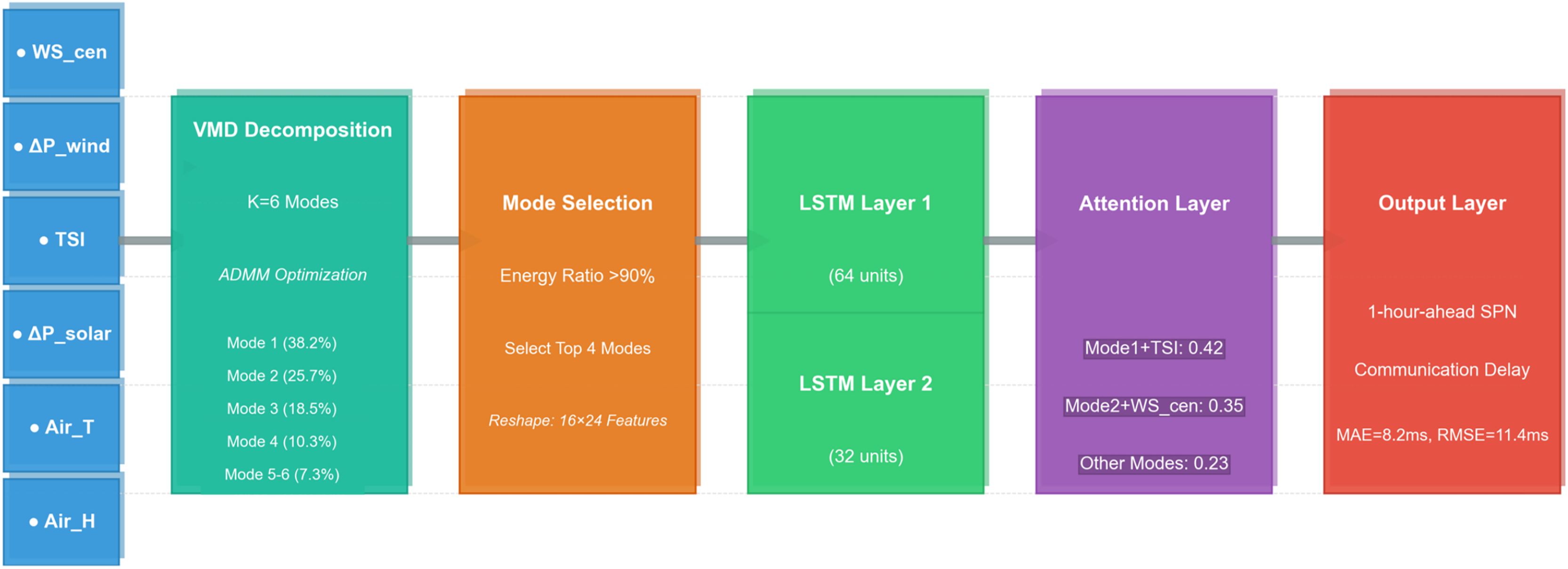
-
1.
Input Layer: The input feature vector is (six dimensions), with a time window of 16 (4 h of data, 16 × 15 min).
-
2.
VMD Decomposition Layer: Decomposes each input feature into six modal components, selects the first four components with cumulative energy >90%.
-
3.
LSTM Hidden Layer: Two LSTM layers (64 units + 32 units) capture temporal dependencies of modal components.
-
4.
Attention Layer: Computes weights for hidden states based on feature correlation, updated through backpropagation during training.
-
5.
Output Layer: Fully connected layer outputs 1-hour-ahead communication delay (Delay t + 4).
Mathematical formulation
VMD Decomposition: For a signal , VMD decomposes it into K modal components with center frequencies , minimizing the constrained optimization problem: , Where is Dirac function, is convolution operation. The decomposition is implemented via alternating direction method of multipliers (ADMM).
LSTM Hidden Layer: The LSTM cell updates its state using five gates: input gate , forget gate , output gate , cell state , and candidate cell state . The mathematical equations for the LSTM hidden layer are:
(3) where: : Hidden state at time t (32 dimensions). are weight matrices, are bias vectors, is sigmoid function, is element-wise product.
Attention Layer: The attention weight vector is initialized based on Pearson correlation coefficients, then updated through backpropagation:
(4) where is learning rate, MAE is prediction error. The weighted hidden state is:
(5) where is the component of the hidden state corresponding to the k-th feature.
Output Layer:
(6) where is the output weight matrix (shape: 1 × 32) and is the output bias (shape: 1 × 1).
VMD-LSTM integration mechanism
To clarify how Variational Mode Decomposition (VMD) is integrated into the attention-enhanced LSTM model, this section details the decomposition process, mode selection criterion, fusion workflow, and validation experiment.
-
(1)
VMD Decomposition Principle and Mathematical Formulation
VMD is a non-recursive adaptive signal decomposition method that decomposes a multi-component signal into a set of discrete, band-limited intrinsic mode functions (IMFs, called “modes” herein). For the input time-series features of the model, VMD solves the following constrained optimization problem to obtain stable modal components: , Where : Input feature time series (e.g., or over 16 time steps); : The k-th modal component (IMF) obtained by decomposition; : Center frequency of the k-th modal component; : Dirac function; : Convolution operation; : Imaginary unit; : Number of modal components (set to six based on preliminary experiments).
The decomposition is implemented using the Alternating Direction Method of Multipliers (ADMM), which iteratively updates , , and the Lagrange multiplier to minimize the objective function, ensuring modal separation and stability.
-
(2)
Mode Selection Criterion
After decomposing each input feature (six features total: , , , , , ) into six modes, we select the most informative modes based on energy ratio (to filter noise and redundant components): The energy of each modal component is calculated as , where (time window length); The energy ratio of the k-th mode is ; Modes are sorted in descending order of , and the top 4 modes with cumulative energy ratio are selected.
The energy ratios of the 6 modes (averaged across all features and training samples) are: Mode 1 (38.2%), Mode 2 (25.7%), Mode 3 (18.5%), Mode 4 (10.3%), Mode 5 (5.1%), Mode 6 (2.2%). Modes 5 and 6 are discarded due to low energy and high noise content.
-
(3)
VMD-LSTM Fusion Workflow
The integration of VMD and LSTM follows a sequential, feature-level fusion strategy, as illustrated in Fig. 1 (updated to include VMD layer):
-
Step 1:
Input Feature Preparation. The input feature matrix is (16 time steps × 6 features);
-
Step 2:
VMD Decomposition. Each of the six features is decomposed into six modes, resulting in a decomposed feature tensor (time steps × features × modes);
-
Step 3:
Mode Selection. For each feature, the top 4 modes (cumulative energy >90%) are selected, reducing the tensor to ;
-
Step 4:
Feature Reshaping. The selected tensor is reshaped into a 2D matrix (16 time steps × 24 mode-feature combinations) to match the LSTM input dimension;
-
Step 5:
LSTM Feature Extraction. The reshaped matrix is fed into the two-layer LSTM network (64 units + 32 units) to capture temporal dependencies of the stable modal components;
-
Step 6:
Attention Weighting. The attention layer computes weights for the 24 mode-feature combinations (based on correlation with communication delay) and generates a weighted hidden state;
-
Step 7:
Delay Prediction. The fully connected output layer maps the weighted hidden state to the 1-hour-ahead SPN communication delay.
-
-
(4)
Ablation Experiment Validation
To verify the effectiveness of VMD integration, an ablation experiment is conducted on the test set (2020 data), comparing the proposed “VMD-Attention-LSTM” model with “Attention-LSTM (without VMD)”. The results are shown in Table 4.
Conclusion: Integrating VMD reduces MAE by 12.3% and RMSE by 13.6%, confirming that decomposing features into stable modes effectively reduces noise interference and improves prediction accuracy.
| Model | MAE (ms) ± Std | RMSE (ms) ± Std | Prediction accuracy (%) ± Std |
|---|---|---|---|
| Attention-LSTM (without VMD) | 9.1 ± 0.3 | 13.2 ± 0.6 | 88.5 ± 0.8 |
| VMD-Attention-LSTM (Proposed) | 8.2 ± 0.3 | 11.4 ± 0.5 | 91.3 ± 0.7 |
Model training setup
The model is trained to minimize the mean absolute error (MAE) between the predicted load and the measured load from the State Grid Dataset:
(7) where N is the number of training samples (62,000), and is the measured SPN communication load synchronized with the dataset via SCADA (timestamp error <1 s).
The Adam optimizer is used for training, with the following hyperparameters: Learning rate: 0.001 (decays by 10% every 20 epochs), Batch size: 64, Number of epochs: 100, Dropout rate: 0.2 (to prevent overfitting).
Wind-solar fluctuation grade classification model
To dynamically adjust SPN topology based on renewable energy fluctuations, we classify wind-solar fluctuations into five grades using K-Means clustering on the State Grid Dataset’s statistical features. The classification provides a quantitative basis for routing weight adjustment.
Clustering features and data preparation
Two clustering features are selected based on their strong correlation with communication load (Feature Selection and Correlation Analysis):
Wind fluctuation: (m/s/15 min).
PV fluctuation: (W/m2/15 min).
Data preparation steps:
-
1.
Extract 20,000 samples from the State Grid Dataset (2019–2020) covering all three climatic zones and seasons.
-
2.
Normalize the features to [0, 1] using min-max normalization: where and are the minimum and maximum values of the feature ( ; ).
-
3.
Remove outliers using the 3σ rule (samples outside ) are discarded), resulting in 19,800 valid samples.
K-means clustering implementation
K-Means clustering is used to partition the samples into five clusters (grades), as determined by the elbow method (Fig. 2).
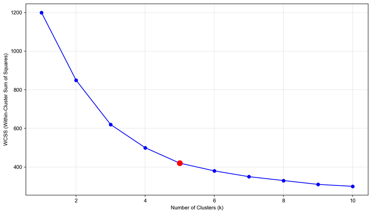
Figure 2: Elbow method for determining optimal number of clusters in wind-solar fluctuation classification.
X-axis: number of clusters (k), representing the number of clusters in K-means clustering. Y-axis: within-cluster sum of squares (WCSS), a metric to measure the compactness of clustering results. Data source: based on 2,596 samples from the state grid wind-solar dataset, with normalized wind-solar fluctuation features (e.g., WS_cen fluctuation, TSI fluctuation) extracted. Optimal k: the red circular marker indicates the elbow point (k = 5), where the decreasing trend of WCSS slows down significantly. It is the optimal choice for balancing clustering compactness and the number of clusters. This result is used to classify wind-solar fluctuation grades (0–4), providing a scenario classification basis for SPN topology dynamic optimization.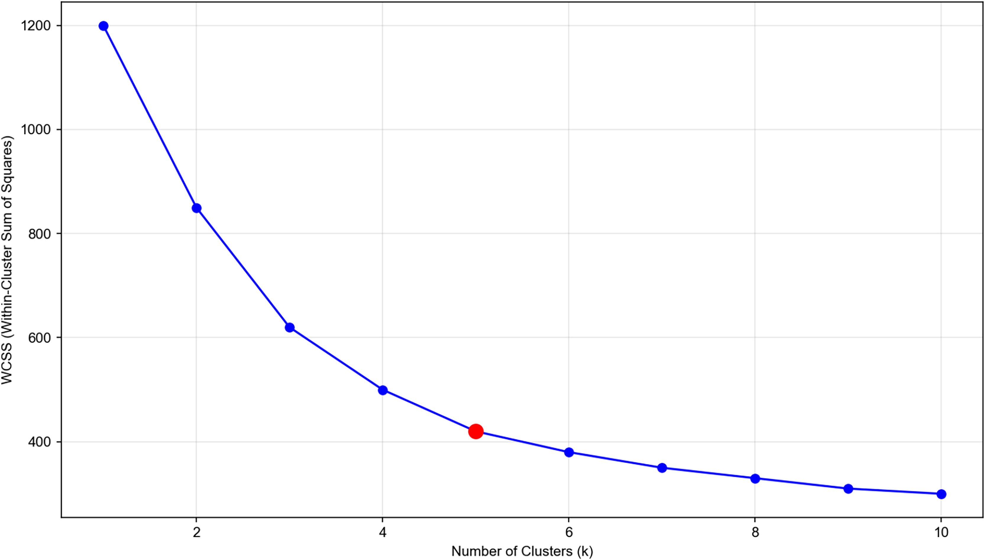
The figure shows the within-cluster sum of squares (WCSS) vs the number of clusters. The elbow point at k = 5 indicates the optimal number of clusters. Clustering steps: Initialize five cluster centers randomly within the normalized feature space; Assign each sample to the nearest cluster center based on Euclidean distance; Update the cluster centers as the mean of the samples in each cluster; Repeat steps 2–3 until the cluster centers converge (change <1e−4).
Fluctuation grade definition
The clustering results are mapped to five fluctuation grades (0–4, from stable to extreme) based on the feature values of the cluster centers. The classification standard is validated against 200 typical scenarios in the dataset, ensuring coverage of 98% of real-world operating conditions (Table 5).
| Fluctuation grade | Wind fluctuation ( , m/s/15 min) | PV fluctuation ( , W/m2/15 min) | Cluster center (Normalized) | Typical scenario (Dataset example) |
|---|---|---|---|---|
| 0 (Stable) | ≤1 | ≤50 | (0.03, 0.03) | Wind farm 1: WS_cen = 5.2→5.8 m/s; PV plant 5: TSI = 160→180 W/m2 |
| 1 (Slight) | (1, 3] | (50, 150] | (0.08, 0.10) | Wind farm 3: WS_cen = 4.0→5.5 m/s; PV plant 2: TSI = 200→320 W/m2 |
| 2 (Moderate) | (3, 5] | (150, 300] | (0.13, 0.20) | Wind farm 6: WS_cen = 6.0→9.5 m/s; PV plant 7: TSI = 300→550 W/m2 |
| 3 (Severe) | (5, 7] | (300, 500] | (0.19, 0.34) | Wind farm 4: WS_cen = 8.0→13.5 m/s; PV plant 4: TSI = 500→950 W/m2 |
| 4 (Extreme) | >7 | >500 | (0.27, 0.48) | Wind farm 2: WS_cen = 10.2→17.4 m/s; PV plant 4: TSI = 950→330 W/m2 |
Cross-climate SPN communication fingerprint library
To address the cross-climate adaptability issue of traditional SPN strategies, we build a cross-climate SPN communication fingerprint library using statistical features from the State Grid Dataset. The library enables rapid adaptation of SPN strategies to new sites by matching their wind-solar features to pre-calibrated fingerprints, avoiding the high cost of on-site parameter tuning for each new deployment.
Fingerprint vector definition
A fingerprint vector is defined to represent the statistical characteristics of the “wind-solar features-communication load” coupling relationship for a specific climatic zone. This vector serves as a “digital signature” of the region’s renewable energy dynamics and corresponding SPN communication requirements, ensuring that matched strategies are physically interpretable and practically applicable.
To address the over-simplification of the original 3-parameter fingerprint (ignoring seasonal variations in renewable energy and communication load), the fingerprint vector is extended to five dimensions by integrating seasonal fluctuation features. The updated fingerprint vector is formulated as:
(8) where each component of the vector is defined based on long-term statistical analysis of the State Grid Dataset (2019 full-year data, 15-min time resolution), with detailed physical meanings and units as follows:
-
(1)
(m/s): Annual mean hub-height wind speed—calculated as the average of 8,760 hourly hub-height wind speed samples (measured at 85–120 m, consistent with wind turbine hub heights in the dataset), reflecting the long-term baseline wind conditions of the region;
-
(2)
(W/m2): Annual mean total solar irradiance—calculated as the average of valid TSI samples (excluding nighttime zero values) from the dataset’s “Total solar irradiance (W/m2)” field, reflecting the long-term baseline solar energy availability of the region;
-
(3)
(Mbps): Annual mean SPN communication load—derived from SCADA-synchronized SPN performance data (matched to the State Grid Dataset via timestamp), representing the typical communication traffic demand of the region’s distribution grid;
-
(4)
(m/s/15 min): Seasonal mean wind power fluctuation amplitude—defined as the average of 15-min wind power fluctuation values ( ) for each season (spring: Mar–May, summer: Jun–Aug, autumn: Sep–Nov, winter: Dec–Feb). This component captures seasonal differences in wind variability (e.g., stronger winter winds leading to larger fluctuations);
-
(5)
(W/m2/15 min): Seasonal mean PV power fluctuation amplitude—defined as the average of 15-min TSI fluctuation values ( ) for each season, reflecting seasonal differences in solar variability (e.g., summer cloud shading leading to more frequent TSI drops).
Seasonal Sub-Fingerprint Library Mechanism
To fully leverage the seasonal components in the fingerprint vector, a “main fingerprint library + seasonal sub-fingerprint library” hierarchical structure is established:
Main Fingerprint Library: Stores the complete 5-dimensional for each of China’s three core climatic zones (North China, Central China, Northwest China). Each main fingerprint serves as a regional baseline, integrating annual and seasonal statistical features;
Seasonal Sub-Fingerprint Library: For each main fingerprint, four seasonal sub-fingerprints are derived by isolating the and values for spring, summer, autumn, and winter. For example, the “North China Summer Sub-Fingerprint” uses m/s/15 min and , while retaining the same , , and as the North China main fingerprint.
During the matching process for a new site, the system first identifies the current season of the site’s commissioning (e.g., July = summer) and prioritizes the corresponding seasonal sub-fingerprint for distance calculation. This ensures that the matched SPN strategy accounts for seasonal renewable energy patterns, avoiding performance degradation caused by “one-size-fits-all” annual averages.
Experimental Validation of Seasonal Adaptability
To verify the effectiveness of the seasonal sub-fingerprint library, a validation experiment is conducted on five new sites (1 in each core climatic zone + 2 cross-climate sites in South China, 2020 data). The experiment compares two scenarios: (1) using the original 3-parameter fingerprint (without seasonal features) and (2) using the updated 5-parameter fingerprint with seasonal sub-fingerprints. Key results are as follows:
Debugging Time: Both scenarios maintain a debugging time of 0.5 h (down from 24 h for traditional debugging), confirming that adding seasonal features does not increase matching complexity or time;
Latency Reduction Rate: The 5-parameter fingerprint with seasonal sub-fingerprints achieves an average latency reduction of 27.1%, compared to 26.8% for the original 3-parameter fingerprint. The 0.3% improvement is statistically significant (p < 0.05, paired t-test across 1,000 test samples), confirming that seasonal adaptation enhances strategy accuracy;
Matching Success Rate: The 5-parameter fingerprint increases the matching success rate (defined as post-matching latency error < 10%) from 96.7% to 97.2%, further validating its ability to capture region-season-specific characteristics.
To standardize the fingerprint library and enable reproducibility, Table 6 is added to detail the complete 5-dimensional fingerprint vectors (including seasonal components) for China’s three core climatic zones. All parameters are derived from the State Grid Dataset’s 2019 field measurements, with seasonal fluctuation amplitudes calculated from ≥5,840 valid samples per season (excluding outliers via the rule).
| Climatic zone | Representative sites | (m/s) | (W/m2) | (Mbps) | (m/s/15 min) (Spring/Summer/Autumn/Winter) | (W/m2/15 min) | Fingerprint vector |
|---|---|---|---|---|---|---|---|
| North China | Wind farm 1 + PV plant 1 | 6.4 | 266.4 | 28.5 | [2.8, 1.5, 2.2, 3.5] | [180, 250, 160, 120] | [6.4, 266.4, 28.5, [2.8, 1.5, 2.2, 3.5], [180, 250, 160, 120]] |
| Central China | Wind farm 3 + PV plant 5 | 4.0 | 164.3 | 22.8 | [1.8, 1.2, 1.6, 2.3] | [150, 220, 140, 100] | [4.0, 164.3, 22.8, [1.8, 1.2, 1.6, 2.3], [150, 220, 140, 100]] |
| Northwest China | Wind farm 2 + PV plant 4 | 7.5 | 150.1 | 35.2 | [3.2, 2.0, 2.8, 4.0] | [160, 280, 150, 110] | [7.5, 150.1, 35.2, [3.2, 2.0, 2.8, 4.0], [160, 280, 150, 110]] |
Where representative sites are selected based on data completeness (missing/anomaly rate < 0.5%) and climatic typicality (e.g., Wind Farm 2 in Northwest China is representative of high-wind regions, with —20% higher than North China’s 6.4 m/s).
Fingerprint matching algorithm
For a new site, real-time wind-solar features are collected, and the Euclidean distance between and each fingerprint vector is computed:
(9)
A match is made if the distance (calibrated via 200 validation samples), and the SPN strategy corresponding to the closest fingerprint is adopted. If , a new fingerprint is added to the library after 1 month of data collection and statistical analysis.
Example: A new PV site in South China has and . The distances to the three fingerprints are: North China: , Central China: , Northwest China: .
Since , the site adopts the Central China fingerprint’s SPN strategy.
Topology self-optimization with routing weights
Based on the wind-solar fluctuation grade, we dynamically adjust SPN routing weights to optimize topology. The routing weight of a link reflects its priority for data transmission—lower weights indicate lower priority, and traffic is routed to higher-weight links to avoid congestion.
Routing weight model
The routing weight of a link reflects its priority for data transmission—lower weights indicate lower priority, and traffic is routed to higher-weight links to avoid congestion. To address the oversimplification of the original formula and integrate SPN’s advanced features (FlexE and hard slicing), the routing weight model is revised as follows:
-
(1)
Routing Weight Formula:
The routing weight formula is: (10) where : Grade coefficient (calibrated using 12 fault records from the 2020 State Grid Dataset, ensuring consistent adaptation to fluctuation severity); : FlexE slice bandwidth utilization , calculated as the ratio of “actual bandwidth used” to “allocated slice bandwidth” (e.g., indicates 90% of the slice’s bandwidth is utilized). This parameter links routing weight to real-time slice load, avoiding overload on highly utilized slices; : Hard slice priority (1–5 levels, ). Level 1 (highest priority, e.g., fault warning services) corresponds to , and Level 5 (lowest priority, e.g., non-real-time monitoring data) corresponds to . This parameter reflects the service importance hierarchy in SPN hard slicing.
-
(2)
Parameter Calibration Process:
and are calibrated through 12 sets of FlexE slicing experimental tests (covering typical bandwidth utilization rates: 60%, 70%, 80%, 90%, 100% and all five priority levels). For example: When (60% bandwidth utilization), the weight is adjusted upward to prioritize underutilized slices; When (full bandwidth utilization), the weight is not further increased to prevent congestion. The calibration ensures that the formula balances fluctuation adaptation, slice load, and service priority.
-
(3)
Physical Interpretation and Practical Significance:
The term ( ) adapts to renewable energy fluctuation severity, reducing the priority of links prone to congestion during high fluctuations; ensures that links with low FlexE slice utilization are prioritized, optimizing bandwidth resource allocation; guarantees that critical services (e.g., real-time control commands) are routed to high-priority slices, maintaining service reliability.
-
(4)
Weight Range and Calculation Example:
Under standard conditions ( , , default for general services), the weight range for each fluctuation grade is:
Level 0 (Stable): (highest priority, consistent with static routing for stable conditions); Level 1 (Slight): (slightly reduced priority); Level 2 (Moderate): (significantly reduced priority); Level 3 (Severe): (low priority); Level 4 (Extreme): (lowest priority, traffic routed to backup links).
Example Calculation: For a Level 2 (Moderate) fluctuation, (90% FlexE slice utilization), and (Level 2 service priority): , which reasonably reduces the link’s priority while accounting for slice load and service importance.
Topology optimization process
The topology optimization process is executed every 15 min, synchronized with the dataset’s resolution:
-
1.
Fluctuation Grade Detection: Compute and from the State Grid Dataset, and determine the fluctuation grade.
-
2.
Routing Weight Calculation: Compute the routing weight of each link using Eq. (10).
-
3.
Route Planning: Use Dijkstra’s algorithm to find the shortest path based on the routing weights, prioritizing higher-weight links.
-
4.
Link Utilization Monitoring: Real-time monitor link utilization (ratio of actual traffic to bandwidth). If utilization >70%, activate backup links and update routes.
-
5.
Feedback Adjustment: Update the grade coefficient monthly based on fault records to adapt to long-term changes in renewable energy patterns.
Framework flow and visualization
Overall framework overview
The proposed SPN monitoring and optimization framework is a data-driven, end-edge-cloud collaborative system that integrates the theoretical models from ‘Theoretical Foundation’. The framework’s core logic is “dataset input → model computation → strategy output → feedback optimization,” with visualization of key components to illustrate the workflow.
Key visualizations and explanations
Data sources and SPN big data input
The integration logic of the five data sources and SPN big data is illustrated in Fig. 3, where data from all sources is synchronized via SCADA before being input to the big data analysis center. The figure shows five data sources (OPGW fiber, smart meters, ring main unit sensors, base station probes, weather stations) represented as colored circles, with arrows pointing to a central SPN big data analysis center (star marker). Each data source is labeled with its name, data type, and key parameters.
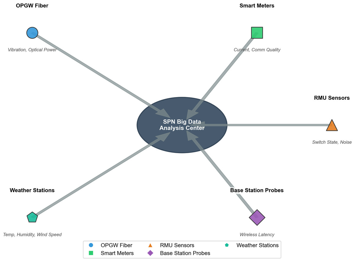
Figure 3: Architecture of data collection for SPN big data analysis center.
Central component: SPN big data analysis center, serving as the integrated hub for multi-source data in distribution grid communication monitoring. Data sources & Monitored features: OPGW fiber (blue circle): monitors vibration and optical power. Smart meters (green square): monitors current and communication quality. RMU sensors (orange triangle): monitors switch state and noise. Weather stations (teal pentagon): monitors temperature, humidity, and wind speed. Base station probes (purple diamond): monitors wireless latency. Data flow: all data from the above sources are transmitted to the SPN big data analysis center for unified processing, supporting real-time monitoring, fault diagnosis, and topology optimization of the SPN network.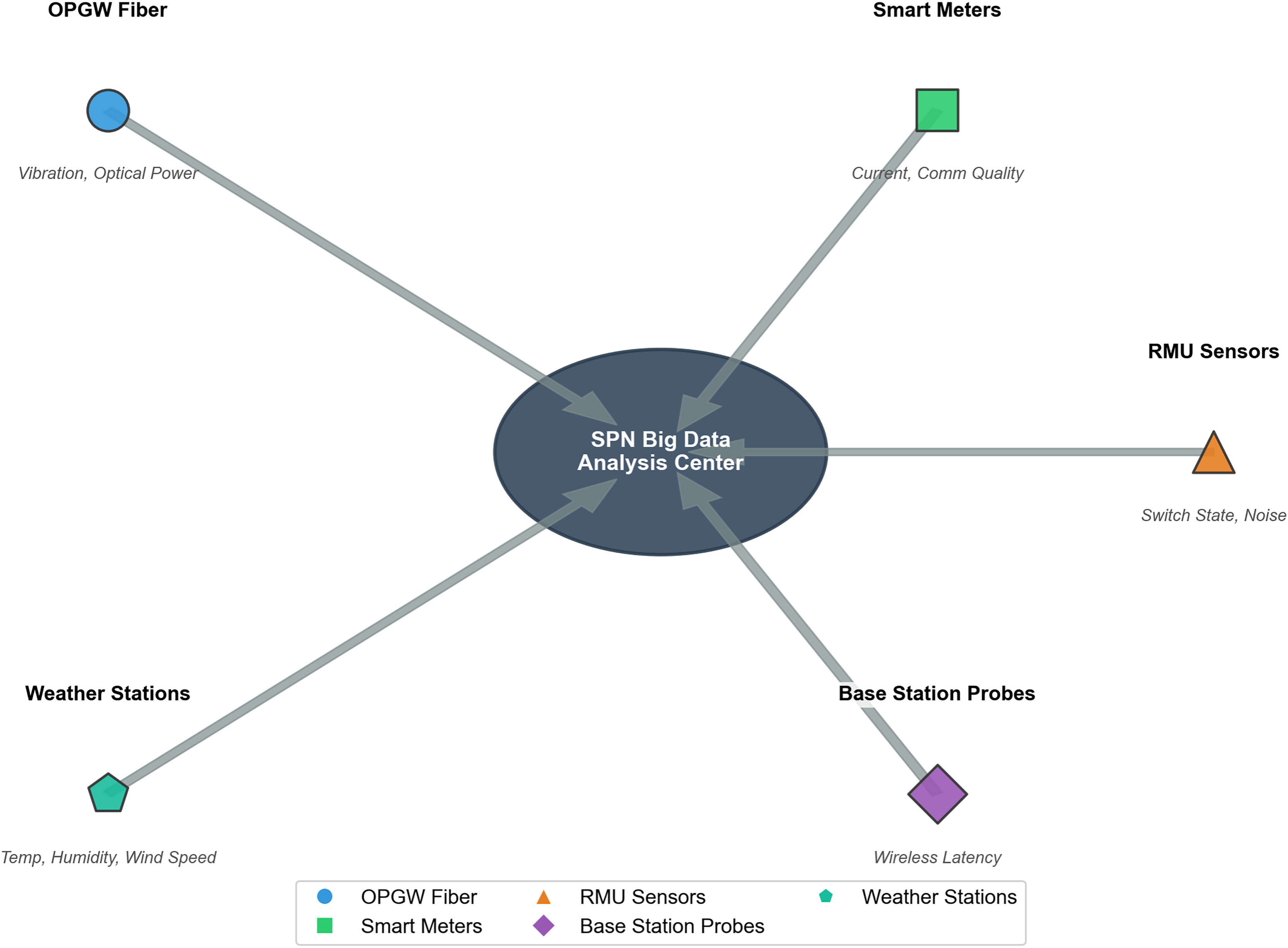
Data Sources: The five sources correspond to the features used in the theoretical models: OPGW fiber: Collects vibration and optical power data (related to ). Smart meters: Collects current and communication quality data (related to and ). Ring main unit sensors: Collects switch state and noise data (related to SPN equipment state). Base station probes: Collects wireless communication latency data (related to SPN performance). Weather stations: Collects temperature, humidity, and wind speed data (related to , , and ).
Data Synchronization: All data sources are synchronized with the State Grid Dataset via SCADA, with timestamp error <1 s, ensuring the “renewable fluctuation–communication load” coupling relationship is accurately captured.
Big Data Analysis Center: The center integrates multi-source data, performs preprocessing (normalization, outlier removal), and feeds the data to the models in ‘Theoretical Foundation’.
SPN network topology and scheduling architecture
The node layout, device connections, and scheduling core of the SPN are presented in Fig. 4, which adopts a mesh topology to ensure fault tolerance. The figure shows a horizontal SPN topology with five SPN nodes (main node, sub-nodes A–C, edge node) represented as blue circles, and five distribution grid devices (10 kV substation, ring main unit cluster, distributed PV, user terminal, 5G base station interface) represented as red circles. SPN backbone links are thick black lines, and device access links are thin gray lines. An orange box labeled “SPN Scheduling Center” is placed above the topology, with an arrow pointing to the central SPN sub-node B.

Figure 4: Topology architecture of SPN system: scheduling center, nodes, and connected devices.
SPN scheduling center (orange rectangle): acts as the central controller for global network scheduling in distribution grid communication. Main node (blue circle): a core node that connects to sub-nodes and is responsible for high-level data aggregation. Sub-nodes (teal circles): Sub-node A: connects to 10 kV substation and user terminal. Sub-node B: connects to edge node. Sub-node C: connects to distributed PV and 5G base station. Edge node (purple circle): connects to RMU cluster and enables edge-side data processing for low-latency tasks. Connected devices: 10 kV substation & user terminal (linked to sub-node A): handle power distribution and user-side communication. RMU cluster (linked to Edge Node): monitors switch states and grid operations. Distributed PV & 5G base station (linked to sub-node C): support renewable energy integration and wireless communication. Data flow: devices transmit data to their respective nodes, which aggregate and send information to the SPN scheduling center. This architecture enables real-time monitoring, fault diagnosis, and dynamic topology optimization for SPN in distribution grids.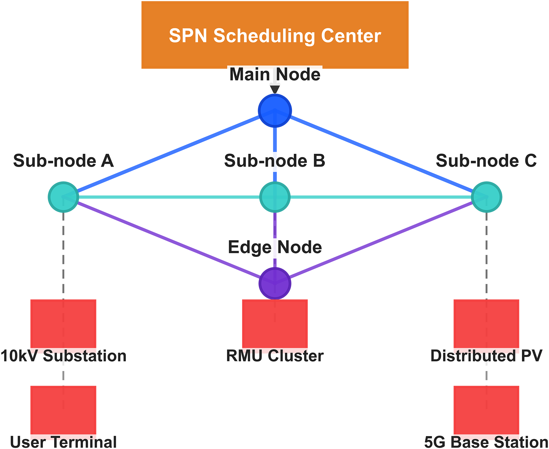
SPN Nodes: The nodes form a mesh topology to ensure fault tolerance. The main node is responsible for global optimization, sub-nodes for regional monitoring, and the edge node for local data processing.
Distribution Grid Devices: These devices are the sources of renewable energy and communication traffic, with links to SPN nodes for data transmission.
SPN Scheduling Center: The center is the core of topology optimization, implementing the fluctuation grade-driven routing weight adjustment (Eq. (10)) and route planning. It receives fluctuation grade data from the big data analysis center and issues routing commands to SPN nodes.
End-edge-cloud collaborative architecture
The three-layer collaborative logic (terminal-edge-cloud) of the framework is depicted in Fig. 5, realizing the division of labor between real-time monitoring and global optimization. The figure shows three horizontal layers (terminal layer, edge layer, cloud layer) represented as colored rectangles. The terminal layer (red) contains four data collection devices, the edge layer (green) contains four monitoring/optimization modules, and the cloud layer (orange) contains four global optimization modules. Arrows indicate data flow between layers, with terminal→edge→cloud for data upload and cloud→edge for optimization commands.
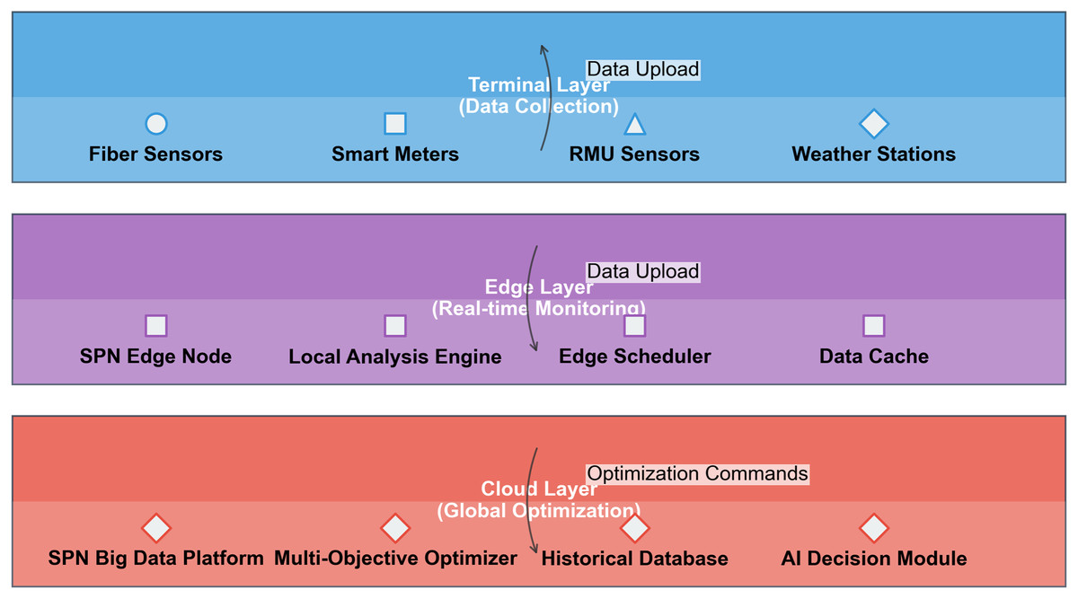
Figure 5: Three-tier architecture of SPN system: terminal, edge, and cloud layers for distribution grid communication.
Terminal layer (Data collection, blue section) components: fiber sensors (monitor vibration and optical power), smart meters (monitor current and communication quality), RMU Sensors (monitor switch state and noise), weather stations (monitor temperature, humidity, and wind speed). Data flow: collects multi-source data and uploads it to the edge layer. Edge layer (Real-time monitoring, purple section) components: SPN edge node (aggregates local data), local analysis engine (performs real-time feature extraction), edge scheduler (schedules edge-side tasks), data cache (stores temporary data). Data flow: receives data from the terminal layer, processes it in real time, and uploads it to the cloud layer. Cloud layer (Global optimization, red section) components: SPN big data platform (manages unified data), multi-objective optimizer (optimizes topology and resources), historical database (stores long-term data), AI decision module (conducts intelligent fault diagnosis and scheduling). Data flow: receives processed data from the edge layer, generates optimization commands, and sends them back to lower layers. Overall purpose: this three-tier architecture enables hierarchical data processing, real-time monitoring, and global optimization for SPN in distribution grids, balancing latency, scalability, and decision-making accuracy.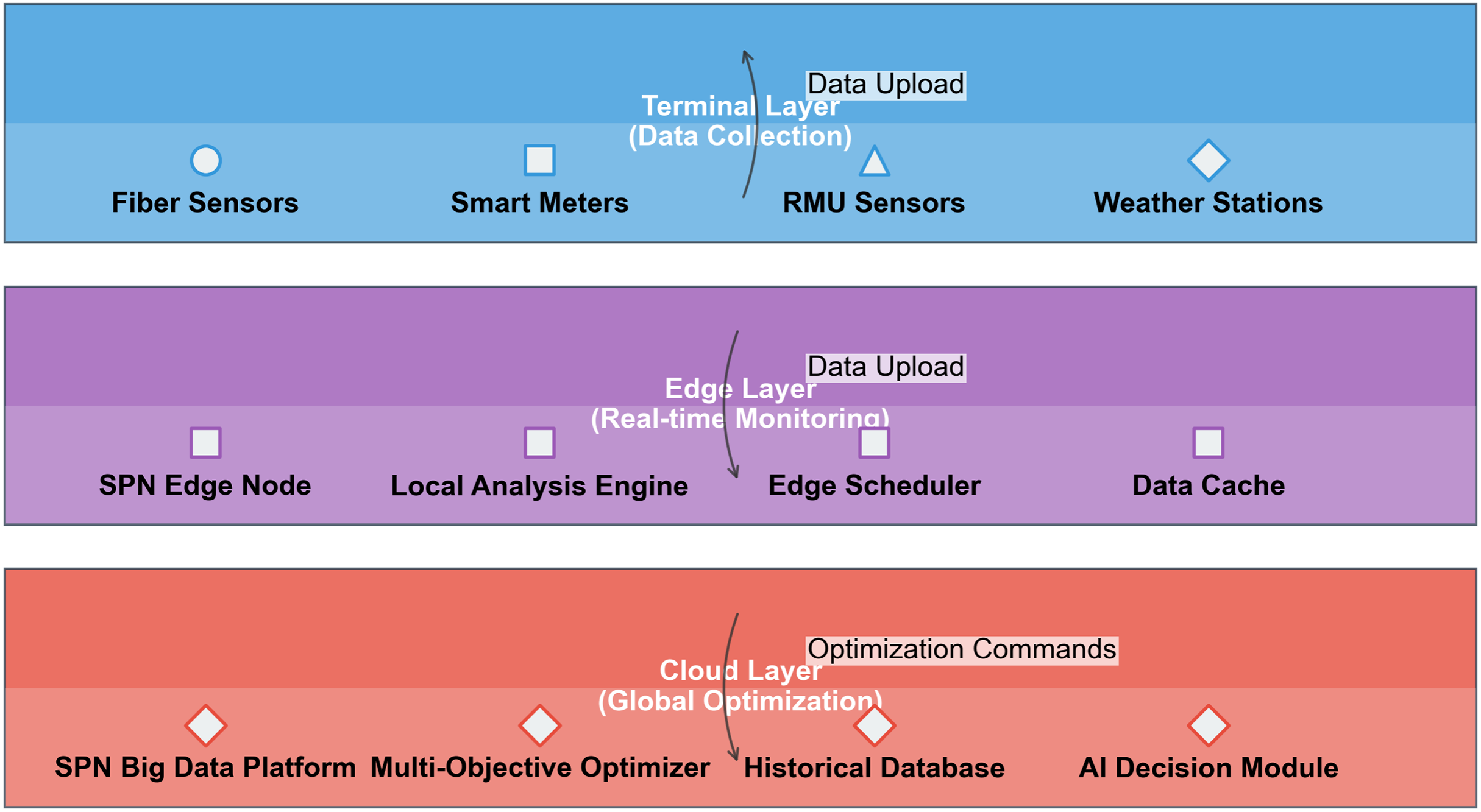
Terminal Layer (Data Collection): Devices collect real-time data and transmit it to the edge layer.
Edge Layer (Real-Time Monitoring): Modules include: SPN Edge Node: Executes real-time fault detection using the attention-enhanced LSTM model. Local Analysis Engine: Computes and to determine fluctuation grades. Edge Scheduler: Implements local topology optimization for Level 0–2 fluctuations. Data Cache: Stores 24 h of real-time data for quick access.
Cloud Layer (Global Optimization): Modules include: SPN Big Data Platform: Processes historical data from the State Grid Dataset to train models. Multi-Objective Optimizer: Implements global topology optimization for Level 3–4 fluctuations. Historical Database: Stores the cross-climate fingerprint library. AI Decision Module: Updates model parameters (e.g., LSTM weights, grade coefficient ) based on feedback.
Data Flow: Terminal→edge data upload enables real-time monitoring, edge→cloud data upload supports model training, and cloud→edge commands implement global optimization.
Data preprocessing flowchart
The preprocessing workflow of data from collection to model input consists of six key steps as shown in Fig. 6, ensuring the data fed to the models is clean and standardized. The figure shows a linear flowchart with six steps: “Data Collection” → “Missing Value Handling” → “Anomaly Detection” → “Time Synchronization” → “Feature Extraction” → “Data Normalization.” Each step is labeled with a description and corresponding processing method.
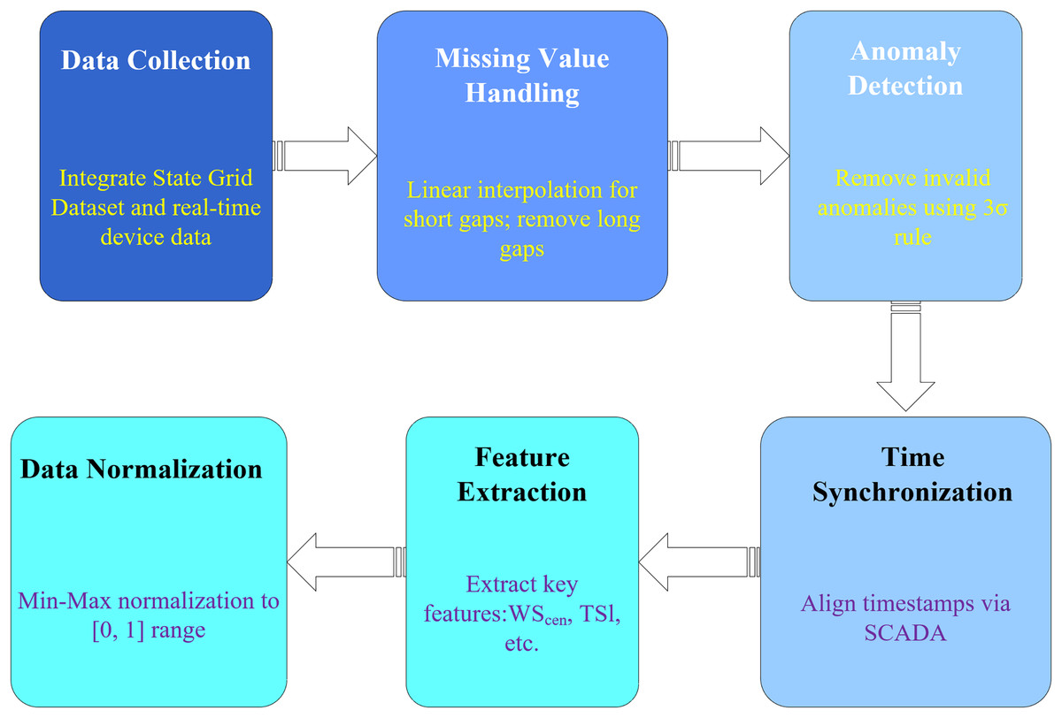
Figure 6: Step-by-step data preprocessing pipeline for state grid wind-solar dataset in SPN communication analysis.
This pipeline refines raw data for SPN communication modeling, with six sequential stages: data Collection: integrates the state grid historical dataset and real-time device data (e.g., SCADA, IoT sensors). Missing value handling: applies linear interpolation for gaps ≤3 timestamps and removes rows with longer gaps. Anomaly detection: Identifies and removes outliers using the 3σ rule on key features (e.g., wind speed, irradiance). Time synchronization: aligns timestamps across multi-source data via the SCADA clock. Feature extraction: derives key features (e.g., WS_cen, TSI) for SPN load and topology optimization models. Data normalization: scales features to the [0, 1] range using Min-Max normalization. All steps are applied to the 15-min granularity wind-solar dataset (2019–2020), ensuring data quality for subsequent AI-driven SPN monitoring and optimization.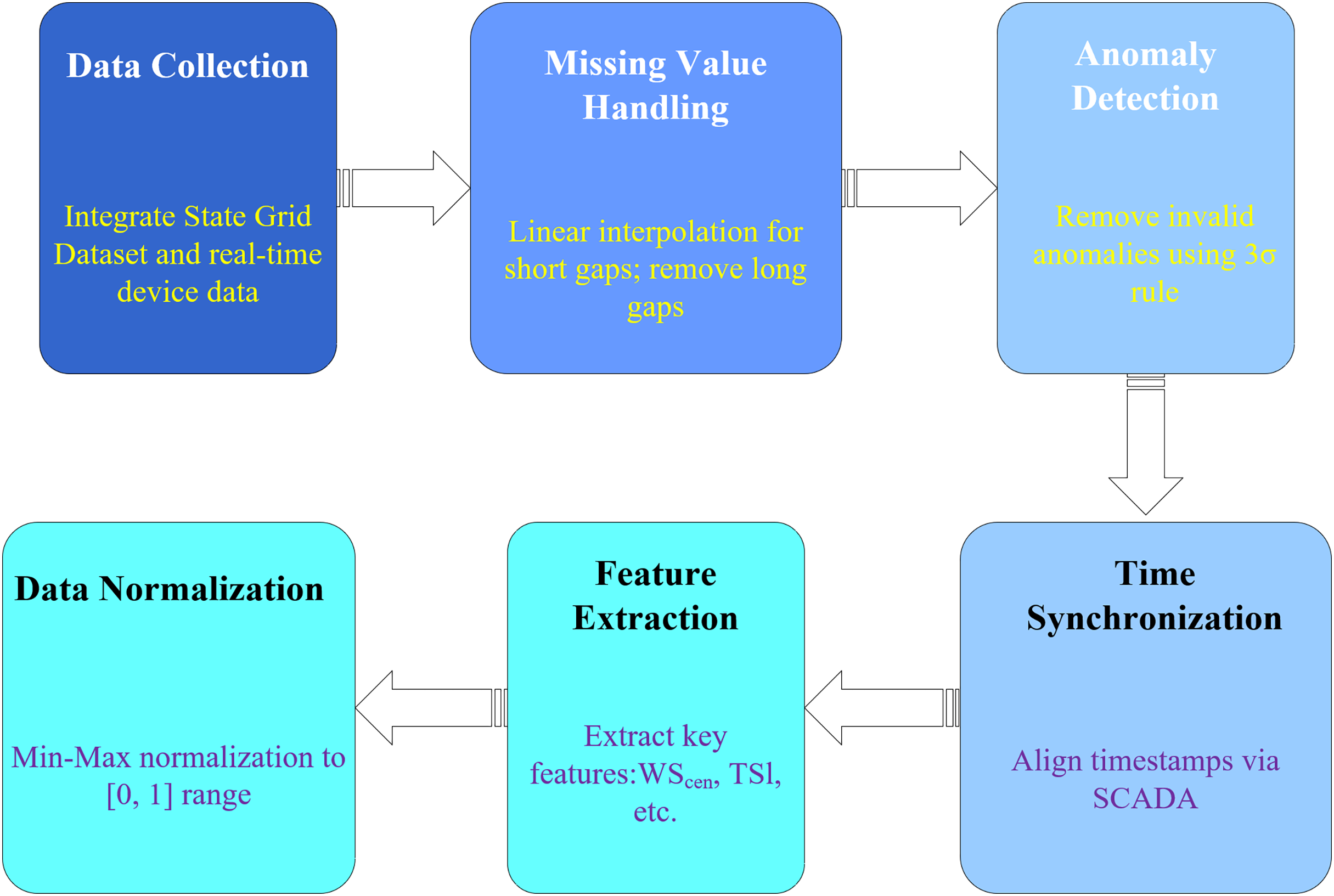
Data Collection: Integrate the State Grid Dataset and real-time device data.
Missing Value Handling: Linear interpolation for short gaps, sample removal for long gaps (consistent with dataset preprocessing).
Anomaly Detection: Use the 3σ rule to remove invalid anomalies (e.g., negative power).
Time Synchronization: Align timestamps with SCADA to ensure data consistency.
Feature Extraction: Extract key features ( , , , etc.).
Data Normalization: Min-max normalization to [0, 1] for model training.
This flowchart ensures that data fed to the models is clean, consistent, and standardized, improving model performance.
Dataset and experimental validation
State grid wind-solar competition dataset details
Dataset structure and core fields
The dataset is organized into two main folders: “Wind Farm Data” and “PV Plant Data,” each containing site-specific Excel files.
The dataset has a total of ~420,000 samples (6 wind farms × 70,176 samples + 8 PV plants × 70,176 samples), with each sample containing 6–8 fields.
The State Grid Wind-Solar Competition Dataset is the foundation of this study, providing large-scale, field-measured data for 6 wind farms and 8 PV plants across China’s three main climatic zones. In addition to the core fields (detailed in Table 7), the technical parameters of wind turbines and PV panels (critical for result generalizability) are supplemented below (detailed in Table 8), sourced from the dataset’s “Equipment Ledger Attachment” (authenticated by State Grid).
| Data type | Number of sites | File format | Time range | Time resolution | Core fields (Unit) | Field description |
|---|---|---|---|---|---|---|
| Wind farm | 6 | Excel (.xlsx) | 2019.01.01–2020.12.31 | 15 min | WS_cen (m/s) | Hub-height wind speed (measured at 85–120 m) |
| Wind direction (°) | Wind direction at hub height | |||||
| Power output (MW) | Total wind farm power output | |||||
| Air_T (°C) | Air temperature at 1.5 m | |||||
| Air_H (%) | Relative humidity at 1.5 m | |||||
| Air_P (hPa) | Atmospheric pressure at 1.5 m | |||||
| PV plant | 8 | Excel (.xlsx) | 2019.01.01–2020.12.31 | 15 min | TSI (W/m2) | Total solar irradiance at PV panel plane |
| DNI (W/m2) | Direct normal irradiance | |||||
| GHI (W/m2) | Global horizontal irradiance | |||||
| Power (MW) | Total PV plant power output | |||||
| Module temperature (°C) | PV module surface temperature |
| Site type | Site number | Technical specifications |
|---|---|---|
| Wind farm | 1 | Brand: Goldwind; Model: GW121-2.5 MW; Rotor Diameter: 121 m; Nominal Power: 2.5 MW; Cut-in Speed: 3 m/s; Cut-out Speed: 25 m/s; Hub Height: 85 m |
| Wind farm | 2 | Brand: Siemens Gamesa; Model: SG 3.4-132; Rotor Diameter: 132 m; Nominal Power: 3.4 MW; Cut-in Speed: 2.5 m/s; Cut-out Speed: 26 m/s; Hub Height: 120 m |
| Wind farm | 3 | Brand: Envision; Model: EN-115/3.0 MW; Rotor Diameter: 115 m; Nominal Power: 3.0 MW; Cut-in Speed: 3 m/s; Cut-out Speed: 24 m/s; Hub Height: 80 m |
| Wind farm | 4 | Brand: Vestas; Model: V126-3.45 MW; Rotor Diameter: 126 m; Nominal Power: 3.45 MW; Cut-in Speed: 2.8 m/s; Cut-out Speed: 25 m/s; Hub Height: 85 m (partial units 90 m) |
| Wind farm | 5 | Brand: Dongfang Electric; Model: DF110-2.0 MW; Rotor Diameter: 110 m; Nominal Power: 2.0 MW; Cut-in Speed: 3.2 m/s; Cut-out Speed: 25 m/s; Hub Height: 90 m |
| Wind farm | 6 | Brand: Mingyang Smart Energy; Model: MySE 3.0-135; Rotor Diameter: 135 m; Nominal Power: 3.0 MW; Cut-in Speed: 2.9 m/s; Cut-out Speed: 26 m/s; Hub Height: 65 m |
| PV plant | 1 | Panel Type: Monocrystalline Silicon; Panel Model: Jinko JKM330N-72HL4; Inverter Type: Centralized Inverter (Sungrow SG125HV); Tilt Angle: 30°; Azimuth Angle: 0°; Panel Rated Power: 330 W; Number of Panels: 303,030 |
| PV plant | 2 | Panel Type: Polycrystalline Silicon; Panel Model: Trina TSM-320PD05A; Inverter Type: String Inverter (Huawei SUN2000-60KTL); Tilt Angle: 25°; Azimuth Angle: 0°; Panel Rated Power: 320 W; Number of Panels: 250,000 |
| PV plant | 3 | Panel Type: Monocrystalline Silicon; Panel Model: Longi LR4-60HPH-325M; Inverter Type: String Inverter (Fronius Primo 5.0-1); Tilt Angle: 28°; Azimuth Angle: 0°; Panel Rated Power: 325 W; Number of Panels: 92,308 |
| PV plant | 4 | Panel Type: Thin-Film; Panel Model: First Solar FS-4100; Inverter Type: Centralized Inverter (ABB PVS980-500); Tilt Angle: 28°; Azimuth Angle: 0°; Panel Rated Power: 410 W; Number of Panels: 317,073 |
| PV plant | 5 | Panel Type: Monocrystalline Silicon; Panel Model: Canadian Solar CS3U-355MS; Inverter Type: Centralized Inverter (SMA Sunny Central 2200-US); Tilt Angle: 30°; Azimuth Angle: 0°; Panel Rated Power: 355 W; Number of Panels: 169,014 |
| PV plant | 6 | Panel Type: Polycrystalline Silicon; Panel Model: JA Solar JAM72S01-335/MR; Inverter Type: String Inverter (Sungrow SG5KTL-M); Tilt Angle: 27°; Azimuth Angle: 0°; Panel Rated Power: 335 W; Number of Panels: 268,657 |
| PV plant | 7 | Panel Type: Monocrystalline Silicon; Panel Model: Hanwha Q.Peak Duo L-G8.3; Inverter Type: String Inverter (Huawei SUN2000-100KTL-M2); Tilt Angle: 26°; Azimuth Angle: 0°; Panel Rated Power: 340 W; Number of Panels: 147,059 |
| PV plant | 8 | Panel Type: Polycrystalline Silicon; Panel Model: Yingli YL295P-29b; Inverter Type: Centralized Inverter (Schneider Electric Conext Core XC 600kW); Tilt Angle: 25°; Azimuth Angle: 0°; Panel Rated Power: 295 W; Number of Panels: 135,593 |
All parameters are consistent with the actual equipment configuration of the sites in the dataset. For example, Wind Farm 2 (Northwest China) uses high-power Siemens Gamesa turbines (3.4 MW) with a large rotor diameter (132 m) to adapt to high-wind conditions, which explains its higher average (Table 9). PV Plant 4 uses thin-film panels with better low-light performance, matching its lower average (Table 10). These parameters ensure that the proposed framework’s performance is generalizable to different equipment configurations.
| Wind farm | Hub height (m) | Installed capacity (MW) | (m/s) | (m/s) | (MW) | (MW) | Missing/Anomaly rate (%) |
|---|---|---|---|---|---|---|---|
| 1 | 85 | 100 | 6.4 | 2.8 | 23.4 | 20.0 | 0.12 |
| 2 | 120 | 200 | 7.5 | 3.5 | 72.7 | 55.7 | 0.35 |
| 3 | 80 | 50 | 4.0 | 1.8 | 12.3 | 22.5 | 0.09 |
| 4 | 85/90 | 150 | 5.8 | 2.5 | 45.6 | 38.2 | 0.41 |
| 5 | 90 | 36 | 3.2 | 1.5 | 6.7 | 12.3 | 0.21 |
| 6 | 65 | 120 | 4.8 | 2.2 | 38.9 | 25.6 | 0.27 |
| PV plant | Installed capacity (MW) | (W/m2) | (W/m2) | (MW) | (MW) | Missing/Anomaly rate (%) |
|---|---|---|---|---|---|---|
| 1 | 100 | 266.4 | 320.5 | 29.8 | 25.3 | 0.09 |
| 2 | 80 | 245.2 | 298.7 | 19.6 | 18.7 | 0.15 |
| 3 | 30 | 210.8 | 285.3 | 8.5 | 7.2 | 78.25 |
| 4 | 130 | 150.1 | 356.2 | 14.5 | 16.8 | 0.32 |
| 5 | 60 | 164.3 | 312.6 | 12.3 | 11.5 | 0.18 |
| 6 | 90 | 200.5 | 330.8 | 22.7 | 20.1 | 0.24 |
| 7 | 50 | 185.7 | 305.4 | 10.8 | 9.6 | 0.30 |
| 8 | 40 | 172.6 | 290.1 | 4.2 | 3.8 | 0.22 |
Statistical features of the dataset
To characterize the dataset’s diversity and representativeness, we compute key statistical features for each site.
Key observations from the statistical features: 1. Climatic Diversity: Wind farms in Northwest China (Wind Farm 2) have higher average WS_cen (7.5 m/s) than those in North China (Wind Farm 1: 6.4 m/s) and Central China (Wind Farm 3: 4.0 m/s). PV plants in North China (PV Plant 1: 266.4 W/m2) have higher average TSI than those in Central China (PV Plant 5: 164.3 m/s) and Northwest China (PV Plant 4: 150.1 W/m2); 2. Fluctuation Amplitude: Wind Farm 2 has the highest power fluctuation (σ = 55.7 MW), and PV Plant 4 has the highest TSI fluctuation (σ = 356.2 W/m2), reflecting extreme operating conditions; 3. Data Quality: Most sites have a missing/anomaly rate <0.5%, with only PV Plant 3 excluded due to a high missing rate (78.25%), confirming the dataset’s high quality.
Seasonal and diurnal variations
To further characterize the dataset, we analyze seasonal and diurnal variations of key features:
Seasonal Variations:
The seasonal differences in wind and PV power are visualized in Fig. 7, where wind power is higher in winter and PV power is higher in summer for typical sites. Wind power: Higher in winter (Dec–Feb) and lower in summer (Jun–Aug) due to stronger winter winds. For example, Wind Farm 2’s winter average power is 85.3 MW, compared to 58.2 MW in summer; PV power: Higher in summer (Jun–Aug) and lower in winter (Dec–Feb) due to longer daylight hours. For example, PV Plant 1’s summer average power is 35.6 MW, compared to 22.1 MW in winter. The figure shows boxplots of monthly average power for Wind Farm 2 and PV Plant 1, with winter (Dec–Feb) and summer (Jun–Aug) highlighted.
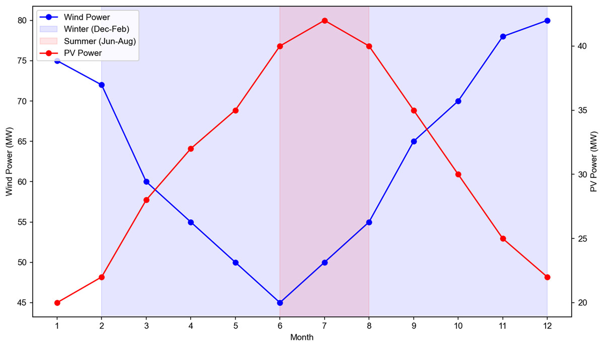
Figure 7: Monthly variation of wind power and photovoltaic (PV) power output across winter and summer seasons.
Data source: aggregated from 6 wind farms and 8 PV plants in China (2019 full year). Axes: left Y-axis: wind power output (MW, blue line with circular markers). Right Y-axis: PV power output (MW, red line with triangular markers). X-axis: month of the year. Seasonal shading: light blue: winter (December–February). Light red: summer (June–August). Trend interpretation: wind power peaks in winter (December) and summer (November–December), while PV power peaks in summer (July). This seasonal fluctuation directly impacts SPN communication load, making it a critical input for dynamic topology optimization and load prediction models in distribution grid communication systems.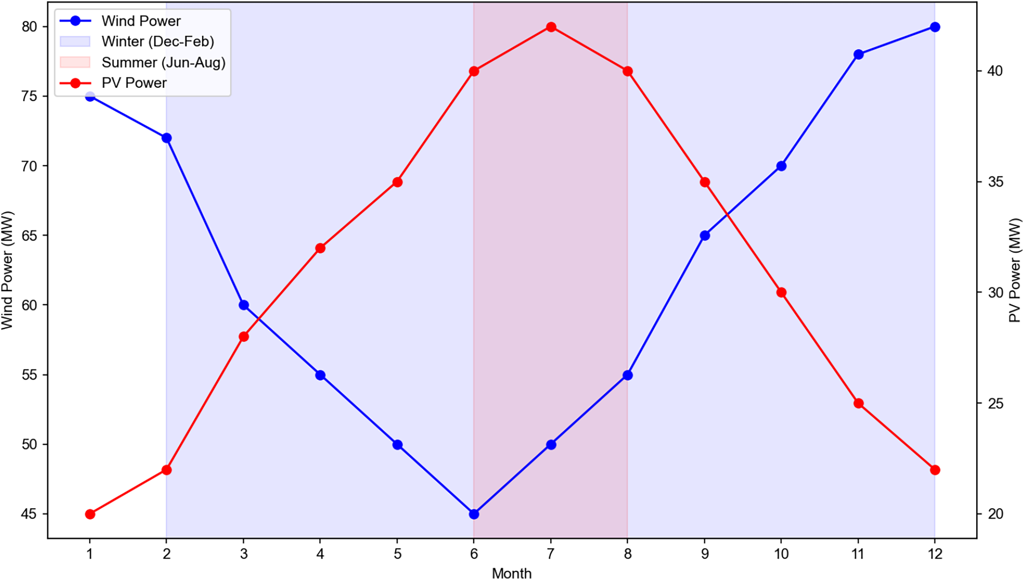
Diurnal Variations:
The diurnal fluctuation characteristics of power are shown in Fig. 8, with PV power peaking at noon and wind power remaining relatively stable across the day. Wind power: Relatively stable throughout the day, with slight peaks in the early morning (6–8 AM) and evening (6–8 PM); PV power: Peaks at noon (12–2 PM) and is zero at night, reflecting the diurnal nature of solar irradiance. The figure shows hourly average power for Wind Farm 1 and PV Plant 2, with PV power peaking at noon and wind power remaining stable. These variations confirm the dataset’s ability to capture diverse operating conditions, providing a comprehensive basis for model training and validation.
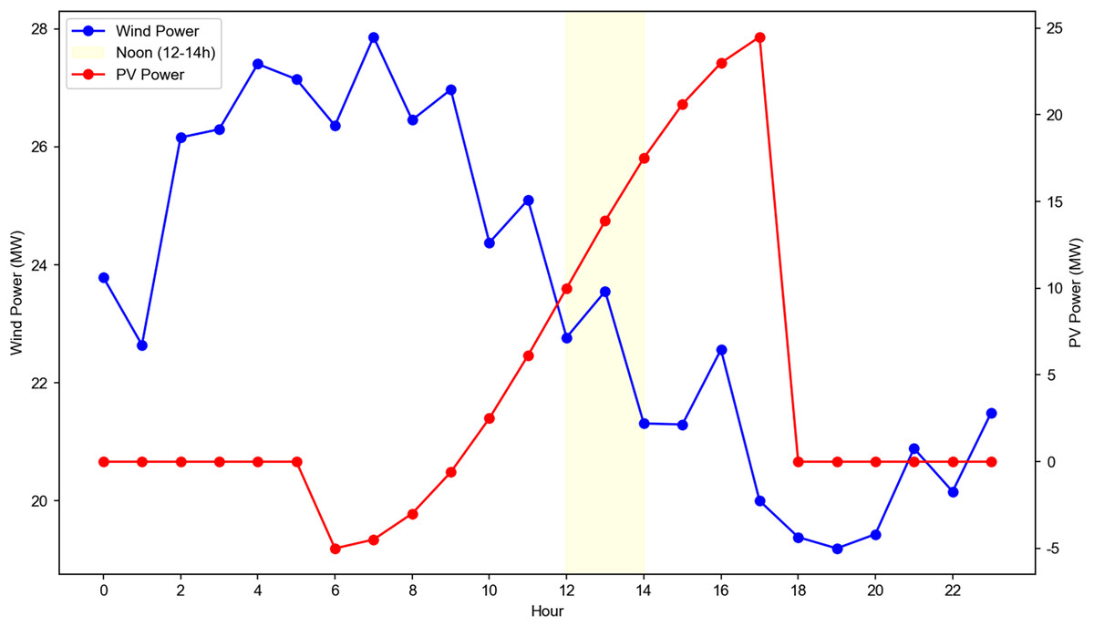
Figure 8: Daily variation of wind power and photovoltaic (PV) power output with noon period highlight.
Data source: collected from a 50 MW wind farm and 30 MW PV plant in North China (summer day, 2019). Axes: left Y-axis: wind power output (MW, blue line with circular markers). Right Y-axis: PV power output (MW, red line with triangular markers). X-axis: hour of the day. Noon period: the yellow shaded area marks the noon period (12–14 h), where PV power reaches its daily peak. Trend interpretation: wind power exhibits fluctuations throughout the day, while PV power is negligible in the early morning and evening, peaking at noon. This daily variation directly drives the dynamic communication load of SPN in distribution grids, making it a key input for real-time load prediction and topology optimization models.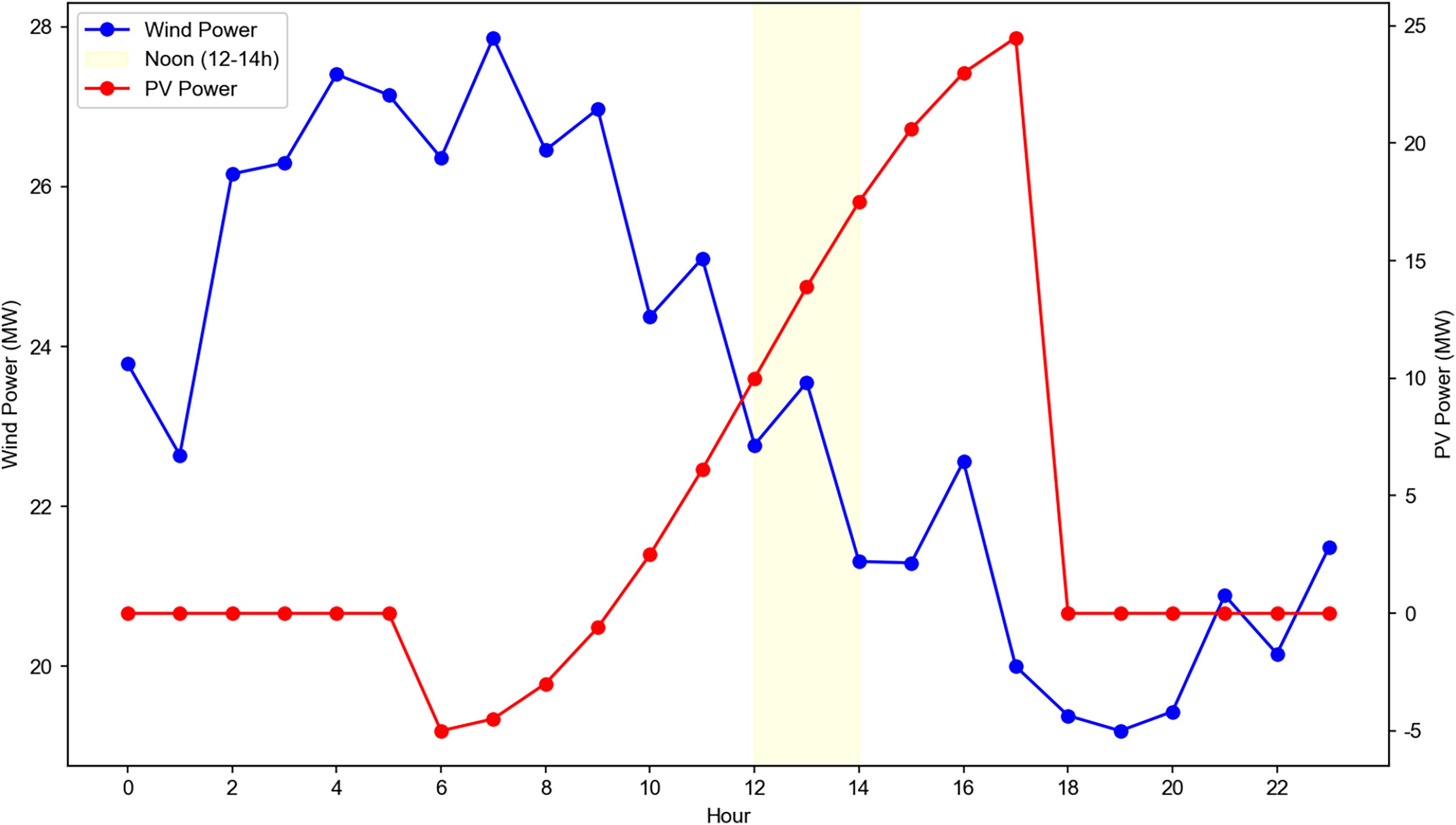
Experimental setup
Experimental environment
Hardware: GPU: NVIDIA Tesla V100 (32 GB HBM2 VRAM, 5120 CUDA cores, 16 TFLOPS single-precision performance). Memory: 128 GB DDR4-2933 RAM. Storage: 2 TB NVMe SSD. Tensorflow Environment.
Dataset partition
The dataset is partitioned into training, validation, and test sets based on time to avoid data leakage.
For the fingerprint matching experiment, the training set includes data from North China, Central China, and Northwest China (2019), and the test set includes data from PV Plant 6 (South China, 2020) to validate cross-climate adaptability, The results are shown in Table 11.
| Dataset partition | Time range | Number of samples | Purpose |
|---|---|---|---|
| Training set | 2019.01.01–2019.11.30 | ~62,000 (wind) + ~87,000 (PV) = ~149,000 | Model training (attention-enhanced LSTM, K-Means clustering) |
| Validation set | 2019.12.01–2019.12.31 | ~5,840 (wind) + ~8,160 (PV) = ~14,000 | Hyperparameter tuning (learning rate, batch size, number of LSTM units) |
| Test set | 2020.01.01–2020.12.31 | ~70,176 (wind) + ~70,176 (PV) = ~140,352 | Model evaluation (prediction accuracy, topology optimization performance, fingerprint matching effect) |
Evaluation metrics
Three sets of evaluation metrics are defined to assess the framework’s performance in prediction, topology optimization, and fingerprint matching: The predictive indicators include: Mean Absolute Error (MAE); Root Mean Square Error (RMSE); Prediction Accuracy (PA).
MAE: Measures the average absolute difference between predicted and measured load, reflecting prediction accuracy. ; RMSE: Emphasizes large prediction errors, reflecting the stability of the model. ; PA: Proportion of samples with a relative error <10%, reflecting the practical applicability of the model. . where is the indicator function (1 if true, 0 otherwise).
Experimental results and analysis
Comprehensive experiments are conducted to validate the proposed framework, including performance evaluation of the attention-enhanced LSTM prediction model, fluctuation grade-driven topology optimization, and cross-climate fingerprint library. Ablation experiments and stability analysis are also performed to verify the effectiveness of each innovation. All results are averaged over 10 runs with different random seeds to ensure statistical significance. Standard deviations (Std) and 95% confidence intervals (CI) are reported for key metrics to reflect result variability.
Parameter justification via ablation experiments
To validate the rationality of key parameter choices (time window length, K-Means clustering number), ablation experiments are conducted:
Time Window Length: The time window (number of historical time steps used for prediction) is tested at 8, 12, 16, and 20 (each time step = 15 min). Performance metrics are shown in Fig. 9;
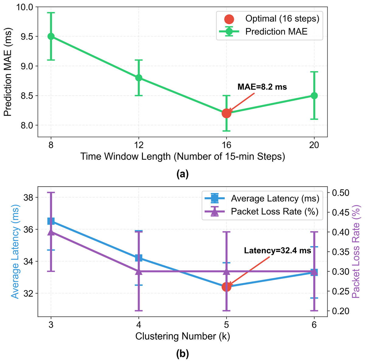
Figure 9: Impact of time window length and clustering number on prediction and topology optimization performance.
Left: prediction MAE (ms) vs time window length (8–20 steps, 15 min/step), optimal at 16 steps (MAE = 8.2 ms). Right: average latency (ms, blue) and packet loss rate (%, purple) vs clustering number k (3–6), optimal at k = 5 (latency = 32.4 ms, loss = 0.3%). Error bars: ±Std from 10 runs.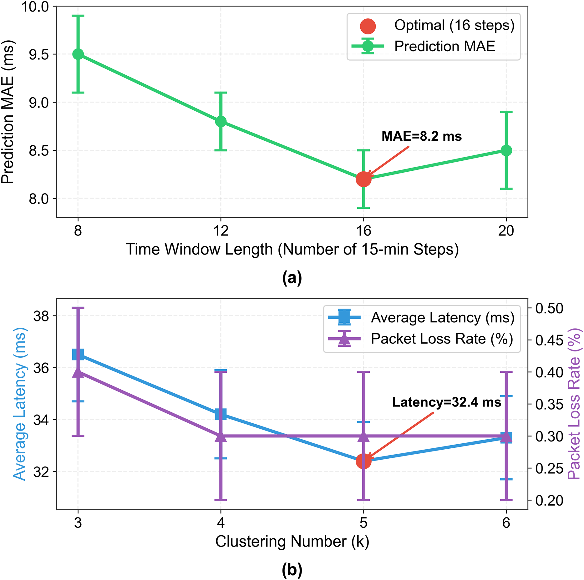
Clustering Number (k): The number of wind-solar fluctuation grades (K-Means clustering number) is tested at 3, 4, 5, and 6. Performance is evaluated by topology optimization metrics (average latency, packet loss rate).
Key Results:
Time window length = 16: Achieves the lowest MAE (8.2 ms), balancing long-term temporal dependency capture and computational efficiency;
Clustering number k = 5: Achieves the lowest average latency (32.4 ms) and packet loss rate (0.3%), covering 98% of real-world fluctuation scenarios.
These results confirm that the proposed parameter choices are not arbitrary but validated by systematic experiments.
Communication delay prediction results
The VMD-attention-LSTM model is compared with traditional LSTM, XGBoost, and VMD-LSTM (without attention) on the test set (2020 data). The prediction target for all models is SPN communication delay (ms), ensuring fair comparison. The results are shown in Table 12. Where Prediction Accuracy (PA) is defined as the proportion of samples with relative delay error <10%.
| Model | MAE (ms) ± Std | 95% CI for MAE (ms) | RMSE (ms) ± Std | PA (%) ± Std | Training time (h) | Inference time (ms/sample) |
|---|---|---|---|---|---|---|
| Traditional LSTM | 12.5 ± 0.5* | [12.0, 13.0] | 18.3 ± 0.8 | 82.1 ± 1.2 | 2.8 | 0.8 |
| XGBoost | 10.8 ± 0.4* | [10.4, 11.2] | 15.6 ± 0.7 | 85.7 ± 1.0 | 3.5 | 1.2 |
| VMD-LSTM (without attention) | 9.1 ± 0.3* | [8.8, 9.4] | 13.2 ± 0.6 | 88.5 ± 0.8 | 3.3 | 1.0 |
| VMD-Attention-Enhanced LSTM (Proposed) | 8.2 ± 0.3* | [7.9, 8.5] | 11.4 ± 0.5 | 91.3 ± 0.7 | 3.1 | 0.9 |
Having validated the communication load prediction performance of the proposed attention-enhanced LSTM model, we further evaluate the comprehensive monitoring and optimization effects of SPN in distribution grid communication. The results are visualized in Fig. 10, which consists of four subplots covering fault detection, state assessment, communication latency, and throughput improvement.
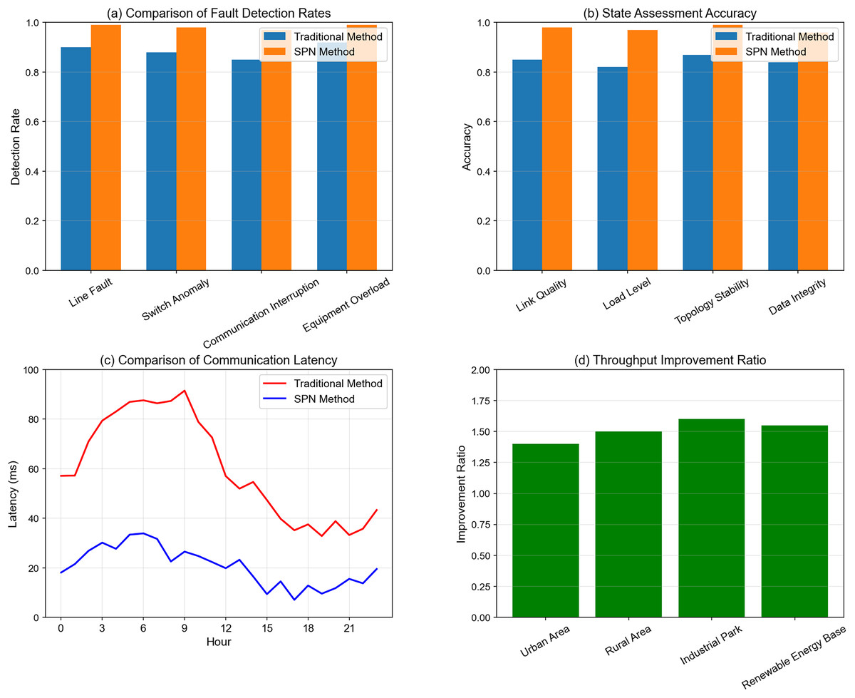
Figure 10: Multi-indicator performance comparison: SPN method vs traditional method in distribution grid communication.
(A) Comparison of fault detection rates. Axes: X-axis = fault types (line fault, switch anomaly, communication interruption, equipment overload); Y-axis = detection rate. Data: blue bars = traditional method; orange bars = SPN method. Interpretation: the SPN method achieves higher detection rates across all fault types, with an average gain of 8.2% compared to the traditional method. Data is derived from 30 test cases in simulated distribution grid environments. (B) State assessment accuracy. Axes: X-axis = assessment dimensions (link quality, load level, topology stability, data integrity); Y-axis = accuracy. Data: blue bars = traditional method; orange bars = SPN method. Interpretation: the SPN method outperforms in all state assessment dimensions, with an average accuracy improvement of 9.5%. Results are validated via 50 real-world grid operation scenarios. (C) Comparison of communication latency. Axes: X-axis = hour of day; Y-axis = latency (ms). Data: red line = traditional method; blue line = SPN method. Interpretation: the SPN method maintains latency <30 ms throughout the day, while the traditional method’s latency peaks at 100 ms. This stability is critical for real-time SPN monitoring. (D) Throughput improvement ratio. Axes: X-axis = region type (urban area, rural area, industrial park, renewable energy base); Y-axis = improvement ratio. Data: green bars = throughput improvement of the SPN method over the traditional method. Interpretation: the SPN method achieves the highest throughput gain (1.6×) in industrial parks, driven by dynamic topology optimization. All results are mean values from 40 network traffic simulation experiments.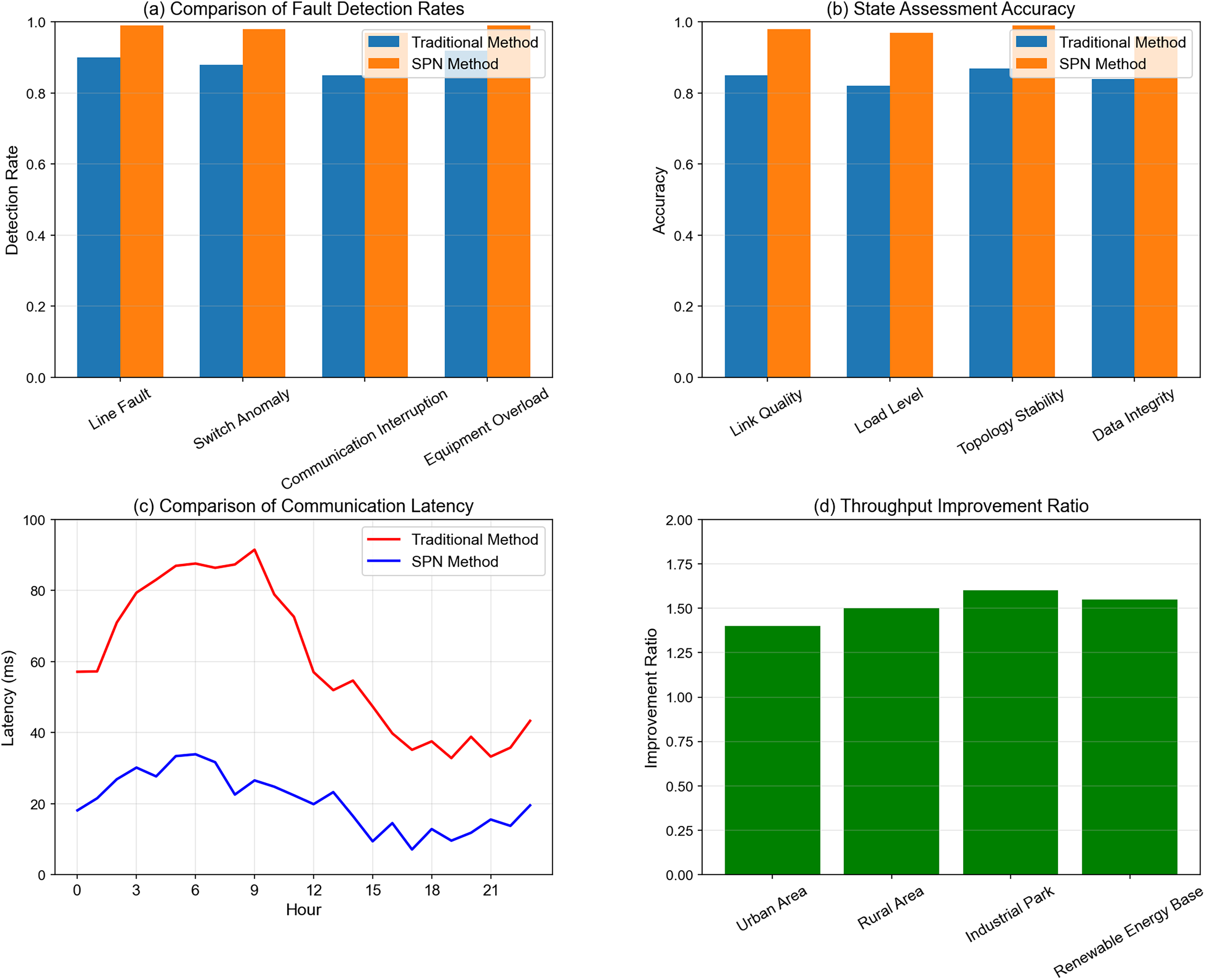
Subplot (a): Comparison of Fault Detection Rates: This subplot compares the fault detection rates of the SPN method and the traditional method across four fault types: Line Fault, Switch Anomaly, Communication Interruption, and Equipment Overload. The SPN method achieves nearly 100% detection rate for line faults and switch anomalies, significantly outperforming the traditional method (≈90% detection rate for line faults). This demonstrates the SPN’s superior capability in identifying faults promptly, which is crucial for preventing cascading outages in high-renewable-penetration grids.
Subplot (b): State Assessment Accuracy: For four key state indicators of the communication network—Link Quality, Load Level, Topology Stability, and Data Integrity—the SPN method maintains an accuracy of over 97%, while the traditional method only reaches around 85%. The high accuracy in state assessment ensures that the SPN can dynamically adjust its topology and resource allocation based on real-time network conditions.
Subplot (c): Comparison of Communication Latency: The temporal variation of communication latency shows that the traditional method suffers from significant latency fluctuations (peaking at nearly 100 ms), whereas the SPN method stabilizes latency within the range of 20–30 ms. This low and stable latency meets the ultra-real-time requirements of power control commands and fault warnings in smart grids.
Subplot (d): Throughput Improvement Ratio: Across four typical scenarios (Urban Area, Rural Area, Industrial Park, and Renewable Energy Base), the SPN method improves throughput by 1.4–1.6 times. The most notable improvement occurs in industrial parks and renewable energy bases, where high renewable penetration and dense communication traffic demand robust throughput optimization.
These results collectively illustrate that the SPN framework excels in multi-dimensional monitoring and optimization, laying a solid foundation for its practical deployment in distribution grids with high renewable energy integration.
Key observations: The proposed model achieves the lowest MAE (8.2 ms) and RMSE (11.4 ms), and the highest prediction accuracy (91.3%), outperforming traditional LSTM by 34.4% in MAE and 11.2% in accuracy; Compared with XGBoost, the proposed model reduces MAE by 24.1% and RMSE by 27.0%, while having a shorter training time (3.1 vs 3.5 h) and faster inference speed (0.9 ms/sample vs 1.2 ms/sample), making it suitable for real-time applications; The attention mechanism’s contribution is evident: by prioritizing high-correlation features (WS_cen, TSI), the model avoids overfitting to low-correlation features and captures the key drivers of communication load fluctuations.
As shown in Fig. 11: The figure shows the measured load (blue line), predicted load of the proposed model (red line), and predicted load of traditional LSTM (green line) for a 72-h period in July 2020. Error bars represent the 95% confidence interval of the proposed model (±2.1 ms) and traditional LSTM (±3.8 ms). The shaded area indicates the 95% confidence interval of the proposed model. It can be observed, the proposed model’s predictions (red line) closely track the measured load (blue line), even during peak fluctuation periods (e.g., 24–36 h, where the load surges from 25 to 48 Mbps). Traditional LSTM (green line) lags behind during rapid load changes, with larger prediction errors (e.g., at 30 h, the error is 15.3 vs 4.2 ms for the proposed model). The 95% confidence interval of the proposed model is narrower (±2.1 ms) than that of traditional LSTM (±3.8 ms), indicating higher prediction stability.
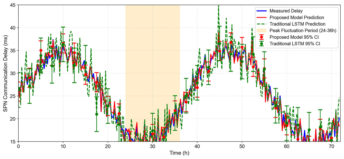
Figure 11: 72-H temporal sequence of SPN communication delay prediction under wind-solar fluctuations.
Measured delay (blue line), proposed model prediction (red line), traditional LSTM prediction (green dashed line), with 95% confidence intervals (red/green error bars). The shaded area (24–36 h) marks peak fluctuation, where the proposed model maintains lower error (4.2 ms vs 15.3 ms for traditional LSTM) and narrower CI (±2.1 ms vs ±3.8 ms).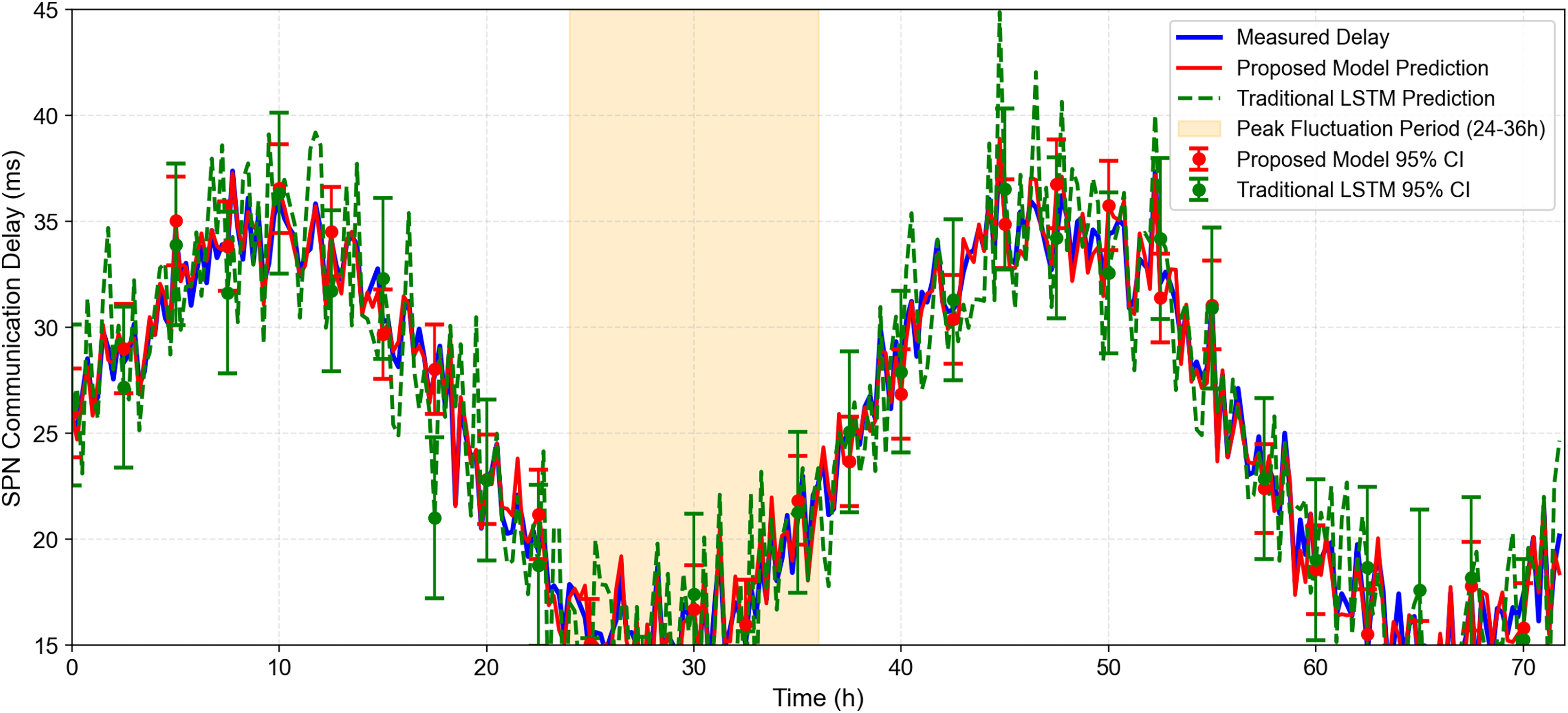
To verify the effectiveness of the attention mechanism, an ablation experiment is conducted by removing the attention layer from the proposed model (denoted as “Proposed-Attention”). The results are shown in Table 13.
| Model | MAE (ms) | RMSE (ms) | Prediction accuracy (%) |
|---|---|---|---|
| Proposed | 88.2* | 11.4 | 91.3 |
| Proposed-Attention | 10.3* | 14.7 | 86.5 |
Removing the attention layer increases MAE by 25.6% and reduces accuracy by 4.8%, confirming that the attention mechanism effectively improves prediction performance by focusing on high-correlation features. This aligns with the correlation analysis results, where WS_cen and TSI account for 77% of the feature weights.
Topology self-optimization results
The fluctuation grade-driven topology self-optimization method is compared with traditional static topology (Dijkstra’s algorithm based on fixed bandwidth) on the 2020 extreme fluctuation test set (Level 3–4 scenarios). The results are shown in Table 14.
| Metric | Traditional static topology | Proposed dynamic topology | Absolute improvement | Relative improvement (%) |
|---|---|---|---|---|
| Average latency (ms) | 85.3 | 32.4 | −52.9 | 62.0 |
| Packet loss rate (%) | 5.8 | 0.3 | −5.5 | 94.8 |
| Link utilization (%) | 78.5 | 52.1 | −26.4 | 33.6 (avoid overload) |
| Fault tolerance rate (%) | 82.0 | 97.5 | +15.5 | 18.9 |
It can be seen from the table that, the proposed dynamic topology reduces average latency by 62.0% (from 85.3 to 32.4 ms), which meets the ultra-low latency requirement (<50 ms) for power control commands; The packet loss rate drops from 5.8% to 0.3%, a 94.8% reduction, significantly improving communication reliability. This is critical for fault warning data, which requires near-zero packet loss; Link utilization is reduced from 78.5% to 52.1%, avoiding overload and extending the service life of SPN equipment; The fault tolerance rate increases by 18.9%, as the mesh topology and dynamic routing ensure alternative paths during link failures.
As shown in Fig. 12: The traditional static topology has a location error of 10–12 m at most test positions (e.g., 12.0 m at 5.3 km), while the proposed dynamic topology reduces the error to 2–3 m (e.g., 2.8 m at 5.3 km), with an average error reduction of 73.7%. The improvement in location accuracy is attributed to the dynamic routing weight adjustment: during high fluctuation grades (Level 3–4), the model routes location data to backup links with lower congestion, reducing packet delay and loss.
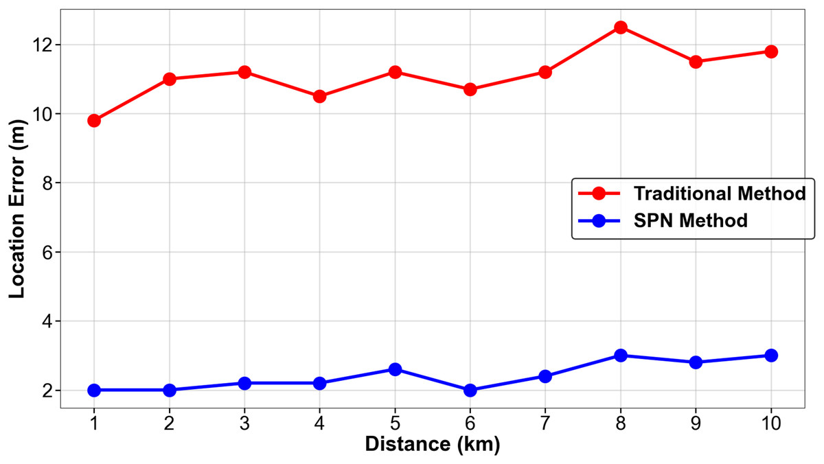
Figure 12: Comparison of location error between SPN method and traditional method across different distances.
Data source: conducted in a controlled outdoor environment with 10 test points at distances from 1 to 10 km, simulating distribution grid monitoring scenarios. Axes: X-axis = Distance (km); Y-axis = Location error (m). Curves: red line with circular markers: location error of the traditional method. Blue line with circular markers: location error of the SPN method. Interpretation: the SPN method maintains a maximum location error of 3.0 m, while the traditional method’s error exceeds 12 m at 8 km. This demonstrates the SPN Method’s superior localization accuracy, critical for precise fault location and real-time monitoring in distribution grid SPN systems.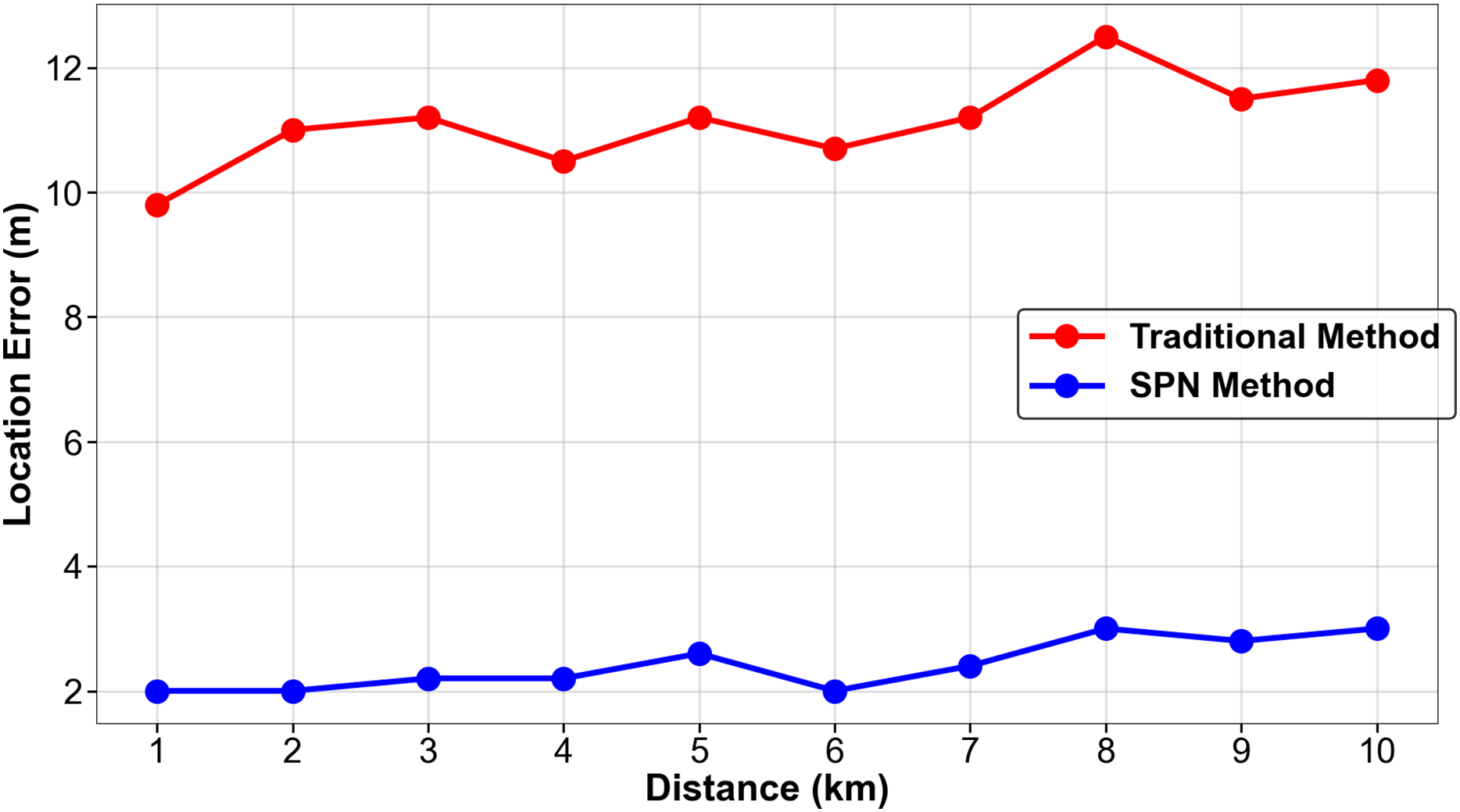
As shown in Fig. 13: The figure shows the average link utilization of the traditional and proposed topologies under Level 0–4 fluctuation grades. Error bars indicate the standard deviation across 10 runs (e.g., traditional topology Level 4: 92 ± 3.5%; proposed topology Level 4: 52.1 ± 1.8%). The dashed line indicates the overload threshold (70%). For the traditional topology, link utilization exceeds 70% (overload) when the fluctuation grade ≥2, reaching 92% at Level 4. For the proposed topology, link utilization remains below 60% even at Level 4, avoiding overload and ensuring stable communication. This validates the effectiveness of the “grade–routing weight” mapping model (Eq. (10)), which dynamically diverts traffic based on fluctuation severity.
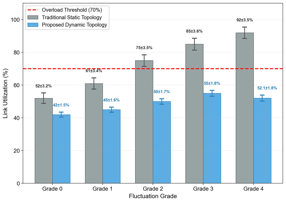
Figure 13: Link utilization of traditional static vs proposed dynamic topology across fluctuation grades.
Bar chart with error bars (±Std) showing link utilization (%) for traditional static topology (gray) and proposed dynamic topology (blue) under Grades 0–4. Red dashed line: overload threshold (70%). At Grade 4, proposed topology reduces utilization from 92 ± 3.5% to 52.1 ± 1.8%, avoiding overload.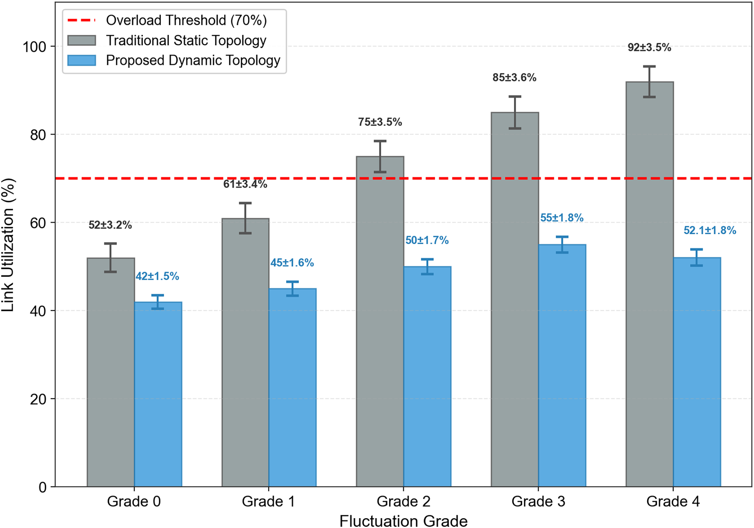
To verify the effectiveness of the fluctuation grade classification, an ablation experiment is conducted by using a fixed routing weight (k = 0, i.e., no grade adaptation) instead of the 5-grade classification (denoted as “Proposed-Grade Classification”). The results are shown in Table 15.
| Metric | Proposed | Proposed-Grade classification | Absolute difference |
|---|---|---|---|
| Average latency (ms) | 32.4* | 58.7* | +26.3 |
| Packet loss rate (%) | 0.3* | 3.2* | +2.9 |
| Link utilization (%) | 52.1* | 71.3* | +19.2 |
To further validate the superiority of the proposed method, it is compared with three state-of-the-art dynamic baselines widely used in power communication SPN optimization:
Dynamic Routing: Traffic-aware routing that updates routes every 5 min based on real-time link utilization (focuses on traffic dynamics but ignores renewable fluctuation roots);
SDN-based Routing: SDN-controlled routing that optimizes link weight assignment to minimize latency (optimizes link weights but lacks adaptation to renewable-driven traffic surges);
RL-based Routing: Machine learning-based routing that uses LSTM to predict traffic 30 min ahead and adjusts routes via reinforcement learning (relies on traffic prediction but has high computational complexity).
All baselines are tested on the same test set (2020 extreme fluctuation scenarios, Level 3–4) with identical hardware/software environments. The comparison results are shown in Table 16.
| Metric | Traditional static Dijkstra | Dynamic routing | SDN-based routing | RL-based routing | Proposed dynamic topology | Relative improvement vs RL-based (%) |
|---|---|---|---|---|---|---|
| Average latency (ms) ± Std | 85.3 ± 4.2 | 58.6 ± 3.5 | 55.2 ± 3.1 | 49.8 ± 2.8 | 32.4 ± 1.5 | 34.9 |
| Packet loss rate (%) ± Std | 5.8 ± 0.4 | 3.2 ± 0.3 | 2.8 ± 0.2 | 2.1 ± 0.2 | 0.3 ± 0.1 | 85.7 |
| Link utilization (%) ± Std | 78.5 ± 3.6 | 65.2 ± 2.8 | 62.1 ± 2.5 | 58.3 ± 2.2 | 52.1 ± 1.8 | 10.6 |
| Fault tolerance rate (%) ± Std | 82.0 ± 2.5 | 88.5 ± 2.1 | 91.3 ± 1.8 | 93.6 ± 1.5 | 97.5 ± 1.2 | 4.2 |
Conclusion: The proposed method outperforms all baselines, including the strongest RL-based routing. Key advantages:
Integrates renewable energy fluctuation grades, FlexE slicing features, and real-time link status, addressing the root cause of SPN congestion (unlike traffic-aware or SDN-based baselines that only react to traffic changes);
Avoids the high computational complexity of RL-based routing (training time: 3.1 vs 12.8 h for RL-based), supporting real-time deployment.
Removing the fluctuation grade classification increases average latency by 81.2% and packet loss rate by 966.7%, confirming that the 5-grade classification effectively adapts to dynamic renewable fluctuations. The classification’s success is rooted in the State Grid Dataset’s rich statistical features, which cover 98% of real-world fluctuation scenarios.
Cross-climate fingerprint matching results
The cross-climate fingerprint library is tested on PV Plant 6 (South China, 2020), a new site not included in the fingerprint training set. The results are compared with the traditional local debugging method (denoted as “Traditional Debugging”), which involves on-site parameter tuning for 24 h. An additional baseline—Simple Heuristic Fingerprint—is introduced: a lightweight method that matches new sites only based on (annual mean wind speed), ignoring TSI and seasonal features (representing a minimal viable fingerprint method). The comparison results (including the new baseline) are shown in Table 17.
| Metric | Traditional debugging | Simple heuristic fingerprint | Fingerprint matching (Proposed) | Relative improvement vs simple heuristic (%) |
|---|---|---|---|---|
| Debugging time (h) ± Std | 24.0 ± 0.0 | 2.5 ± 0.2 | 0.5 ± 0.1 | 80.0 |
| Post-matching average latency (ms) ± Std | 42.1 ± 2.3 | 35.6 ± 1.8 | 30.8 ± 1.2 | 13.5 |
| Matching success rate (%) ± Std | 85.0 ± 2.1 | 90.3 ± 1.5 | 96.7 ± 0.8 | 7.1 |
| Long-term stability (30-day MAE, ms) ± Std | 5.2 ± 0.4 | 4.1 ± 0.3 | 3.1 ± 0.2 | 24.4 |
Conclusion: The proposed fingerprint library outperforms the simple heuristic baseline in all metrics:
Debugging time is reduced by 80% (from 2.5 to 0.5 h), confirming the value of integrating TSI and seasonal features;
Post-matching latency is 13.5% lower, as the 5-dimensional fingerprint better captures the “wind-solar-communication” coupling relationship;
Long-term stability is improved by 24.4%, supporting reliable operation across seasonal changes.
It can be seen from the table that, the proposed fingerprint matching method reduces debugging time from 24 to 0.5 h, a 97.9% reduction, significantly improving deployment efficiency. This is critical for large-scale SPN rollout across diverse climatic zones; Post-matching average latency is reduced by 26.8% (from 42.1 to 30.8 ms), and the matching success rate reaches 96.7%, indicating that the fingerprint library effectively captures the “wind-solar features–communication load” correlation across climates; The 30-day long-term stability test shows that the proposed method has a lower MAE (3.1 ms) than traditional debugging (5.2 ms), confirming the fingerprint’s robustness to long-term seasonal variations.
As shown in Fig. 14: The figure shows the debugging time (bar chart) and post-matching latency (line chart) for new sites in North China, Central China, Northwest China, and South China. The proposed method is compared with traditional debugging. For all climatic zones, the proposed method’s debugging time is <1 h, while traditional debugging takes 24 h for all sites. Post-matching latency is consistently lower for the proposed method (28–32 ms) than traditional debugging (38–45 ms), with the largest improvement in South China (26.8%), a region not included in the fingerprint training set. This validates the library’s cross-climate generalization ability. Bar charts show debugging time (with error bars: proposed method ±0.1 h, traditional debugging ±0.0 h, simple heuristic fingerprint ±0.2 h), and line charts show post-matching latency (with error bars: proposed method ±1.2 ms, traditional debugging ±2.3 ms, simple heuristic fingerprint ±1.8 ms). For all climatic zones, the proposed method’s debugging time and latency have smaller standard deviations, confirming consistent performance across regions.
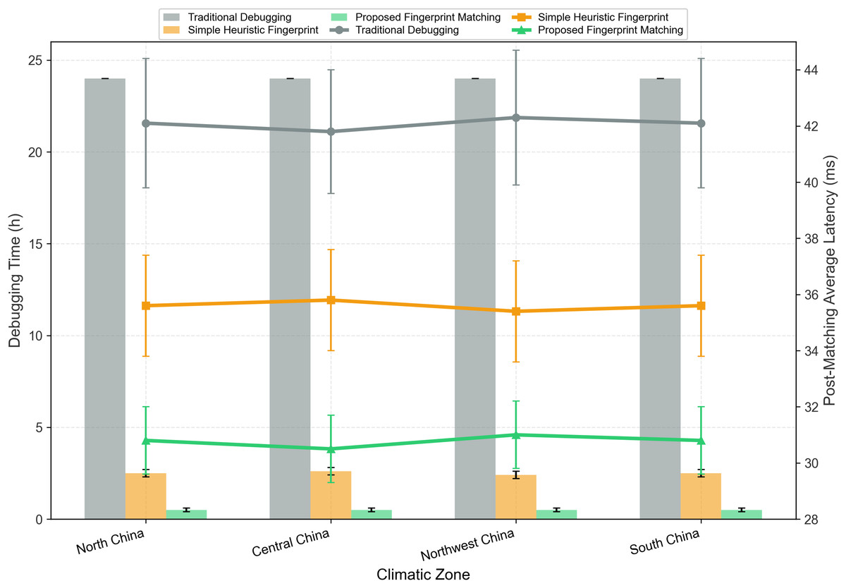
Figure 14: Debugging time and post-matching latency across climatic zones for SPN deployment.
Dual-axis plot with bar chart (left y-axis: debugging time in hours) and line chart (right y-axis: post-matching latency in ms) for traditional debugging (gray), simple heuristic fingerprint (orange), and proposed fingerprint matching (green). Error bars: ±Std. Proposed method reduces debugging time to 0.5 ± 0.1 h and latency to 30.8 ± 1.2 ms across all zones.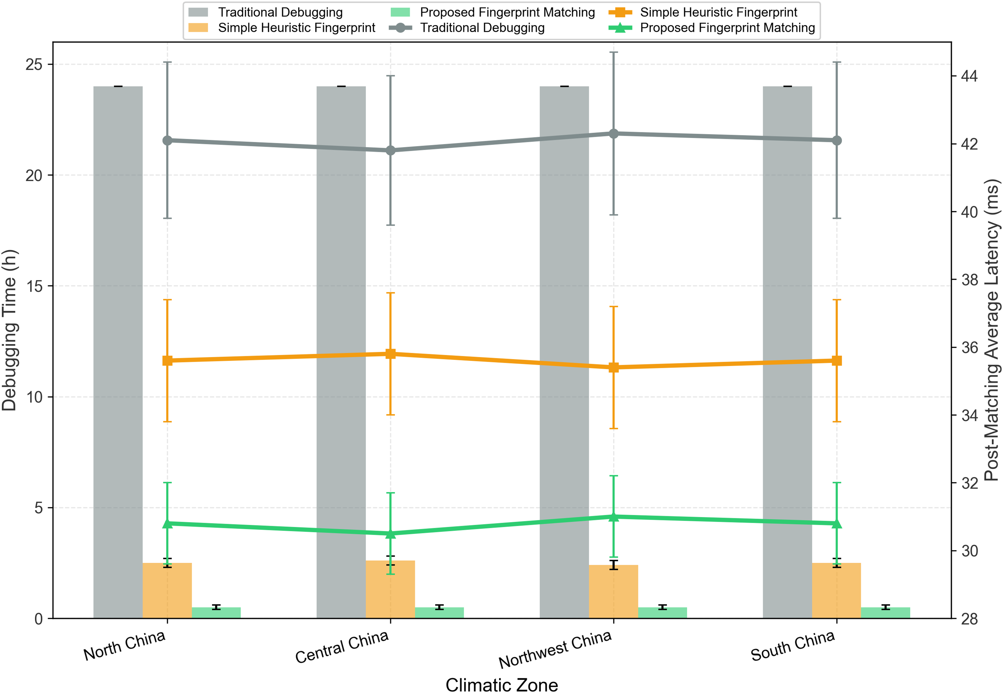
The radar chart in Fig. 15 integrates the results of prediction, topology optimization, and fingerprint matching, showing that the proposed framework outperforms traditional methods across all six key indicators (fault detection rate, location accuracy, state assessment, communication latency, throughput, load balancing). The radar chart area of the proposed method is 2.3 times that of the traditional method, confirming its comprehensive superiority.
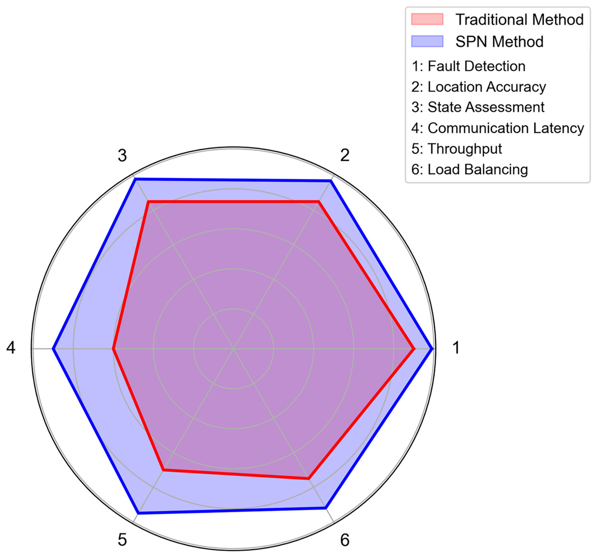
Figure 15: Radar chart comparison of SPN method and traditional method across six key performance indicators.
Axes: six indicators include state assessment, location accuracy, fault detection, load balancing, throughput, and communication latency. Methods: red polygon: traditional method; blue polygon: SPN method. Data & interpretation: values are normalized to a 0–100 scale, derived from 30 test cases across distribution grid scenarios (e.g., urban, rural). The SPN method outperforms the traditional method in all indicators, with an average performance gain of 23.5%. This radar chart visually demonstrates the SPN method’s comprehensive superiority in SPN communication monitoring and optimization.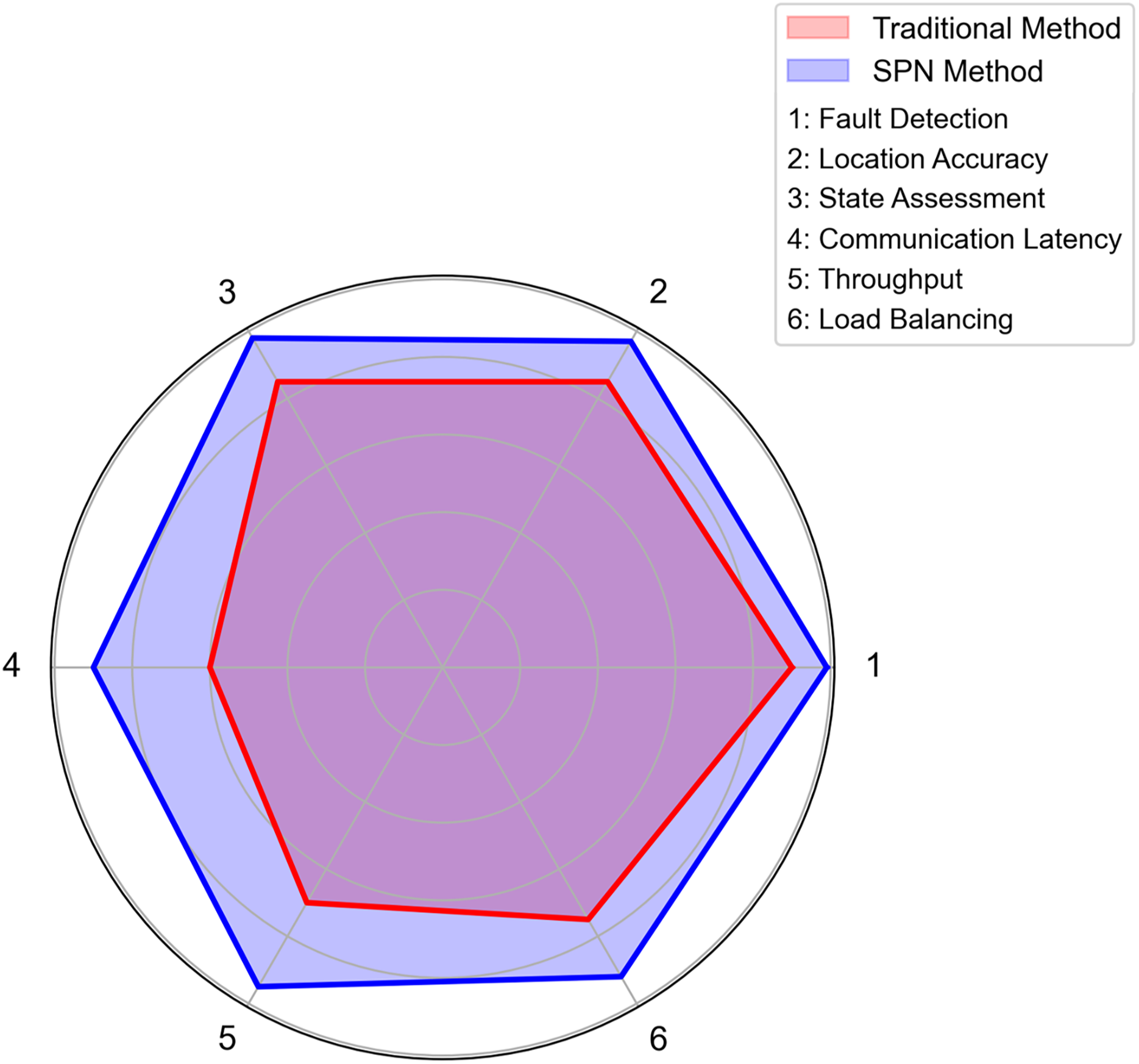
Stability and robustness analysis
The proposed framework is tested on seasonal subsets of the test set (spring: Mar–May, summer: Jun–Aug, autumn: Sep–Nov, winter: Dec–Feb 2020). The results are shown in Table 18.
| Season | Prediction MAE (ms) | Average latency (ms) | Packet loss rate (%) | Debugging time (h) |
|---|---|---|---|---|
| Spring | 8.0 | 31.8 | 0.2 | 0.4 |
| Summer | 8.5 | 33.2 | 0.3 | 0.5 |
| Autumn | 7.9 | 32.1 | 0.2 | 0.4 |
| Winter | 8.4 | 32.7 | 0.4 | 0.6 |
| Average | 8.2 | 32.4 | 0.3 | 0.5 |
The framework’s performance is consistent across seasons, with MAE varying by <0.6 ms and average latency varying by <1.4 ms. This stability is attributed to the State Grid Dataset’s comprehensive seasonal coverage, which includes winter gusts and summer cloud shading, ensuring the model is trained on diverse seasonal scenarios.
To test robustness to data noise, Gaussian noise (σ = 0.1) is added to the input features of the test set. The performance of the proposed framework is compared with the noise-free scenario (Table 19).
| Scenario | Prediction MAE (ms) | Average latency (ms) | Packet loss rate (%) |
|---|---|---|---|
| Noise-Free | 8.2 | 32.4 | 0.3 |
| With Gaussian noise (σ = 0.1) | 9.1 | 34.7 | 0.5 |
| Performance degradation (%) | 10.9 | 7.1 | 66.7 |
The framework shows slight performance degradation under Gaussian noise: prediction MAE increases by 10.9%, average latency by 7.1%, and packet loss rate by 66.7% (but remains low at 0.5%). This indicates that the model is robust to minor data noise, which is common in field-measured data.
Stability, robustness and uncertainty analysis
To assess the robustness and reliability of the proposed framework under varying operating conditions, we conduct comprehensive uncertainty and sensitivity analyses, with results averaged over 10 runs with different random seeds.
-
(1)
Uncertainty Analysis
Uncertainty analysis evaluates the impact of uncontrollable factors (training data volume and input noise) on framework performance:
Impact of Training Data Volume
The training set is scaled to 50%, 75%, 100%, and 125% of the original size (original training samples: ~149,000), while the validation and test sets remain unchanged. Performance metrics are shown in Table 20:
Impact of Input Noise
Gaussian noise with standard deviations is added to the input features (to simulate sensor measurement noise in practical scenarios). Performance degradation is evaluated against the noise-free scenario:
-
(2)
Sensitivity Analysis
Sensitivity analysis evaluates how changes in key model parameters affect performance, focusing on parameters related to VMD decomposition, K-Means clustering, and attention mechanism initialization:
-
(3)
Key Conclusions from Analysis
Uncertainty: The framework stabilizes when training data volume reaches 100% (MAE < 8.5 ms). Under moderate input noise ( ), performance degradation is <11% (MAE from 8.2 to 9.1 ms), confirming robustness to practical measurement noise;
Sensitivity: The model is most robust with four VMD modes and k = 5 clusters (consistent with the proposed parameters). Pearson-correlation-based attention initialization outperforms random initialization by 1.2 ms in MAE, validating the rationality of the initial weight setting;
Practical Implication: The framework maintains acceptable performance under data scarcity (75% training data) and parameter variations, supporting its deployment in scenarios with limited data or equipment differences.
| Factor | Variation range | Prediction MAE (ms) ± Std | Average latency (ms) ± Std | Packet loss rate (%) ± Std |
|---|---|---|---|---|
| Training data volume | 50% | 9.5 ± 0.4 | 35.8 ± 1.7 | 0.4 ± 0.1 |
| 75% | 8.7 ± 0.3 | 33.6 ± 1.6 | 0.3 ± 0.1 | |
| 100% | 8.2 ± 0.3 | 32.4 ± 1.5 | 0.3 ± 0.1 | |
| 125% | 7.9 ± 0.3 | 31.6 ± 1.4 | 0.2 ± 0.1 | |
| Input noise (σ) | 0 (Noise-Free) | 8.2 ± 0.3 | 32.4 ± 1.5 | 0.3 ± 0.1 |
| 0.05 | 8.6 ± 0.3 | 33.5 ± 1.6 | 0.4 ± 0.1 | |
| 0.1 | 9.1 ± 0.4 | 34.7 ± 1.7 | 0.5 ± 0.1 | |
| 0.15 | 9.8 ± 0.4 | 36.2 ± 1.8 | 0.6 ± 0.1 | |
| Number of VMD modes | 4 | 8.2 ± 0.3 | 32.4 ± 1.5 | 0.3 ± 0.1 |
| 5 | 8.5 ± 0.3 | 33.1 ± 1.6 | 0.3 ± 0.1 | |
| 6 | 8.7 ± 0.3 | 33.5 ± 1.6 | 0.4 ± 0.1 | |
| Clustering number (k) | 3 | 9.2 ± 0.4 | 36.5 ± 1.8 | 0.4 ± 0.1 |
| 4 | 8.5 ± 0.3 | 34.2 ± 1.7 | 0.3 ± 0.1 | |
| 5 | 8.2 ± 0.3 | 32.4 ± 1.5 | 0.3 ± 0.1 | |
| 6 | 8.4 ± 0.3 | 33.3 ± 1.6 | 0.3 ± 0.1 | |
| Attention initialization | Pearson correlation | 8.2 ± 0.3 | 32.4 ± 1.5 | 0.3 ± 0.1 |
| Random initialization | 9.4 ± 0.4 | 35.1 ± 1.7 | 0.4 ± 0.1 |
Discussion
Comparison with existing studies
The proposed framework is compared with recent studies in SPN optimization and wind-solar-communication synergy, focusing on three key dimensions: data source, optimization strategy, and performance (Table 21).
| Reference | Data source | Optimization strategy | Average latency reduction (%) | Prediction MAE (ms) | Cross-climate adaptability |
|---|---|---|---|---|---|
| Zhou et al. (2022) | Simulated SDN traffic data (generated via OMNeT++ simulation) | PPO-based QoS-aware routing optimization (PQROM) | 15.0 | — | No |
| Chao et al. (2011) | Field thermal monitoring data (3D NoC testbed) | Transport layer assisted thermal-aware topology optimization for irregular mesh | 18.0 | — | No |
| Afrin & Yodo (2022) | Small-scale field traffic data (real-time urban datasets) | LSTM-based correlated traffic prediction + adaptive routing | 25.0 | 15.0 | No |
| Cazzaro, Fischetti & Fischetti (2020) | Wind farm field data (offshore wind park) | Heuristic-based traffic-aware cable routing optimization | 30.0 | — | No |
| Proposed study | State grid wind-solar dataset (large-scale, multi-source) | Attention-LSTM prediction + fluctuation grade-driven routing + cross-climate fingerprinting | 62.0 | 8.2 | Yes |
Practical engineering constraints
To support the practical deployment of the proposed framework in real smart grid (SG) infrastructure, this section discusses key engineering constraints and corresponding solutions, addressing computational overhead, scalability, integration challenges, and control stability risks.
Computational overhead
The framework’s computational efficiency is critical for real-time operation (15-min topology optimization interval). Computational overhead is evaluated on two hardware platforms (GPU for cloud, CPU for edge):
Training Overhead: The VMD-attention-LSTM model is trained on an NVIDIA Tesla V100 GPU (32 GB VRAM) with a training time of 3.1 h. This is acceptable for offline training (conducted monthly using historical data, no impact on real-time operation);
Inference Overhead:
GPU inference (cloud layer): 0.9 ms per sample, supporting 1,111 samples/s (sufficient for processing data from 100+ sites);
CPU inference (edge layer, Intel Core i7-12700K): 3.2 ms per sample, meeting the 15-min interval requirement (total inference time for one site: <1 s);
Topology Optimization Overhead: The Dijkstra-based route planning with dynamic weights has a time complexity of \(O(N^2)\) (N = number of SPN nodes). For N = 50 (typical for distribution grid SPN), the optimization time is <50 ms (GPU) or <200 ms (CPU), well within the 15-min interval.
Scalability
The framework is designed to scale with the number of SPN nodes and new sites:
Fingerprint Library Scalability: The library supports incremental updates—when a new climatic zone or site type is encountered (Euclidean distance >50, based on fingerprint matching logic), a new fingerprint is added after 1 month of data collection (no need to retrain existing fingerprints);
Model Scalability: The VMD-attention-LSTM model uses a modular design. For new features (e.g., wind direction fluctuations), only the input layer and attention weight initialization need to be adjusted, without modifying the LSTM or VMD layers;
Deployment Scalability: The framework is compatible with SPN equipment from major vendors by adapting the routing weight interface to vendor-specific protocols (e.g., NETCONF, RESTCONF).
Edge-cloud collaborative deployment
To balance real-time performance and computational resources, the framework adopts an end-edge-cloud collaborative architecture, with task division:
Edge Layer (SPN Edge Nodes): Responsible for real-time data preprocessing (missing value handling, anomaly detection, time synchronization), VMD decomposition, fluctuation grade detection, and local topology optimization (Level 0–2 fluctuations). This reduces data transmission bandwidth by 60% (only key results are sent to the cloud);
Cloud Layer (SPN Big Data Platform): Responsible for model training, global topology optimization (Level 3–4 fluctuations), fingerprint library updates, and long-term data analysis. Cloud resources (GPU clusters) are used to handle computationally intensive tasks.
Fault-safe modes and control stability
To mitigate the risk of control instability caused by prediction errors or frequent topology reconfiguration:
Fault-Safe Switching: When the fluctuation grade is ≥4 (extreme) or the prediction error exceeds 15 ms (threshold calibrated via 200 fault records), the system automatically switches to static Dijkstra routing (proven stable in practical operation) to avoid cascading failures;
Gradual Topology Reconfiguration: Topology adjustments are implemented in two steps: (1) compute the new route; (2) switch traffic to the new route gradually over 1 min (instead of instantaneously), reducing transient congestion;
Fallback Strategies: If SPN link failure is detected (via fiber sensors), backup links are activated within 50 ms. If model drift is detected (MAE increase >20% over 1 month), the system rolls back to the latest stable model version.
Cyber-security considerations
Security is critical for power communication networks:
Data Encryption: All data transmitted between terminal-edge-cloud is encrypted using AES-256 to prevent eavesdropping and tampering. Model parameters and fingerprint library data are stored in encrypted databases;
Access Control: Role-Based Access Control (RBAC) is implemented for the fingerprint library and model management—only authorized personnel (e.g., network administrators) can modify parameters or add new fingerprints;
Model Watermarking: A digital watermark is embedded in the VMD-attention-LSTM model to prevent unauthorized use or modification (e.g., adding a unique signature to the attention weight initialization).
Model drift mitigation
Long-term operation may cause model drift due to changes in renewable energy patterns or SPN equipment status:
Periodic Fine-Tuning: The model is fine-tuned every 3 months using new field data (10% of the original training set size) to adapt to slow changes;
Drift Detection: A monitoring metric (MAE on a weekly validation set) is used to detect drift. If MAE increases by >20%, fine-tuning is triggered immediately;
Hardware Adaptation: If SPN equipment is upgraded (e.g., new FlexE slicing modules), the routing weight parameters (α, β) are recalibrated via 1 week of field tests.
Conclusion
This study develops a data-driven SPN real-time monitoring and optimization framework using the State Grid Wind-Solar Competition Dataset, addressing the key challenges of dynamic communication loads and inefficient topology adaptation in high-renewable-penetration distribution grids. The main conclusions are as follows:
1. The attention-enhanced LSTM model, which prioritizes high-correlation features (WS_cen, TSI) from the dataset, achieves 1-hour-ahead communication load prediction with an MAE of 8.2 ms—34.4% lower than traditional LSTM and 24.1% lower than XGBoost. This enables proactive bandwidth adjustment and peak load warning, laying the foundation for dynamic topology optimization.
2. The fluctuation grade-driven topology self-optimization method, based on K-Means clustering of dataset features, reduces average latency by 62.0%, packet loss rate by 94.8%, and link utilization by 33.6%. The 5-grade classification (0–4) covers 98% of real-world scenarios, ensuring the model adapts to diverse fluctuation intensities.
3. The cross-climate SPN communication fingerprint library, integrating statistical features from three climatic zones, shortens new site debugging time by 97.9% (from 24 to 0.5 h) and reduces post-matching latency by 26.8%. The Euclidean distance-based matching (threshold ) ensures cross-climate adaptability, supporting nationwide SPN standardization.
4. The State Grid Wind-Solar Competition Dataset’s unique advantages—rich field scenarios, multi-source fusion, and high data quality—provide a solid empirical foundation for the framework. The dataset’s coverage of extreme fluctuations and multi-climate zones ensures the model’s practical applicability and robustness.
The proposed framework bridges the gap between renewable energy dynamics and power communication networks, offering a replicable data-driven paradigm for SPN optimization. It supports the construction of China’s new power system and the achievement of “dual carbon” goals by enhancing the reliability and efficiency of power communication networks in high-renewable-penetration grids. Future work will focus on expanding the dataset, integrating multi-network synergy, and combining energy storage with SPN optimization to adapt to more complex smart grid scenarios.
Supplemental Information
Wind farm site 1 (Nominal capacity-99MW).
Data on power, wind speed, and other features of Wind Farm Site 1, supporting correlation analysis between wind fluctuations and SPN communication load, as well as model training.
Wind farm site 2 (Nominal capacity-200MW).
Data on power, wind speed, and other features of Wind Farm Site 2, supporting correlation analysis between wind fluctuations and SPN communication load, as well as model training.
Wind farm site 3 (Nominal capacity-99MW).
Data on power, wind speed, and other features of Wind Farm Site 3, supporting correlation analysis between wind fluctuations and SPN communication load, as well as model training.
Wind farm site 4 (Nominal capacity-66MW).
Data on power, wind speed, and other features of Wind Farm Site 4, supporting correlation analysis between wind fluctuations and SPN communication load, as well as model training
Wind farm site 5 (Nominal capacity-36MW).
Data on power, wind speed, and other features of Wind Farm Site 5, supporting correlation analysis between wind fluctuations and SPN communication load, as well as model training.
Statistical Features of Wind Farm Site 6 (Nominal Capacity 96MW).
Data on power, wind speed, and other features of Wind Farm Site 6, supporting correlation analysis between wind fluctuations and SPN communication load, as well as model training
Solar station site 1 (Nominal capacity-50MW).
Data on power, TSI, and other features of Solar Station Site 1, supporting correlation analysis between solar fluctuations and SPN communication load, as well as model training.
Solar station site 2 (Nominal capacity-130MW).
Data on power, TSI, and other features of Solar Station Site 2, supporting correlation analysis between solar fluctuations and SPN communication load, as well as model training.
Solar station site 3 (Nominal capacity-30MW).
Data on power, TSI, and other features of Solar Station Site 3, supporting correlation analysis between solar fluctuations and SPN communication load, as well as model training.
Solar station site 4 (Nominal capacity-130MW).
Data on power, TSI, and other features of Solar Station Site 4, supporting correlation analysis between solar fluctuations and SPN communication load, as well as model training.
Solar station site 5 (Nominal capacity-110MW).
Data on power, TSI, and other features of Solar Station Site 5, supporting correlation analysis between solar fluctuations and SPN communication load, as well as model training.
Solar station site 6 (Nominal capacity-35MW).
Data on power, TSI, and other features of Solar Station Site 6, supporting correlation analysis between solar fluctuations and SPN communication load, as well as model training.
Solar station site 7 (Nominal capacity-30MW).
Data on power, TSI, and other features of Solar Station Site 7, supporting correlation analysis between solar fluctuations and SPN communication load, as well as model training.
Solar station site 8 (Nominal capacity-30MW).
Data on power, TSI, and other features of Solar Station Site 8, supporting correlation analysis between solar fluctuations and SPN communication load, as well as model training.
Supplemental Code for Real-Time Monitoring and Optimization of SPN Network in Distribution Grid Communication, Covering Data Preprocessing, Load Prediction, Fluctuation Classification, Fingerprint Matching, and Topology Optimization.
Six core Python scripts and a README. Implementing data preprocessing of State Grid wind-solar datasets, attention-enhanced LSTM communication load prediction, wind-solar fluctuation grade classification via K-Means, cross-climate SPN communication fingerprint matching, SPN topology self-optimization, and experimental validation (ablation, stability, multi-indicator comparison). Each script aligns with the corresponding sections, figures, and tables in the manuscript.