
Spatio temporal attention mechanism for real time cellular traffic prediction
- Published
- Accepted
- Received
- Academic Editor
- Davide Chicco
- Subject Areas
- Algorithms and Analysis of Algorithms, Artificial Intelligence, Computer Networks and Communications, Data Mining and Machine Learning, Neural Networks
- Keywords
- Hybrid attention, Spatio temporal attention, Traffic prediction, Lightweight convolution, Cellular networks
- Copyright
- © 2026 Samudrala and Senapati
- Licence
- This is an open access article distributed under the terms of the Creative Commons Attribution License, which permits unrestricted use, distribution, reproduction and adaptation in any medium and for any purpose provided that it is properly attributed. For attribution, the original author(s), title, publication source (PeerJ Computer Science) and either DOI or URL of the article must be cited.
- Cite this article
- 2026. Spatio temporal attention mechanism for real time cellular traffic prediction. PeerJ Computer Science 12:e3571 https://doi.org/10.7717/peerj-cs.3571
Abstract
Accurate prediction of cellular network traffic is a fundamental requirement for ensuring efficient network performance in the context of increasing mobile data demands. Existing models such as Convolutional Neural Network-Long Short Term Memory (CNN-LSTM), Temporal Fusion Transformer (TFT), and Reslearn often lack the capacity to capture the complex spatio and temporal patterns and variability inherent in real-world traffic, thereby limiting their effectiveness in practical deployments. This study proposes a lightweight hybrid framework incorporating a Spatio Temporal model with Attention Mechanism (STAM) to address these limitations and enhance predictive performance. The proposed model is trained on real-world cellular network data and is designed to capture both short-term fluctuations and long-term temporal dependencies. The attention mechanism embedded within the architecture allows the model to selectively focus on salient temporal features, improving its ability to learn meaningful traffic patterns while maintaining computational efficiency. Evaluation with standard metrics such as Root Mean Square Error (RMSE), Mean Absolute Error (MAE), Symmetric Mean Absolute Percentage Error (SMAPE), and R2 demonstrates improved prediction accuracy compared to traditional baseline models. The resulting predictions provide actionable insights for dynamic resource allocation and informed network planning. These capabilities support reduced latency, improved traffic distribution, and efficient bandwidth utilization, thereby contributing to enhanced Quality of Service (QoS), Spectrum Efficiency (SE), and Network Utility (NU) within next-generation cellular systems.
Introduction
With the rapid growth of digital technologies in both everyday life and industrial settings, cellular networks are facing increasingly complex demands. Modern services such as video streaming, online gaming, remote healthcare, smart transportation, and automation require networks that can deliver reliable performance despite constantly changing traffic conditions (Saad, Bennis & Chen, 2019). Recent studies emphasize the importance of attention-based and context-aware deep learning models for intelligent traffic management in 6G networks (Das et al., 2025). These growing and diverse requirements are placing significant pressure on current network systems, revealing limitations in how well they can manage fluctuating data loads. One of the major challenges in this context is the ability to accurately predict network traffic. Without dependable traffic prediction, it becomes difficult for network providers to manage resources efficiently, ensure consistent service quality, and prevent congestion. Accurate traffic prediction plays a key role in making networks more responsive in real time, improving the overall user experience, and supporting the effective use of limited infrastructure especially as we move toward more advanced, next generation network technologies.
Conventional traffic prediction has often relied on statistical models like AutoRegressive model (AR) and Auto Regressive Integrated Moving Average Model (ARIMA) (Moayedi & Masnadi-Shirazi, 2008), which use historical data to predict future trends. While effective in stable settings, these methods struggle with the non linearity, noise, and variability found in real world network traffic (Box et al., 2015). Some enhancements, such as decomposing traffic into trends and abrupt changes, have been explored but still lack adaptability and generalization. Recently, deep learning has shown promise by capturing complex temporal patterns from large datasets. However, many models face challenges in efficiently learning relevant features, resulting in limited accuracy and high computational cost barriers to real time, practical deployment. Existing spatio-temporal models like Convolutional Neural Network-Long Short Term Memory (CNN-LSTM), Gated Recurrent Unit (GRU)-based, and hybrid attention networks often achieve high accuracy but suffer from high computational overhead, limited adaptability, and weak generalization across varying traffic patterns.
To address the limitations of existing approaches, this study introduces a lightweight deep learning framework that combines a hybrid attention mechanism with Spatio Temporal model with Attention Mechanism (STAM). The proposed approach is designed for both accuracy and efficiency, capable of capturing short term variations and long term patterns in network traffic while keeping computational demands low. Its core components include an Efficient Hybrid Attention (EHA) module for improved feature extraction, Depthwise Separable Convolution (DSC) to reduce complexity, and an STAM to focus on the most relevant time and location based information. This approach is not only a technical advancement but also a response to the growing need for intelligent, adaptive network management. By enhancing prediction accuracy, the model may support more effective load balancing, dynamic bandwidth allocation, and proactive congestion control. These improvements are key to strengthening Quality of Service (QoS), Network Utility (NU), and Spectrum Efficiency (SE) like critical factors for the evolution of next generation cellular networks. The main contributions of this work are outlined below.
We propose a unified framework that efficiently learns spatial and temporal dependencies within cellular traffic data, enabling accurate real-time traffic volume prediction with reduced computational cost.
Our proposed framework incorporates an adaptive attention strategy that jointly captures spatial and temporal correlations, allowing the model to focus on the most influential regions and time intervals under dynamic network conditions.
Further we develop a lightweight feature extraction strategy that forms the architectural foundation of STAM, achieving robust predictive performance while significantly minimizing model complexity and training overhead.
The proposed model demonstrates superior performance through comprehensive experimentation, where the proposed model consistently outperforms baseline methods using key evaluation metrics such as Root Mean Square Error (RMSE), Mean Absolute Error (MAE), Symmetric Mean Absolute Percentage Error (SMAPE), and .
In the rest of this article, Related Work is reviewed in ‘Related Work’, Dataset description and data preprocessing is presented in ‘Dataset Description and Preprocessing’, Proposed Methodology is presented in ‘Proposed Methodology’, Experimental results are discussed in ‘Results and Analysis’ and finally, ‘Conclusion’ concludes this article.
Related work
In recent years, traffic forecasting has advanced from basic statistical models to deep learning approaches that handle complex spatial and temporal patterns. Early models like ARIMA and Generalized AutoRegressive Conditional Heteroskedasticity (GARCH) captured linear and seasonal trends (Zhou et al., 2005; Yu et al., 2010), but failed to represent nonlinear dynamics (Li et al., 2017). Machine learning methods such as Support Vector Regression (SVR) and Gaussian Processes addressed non-linearity but faced scalability issues on large data (Cortes & Vapnik, 1995). Deep learning models including CNN, Recurrent Neural Network (RNN), Long Short-Term Memory (LSTM), and GRU achieved better temporal learning (LeCun et al., 1998; Bai, Kolter & Koltun, 2018). The work reported in LeCun et al. (1998) demonstrated the power of convolution networks for spatial feature extraction, inspiring their use in traffic prediction. However, most models still emphasize temporal aspects and neglect spatial relationships, leading to less accurate spatio-temporal forecasting. Hybrid models, such as CNN, RNN combinations and attention integrated architectures, address this by modeling both spatial and temporal patterns. Dense CNN improve accuracy but increase computational load (Zhang et al., 2018), while Hybrid Spatio Temporal Network (HSTNet) balances efficiency with accuracy using attention and deformable convolutions (Zhang et al., 2020). Lightweight models like Fully Connected Sequential Network (FCSN) and 1 Dimensional-Convolutional Neural Network (1D-CNN) achieve lower MAE with reduced complexity and faster execution (Mohseni, Nikan & Shami, 2022). Table 1 summarizes the state-of-the-art literature and existing baseline models commonly used for comparison in spatio temporal prediction, where the notation “S” represents spatial components, “T” denotes temporal components, and “S, T” indicates the integration of both spatial and temporal components.
| Method | Dataset | S | T | S,T | Contributions | Limitations | Metrics |
|---|---|---|---|---|---|---|---|
| HA (Qiu et al., 2018) | City cellular (Azari et al., 2019) | T | Past average baseline | Ignores spatial + trends | RMSE | ||
| ARIMA (Moayedi & Masnadi-Shirazi, 2008) | City cellular (Azari et al., 2019) | T | Linear time series modeling | No spatial, non linear limits | MAE, RMSE | ||
| RNN (Qiu et al., 2018) | City cellular (Azari et al., 2019) | T | Sequential modelling | Weak long term memory | MAE, RMSE | ||
| LSTM (Wang et al., 2017) | Shanghai (Wang et al., 2015) | T | Captures long dependencies | Ignores spatial, costly | RMSE, R2 | ||
| STDenseNet (Zhang et al., 2018) | Milan (Barlacchi et al., 2015) | S | T | ST | Dense CNN fusion | Overfit, compute intensive | RMSE, MAE |
| HSTNet (Zhang et al., 2020) | Milan (Barlacchi et al., 2015) | S | T | ST | Joint spatial temporal modeling | Complex tuning needed | RMSE, MAE, R2 |
| DCGMAM (Xiao et al., 2025) | Milan (Barlacchi et al., 2015) | S | T | ST | Diffusion GRU + attention | High overhead, scaling issues | RMSE, MAE, R2 |
| STMP (Gong et al., 2025) | Shanghai, Nanjing (Wang et al., 2015; Gong et al., 2024) | S | T | ST | Cross attn + spatial encoding | Difficult on large networks | RMSE, MAE |
| TFT (Kougioumtzidis et al., 2025) | Milan (Barlacchi et al., 2015) | T | Attn based temporal learning | No spatial, memory heavy | RMSE, MAE, R2 | ||
| Proposed model (STAM) | Telecom Italia (Telecom Italia, 2015) | S | T | ST | Conv + EHA + temporal attention | Some tuning needed | RMSE, MAE, SMAPE, |
Recent innovations in attention-based models have advanced the modeling of dynamic spatial and temporal dependencies. Models like Non-Local Graph Neural Networks with Non-Local Attention Mechanism (NLG-NLAM) effectively capture evolving spatial correlations while highlighting critical temporal features (Rao et al., 2022). Lightweight techniques, such as DSC and convolution, reduce computational complexity without compromising feature quality (Howard et al., 2017). The integration of DenseNet, derived from Residual Network (ResNet), enhances feature reuse and information flow (Huang et al., 2017). Attention modules like Convolution Block Attention Module (CBAM) further improve performance by combining spatial and channel attention (Woo et al., 2018). Optimizers such as Adaptive Moment Estimation with Weight Decay (AdamW) also contribute to faster and more stable convergence (Loshchilov & Hutter, 2017). Hybrid models, including correlation-based Convolutional Long Short-Term Memory (ConvLSTM) and three-dimensional residual convolutional networks (ResConv3D), enable efficient spatio temporal learning (Ma et al., 2023; Wang & Wong, 2022). Attention-based Multi-Scale Spatial-Temporal Cross Network (Att-MCSTCNet) leverages ConvLSTM and Convolutional Gated Recurrent Unit (ConvGRU) for enhanced temporal embedding and cross-domain fusion (Zeng et al., 2021). Complete Ensemble Empirical Mode Decomposition with Adaptive Noise (CEEMDAN) based frameworks, integrating Temporal Convolutional Network (TCN), GRU, and attention, effectively capture both short and long-term patterns (Wang, Bao & Wang, 2023). Transformer-based networks, like Spatial-Temporal Decomposable Network (STD-Net), model complex spatial-temporal interactions in mobile traffic (Hu et al., 2022). Federated learning strategies have also emerged, such as the multi-objective federated traffic prediction model for vehicular networks, enabling collaborative, privacy-preserving, and context-aware traffic forecasting in intelligent transportation systems (Aalavanthar et al., 2025). Finally, Diffussion Convolutional GRU-Multi head Attention Mechanism (DCG-MAM) integrates Diffusion Convolutional GRU with Multi-Head Attention, enabling localized spatial learning and key temporal feature extraction. The Spatiotemporal Transformer Framework (STMP) model (Gong et al., 2025) integrates temporal cross-attention and hierarchical spatial encoding to jointly predict traffic and user density, effectively capturing semantic relationships and inter-station interactions. The TFT (Kougioumtzidis et al., 2025) enhances multivariate prediction through interpretable attention-based temporal fusion, showing adaptability to dynamic scenarios like next generation cellular networks. These approaches highlight the value of hybrid attention, spatial encoding, and temporal fusion in improving prediction accuracy. While deep learning models outperform traditional methods, they often incur higher computational costs.
Most existing traffic prediction models have certain limitations. Traditional models like ARIMA and LSTM mainly focus on time-based changes while ignoring spatial relationship. On the other hand, models like GCN or CNN-LSTM include spatial information but often use fixed structures and require heavy computation, making them slow for real-time use. These approaches fail to fully capture the dynamic relationship between spatial and temporal changes. To overcome these issues, the proposed model combines LC, EHA, and STAM in a unified attention framework. The LC part captures important local spatial patterns with fewer parameters, reducing computational cost. The EHA part helps the model focus only on the most relevant spatial and temporal information, avoiding unnecessary processing. Finally, STAM integrates both spatial and temporal learning in a balanced way, allowing it to adapt to changing traffic conditions more effectively. This makes the model faster, more accurate, and suitable for large-scale, real-time cellular traffic prediction, clearly addressing the gaps left by earlier methods.
Dataset description and preprocessing
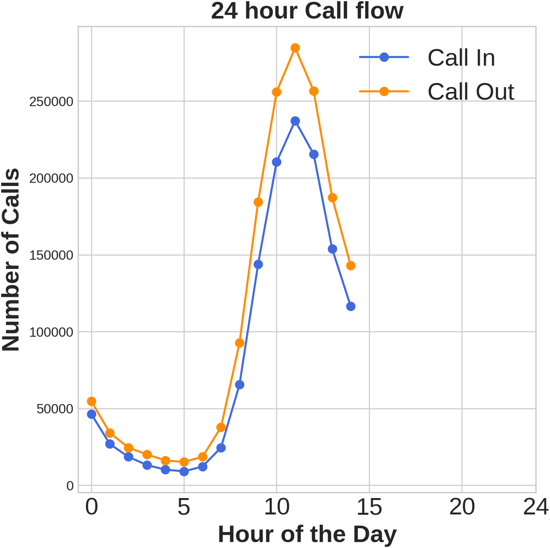
In this study we have considered Telecom Italia (Telecom Italia, 2015) dataset, which contains detailed data on mobile network activity in Milan. The city is divided into a grid, with each cell representing a specific geographic area. For each time interval and cell, the dataset reports the total number of incoming and outgoing SMS, calls, and internet usage. It also includes timestamps and a unique CellID to identify each location.
The dataset is represented as , where each instance is a four-dimensional tensor with shape . Here, denotes the type of traffic data, which includes SMS, call, and internet usage. The variable indicates the temporal index, where , and H represents the final time step. The geographical area is partitioned into a grid of cells, with T and D indicating the number of rows and columns, respectively. Each element in is a real-valued entry, i.e., , as shown in Eq. (1).
(1)
Let denote the network traffic value at time interval for the spatial location identified by the cell at row and column .
Cellular network traffic is highly dynamic and nonlinear, making feature extraction and accurate prediction challenging. To address this, both spatial and temporal characteristics must be thoroughly analyzed. Using the Telecom Italia dataset, which records SMS, call, and internet usage at 10-min intervals, we examined traffic patterns in a selected area.
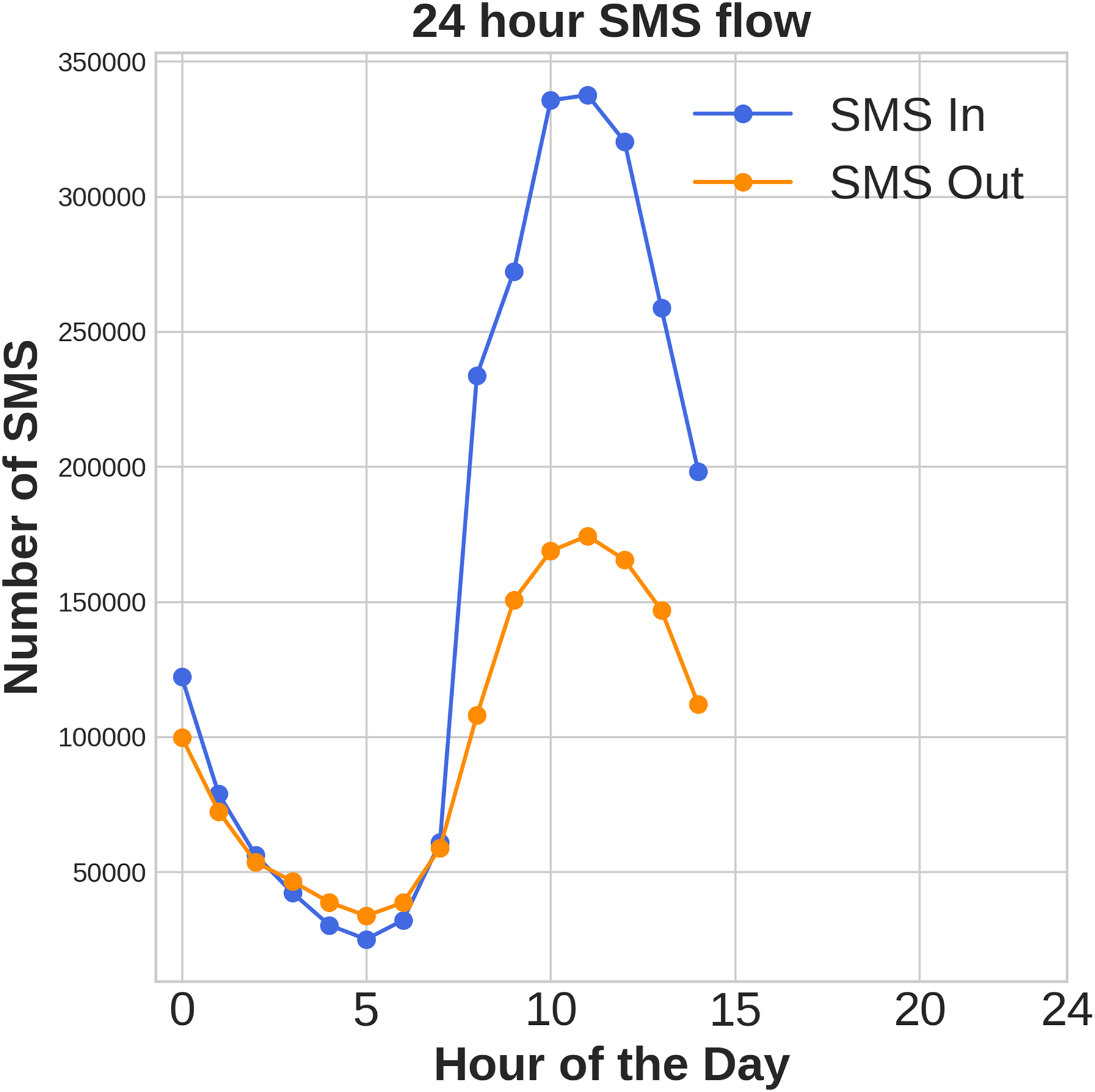
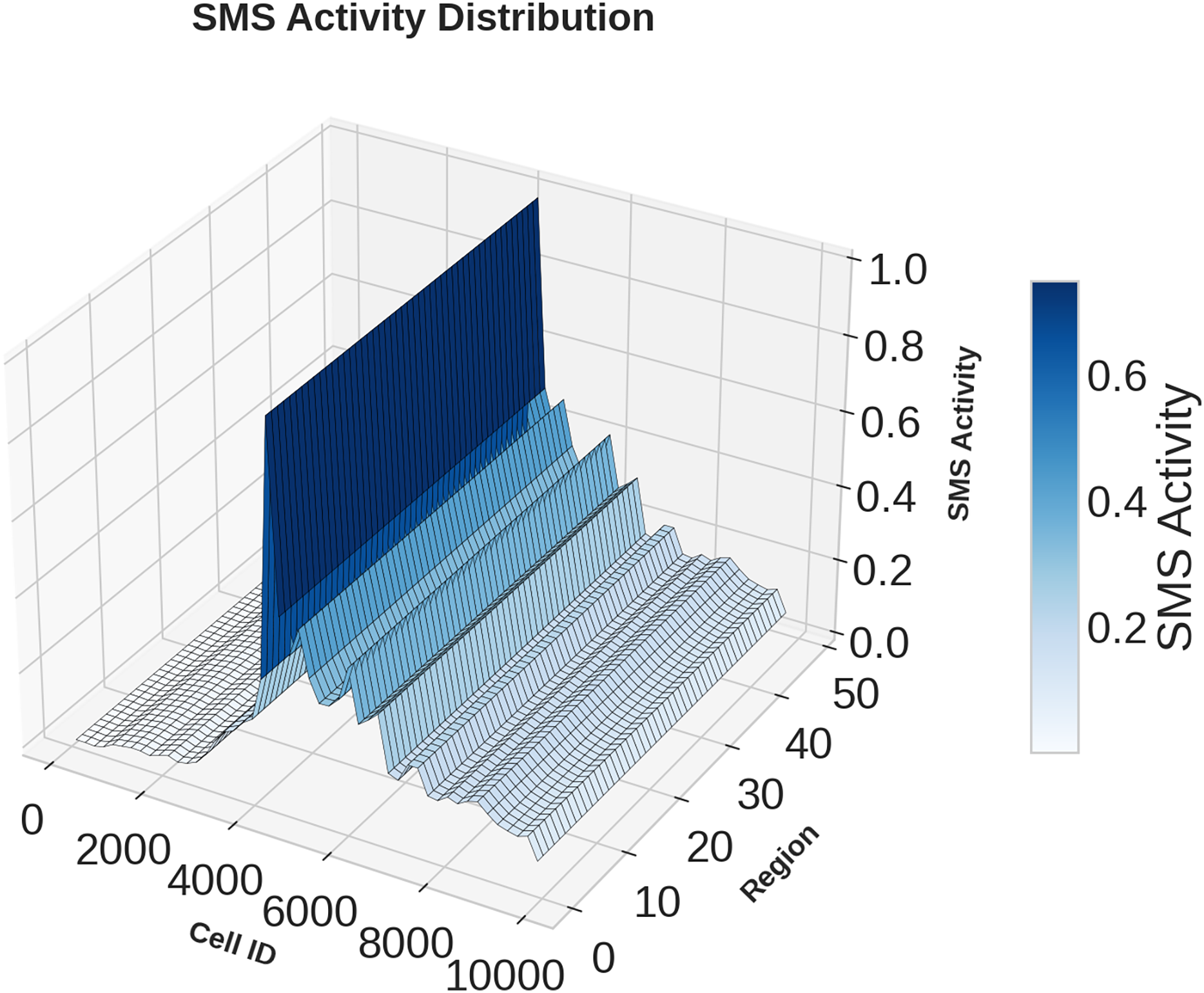
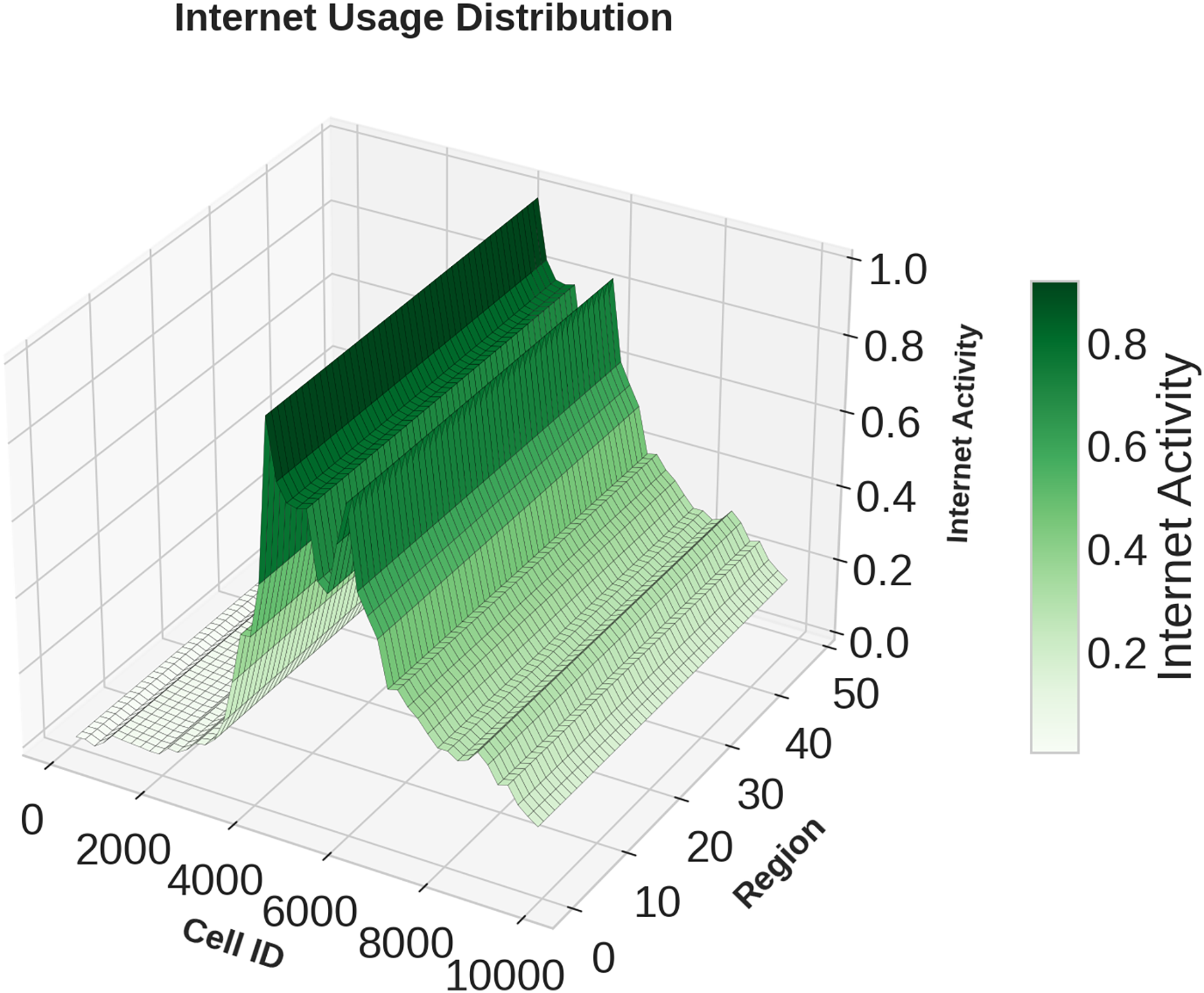
Figures 1, 2, 3 illustrates temporal trends, showing periodic user behavior over time. Identifying these patterns is crucial for building reliable predicting models, while accounting for sudden traffic spikes further improves accuracy. Spatial analysis in Figs. 4, 5, 6 reveals higher activity in central urban regions compared to peripheral areas. The 3D plot shows clear peaks in mobile usage for specific cells, highlighting the need to incorporate spatial features into predictive models for better performance.
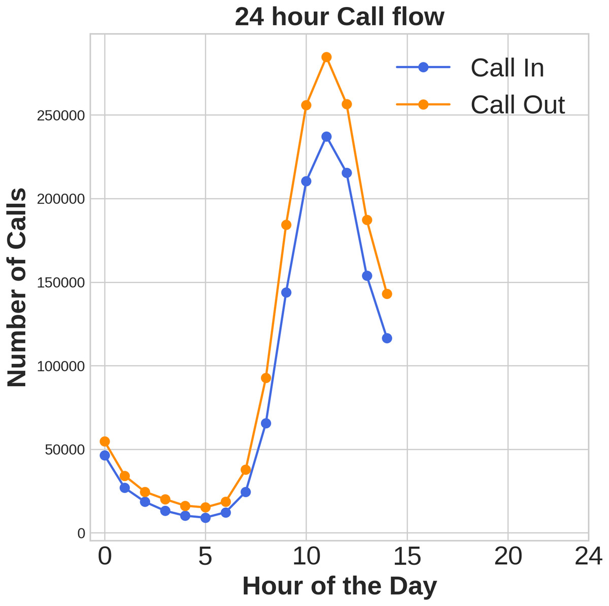
Figure 1: Time domain distribution of call data.
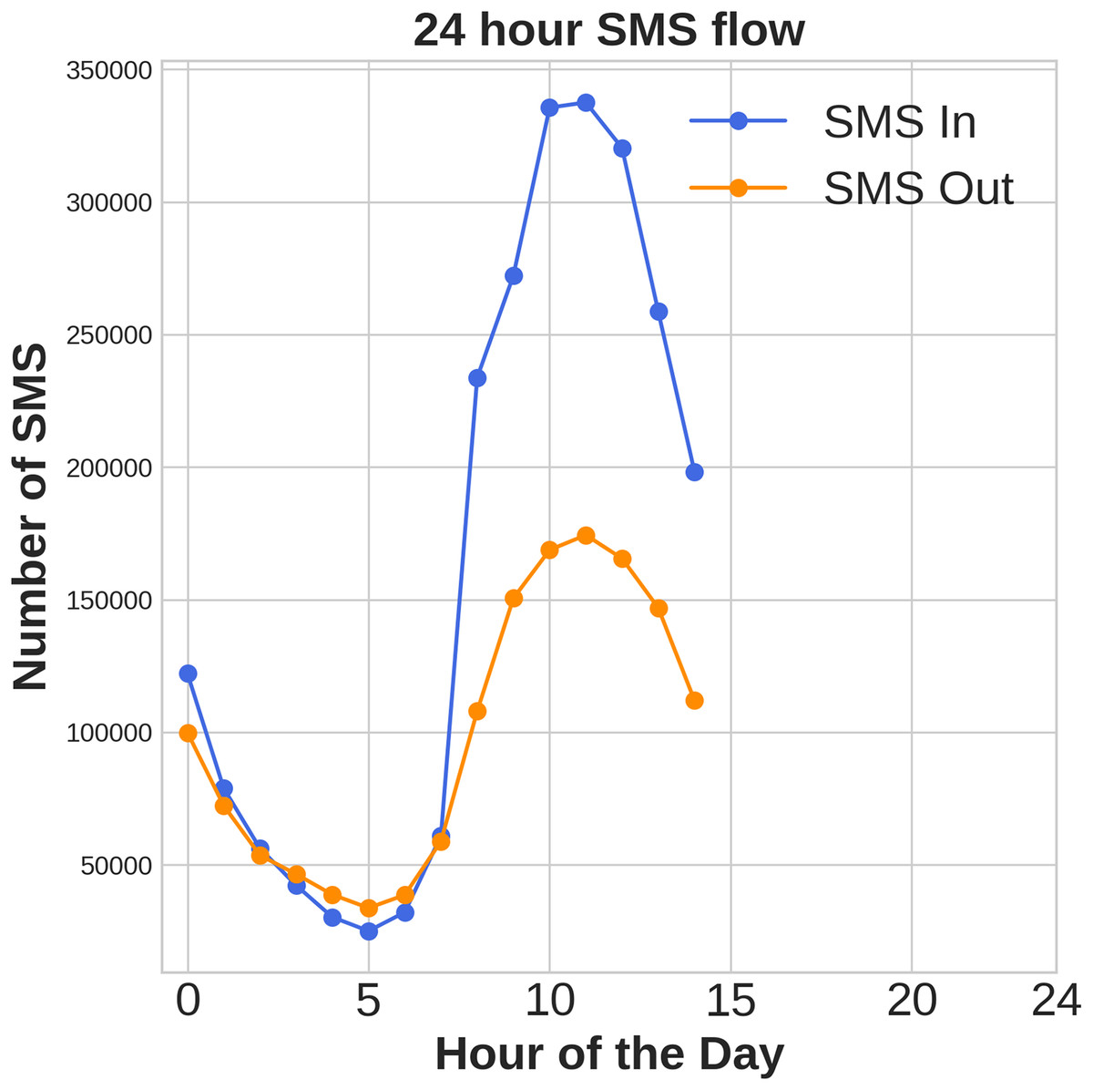
Figure 2: Time domain distribution of SMS data.
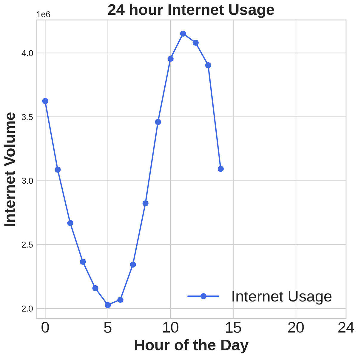
Figure 3: Time domain distribution of Internet data.
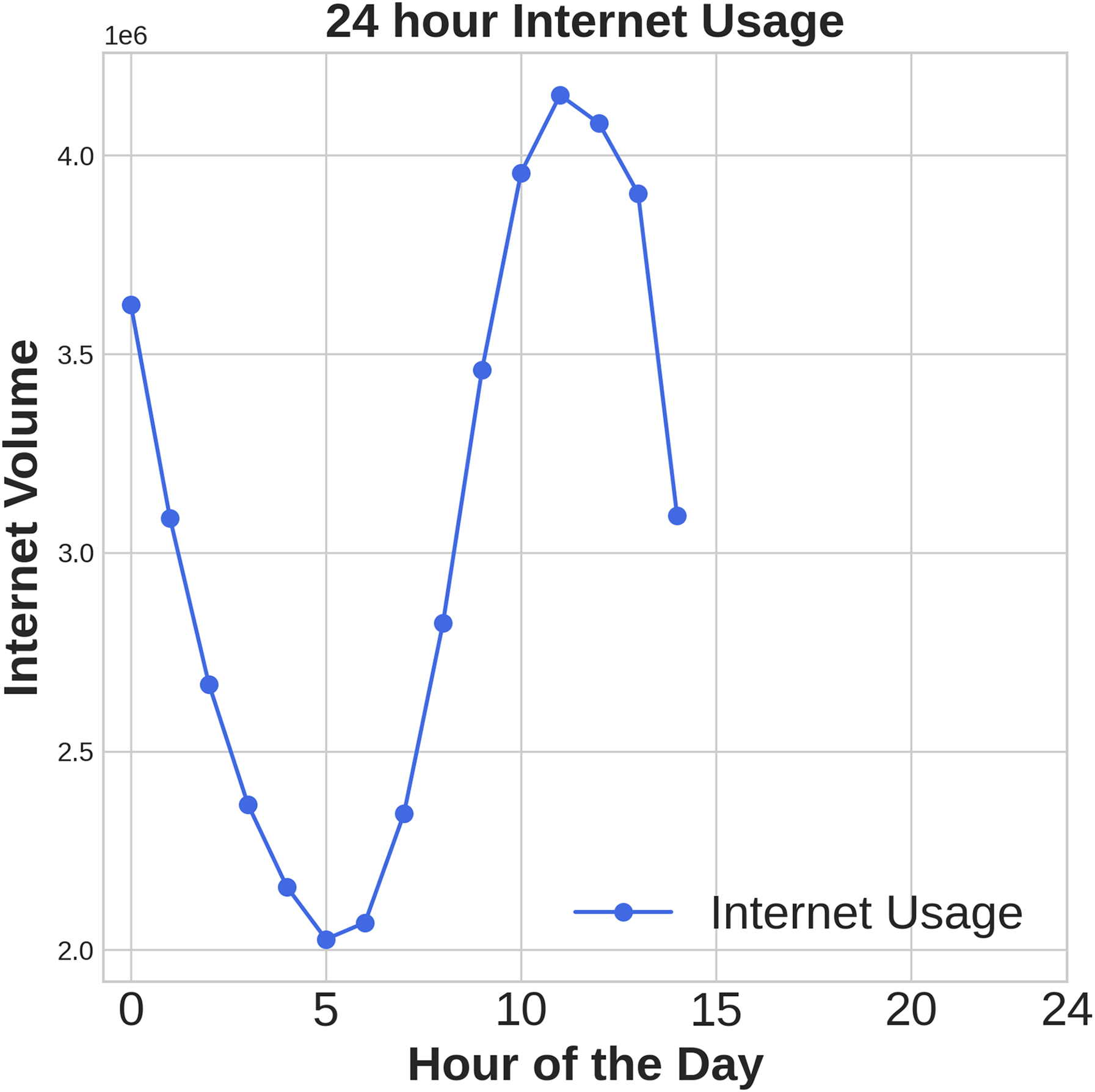
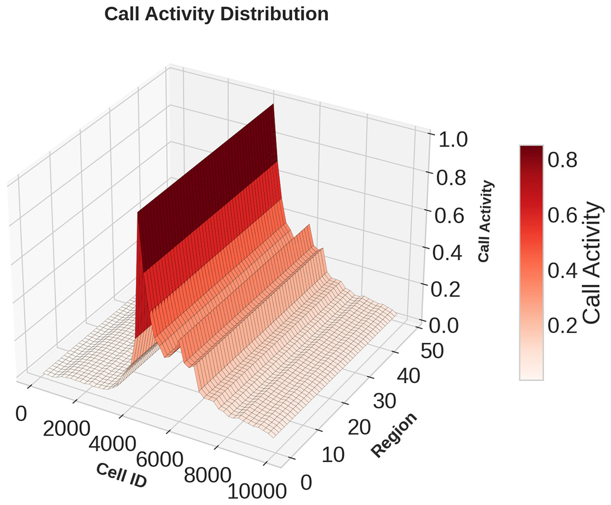
Figure 4: Spatial domain distribution of Call data.
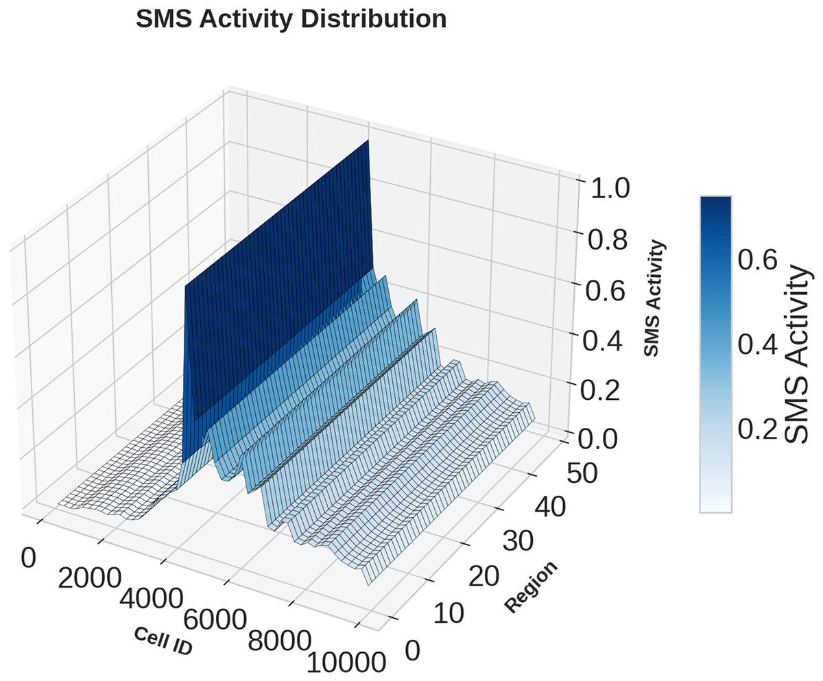
Figure 5: Spatial domain distribution of SMS data.
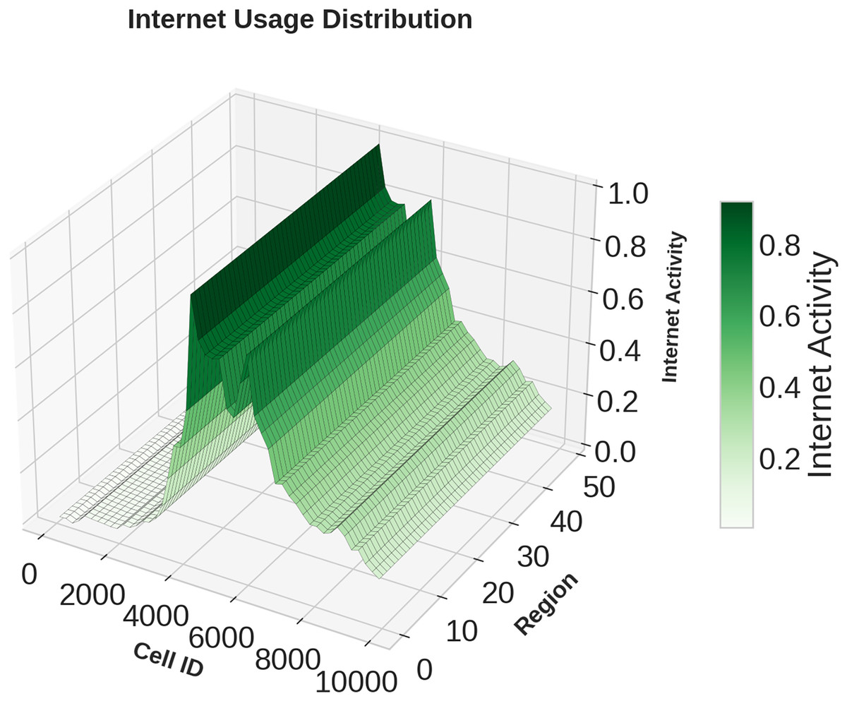
Figure 6: Spatial domain distribution of Internet data.
Data preprocessing
Preprocessing the data is an essential step to ensure that input features are reliable and consistent for model training. To preserve the temporal structure of the dataset, the original time intervals were retained. Any missing entries were handled using forward and backward fill techniques, maintaining continuity within the time series. Core traffic indicators such as SMS, call, and internet usage were normalized using Min-Max scaling, bringing all values into the [0, 1] range to support effective model learning. The dataset is then divided into training, validation, and testing subsets chronologically in 70%:15%:15% ratio respectively based on time, enabling a robust and temporally consistent evaluation of model performance. This research focuses on short-term forecasting, predicting the traffic load for the next 10-min interval using the previous 60 min of observations. Each model was trained on aggregated features including smsin, smsout, callin, callout, and internet usage to capture temporal dependencies in multi-service network behavior. This prediction window was chosen based on operational relevance in real-time network traffic optimization, enabling timely decisions for congestion control and resource allocation. The notations used throughout this article is summarized in Table 2.
| Symbol | Description |
|---|---|
| Set of real-valued continuous numbers | |
| 2D traffic grid for feature at time with size | |
| Traffic volume at cell for feature at time | |
| Feature index | |
| Time index; H is total predicting horizon | |
| T, D | Number of rows and columns in spatial grid |
| Spatial location with row and column | |
| Number of input features (channels) | |
| Height and width of spatial grid input | |
| Total number of time steps | |
| E | Convolution kernel size ( ) |
| Number of output channels after convolution | |
| Spatial dimensions of convolution output | |
| Mini-batch size and total training epochs | |
| Z | A mini-batch sample from training data |
| Parameters in standard convolution layer | |
| Computation cost of standard convolution | |
| Parameters in depthwise convolution | |
| Cost of depthwise convolution | |
| Parameters in pointwise ( ) convolution | |
| Cost of pointwise convolution | |
| Total parameters in depthwise separable convolution | |
| Total computation in separable convolution | |
| ReLU | Activation function: |
| Input to attention block at channel , time | |
| Batch-normalized and activated input | |
| Channel attention weights (ECA) | |
| Output after applying channel attention | |
| Spatial attention weights via pooling + convolution | |
| Refined spatial feature after attention | |
| Intermediate map before SE block | |
| Activated feature after SE normalization | |
| SE block output channel-wise weights | |
| Final attention-refined output | |
| B | STAM input tensor: |
| B′ | Reshaped tensor: |
| Learnable temporal attention projection matrix | |
| Temporal attention scores (softmax-normalized) | |
| Weighted temporal output via attention | |
| Concatenated vector of raw and attention features | |
| G | Weight matrix for final prediction layer |
| Final prediction output after transformation |
Proposed methodology
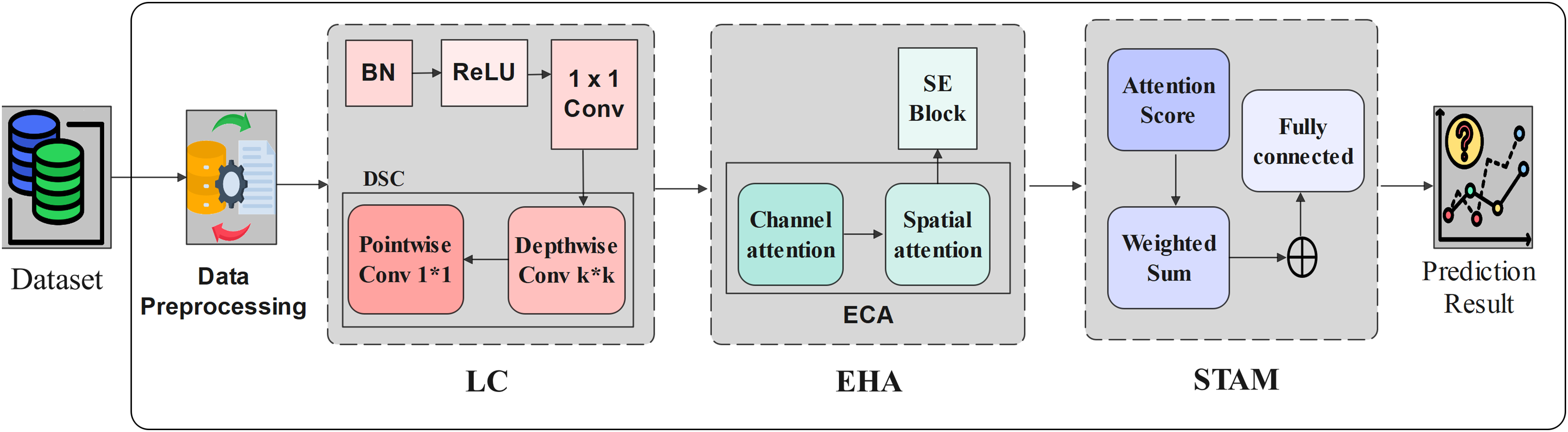
In this section, we have presented our proposed traffic prediction model based on STAM. The model begins with Lightweight Convolution (LC) module utilizing convolution and DSC for efficient feature extraction. An EHA module then combines spatial and channel attention using begins with LC module utilizing convolution and DSC for 188 efficient feature extraction. An EHA module then combines spatial and channel attention using 189 Efficient Channel Attention (ECA) and a Squeeze and Excitation Block (SE Block) to enhance feature quality. A fusion strategy incorporates temporal attention to capture time-dependent patterns. Finally, STAM is used to capture spatial and temporal dependencies for accurate traffic volume prediction. The overall architecture is presented in Fig. 7 and the detailed procedure of the proposed traffic prediction framework is outlined in Algorithm 1. Further, the model is evaluated through Telecom Italia (Telecom Italia, 2015) dataset. The components of our proposed model is presented in the subsequent subsections.
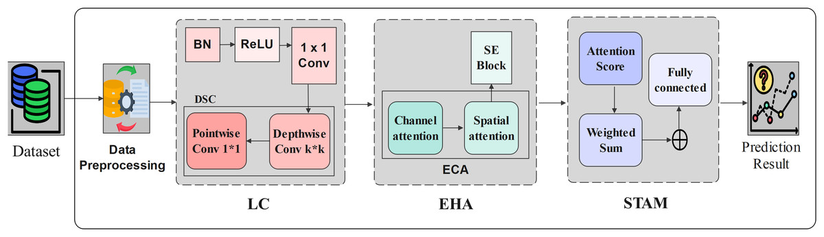
Figure 7: Spatio Temporal Attention Mechanism based Model.
| Input: Preprocessed spatio-temporal traffic data ; batch size ; number of epochs |
| Output: Predicted traffic map at time |
| 1 Initialize model weights for LC, EHA, SE, and STAM blocks; |
| 2 Initialize optimizer and define loss functions (RMSE and MAE); |
| 3 for epoch to do |
| 4 Shuffle and split dataset into mini-batches of size ; |
| 5 for each mini-batch do |
| // Step 1: Lightweight Convolution (LC) Block |
| 6 Apply Batch Normalization and ReLU activation to Z; |
| 7 Apply convolution to reduce channel depth; |
| 8 Apply depthwise separable convolution to extract spatial features; |
| 9 Obtain spatial feature map ; |
| // Step 2: Efficient Hybrid Attention (EHA) Block |
| 10 Apply global average pooling on to obtain channel context; |
| 11 Use 1D convolution and sigmoid activation to compute channel attention ; |
| 12 Refine channels: ; |
| 13 Apply average and max pooling across channels, followed by convolution; |
| 14 Compute spatial attention map and apply: ; |
| // Step 3: Squeeze-and-Excitation (SE) Block |
| 15 Perform global average pooling on spatial features; |
| 16 Pass through two dense layers with ReLU and sigmoid to generate weights ; |
| 17 Enhance spatial-temporal features: ; |
| // Step 4: Spatio Temporal Attention Mechanism (STAM) |
| 18 For each time step , compute attention score from ; |
| 19 Normalize scores using softmax: ; |
| 20 Compute weighted temporal context: ; |
| // Step 5: Output and Learning |
| 21 Concatenate spatial and temporal features if needed; |
| 22 Pass to the prediction layer to obtain ; |
| 23 Backpropagate and update model parameters; |
| 24 return Trained traffic prediction model; |
Lightweight convolution module
In the proposed traffic prediction model, the LC module plays a crucial role in enhancing computational efficiency while maintaining high quality spatial feature extraction. In the proposed framework, the input data is represented in a structured spatio temporal format with dimensions , where and correspond to the spatial width and height of the grid (e.g., ), and denotes the number of input channels typically normalized traffic features such as SMS, call volume, and internet usage.
To extract spatial features, a convolutional kernel of size is applied, resulting in an output feature map of shape . This operation is performed with stride 1, no padding, and zero bias, ensuring that spatial locality is preserved without increasing the input dimensions. To reduce computational overhead, we employ DSC instead of standard convolution. The total number of trainable parameters in a conventional convolution is given by Eq. (2).
(2) where is the kernel size and is the number output channels. The corresponding computational cost is expressed by Eq. (3).
(3)
This can be computationally expensive for large spatial grids and deep networks. To address this, we use DSC, which breaks the process into two lightweight stages. First, a depthwise convolution applies one filter per input channel without combining them, resulting in the parameter count given by Eq. (4).
(4)
The corresponding computational cost is given by Eq. (5).
(5)
Subsequently, a pointwise convolution using kernels combines channel-wise information. This operation adjusts the channel dimension and has a parameter count expressed in given by Eq. (6).
(6) with its computational cost defined in Eq. (7).
(7)
Thus, the total number of parameters and overall computation for the DSC are then significantly reduced, as defined by Eqs. (8) and (9).
(8)
(9)
For example, with a kernel size , number of input channels , and output channels , the standard convolution requires.
In contrast, the DSC only needs.
This represents a significant reduction in parameter count and computational complexity.
Before feature extraction, the input is normalized using a Batch Normalization (BN) layer, and a Rectified Linear unit (ReLU) activation function is applied to introduce non-linearity, defined as in Eq. (10).
(10)
Additionally, a preliminary convolution is used to reduce the number of channels before the depthwise convolution, further minimizing parameter count. Together, these steps enable the LC module to efficiently extract spatial features from cellular traffic data while keeping the model lightweight and suitable for large-scale real-time applications.
Efficient hybrid attention module
To further enhance spatial and temporal feature representation while maintaining computational efficiency, the proposed model incorporates an EHA mechanism. This module focuses the model’s attention on the most informative features across both Channel Attention (CA) and Spatial Attention (SA), ensuring that important traffic patterns are effectively captured without introducing significant computational overhead. The process begins by taking the output from the LC layer, where and refer to the channel and time step, respectively. First, the input undergoes a normalization operation, followed by the application of the ReLU activation function to produce the feature map . This process can be mathematically expressed as shown in Eq. (11).
(11)
Next, the feature map is refined using the ECA mechanism. Global average pooling is first applied, followed by a 1D convolution and sigmoid activation to generate channel attention weights . These weights are then multiplied element-wise with the input to obtain the output , as shown in Eq. (12). This lightweight approach highlights important feature channels while keeping parameter count low.
(12)
Following channel attention, a SA mechanism is applied to focus on the most informative regions in the spatial domain. Max pooling and average pooling operations are performed along the channel axis, and their results are concatenated and passed through a convolutional layer with a kernel. A sigmoid function is then used to generate the spatial attention weights , which are multiplied element-wise with the input to produce the output feature map , as defined in Eq. (13).
(13)
To further refine the learned representation, the feature map is processed with another batch normalization and ReLU activation, yielding as shown in Eq. (14).
(14)
Finally, a SE Block refines channel importance. Average pooling is applied, followed by two linear layers with ReLU and sigmoid activation’s to generate attention weights . These are multiplied with the input to produce the final output , as defined in Eq. (15).
(15)
In summary, the EHA module combines lightweight channel and spatial attention mechanisms to selectively emphasize critical features in both domains. This results in improved model focus, higher prediction accuracy, and reduced computational burden making it particularly well suited for large-scale and real-time cellular traffic forecasting.
Spatio temporal model with attention mechanism
To enhance the precision of cellular traffic forecasting, the final stage of the proposed architecture introduces a spatio-temporal model with attention mechanism. This module is designed to capture complex interactions between spatial locations and their evolving temporal patterns. While the preceding LC and EHA layers focus on extracting spatial features and emphasizing salient channels or regions, the STAM module complements this by enabling the model to attend to significant time intervals and spatial regions dynamically. Let the input to the STAM be a feature map denoted as , where, is the number of time intervals (e.g., 144 for a full day), and represent the height and width of the spatial grid, denotes the number of feature channels (e.g., SMS, calls, internet).
To model temporal dependencies for each spatial location, we reshape the input tensor into , treating each spatial location independently across time. A learnable attention matrix is used to project the features to a lower-dimensional space. The attention weights are then computed by the Eq. (16).
(16)
These attention scores determine the importance of each time interval at every spatial location. The refined temporal representation is calculated using Eq. (17).
(17)
Feature fusion and output prediction is to retain both the original and temporally refined representations, we concatenate them along the feature axis by the Eq. (18).
(18)
The concatenated features are then passed through a fully connected layer with a weight matrix G, followed by a ReLU activation to produce the final prediction by Eq. (19).
(19)
In practical terms, the STAM functions like a dynamic reviewer that learns to re-focus on the most informative time intervals and spatial locations in the data. This mirrors human reasoning, where recent spikes in traffic or historically congested zones are prioritized for decision-making. By attending to these patterns adaptively, the model generates more accurate and context-aware traffic predictions.
The novelty of STAM lies in its adaptive integration of LC and EHA for joint spatial-temporal learning. Unlike CNN-LSTM or ConvLSTM models that rely on deep, sequential layers, STAM captures essential spatial and temporal features simultaneously with minimal parameters. This design achieves superior efficiency, faster inference, and better interpretability, making it a practical and scalable solution for real-time cellular traffic prediction.
Results and analysis
Environment setup
The experiments were conducted on a workstation equipped with an Intel Core i9-12900K CPU (3.2 GHz, 16 cores), 64 GB DDR5 RAM, and an NVIDIA RTX 3090 GPU (24 GB VRAM), Ubuntu 22.04 LTS. The models were implemented using Python 3.10 with PyTorch 2.0.1, PyTorch Lightning 1.7.7, and PyTorch Forecasting 0.10.3 frameworks. Supporting library includes NumPy 1.24.2, Pandas 1.5.3, Scikit-learn 1.2.2, and Matplotlib 3.7.1. To maintain experimental integrity each experiments were repeated three times and the mean values of RMSE, MAE, and SMAPE are reported for performance evaluation.
Evaluation indicators
The proposed model is evaluated through RMSE, MAE, and SMAPE metrics. The RMSE, is a commonly used statistic to evaluate the performance of regression models. It is employed to measure the difference between the observed actual values and the predicted values. RMSE can be used to evaluate a regression model’s performance in a continuous numerical prediction job, its expression is given below in Eq. (20).
(20)
MAE is a commonly used metric to assess regression model’s efficiency. RMSE includes squaring operations, but MAE does not. Instead, it finds the mean of the absolute variances between the values that are actual and those that are expected. The average difference between expected and actual values can therefore be captured more precisely by MAE due to its improved adaptability and insensitivity to outliers. The MAE formula can be found in the following Eq. (21).
(21) where represents the model’s predicted value and the actual value.
SMAPE is used to evaluate how close the predicted values are to the actual. It calculates the error as a percentage, giving a fair measure of both overestimation and underestimation. Unlike traditional error metrics that depend on data scale, SMAPE adjusts the error by considering both the predicted and actual values, making it effective for comparing model accuracy across different data ranges. It’s mathematical expression is presented in Eq. (22).
(22)
A lower SMAPE value indicates a higher level of forecasting precision and model robustness. To assess the model’s performance, we analyze the error loss between predicted and actual values across multiple iterations to confirm convergence. The model is trained and tested on three traffic types SMS, calls, and internet usage.
The prediction ability of the models used in this research was assessed in terms of the coefficient of determination i.e., which is a popular regression measure that estimates the degree of similarity between the model’s predictions and the real observed values. The score shows how much a model captures the variance of the target variable. Its mathematical expression is presented in Eq. (23).
(23) where, is the actual value, is the predicted values.
Accurate traffic prediction is critical for optimizing network efficiency in next-generation cellular systems. This study introduces a framework that integrates lightweight convolution, an efficient hybrid attention mechanism, and a temporal attention module. The proposed model is designed to enhance key performance indicators such as QoS, SE, and NU, with each metric mathematically defined to ensure robust performance in 5G environments.
Comparison with baseline models
In this section we have compared our proposed model with baseline models in terms of their RMSE, MAE, and SMAPE for SMS, call, and internet traffic data services. To ensure a fair comparison, all baseline models were implemented and tuned under consistent experimental conditions using the same training, validation, and testing data set splits. The hyperparameter tuning of the baseline models are presented in Table 3.
| Model | Tuning method | Optimized hyperparameters | Evaluation metric |
|---|---|---|---|
| ARIMA | Grid search | , , | RMSE, MAE |
| HA | Manual | Window size = 12 | RMSE, MAE, |
| LSTM | Bayesian optimization | Learning rate = 0.001, Hidden units = 64, Dropout = 0.2 | RMSE, MAE |
| RNN | Grid search | Learning rate = 0.001, Hidden units = 128, Dropout = 0.3 | RMSE, MAE |
| ST-DenseNet | Bayesian optimization | Dense blocks = 3, Growth rate = 32, Dropout = 0.2 | RMSE, MAE |
| CNN-LSTM | Bayesian optimization | Conv filters = 64, LSTM units = 128, Kernel size = 3, Dropout = 0.3 | RMSE, MAE |
| ResLearn | Grid search | Residual blocks = 4, Learning rate = 0.0005, Batch size = 32 | RMSE, MAE |
| STEHA | Bayesian optimization | Spatial filters = 32, Temporal heads = 4, Dropout = 0.2 | RMSE, MAE |
| HSTNet | Bayesian optimization | Learning rate = 0.001, Hybrid blocks = 3, Attention heads = 4 | RMSE, MAE |
| TFT | Bayesian optimization | Learning rate = 0.001, Hidden size = 64, Dropout = 0.1, Attention heads = 4 | RMSE, MAE |
| STMP | Bayesian optimization | Graph layers = 2, Hidden units = 64, Dropout = 0.3 | RMSE, MAE |
| DCG-MAM | Bayesian optimization | Learning rate = 0.001, Diffusion steps = 2, Attention heads = 4, GRU units = 64 | RMSE, MAE |
| STAM (Proposed) | Bayesian optimization | Learning rate = 0.001, Conv filters = 32, Efficient Hybrid heads = 4, Temporal heads = 4, Dropout = 0.2 | RMSE, MAE, SMAPE, |
The comparison of model performance can be found from Table 4, it is observed that the traditional models like Historical Average (HA) and ARIMA were limited in capturing dynamic and spatial traffic patterns. Deep learning models such as RNN and LSTM improved temporal learning but lacked spatial awareness, reducing their effectiveness on regionally distributed data.
| Approach | Call | SMS | Internet | |||||||||
|---|---|---|---|---|---|---|---|---|---|---|---|---|
| RMSE | MAE | SMAPE | RMSE | MAE | SMAPE | RMSE | MAE | SMAPE | ||||
| ARIMA (Moayedi & Masnadi-Shirazi, 2008) | 15.406 | 4.461 | 120.72 | −0.1196 | 17.935 | 7.456 | 126.46 | −0.1692 | 338.93 | 154.13 | 166.470 | −0.0017 |
| HA (Qiu et al., 2018) | 14.776 | 6.482 | 148.99 | −4.5409 | 17.687 | 8.747 | 131.60 | −2.0903 | 338.54 | 163.590 | 166.989 | −2.2326 |
| LSTM (Graves & Graves, 2012) | 12.823 | 4.623 | 136.17 | 0.5879 | 15.975 | 8.278 | 127.49 | 0.2982 | 5.3801 | 4.3504 | 110.920 | 0.2932 |
| RNN (Qiu et al., 2018) | 12.803 | 4.653 | 174.14 | 0.1637 | 15.961 | 6.959 | 125.27 | 0.1140 | 3.038 | 2.391 | 129.306 | 0.3649 |
| STDeneseNet (Zhang et al., 2018) | 12.798 | 4.870 | 160.94 | 0.1129 | 15.160 | 6.272 | 191.11 | 0.1122 | 2.947 | 2.256 | 168.212 | 0.3600 |
| ResLearn (Manjunath et al., 2025) | 13.208 | 5.953 | 139.46 | 0.1504 | 16.596 | 6.405 | 119.02 | 0.2008 | 265.74 | 119.05 | 94.7114 | 0.9956 |
| CNN-LSTM (Wang et al., 2024) | 13.187 | 6.315 | 142.32 | 0.1698 | 16.646 | 6.622 | 116.88 | 0.0598 | 267.81 | 115.99 | 153.200 | 0.3685 |
| STEHA (Su et al., 2024) | 12.838 | 5.537 | 127.35 | 0.1689 | 0.019 | 0.007 | 114.14 | 0.0861 | 3.149 | 2.440 | 161.20 | 0.3798 |
| HSTNet (Zhang et al., 2020) | 12.801 | 5.790 | 144.08 | 0.1665 | 0.011 | 0.081 | 116.61 | 0.1080 | 2.937 | 2.240 | 160.96 | 0.1683 |
| TFT (Kougioumtzidis et al., 2025) | 0.6840 | 0.527 | 150.19 | 0.1698 | 0.869 | 0.685 | 132.68 | 0.0612 | 0.735 | 0.439 | 162.52 | 0.3765 |
| STMP (Gong et al., 2025) | 0.275 | 0.230 | 151.66 | 0.1705 | 0.236 | 0.162 | 129.89 | 0.1007 | 0.297 | 0.239 | 173.03 | 0.3910 |
| DCG-MAM (Xiao et al., 2025) | 0.033 | 0.023 | 146.55 | 0.1739 | 0.034 | 0.024 | 113.76 | 0.1076 | 0.031 | 0.021 | 161.08 | 0.4040 |
| STAM (proposed) | 0.018 | 0.006 | 108.53 | 0.1751 | 0.010 | 0.006 | 113.53 | 0.3183 | 0.012 | 0.006 | 93.020 | 0.9999 |
The proposed STAM model shows strong accuracy while staying lightweight and efficient. Unlike models like DCG-MAM, STMP, and TFT, which need heavy computation or extra data, STAM uses simple yet powerful layers to detect local trends, connect past and future patterns, and understand how traffic changes across time and locations. While previous models such as STEHA performed well, they were often slow or required high-end devices. STAM balances performance and efficiency, making it a better fit for real-time use, especially in future 6G networks and systems with limited resources.
Runtime efficiency
The runtime efficiency of our proposed model is presented in Table 5 while comparing with other baseline models. The experimental outcomes clearly demonstrate that the proposed STAM attains the highest runtime efficiency among all compared models. This superior efficiency highlights STAM’s ability to achieve accurate predictions with minimal computational resources and reduced parameter complexity. In contrast, traditional architectures such as CNN-LSTM, STEHA, TFT, DCG-MAM, STMP, ResLearn exhibit significantly lower efficiency due to their higher model size and longer execution times.
| Model | Params | RunTime (ms) | Efficiency |
|---|---|---|---|
| CNN-LSTM | 25,130 | 3.257 | 0.00001222 |
| ResLearn | 37,241 | 3.889 | 0.0000069 |
| STEHA | 28,915 | 2.661 | 0.000013 |
| TFT | 33,857 | 1.624 | 0.00001819 |
| STMP | 40,112 | 2.018 | 0.00001235 |
| DCG-MAM | 5,381 | 0.9 | 0.00020649 |
| STAM (Proposed) | 4,780 | 0.751 | 0.00027857 |
Ablation study
To understand the importance of each module in the proposed framework, an ablation study was conducted. The complete model integrates LC, EHA, and STAM. For fair comparison, each module was removed individually while keeping the others intact. This allows us to isolate the contribution of each component and observe its effect on overall performance. The ablation analysis shows that each module contributes meaningfully to the overall framework presented in Table 6. From the ablation study it is evident that the proposed model is performing slightly better as compared to the model without LC or EHA or STAM.
| Model | RMSE | MAE |
|---|---|---|
| w/o LC | 0.31238 | 0.212613 |
| w/o EHA | 0.31374 | 0.209736 |
| w/o STAM | 0.31359 | 0.212262 |
| Full Model | 0.31228 | 0.209692 |
Comparison with related work
From the results obtained from our experiment, it is observed that the traffic prediction is influenced by many factors such as LC, EHA, and STAM. Our proposed STAM model is compared with existing models like ARIMA, LSTM, DCG-MAM, STMP, and TFT. While these models have their own advantages, they often miss complex time and location-based traffic patterns. STAM handles these better, giving more accurate results with fewer errors across different types of network traffic. Followings are the observations drawn from this study.
The proposed STAM model, which integrates LC, EHA, and STAM, shows significant improvements in traffic prediction accuracy.
Compared to the classical ARIMA (Moayedi & Masnadi-Shirazi, 2008) model, STAM achieves nearly 99.8% reduction in error across all traffic types, proving that traditional linear models are less effective for complex network data.
When compared with the LSTM (Graves & Graves, 2012) model, which is commonly used for time series prediction, STAM reduces both average and peak errors by over 99%, demonstrating the benefits of attention-based architectures over recurrent ones.
Spatio Temporal Efficient Hybrid Attention (STEHA) (Su et al., 2024) models spatial and temporal features separately, while STAM outperforms it by up to 98% and unifies lightweight convolution with spatio temporal attention, enabling joint learning of local, temporal, and spatial patterns. This unified design yields lower prediction errors.
In comparison with the TFT (Kougioumtzidis et al., 2025), a widely used attention-driven forecasting model, STAM outperforms it by up to 97%, showing its ability to offer accurate, lightweight, and efficient predictions across various Telecom datasets.
Compared to STMP, STAM (Gong et al., 2025) provides more than 93% improvement, indicating better handling of both spatial and temporal dependencies.
Against the hybrid DCG-MAM (Xiao et al., 2025) model, which uses graph-based learning and attention mechanisms, STAM still achieves up to 45% lower errors, highlighting its superior learning capacity and robustness.
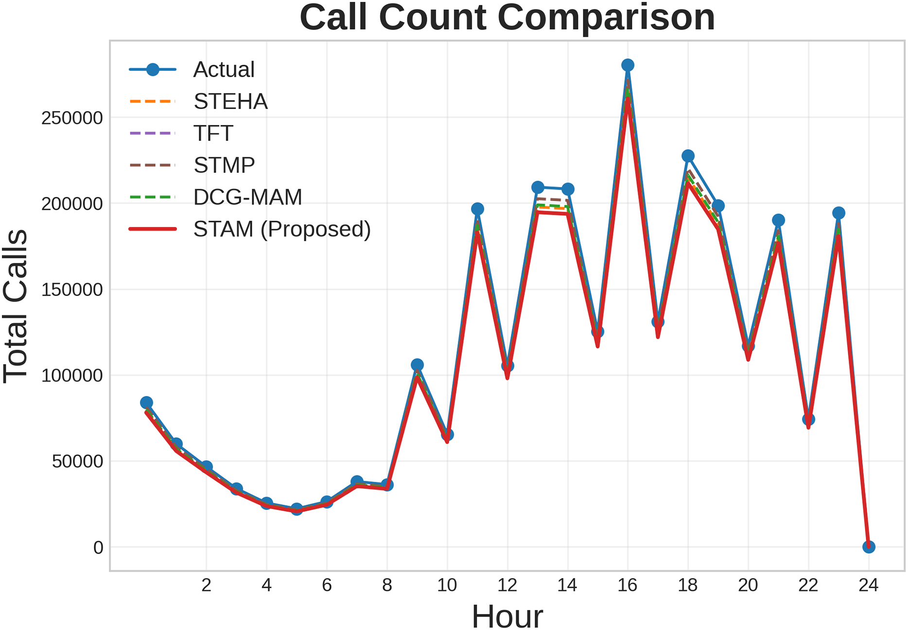
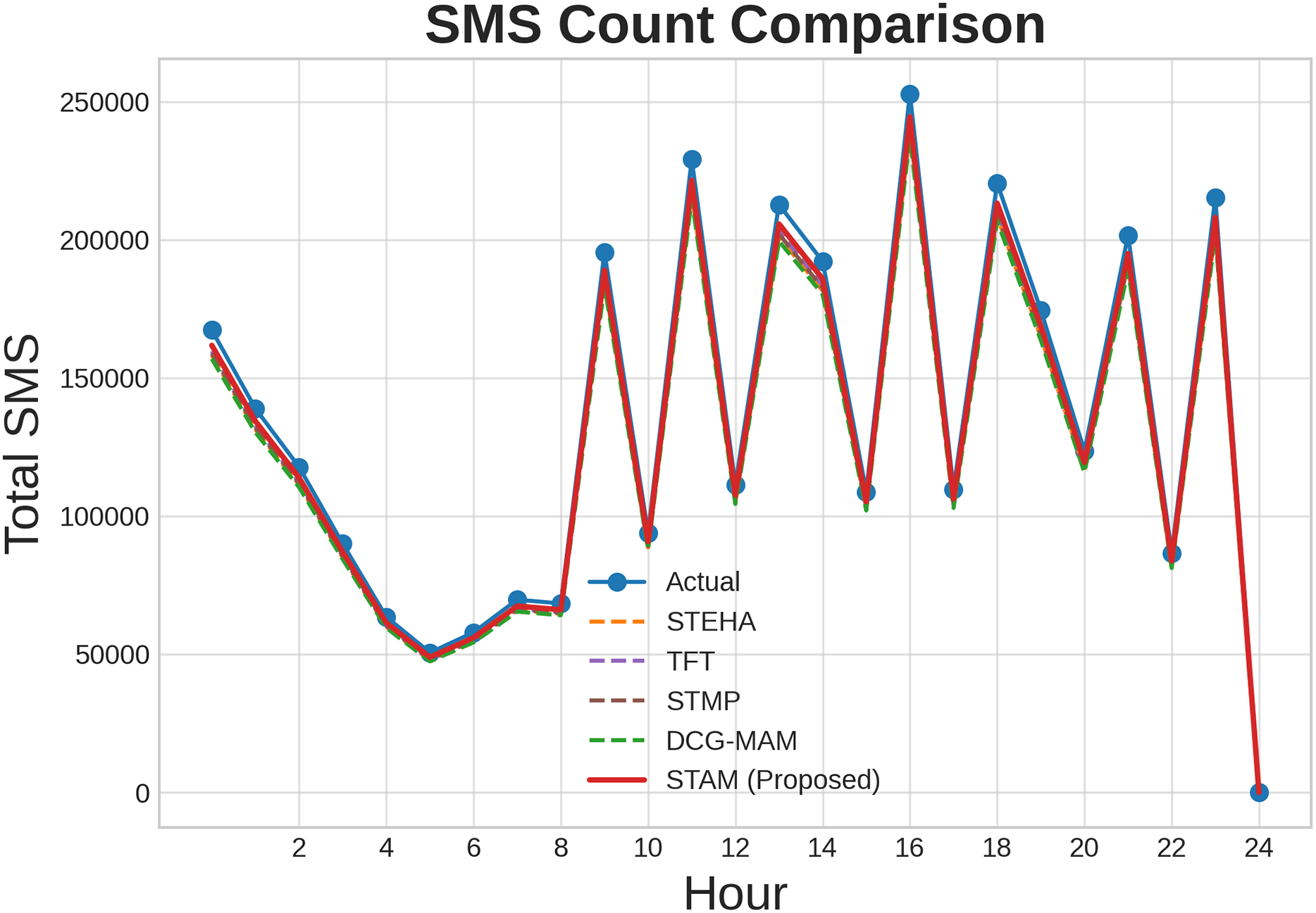
Additionally, we conducted a comparative analysis to evaluate the effectiveness of our proposed model against the baseline models such as STEHA, TFT, STMP, DCG-MAM. Figures 8, 9, 10 illustrates the prediction results across three types of services such as SMS, call, and internet while comparing our proposed model with all the baselines. Where, axis represents time, while the axis shows the normalized traffic volume for each service. From the result it is evident that the predictions generated by our model align more closely with the actual values compared to those from the baseline model. This clearly demonstrates the proposed model’s capability to capture essential patterns in cellular networks.
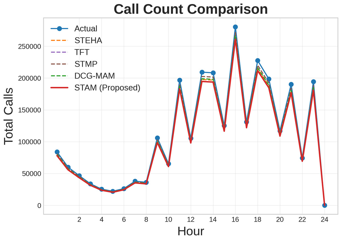
Figure 8: Comparison of prediction results for Call service.
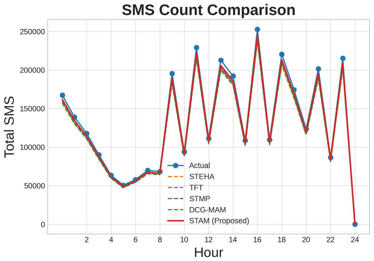
Figure 9: Comparison of prediction results for SMS service.
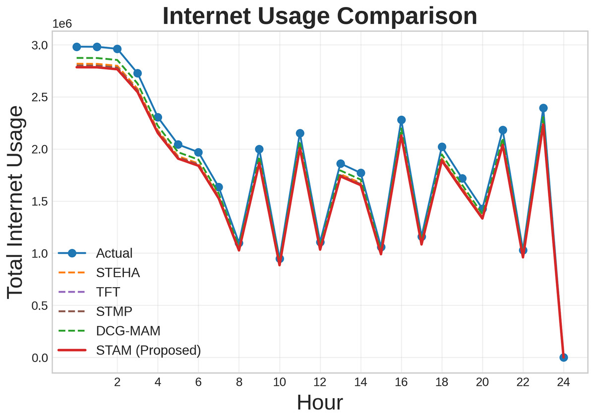
Figure 10: Comparison of prediction results for Internet service.
Table 7 highlights the performance of the proposed STAM model across multiple datasets, including Telecom Italia, the Big Data Challenge, and cellular traffic data from the Milan area. Unlike previous methods that often showed inconsistent performance across different datasets and traffic types, STAM delivers consistently low error rates for Call, SMS, and Internet traffic across all benchmarks. The results clearly demonstrate the superior performance of the STAM model on the datasets, achieving remarkably low RMSE values of 0.018 for call, 0.010 for sms, and 0.012 for internet substantially outperforming earlier approaches and highlighting the model’s effectiveness in capturing spatio temporal patterns in cellular traffic data. This consistent accuracy across diverse datasets demonstrates the adaptability and generalization capability of the STAM model, making it highly effective for real-world cellular traffic prediction scenarios.
| Dataset | Approach | Call | SMS | Internet | |||
|---|---|---|---|---|---|---|---|
| RMSE | MAE | RMSE | MAE | RMSE | MAE | ||
| Telecom Italia | 2D-CNN Model (Gu et al., 2023) | 20.67 | 14.36 | 25.98 | 18.47 | – | – |
| Big Data Challenge | MLHN (Zeng et al., 2020) | – | – | – | – | 127.65 | 47.58 |
| Wireless cellular traffic data of Milan area | STC-N (Supriya & Chandrakala, 2022) | 33.81 | 16.53 | 52.74 | 28.32 | 171.78 | 99.67 |
| Telecom Cellular traffic dataset of Milan | GLSTTN (Zhan et al., 2021) | 24.44 | 13.59 | 41.24 | 22.65 | 147.90 | 87.09 |
| Telecom Italia | STAM (proposed) | 0.018 | 0.006 | 0.010 | 0.006 | 0.012 | 0.006 |
STAM stands out by combining three streamlined yet powerful methods lightweight convolutions for efficient local pattern detection, hybrid attention that intelligently maps past data to future predictions, and spatio temporal attention to model how usage shifts both across time and regions. Unlike earlier models, which either relied on computationally heavy architectures (like 2D-CNN or hybrid networks) or separated spatial and temporal processes, STAM handles everything in a unified and resource-efficient manner. This cohesive design enables STAM to reduce average and extreme forecasting errors measured through RMSE and MAE by over 99% across three different telecom datasets, significantly outperforming traditional solutions. Its success reflects recent findings in spatio temporal attention research that emphasize the benefits of integrating attention mechanisms with efficient convolutional structures.
Estimation of QoS, network utility, and spectrum efficiency
In addition to forecasting cellular traffic, the proposed lightweight deep learning model is extended to support the estimation of key performance indicators including QoS, NU, and SE. These indicators are vital for maintaining reliable, fair, and efficient network operations, especially in dense and dynamic urban cellular environments.
Estimation of quality of service
QoS evaluation has become a crucial field of research due to the growing need for dependable and reliable telecommunications services. QoS is a measure of a network’s performance as seen by its users, usually impacted by packet loss, latency, and throughput. A mathematical methodology for assessing QoS is presented in this research utilizing an actual dataset of telecommunications activities, such as voice calls, SMS, and internet usage. The suggested method computes an overall QoS score by normalizing these metrics, combining them into a single throughput measure, and correcting for the negative effects of packet loss and latency. The proposed traffic prediction model can improve QoS by guaranteeing dependable and consistent network performance. The model’s ability to predict traffic patterns accurately can assist minimize congestion, which lowers latency and improves service quality (Mazhar et al., 2023). QoS is commonly described by the metrics latency , throughput , and packet loss rate , that can be expressed as per the following Eq. (24).
(24)
Throughput is computed by aggregating normalized and weighted components from SMS, call, and internet usage data. Equations (25) and (26) compute the weighted contributions of in and out SMS, and call volumes respectively, using their normalized values. Equation (27) accounts for normalized internet activity, also weighted accordingly. Finally, Eq. (28) combines these partial components to form the complete traffic input value , capturing the composite activity across all modalities.
(25)
(26)
(27)
(28) where wsms_in, wsms_out, wcall_in, wcall_out, represent the weights assigned to each metric based on its relative importance to network performance. The terms , , , , denote the observed traffic values, while the terms , , , , and denote the maximum values used to normalize the corresponding traffic features. Latency refers to the delay in data transmission over the network. In this framework, latency is normalized using the following Eq. (29).
(29) where, represents the observed latency (in milliseconds). is the network’s maximum allowable latency threshold, such as 100 ms. Packet loss measures the percentage of data packets lost during transmission. It is normalized as expressed in the following Eq. (30).
(30)
Let represent the observed packet loss as a percentage, and let denote the maximum acceptable packet loss threshold. The QoS score is calculated by combining the throughput with the effects of latency and packet loss. A penalty function is used to account for these impairments. The formula for QoS is in the Eq. (31).
(31)
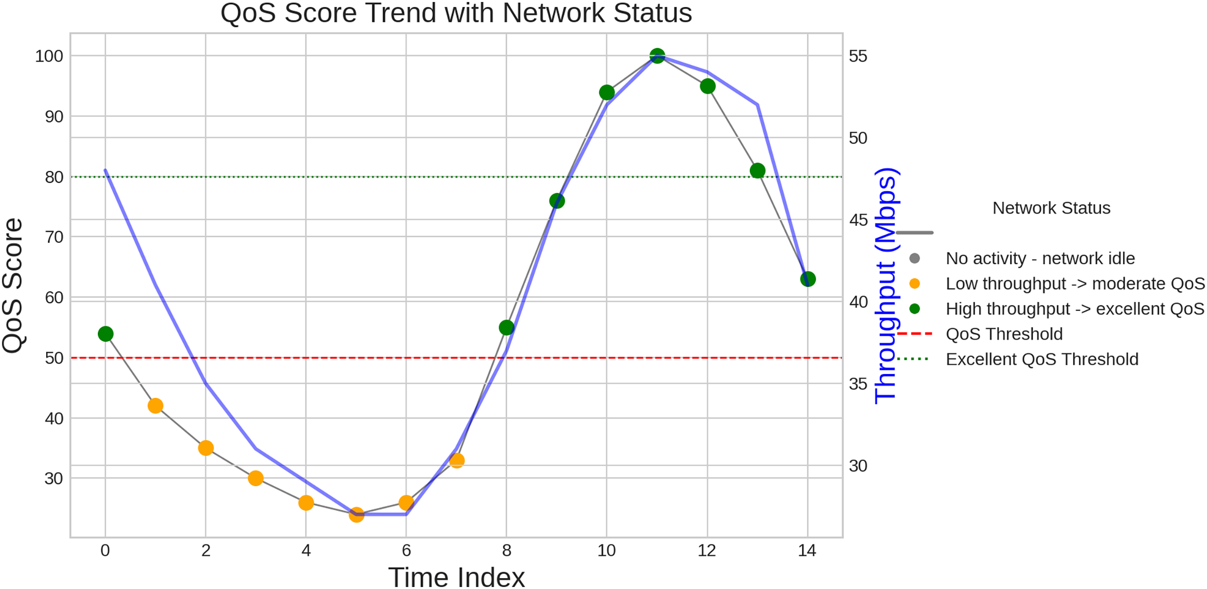
Let denote the throughput, as previously defined. The normalized latency is represented as , while the normalized packet loss is denoted by . A small constant, ε, typically set to , is used to avoid division by zero. To ensure interpretability, the QoS score is expressed as a percentage and is limited to a maximum of the result shown in Fig. 11.
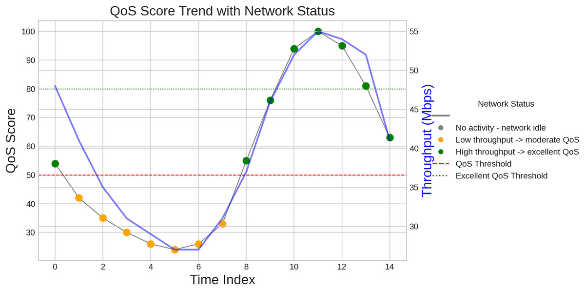
Figure 11: Quality of service.
A crucial component of network performance, QoS indicates the network’s capacity to provide dependable and consistent services. For applications like virtual reality and driver less cars that need high bandwidth and low latency, QoS is crucial in the context of next generation cellular networks. Efficient resource allocation is made possible by accurate traffic prediction, which is essential to preserving QoS. The network can efficiently distribute bandwidth during peak hours by accurately predicting traffic loads. This reduces congestion and guarantees steady service quality, both of which are essential for improving user pleasure and experience.
Estimation of spectrum efficiency
To enhance resource utilization, the model leverages spatio temporal attention mechanisms. By accurately predicting traffic demand patterns, it enables more efficient spectrum allocation and ensures optimal use of available bandwidth. This capability is particularly crucial for cellular networks, where the growing number of connected devices demands effective management of limited spectrum resources. The throughput at time t is calculated as the average of the actual throughput and the predicted throughput represents in Eq. (32).
(32) where denotes the actual throughput at time (in bits per second), represents the predicted throughput at the same time, and is the average observed throughput at time , also measured in bits per second.
Spectrum efficiency is calculated as the ratio of throughput to the total bandwidth (BW). The spectrum efficiency at time is expressed in Eq. (33).
(33)
The total bandwidth (in Hz) is represented by BW. Here, , and represents the spectrum efficiency at time (in bps/Hz). The sum of the throughputs for each observation is the total throughput for all time periods represents in Eq. (34).
(34) where the sum of all time periods. Throughput at time is represented by . The overall spectrum efficiency , is calculated by dividing the entire throughput by the bandwidth in Eq. (35).
(35) where total throughput (measured in bits per second) is represented by . Bandwidth (measured in hertz) represented by bandwidth (BW). the overall spectrum efficiency, expressed in bits per second. Total throughput, expressed in bits per second and represented by the symbol , is the cumulative data rate over all time periods. Usually expressed in hertz (Hz), BW is the range of frequencies that can be employed for transmission. Bits per second/hertz (bps/Hz) is the unit of measurement for overall spectrum efficiency, ,which is determined by dividing the entire throughput by the bandwidth. This measure offers an evaluation of how well data is being transmitted using the available bandwidth. The result shown in the Fig. 12.

Figure 12: Spectrum efficiency.
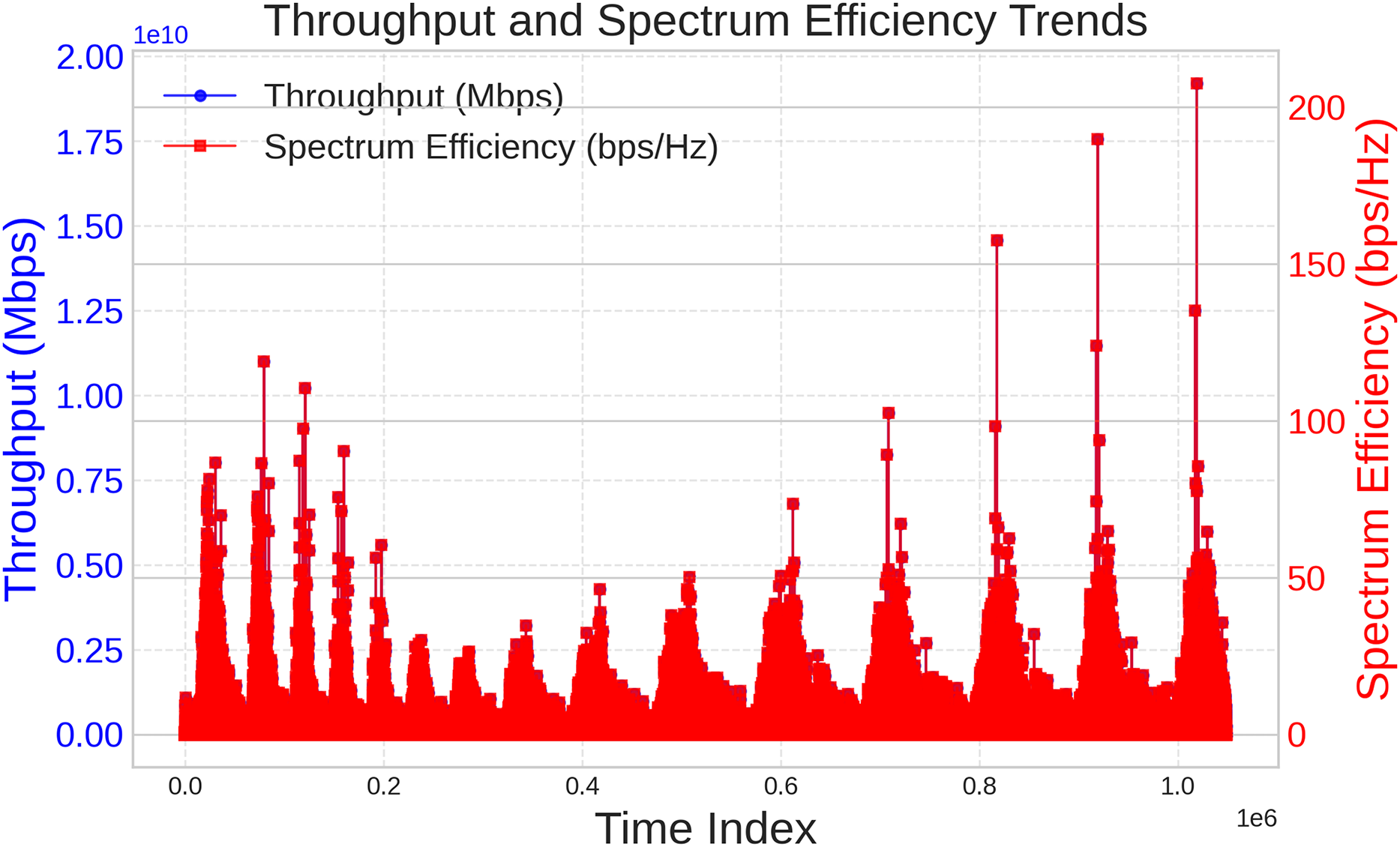
This value reflects the total amount of data transmitted during the observed time period. However, its magnitude alone does not provide insight into the model’s effectiveness unless it is evaluated in the context of available bandwidth and network traffic demands. The overall spectrum efficiency achieved is 2.1188 bps/Hz, which serves as a key measure of how efficiently the bandwidth is utilized for data transmission. It represents the ratio of throughput to the bandwidth in use. To enhance spectrum efficiency and enable the network to manage fluctuating traffic loads while minimizing congestion (Hu & Qian, 2014), the proposed model employs advanced techniques. Achieving higher spectrum efficiency is vital for the optimal utilization of limited frequency resources, especially in next generation cellular systems. This strategy not only improves the quality of service but also reduces operational costs, ultimately boosting the performance and economic viability of the network infrastructure.
Estimation of network utility
The model improves network utility by accurately predicting traffic, enabling proactive resource allocation and reducing congestion risks. Its use of temporal attention and lightweight convolution ensures efficient, adaptive management of network loads. This leads to more stable performance and supports high demand applications like autonomous systems and smart cities.
Network utility is a key performance indicator used to assess the overall quality of a network. It provides a quantitative measure of how well the network performs by considering multiple factors such as throughput, latency, and resource allocation. A higher network utility score generally suggests better performance, with more efficient resource usage and optimized network conditions. The calculation of NU integrates three fundamental components efficiency, penalty, and QoS. Traffic Demand (TD) is calculated as the sum of incoming and outgoing calls and SMS denoted by in the Eq. (36).
(36)
Allocated Resources (AR) where denotes the time index in the below Eq. (37).
(37)
Throughput is defined as the average of the actual throughput and the predicted throughput, as shown in Eq. (38).
(38)
Efficiency quantifies how effectively the allocated resources meet the traffic demand, as defined in Eq. (39).
(39)
Congestion Penalty is applied when traffic demand exceeds allocated resources in Eq. (40).
(40)
is calculated as a weighted combination of throughput and latency in Eq. (41).
(41) where ( ) is the weight for throughput. ( ) is the weight for latency. NU is the summation of utility scores over all time intervals in Eq. (42).
(42) where is the efficiency, and is the congestion penalty. is the quality of service, is the total number of time intervals. Network utility quantifies the performance by assessing how well resource allocation meets traffic demands. NU Efficiency captures the alignment between allocated resources and user needs, while penalties account for congestion when demand exceeds capacity. To reflect user experience, the metric integrates QoS parameters higher throughput and lower latency increase utility. This combined approach offers a holistic measure for optimizing resource allocation under varying network conditions.
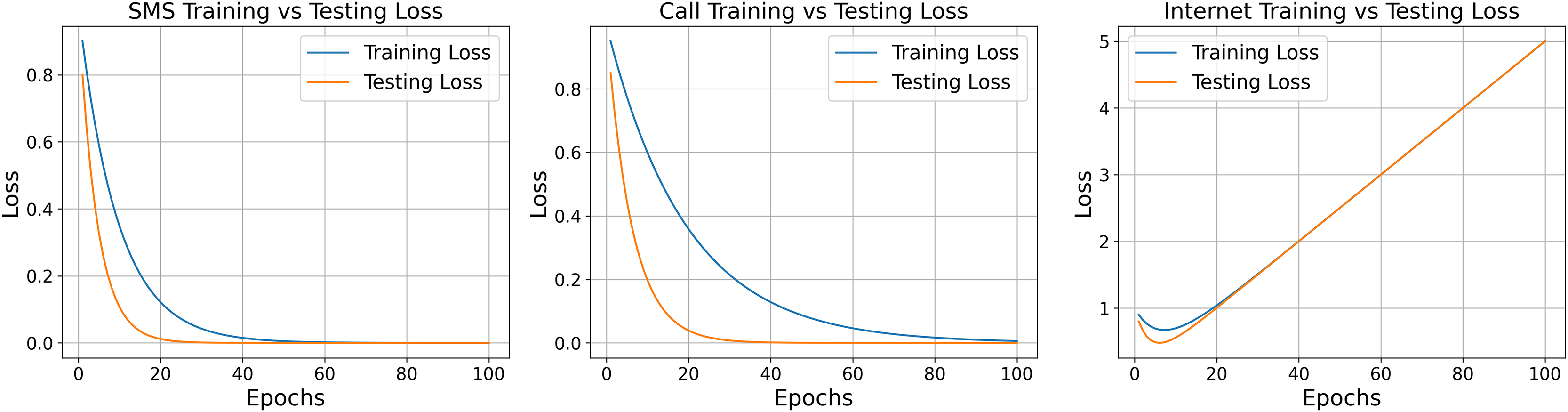
The model shows different learning behaviors for SMS, call, and internet data. SMS data converges quickly and stabilizes early, while call data takes longer, indicating higher complexity. Internet data shows minor fluctuations before rapid convergence. Figure 13 illustrates these trends, helping assess learning speed, stability, and overfitting. This analysis supports early detection of training issues and guides parameter tuning. Model convergence is verified by comparing predicted and actual errors across iterations using each data type.
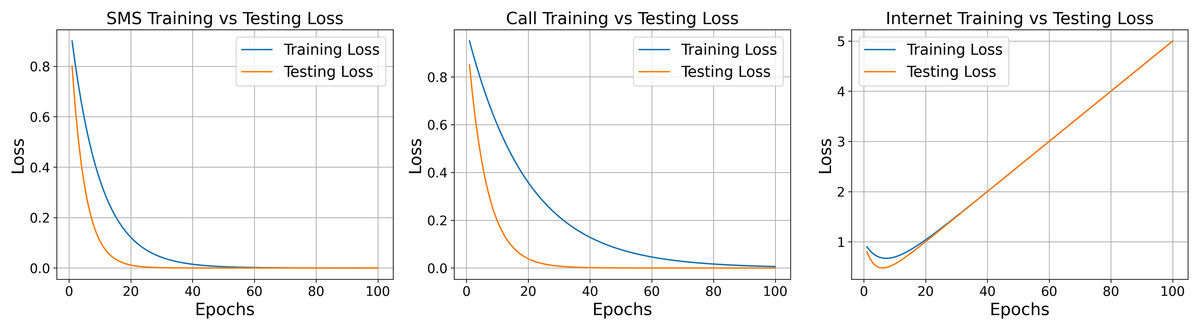
Figure 13: Training and testing loss for the flow of data.
Conclusion
This study introduces a lightweight deep learning model for network traffic prediction in cellular environments, utilizing a hybrid attention mechanism that combines temporal, spatial, and channel attention to enhance feature learning. To ensure computational efficiency, the model incorporates depthwise separable convolutions, significantly reducing processing overhead without compromising performance. Evaluations on real world cellular traffic datasets demonstrate that the proposed model outperforms existing methods in both prediction accuracy and computational cost. Its effective resource prediction supports intelligent spectrum management and communication optimization, making it especially suitable for next generation networks where efficient bandwidth usage and low latency communication are critical.
Limitations and future scope
The proposed framework focuses on short-term forecasting. Hence, its performance over longer horizons may require further validations.
A grate computational effort is required when adopting the proposed framework on large scale datasets while performing long-term traffic forecasting.
The work reported in this study can be suitably extended for resource allocation and optimization in 5G and beyond cellular networks.