
Individual different state-based multi-swarm particle swarm optimization
- Published
- Accepted
- Received
- Academic Editor
- Bilal Alatas
- Subject Areas
- Algorithms and Analysis of Algorithms, Artificial Intelligence, Autonomous Systems, Data Mining and Machine Learning, Optimization Theory and Computation
- Keywords
- Particle swarm optimization, Multi-swarm, Inertia weight, Quasi-Newton method
- Copyright
- © 2026 Xu et al.
- Licence
- This is an open access article distributed under the terms of the Creative Commons Attribution License, which permits using, remixing, and building upon the work non-commercially, as long as it is properly attributed. For attribution, the original author(s), title, publication source (PeerJ Computer Science) and either DOI or URL of the article must be cited.
- Cite this article
- 2026. Individual different state-based multi-swarm particle swarm optimization. PeerJ Computer Science 12:e3561 https://doi.org/10.7717/peerj-cs.3561
Abstract
Particle swarm optimization (PSO) is a renowned stochastic optimization algorithm that has attracted extensive attention from researchers worldwide. However, most PSO variants suffer from slow convergence and are susceptible to local optima. In this article, an individual different state-based multi-swarm PSO (IDSMPSO) is developed to address these problems. First, the swarm is dynamically divided into four sub-swarms based on fitness value of particles, and the number of particles in each sub-swarm varies randomly to enhance the swarm diversity. Second, different inertia weight strategies are applied to the corresponding sub-swarms, which can keep the balance between the exploration and exploitation. Subsequently, different dynamic learning mechanisms are used to each sub-swarm. To be specific, the best sub-swarm employs Levy flight and greedy strategy to boost particle’s search ability, the better sub-swarm utilizes cooperative learning scheme to strengthen information exchange between sub-swarms, the worse sub-swarm adopts a positive cosine learning factor to improve the convergence speed, and the worst sub-swarm leverages elite learning mechanism, random combination strategy and Gaussian mutation to enable particles escaping from local optima. Finally, the BFGS quasi-Newton method is utilized to refine the obtained optimal solution so as to further enhance the local convergence ability of the swarm. Extensive experiments on CEC2017 and CEC2022 benchmark test suites validate that the IDSMPSO proposed in this work surpasses several other peer algorithms in terms of global search ability, solution accuracy and convergence rate. Notably, the application of IDSMPSO to the three-dimensional uncrewed aerial vehicle (UAV) path planning has achieved highly satisfactory results, which further validate the effectiveness of our proposal.
Introduction
Optimization algorithms are mathematical methods for finding optimal solutions. They are widely applied in various scientific and engineering problems to solve the challenge of maximizing or minimizing objective functions under given constraints. These algorithm search for the optimal solution by exploring the solution space, which involves generating potential solutions, evaluating their quality and adjusting the search strategy based on the evaluation. Note that classical optimization algorithms include genetic algorithm (Holland, 1992), simulated annealing (Steinbrunn, Moerkotte & Kemper, 1997), particle swarm optimization (PSO) (Kennedy & Eberhart, 1995), ant colony optimization (Dorigo, Birattari & Stutzle, 2006), and so on. Due to the advantages of PSO—such as simplicity, ease of implementation, few parameters, and high efficiency in exploring global optimal solutions—it has successfully attracted the attention of many researchers.
Inspired by the flocking behavior of birds, PSO replaces the natural selection mechanism of evolutionary algorithms (Jong, 2017) with collective social behavior. It aims to find the optimal solution through the collaboration of particles within the swarm. The applicability of PSO is broad, making it suitable to solve various optimization problems, including continuous, discrete, single-objective, multi-objective, constrained, and unconstrained challenges. In view of this, it has been widely applied in model parameter identification (Yousri et al., 2019), neural network training (Sanchez, Melin & Castillo, 2020; Mohamad, Armaghani & Momeni, 2018), feature selection (Nguyen et al., 2016; Javidi, 2021), image processing (Suresh & Lal, 2017), path planning (Geng & Zhao, 2013), etc. In PSO, a group of “particles” traverses the solution space, each particle has a “personal best position” (pbest), representing the best solution so far. There is also a “global best position” (gbest), which is the best solution found among all particles (Kennedy, Eberhart & Shi, 2006). Particles continuously update their velocity and position to move towards the personal best and global best positions. The key to the algorithm lies in the update formulas for velocity and position, which balance exploration (searching new areas) and exploitation (fine-tuning search in known good areas) to improve search efficiency.
In many research fields, PSO is considered an effective optimizer. However, it is prone to becoming trapped in local optima, particularly in high-dimensional or complex optimization problems. The particle swarm relies on the gbest to guide its search direction. Consequently, if the gbest is not accurately identified, the entire swarm may converge prematurely to a local optimal region, making it difficult to escape from this limitation (Poli, Kennedy & Blackwell, 2007). Moreover, its sensitivity to parameters is also a challenging issue (Eberhart & Shi, 2004). Parameters such as inertia weight and learning factors play a critical role in optimization performance. However, these parameters are often determined empirically through trial and error. This may lead to inconsistent performance across different problems and potentially unstable or slow convergence in the search process. Furthermore, PSO’s search capability may fall short in some cases, especially when the problem scale increases or the search space becomes more complex, PSO may struggle to explore the solution space effectively (Kennedy, 2007).
To deal with the issue of premature convergence in complex environment mentioned above, multi-swarm techniques and dynamic learning strategies have gained considerable attention over the past decade, proving to be effective in maintaining swarm diversity and accelerating convergence. In Ye, Feng & Fan (2017), a multi-swarm particle swarm optimization with dynamic learning strategy (PSO-DLS) is proposed, in which a classification mechanism assigns ordinary particles for exploitation and communication particles with dynamic capabilities for exploration, thereby enhancing information exchange between sub-swarms. In Guelcue & Kodaz (2015), a novel PCLPSO is introduced that divides the population into one main swarm and multiple sub-swarms. The main swarm provides the global best solution to sub-swarms to improve the convergence speed, while sub-swarms share local best solutions to prevent premature convergence. Besides, Niu et al. (2007) propose a multi-swarm cooperative PSO (MCPSO) based on a master–slave model, where the master swarm updates particle’s velocity using cooperative or competitive learning—selecting the best individuals from slave swarms or its own best, whereas slave swarms apply general velocity update strategies. In the subsequent work (Zhao, Liu & Yang, 2014), MCpPSO is developed, in which the velocity update is based on the average of the sum of the best positions from all sub-swarms so as to promote the diversity of swarm. Note that although these methods have improved the performance of the canonical PSO to some extent, their optimization capability still needs to be enhanced in solving complex problems.
Inspired by multi-swarm information sharing and dynamic learning strategies, an individual different state-based multi-swarm PSO (IDSMPSO) is proposed here with the purpose of further enhancing the convergence rate and solution accuracy of PSO. The main contributions are as follows:
-
(1)
A multi-swarm technique is leveraged to divide the swarm into four sub-swarms of different states according to the particle’s fitness values and partitioning rules.
-
(2)
Different inertia weight strategies are applied to different sub-swarms to balance the global exploration and local exploitation.
-
(3)
Dynamic learning strategies, such as elite learning, cooperative learning and greedy strategy, are assigned to each sub-swarm to enhance search efficiency and prevent premature convergence.
-
(4)
The BFGS quasi-Newton method is used to refine the optimal solutions obtained so as to improve the local convergence capability of the swarm.
The remaining structure of this article is as follows: ‘Related Work’ introduces standard PSO and several PSO variants. In ‘Proposed IDSMPSO’, the IDSMPSO is detailed from four aspects of dynamic sub-swarm division, adaptive inertia weight, different learning strategies for different sub-swarms, and the BFGS quasi-Newton method. ‘Experiments and Analysis’ presents the simulation results and performance comparisons between IDSMPSO and several peer algorithms. In particular, IDSMPSO is applied to a three-dimensional uncrewed aerial vehicle (UAV) path planning problem so as to further demonstrate its effectiveness and robustness. Finally, ‘Conclusion and Future Work’ provides conclusions and future work.
Related work
Standard PSO
The standard PSO simulates cooperation and competition within a group, leveraging information sharing among individuals to search for the optimal solution. In each iteration, PSO first evaluates the objective function value at the current position of all particles, determines both the historical best position of each particle (i.e., the best solution found so far) and the best position of the entire group (i.e., the best solution found among all particles). Based on this information, the velocity and position of each particle are then updated. In this way, particles gradually approach the global optimal solution in the search space. PSO operates according to simple rules, and three factors are considered before updating velocity: its own inertial forward direction, the direction it considers best for itself and the globally best direction. PSO achieves a balance under these three choices. The formula can be described by Eqs. (1) and (2):
(1)
(2) where w is the inertia weight, c1 and c2 represent the cognitive and social learning factors respectively. r1 and r2 are random numbers between 0 and 1. pbi,j (t) and gbj (t) represent the particle’s personal best position and global best position respectively. xi,j (t) and vi,j (t) denote the velocity and position of the i-th particle in the j-th dimension at the t-th iteration.
PSO variants
PSO is known as a valid optimization algorithm. However, when solving complex problems, it often faces issues such as premature convergence, insufficient search precision, and difficulty in maintaining trade-off between global and local searches. To deal with these issues, researchers have developed many effective PSO variants, and they can be roughly divided into three categories: parameter adjustment, topological structure, and multi-swarm technique.
(1) Parameter tuning is a simple yet effective strategy to enhance the search ability of PSO. As for the inertia weight, it determines the extent to which a particle retains its movement velocity from the previous iteration. In Liu, Zhang & Tu (2020), a PSO with chaotic inertia weight (MPSO) is introduced to trade-off the global and local searches of particles. However, it suffers from the problem of premature convergence when applied to the optimization of high-dimensional complex functions. Note that in Zhan & Zhang (2008), APSO is formulated based on the evolutionary state to dynamically adjust the inertia weight. Zhang & Ding (2011) outline a MSCPSO, which adaptively adjusts the inertia weight based on particle fitness and uses adaptive strategies to regulate the influence of historical information. In addition, a new adaptive inertia weight is explored in Jiyue, Liu & Wan (2023) based on evolutionary differences among particles, with the goal of integrating adaptive inertia weights and multiple operators into the PSO. In Nagra, Han & Ling (2019), an improved self-adaptive PSO that incorporates gradient-based local search strategies is proposed, where the enhanced inertia weight significantly boosts the particle’s search performance. Alternatively, a PSO variant combining adaptive dynamic inertia weight and adaptive dynamic acceleration coefficients is introduced in Sekyere, Effah & Okyere (2024) in order to further enhance the particle’s exploration and exploitation capabilities.
Additionally, learning factors are another critical parameter in PSO. They are typically divided into the cognitive learning factor (c1) and the social learning factor (c2). The cognitive learning factor represents a particle’s ability to learn from its own historical best position, while the social learning factor represents its ability to learn from the swarm’s historical best position. Ratnaweera, Halgamuge & Watson (2004) discuss an approach where c1 decreases over time while c2 increases to balance global and local search capabilities. In Chen et al. (2018b), a hybrid particle swarm optimizer with sine cosine acceleration coefficients (H-PSO-SCAC) is proposed, which effectively controls local search and global convergence by introducing sine and cosine acceleration methods. In Tian, Zhao & Shi (2019), a chaotic particle swarm optimization based on an s-shaped acceleration coefficient (CPSOS) is proposed, where the sigmoid acceleration coefficient is designed to balance early-stage exploration with late-stage exploitation. An improved particle swarm optimization (A-PSO) is proposed in Chen et al. (2018a), where nonlinear dynamic acceleration coefficients are introduced to enhance solution quality and accelerate global convergence. However, most of these PSO methods only focus on adjusting inertia weights or acceleration coefficients independently, lacking a unified multi-strategy framework. As a result, the performance of PSOs can be undoubtedly impaired.
(2) Topology adjustment is widely applied in various PSO variants. Since the topology determines how each particle exchanges information with others, it directly affects the convergence rate and global search capability of the PSO. In Mendes, Kennedy & Neves (2004), the static topology is classified into fully connected, ring, four-cluster, pyramid and square structures. In the fully connected topology, each particle communicates with every other particle in the swarm, which leads to fast convergence but with the risk of getting trapped in local optima. In the ring topology, each particle only exchanges information with a few neighboring particles, which helps maintain diversity and prevents premature convergence. In Sun & Li (2014), a two-swarm cooperative PSO uses a ring topology for neighbor-based learning, while a four-cluster topology divides the swarm into subgroups to balance local and global information exchange, maintaining diversity and avoiding local optima. In literature Blackwell & Kennedy (2018), it is shown that fully connected topologies exhibit outstanding advantages in unimodal functions while ring topologies are better for multimodal functions.
Dynamic topologies change during the optimization process and can enhance the search capability of the PSO variant by adjusting the connections between particles. In Wang, Yang & Orchard (2016), a dynamic tournament topology strategy is introduced to strengthen PSO, where a few good positions are randomly selected from the entire swarm to guide each particle. In order to balance exploration in the early stages and exploitation in the later stages, a multi-swarm PSO based on dynamic topology and purposeful detection is proposed in Xia, Gui & Zhan (2018). In Zhang et al. (2022), KGPSO is presented based on a self-organizing topology and adaptive parameters. During the evolutionary process, the K-means clustering method is periodically used to divide the swarm into multiple distance-based sub-swarms to enhance the global search ability. Besides, Ni & Deng (2013) employ a random topology structure and explore the relationship between swarm topology and PSO’s performance. In Lim et al. (2018), an adaptive topology connection is utilized, where the connections are adaptively modified during different search stages to facilitate particle’s exploration. In summary, although the static topological structure is relatively easy to implement, it may trap the PSO into local optima due to their fixed connections. In contrast, despite the dynamic topologies can boost the search performance via adjustable connections, it will increase the computational complexity of the algorithm.
(3) Multi-swarm techniques have gained significant attention from researchers in recent years. The core idea is to divide the entire particle swarm into multiple sub-swarms, each of which conducts independent searches and shares information through predefined communication mechanisms.
To increase swarm diversity, a dynamic multi-swarm PSO (DMS-PSO) is proposed (Liang & Suganthan, 2005), which divides the population into small sub-swarms with periodic regrouping (R) to enhance diversity, though at the cost of slower convergence. To improve local search in specific regions, the PSO described in Zhao et al. (2008) integrates the quasi-Newton operator into DMS-PSO to enhance local search and accelerate convergence. Besides, in literature Nasir et al. (2012), a dynamic neighborhood learning PSO (DNLPSO) is structured based on the learning mechanism from CLPSO. Another approach, known as the multi-adaptive strategy PSO (MAPSO), is discussed in Wei et al. (2020). This method divides the population into multiple sub-swarms that can be recombined during evolution process, with particles in each generation adaptively selecting learning exemplars based on their performance. In Jiyue, Liu & Wan (2023), the population is dynamically divided into four sub-swarms according to their fitness values, with each sub-swarm adopting a different velocity update mechanism to improve algorithm performance. Similarly, in Gou et al. (2017), the population is divided into three sub-swarms based on emotional states: happy, normal, and unhappy. Particles within each sub-swarm use different velocity update mechanisms to obtain the global optimum. In Yang, Li & Huang (2023), a PSO variant based on a dynamic multi-swarm framework is proposed, combined with a stagnation detection mechanism (SDM) and a spatial exclusion strategy (SES). Alternatively, the ESD-PSO is developed in Yang & Li (2023a) to improve the information exchange efficiency among sub-swarms through an adaptive cooperative mechanism. To balance exploration and exploitation, the fuzzy C-means (FPC)-based partitioning method is used to divide the initial population into multiple sub-swarms in Tao et al. (2022). Although these studies have enhanced the diversity of swarm and local search ability via dynamic multi-swarm structures, they often suffer from slower convergence rate and increased complexity.
Proposed idsmpso
Motivated by the PSOs mentioned in the previous section, to deal with the inherent demerits of particle swarm optimization, such as loss of diversity and stagnation in local optima, IDSMPSO is proposed in this work, which will be elaborated from four aspects of dynamic sub-swarm division, adaptive inertia weight, different learning strategies for different sub-swarms, and the BFGS quasi-Newton method, respectively.
Dynamic sub-swarm division
It is well known that particle swarm division and the size of each sub-swarm play an important role in maintaining swarm diversity. In Ye, Feng & Fan (2017), the division of sub-swarms is based on the total number of particles. For instance, if the number of particles is M * N, the population is divided into M sub-swarms, each containing N particles. While this approach accelerates convergence rate, it can be difficult to maintain diversity under certain conditions. In literature Yang et al. (2018), a fixed number of particles are also employed for sub-swarm division, which may hinder the swarm diversity. Besides, in Kong, Jiang & Huang (2019), a parameter-based method for population division is introduced, where ps represents the swarm size and m is the division parameter. The swarm is divided by taking the quotient of ps divided by m, and any remainder is discarded. As iterations progress, the size of sub-swarms declines. In Yang, Li & Yu (2022), sub-swarms are divided into three categories and they are responsible for different search tasks. However, most researchers divide sub-swarms based on the number of particles or custom parameters, allocating a fixed number of particles to each sub-swarm rather than adaptively adjusting based on the dynamic evolution of all particles. In view of this, the swarm is dynamically divided into four sub-swarms based on particle’s fitness values. The formula is defined by Eq. (3):
(3)
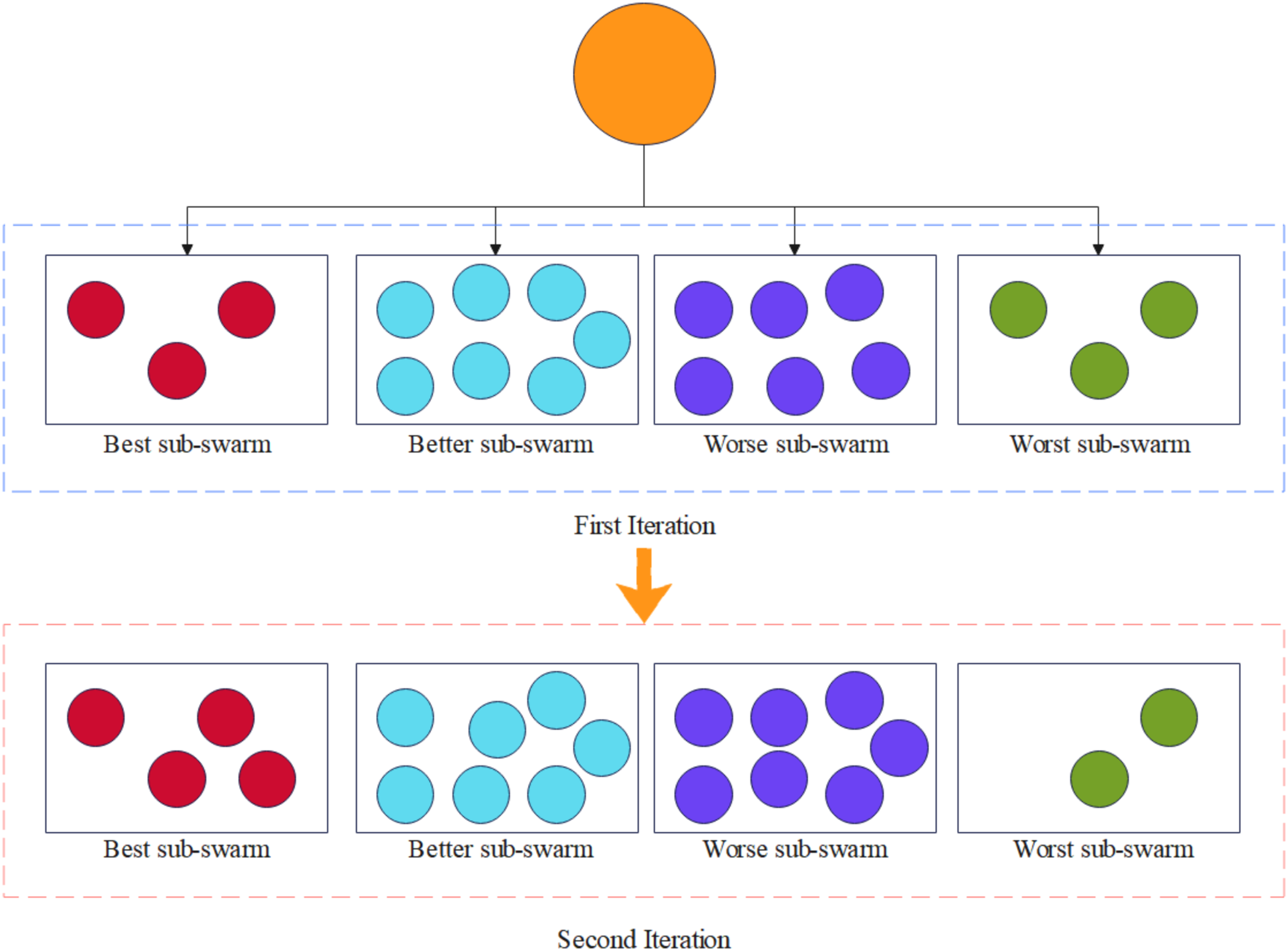
where, fmin represents the minimum fitness value of all particles in the swarm, which is also the optimal fitness value. fmax is the maximum fitness value of all particles in the population, which is also the worst fitness value. denotes the position of the i-th particle during the t-th iteration, where the subscript i refers to the particle within the population. The values for m1, m2, and m3 are set to 2, 3, and 4, respectively. represents the k-th sub-swarm in the t-th iteration. Since the range of k is (1,4), the swarm is divided into four sub-swarms, denoted as , , and . When a particle’s fitness value falls between f1 and f2, the particle belongs to S1 (the best sub-swarm). If the fitness value is between f2 and f3, the particle is assigned to S2 (the better sub-swarm). Similarly, if the fitness value is between f3 and f4, the particle belongs to S3 (the worse sub-swarm), and if the fitness value is between f4 and f5, the particle is categorized into S4 (the worst sub-swarm).
Assuming there are 20 particles in the population, the division of particles after two iterations is shown in the diagram. The orange circle represents the entire population, and we divide the swarm into four sub-swarms based on the division method. As shown in Fig. 1, the number of particles in each sub-swarm varies randomly as the number of iterations increases, which can effectively enhance swarm diversity and accelerate the convergence rate of IDSMPSO.
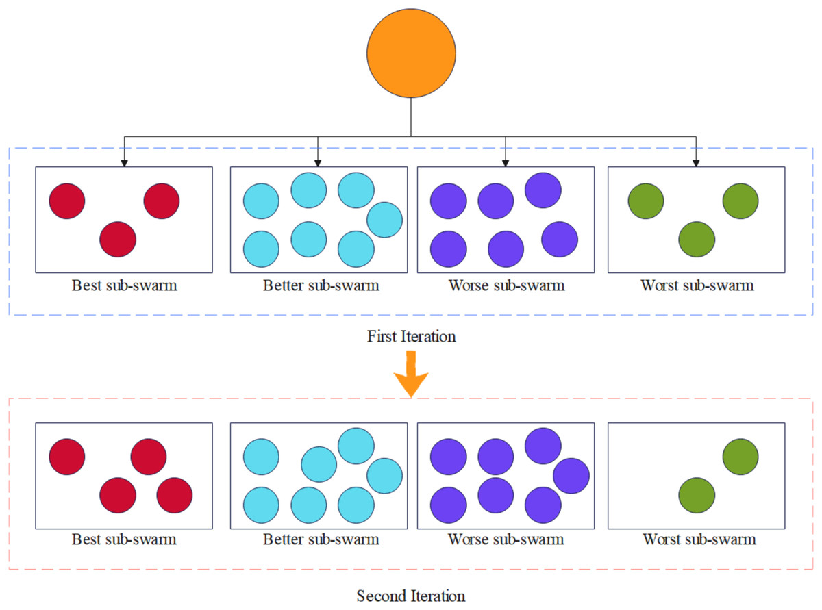
Figure 1: The varying process of each sub-swarm.
Adaptive inertia weight
Inertia weight plays a crucial role in the PSO, as it significantly influences particle’s search behavior and the convergence of the swarm. The introduction of inertia weight is intended to balance the particle’s global exploration capability with its local exploitation ability. Specifically, inertia weight controls the extent to which the current velocity affects the velocity in the next iteration. A larger inertia weight encourages particles to maintain higher velocities, enhancing global exploration. Conversely, a smaller inertia weight reduces the velocity, making particles rely more on local neighborhood searches, thus improving local exploitation. However, if the inertia weight is too large, particles may miss the optimal solution, while an excessively small inertia weight could cause particles to prematurely fall into local optima. Therefore, selecting an appropriate inertia weight strategy is key to maintaining a trade-off between global and local searches, as well as ensuring convergence in various complex optimization problems. In Eberhart & Shi (2001), a stochastic inertia weight factor for tracking dynamic systems is introduced, where inertia weight is dynamically adjusted using random numbers between 0 and 1, rather than following a linear decreasing pattern. Inspired by cognitive psychology, a self-regulating inertia weight is proposed in Tanweer, Suresh & Sundararajan (2015), where the best particles use self-adjusting inertia weights for better exploration. To address the limitations of linear decreasing inertia weight, a PSO algorithm with dynamic nonlinear adaptive inertia weight is proposed in Chatterjee & Siarry (2006). Generally, inertia weight decreases linearly, but in this case, it is dynamically modified based on fitness information. In view of this, this article adopts different inertia weights for particles in different subgroups according to particle fitness values. To improve the dynamic particle search capability, the adaptive inertia weights are described by Eq. (4):
(4) where, wmax is set to 0.9 and wmin is set to 0.4. t represents the current iteration, and T denotes the maximum number of iterations. fi stands for the fitness value of the current particle. When , the particle belongs to the worst sub-swarm, where a larger inertia weight favors exploration of promising solutions. When , the particle is classified into the worse sub-swarm, and when , the particle is part of the better sub-swarm. In both worse and better sub-swarms, particles select inertia weight based on the specific formula of their sub-swarm. If fi < f2, the particle belongs to the best sub-swarm, where the velocity is updated using a linearly decreasing inertia weight. Our proposed method updates the inertia weight by leveraging each particle’s fitness value and the evolutionary differences between particles. As a result, this method is more effective in improving the performance of PSO.
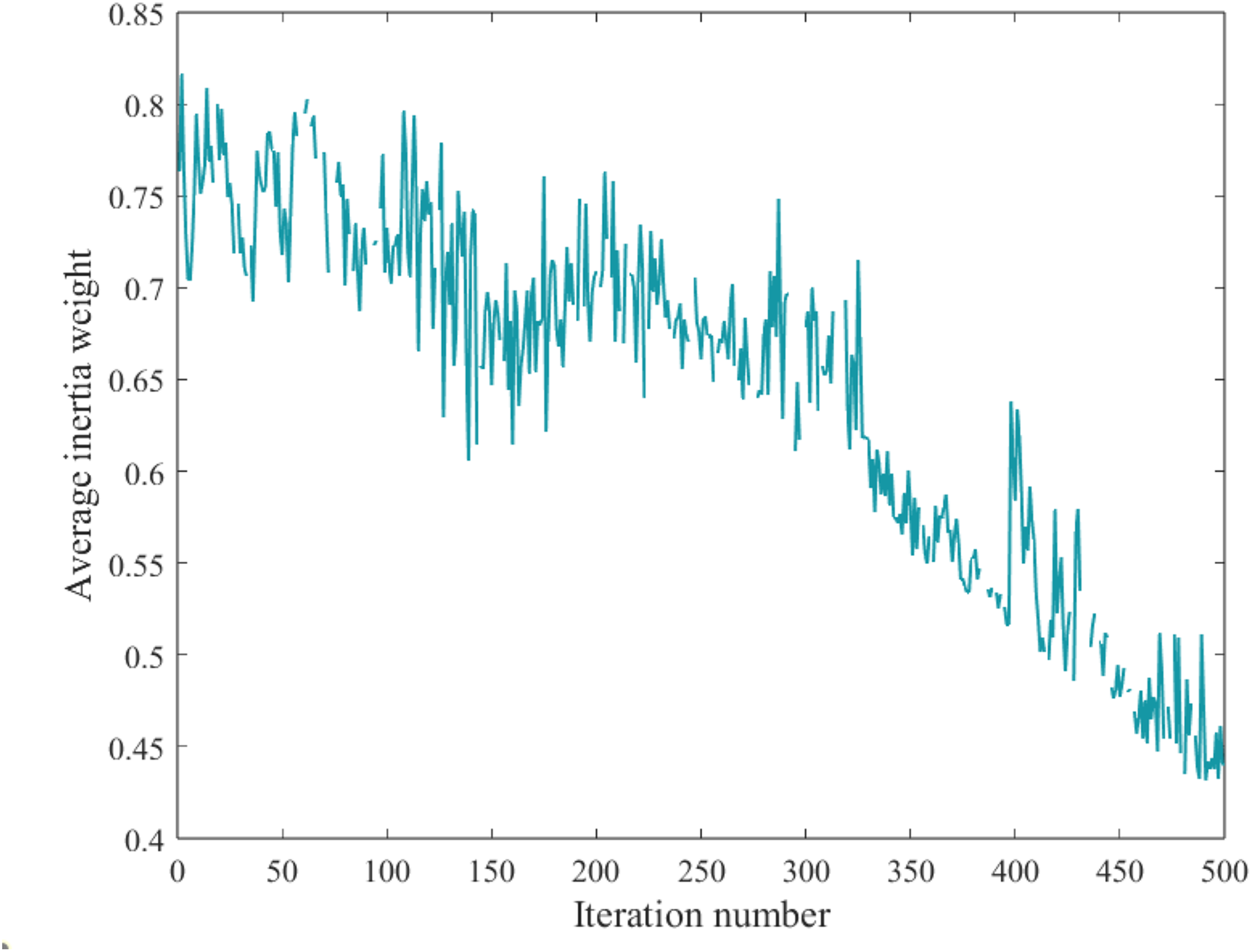
By observing the average inertia weight of all particles, it is evident that the average inertia weight adaptively decreases with the increasing number of iterations, as shown in Fig. 2.
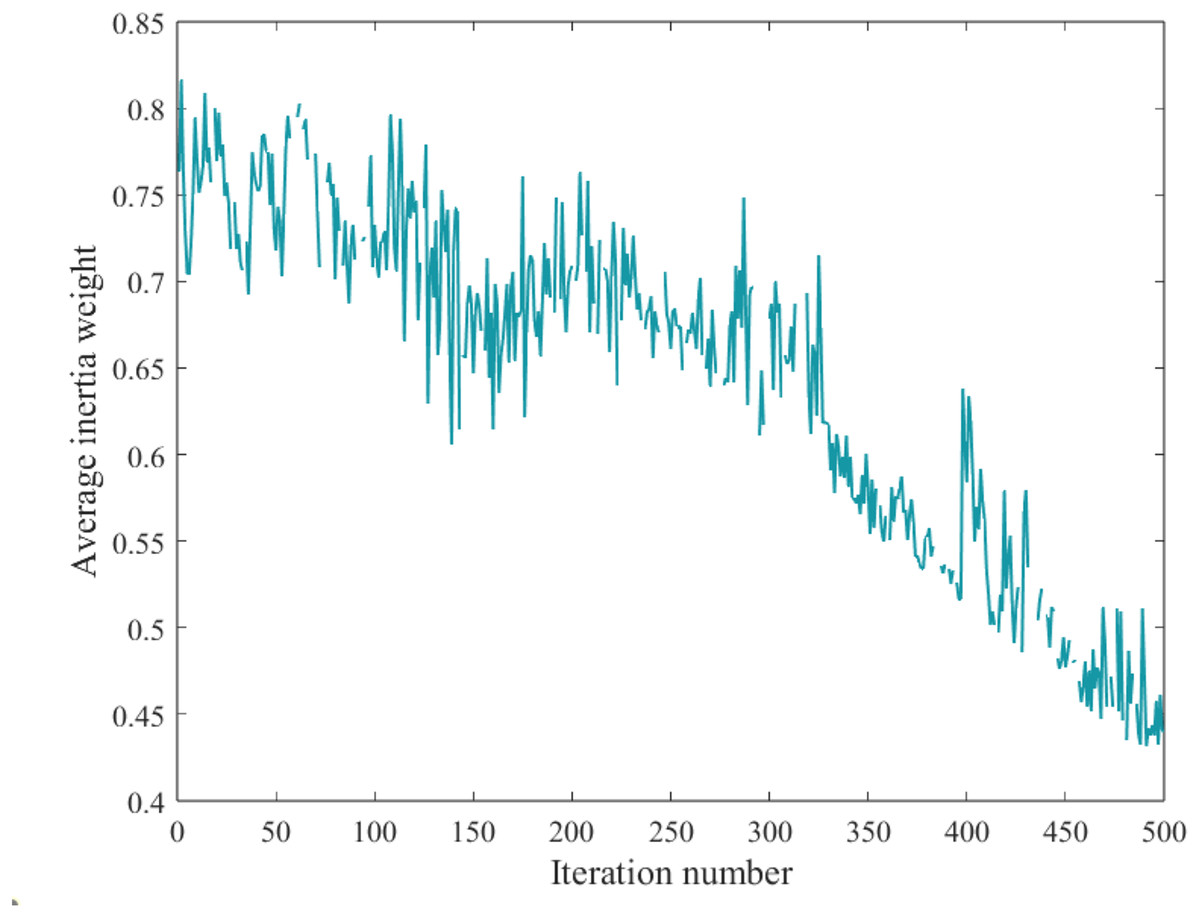
Figure 2: Evolution process of average inertia weight.
Different learning strategy for different sub-swarm
Best sub-swarm
Note that particles in the best sub-swarm tend to be relatively confident and believe that their learning mechanism is optimal. They update their positions based on their historical information. According to literature Xiong, Qiu & Liu (2020), sub-swarms are divided into two types of particles based on fitness values: optimal particles and non-optimal ordinary particles, and different learning strategies are assigned to each category. To prevent the best particles from falling into local optima, a random perturbation strategy is employed, as mentioned in Gou et al. (2017). Due to the effectiveness of Levy flight, a PSO that incorporates firefly behavior and Levy flight is introduced in Qiang, Hongwei & Shuzhi (2016), while Cui & Jin (2022) presents a grey wolf optimization algorithm based on Levy flight strategy. The Levy flight strategy enhances particle activity, expands the search range, and prevents the algorithm from being trapped in local optima. Additionally, to avoid meaningless position updates, a greedy strategy is introduced to determine whether to update the optimal particle’s position. In short, if the particle’s position updated using the Levy flight strategy is superior to the original position, the update is made. otherwise, the original position is retained. According to the operator for sub-swarm division in Eq. (3), particles with fitness values below a certain threshold are assigned to the S1 (best sub-swarm). By incorporating Levy flight and the greedy strategy into the best sub-swarm, PSO can avoid being trapped in local optima and address the loss of swarm diversity. Mathematically, the Levy flight strategy can be defined by Eq. (5):
(5) where:
represents the new optimal particle position after being updated by the Levy flight strategy. is the step-size scaling factor, typically set to 0.01. refers to the random path of the Levy flight, with . Both and follow a normal distribution, where and represent variances, and denotes the gamma function. To ensure better performance, the greedy strategy can be defined by Eq. (6):
(6) where, and represent the particle’s fitness values before and after being updated by the Levy flight strategy, respectively.
Better sub-swarm
In the better sub-swarm, the learning mechanism is used to acquire information from other sub-swarms to further enhance the information exchange between sub-swarms. In other words, to accelerate convergence process, the better sub-swarm must have the ability to integrate information from the best sub-swarm. A cooperative learning mechanism is employed in Niu et al. (2007) to obtain information from other sub-swarms. According to the operator defined in Eq. (3), particles with fitness values greater than or equal to f2 and less than f3 will be assigned to S2 (the better sub-swarm). Given the effectiveness of the cooperative learning strategy, the information from the optimal particles in the best sub-swarm is used in this study to enhance the swarm diversity and search capability. At the same time, the influence of the best particles in the better sub-swarm on other particles is reduced to accelerate population convergence. This learning strategy can be defined by Eq. (7):
(7) where, represents the optimal particle in the best sub-swarm (S1) in the j-th dimension during the t-th iteration. w is the adaptive inertia weight, and since the particles are in the better sub-swarm, the corresponding inertia weight rule is selected based on Eq. (2) to update the particle velocities.
Worse sub-swarm
To enhance the computational efficiency of the algorithm, the most commonly used optimization method is employed to update particle’s velocity in the worse sub-swarm. It is well known that learning factors play a crucial role in PSO. A fixed learning factor is proposed in Kennedy & Eberhart (1995) and has been widely adopted by many researchers. To better trade-off exploration and exploitation, a hybrid particle swarm optimization with sine cosine acceleration is introduced in Chen et al. (2018b), while sine and cosine learning factors are incorporated in Tang et al. (2021) for particles in the “hybrid domain” to accelerate the convergence process. According to the operator defined in Eq. (3), particles with fitness values greater than or equal to f3 and less than f4 are assigned to S3 (the worse sub-swarm). In view of this, the worse sub-swarm also utilizes sine and cosine learning factors to enhance the overall performance of the PSO. This learning strategy is defined by Eqs. (8)–(10):
(8)
(9)
(10) where denotes the cognitive learning factor, represents the social learning factor, and is a constant ( ).
Worst sub-swarm
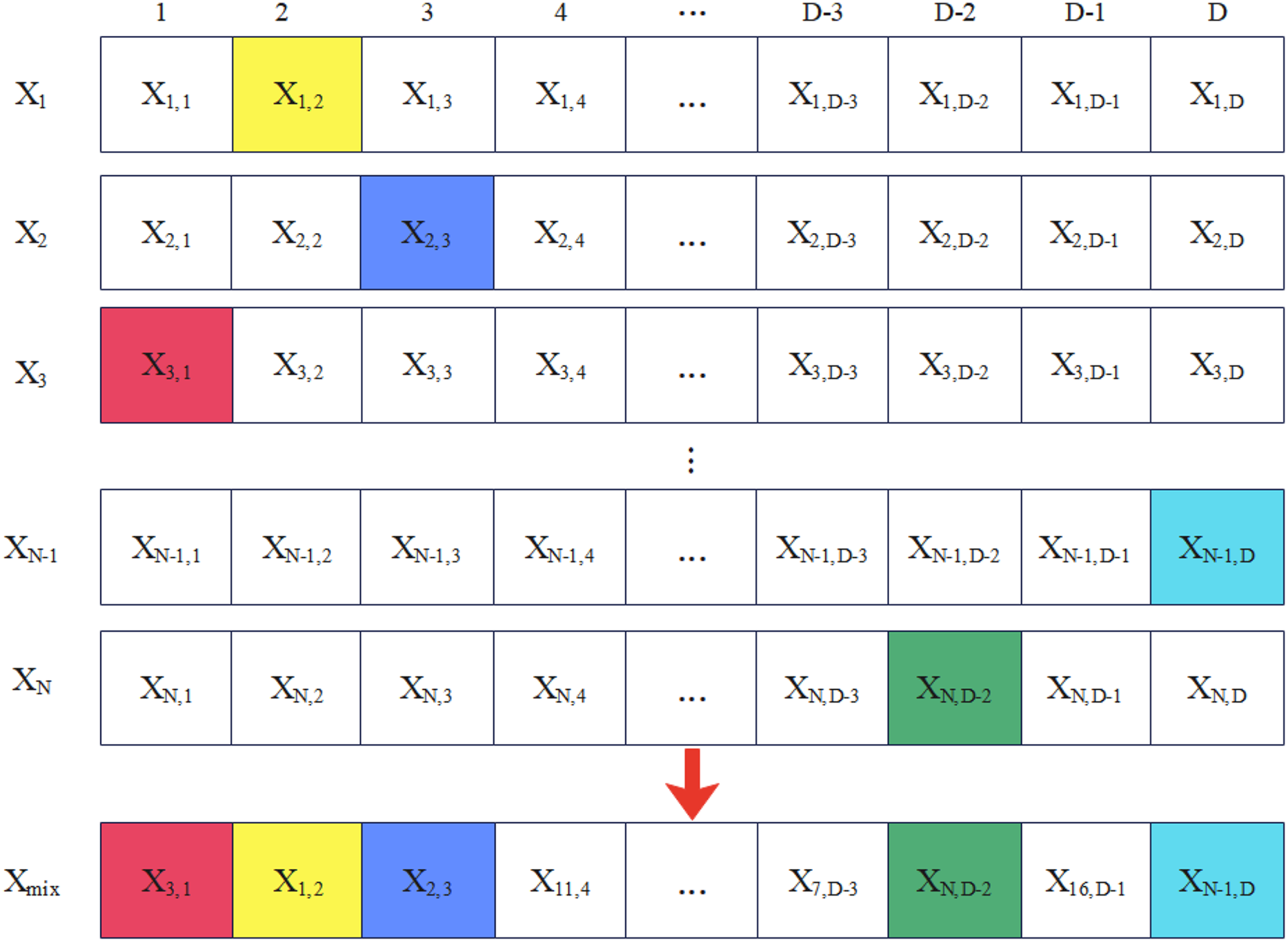
It is well known that the “cask effect” implies that the amount of water a cask can hold depends on its shortest plank rather than its longest. By extending the shortest plank and removing the limitation it creates, the cask’s water capacity can be increased. Hence, to strengthen the performance of the particles in the worst sub-swarm is particularly important for PSO. Particles in the worst sub-swarm are more likely to move in the wrong direction or get trapped in local optima. To deal with this issue, many strategies have been proposed to assist these particles evade local optima and find more promising solutions, such as Gaussian mutation, elite learning and random combination strategy, etc. In Yang & Li (2023b), Gaussian mutation is introduced to further update particles’ positions for the purpose of stopping them from falling into local optima. An elite learning strategy is proposed in Wang et al. (2021), and Xia et al. (2019) that allows particles to study from the best individuals in the best sub-swarm, thereby improving the convergence speed of the swarm. In addition, a random combination strategy is applied in Tang et al. (2021) to guide the velocity of particles in the “isolated domain” so as to increase the swarm diversity. As shown in Fig. 3, the random combination strategy can reconstruct each dimension of the particle Xmix, where each dimension is randomly selected from the best historical positions of different particles in order to ensure multiple dimensions are not selected from the same particle.
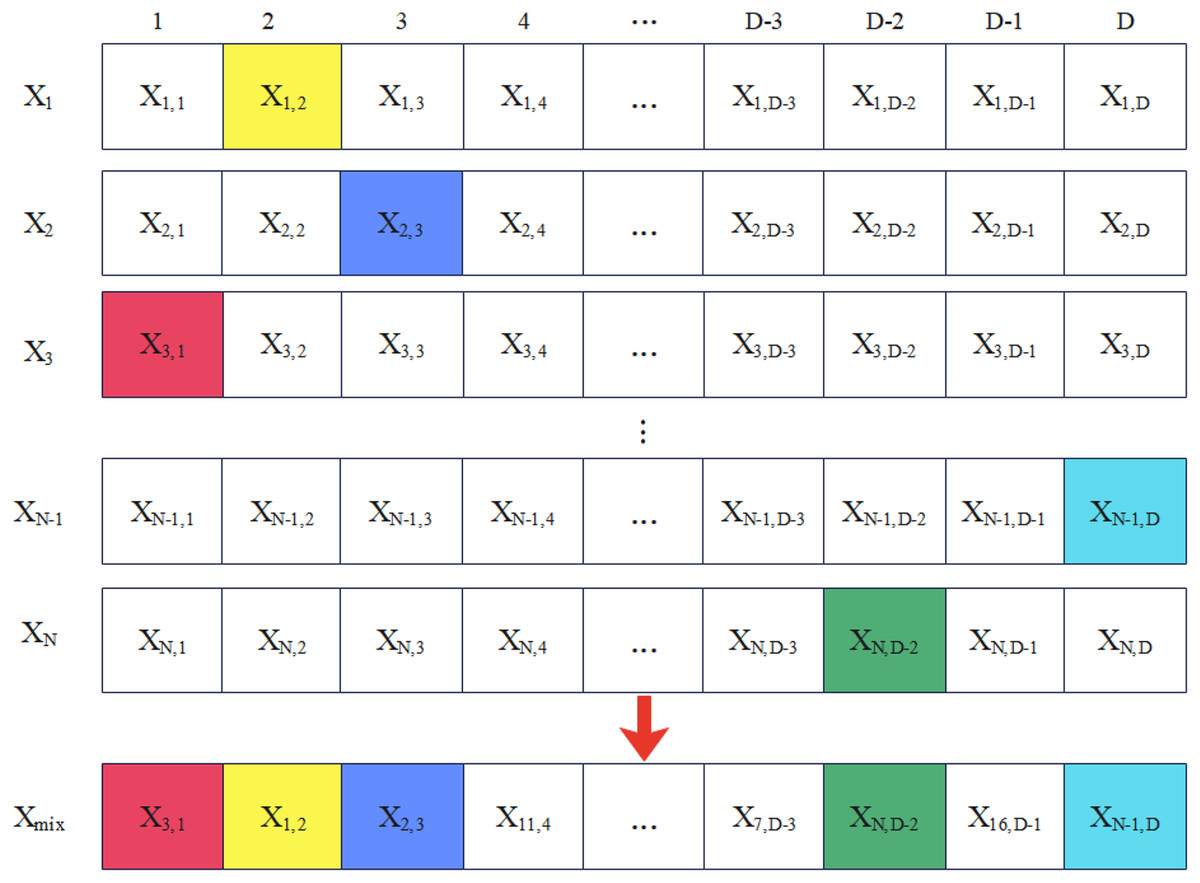
Figure 3: The process of random combination.
According to the operator described in Eq. (3), particles with fitness values greater than or equal to f4 are assigned to S4 (the worst sub-swarm). In the worst sub-swarm, particles update their velocities using elite learning and random combination strategies. Additionally, Gaussian mutation is adaptively introduced to further update particle’s position and avoid local optima. The learning strategy can be defined by Eqs. (11)–(13):
(11)
(12)
(13) where Xmix,j represents the particle reconstructed in the j-th dimension, and w is the adaptive inertia weight. Since the particle is in the worst sub-swarm, wmax is selected according to Eq. (2) to update the particle’s velocity. r is a random number between 0 and 1 that is used to determine whether a Gaussian mutation should be triggered, x stands for the current particle’s position, and randn denotes a Gaussian-distributed random number with mean of 0 and variance of 1. The new position calculated by GV(x) replaces or influences the particle’s current position x to increase population diversity and avoid local optima. When the condition in Eq. (12) is met, Gaussian mutation will be trigged to help the particles search for better solutions.
BFGS quasi-newton method
The Quasi-Newton method is a classic numerical technique used to solve unconstrained optimization problems, which is developed to avoid directly calculating the Hessian matrix, making it an efficient method for solving large-scale optimization problems. The BFGS (Broyden, 1970; Fletcher, 1970; Goldfarb, 1970; Shanno, 1970) method is one of the most widely used Quasi-Newton methods. It begins by constructing an inverse matrix approximating the Hessian, and then updates this matrix using gradient information. This update is performed according to the BFGS formula, progressively approximating the true Hessian matrix, thus obtaining a better search direction in each iteration.
To address the slow convergence problem of DMS-PSO, a local search phase using the BFGS Quasi-Newton method is added to the algorithm in Zhao et al. (2008), enhancing the local search capability of particles. The Quasi-Newton Method constructs a local quadratic model to approximate the objective function by updating the Hessian matrix approximation. The quadratic model generally takes the form of Eq. (14):
(14) where mk(p) is the quadratic approximation model of the objective function at , p is the search direction vector, and Bk is the Hessian matrix at xk that is a positive definite and symmetric matrix.
Based on this quadratic model, the Quasi-Newton method can determine the search direction at each step, which is calculated by Eq. (15):
(15)
This direction ensures the fastest decrease in the quadratic model, thus accelerating convergence to the minimum of the objective function. If x* is the optimal solution of the quadratic model, then x* must satisfy: .
The Quasi-Newton method updates the Hessian matrix approximation at each iteration. The most commonly used update formula is the BFGS formula, which ensures that the matrix remains symmetric and positive definite, preserving the validity of the quadratic model. The update formula for the approximate Hessian matrix can be described by Eq. (16):
(16) where , , with B0 being the identity matrix.
The BFGS Quasi-Newton method is employed to refine the optimal solution obtained, thereby enhancing the local search capability. It is worth noting that a random number between 0 and 1 is generated to determine whether the IDSMPSO will use the Quasi-Newton method or not. When the random number is less than or equal to a pre-set threshold, the algorithm updates each sub-swarm based on different learning mechanisms, otherwise, the Quasi-Newton method is executed. Extensive experiments have demonstrated that setting the threshold to 0.9 yields the best results. As described above, the pseudocode of IDSMPSO is outlined in Algorithm 1.
| Input: Setup Parameters: size of the whole population: N, max iterations: T_Max, Inertia weight: wmin = 0.4 and wmax = 0.9, learning factor c1, c2, c3, Levy Flight Parameters: β = 3/2, α = 0.01, the dimension: D, velocity boundary: [v_min, v_max], position boundary: [x_min, x_max]. |
| Process: |
| 1. Initialize Position X, Velocity V and Fitness value (f) for N individuals |
| 2. Initialize Pbest, Gbest, fPbest, fGbest: |
| 3. Pbest=X |
| 4. fPbest=f |
| 5. [fmin,ind]=min(f) |
| 6. fGbest=fmin |
| 7. Gbest=Xind |
| 8. Update the sub-swarm size and division of sub-swarm according to Eq. (3) |
| 9. for i=1 to T_Max do |
| 10. R1=rand |
| 11. if R1<= tpre-set then |
| 12. for j=1 to N do |
| 13. Updating adaptive inertia weights according to Eq. (4) |
| 14. if particles j belong to the best sub-swarm then |
| 15. Update Vj by Eq. (1) and check velocity boundary |
| 16. Update Xj by Eq. (2) and check position boundary |
| 17. Use Levy Flight and greedy algorithm to handle X by Eqs. (5), (6) |
| 18. Calculating f |
| 19. else if particles j belong to the better sub-swarm then |
| 20. Update Vj by Eq. (7) and check velocity boundary |
| 21. Update Xj by Eq. (2) and check position boundary |
| 22. Calculating f |
| 23. else if particles j belong to the worse sub-swarm |
| 24. Update Vj by Eq. (10) and check velocity boundary |
| 25. Update Xj by Eq. (2) and check position boundary |
| 26. Calculating f |
| 27. else particles j belong to the worst sub-swarm |
| 28. Update Vj by Eq. (11) and check velocity boundary |
| 29. Update Xj by Eqs. (2), (12), (13) and check position boundary |
| 30. Calculating f |
| 31. end if |
| 32. end for |
| 33. else |
| 34. Using the BFGS Newton method to handle X |
| 35. end if |
| 36. Reupdate the sub-swarm size and division of sub-swarm according to Eq. (3) |
| 37. for j=1 to N do |
| 38. Update Pbest, fPbest, Gbest, fGbest |
| 39. end for |
| 40. end for |
| Output: GBest |
Experiments and analysis
Test functions
To demonstrate the performance of IDSMPSO in unimodal, multimodal and complex scenarios, the CEC’17 and CEC’22 benchmark test suites are selected. CEC’17 consists of 29 functions (f2 is excluded due to its instability in high-dimensional cases), including unimodal (f1, f3), multimodal (f4–f10), hybrid (f11–f20), and composition (f21–f30) functions. The search range for each function is shown in Table 1. Moreover, Table 2 presents the CEC’22 test suite. Specifically, within the test suite, f1 belongs to the unimodal category, while f2 to f5 are classified as multimodal functions, f6 to f8 fall into the hybrid function category, and f9 to f12 are defined as composite functions, each variable is constrained within the range of [−100, 100].
| Type | No | Function | F(x*) | Search area |
|---|---|---|---|---|
| Unimodal | 1 | Shifted and rotated Bent Cigar function | 100 | [−100, 100]D |
| 3 | Shifted and rotated Zakharov function | 300 | ||
| Multimodal | 4 | Shifted and rotated Rosenbrock’s function | 400 | |
| 5 | Shifted and rotated Rastrigin’s function | 500 | ||
| 6 | Shifted and rotated expanded Scaffer’s function | 600 | ||
| 7 | Shifted and rotated Lunacek Bi-Rastrigin function | 700 | ||
| 8 | Shifted and rotated non-continuous Rastrigin’s function | 800 | ||
| 9 | Shifted and rotated Levy function | 900 | ||
| 10 | Shifted and rotated Schwefel’s function | 1,000 | ||
| Hybrid | 11 | Hybrid function 1 (N = 3) | 1,100 | |
| 12 | Hybrid function 2 (N = 3) | 1,200 | ||
| 13 | Hybrid function 3 (N = 3) | 1,300 | ||
| 14 | Hybrid function 4 (N = 4) | 1,400 | ||
| 15 | Hybrid function 5 (N = 4) | 1,500 | ||
| 16 | Hybrid function 6 (N = 4) | 1,600 | ||
| 17 | Hybrid function 6 (N = 5) | 1,700 | ||
| 18 | Hybrid function 6 (N = 5) | 1,800 | ||
| 19 | Hybrid function 6 (N = 5) | 1,900 | ||
| 20 | Hybrid function 6 (N = 6) | 2,000 | ||
| Composition | 21 | Composition function 1 (N = 3) | 2,100 | |
| 22 | Composition function 2 (N = 3) | 2,200 | ||
| 23 | Composition function 3 (N = 4) | 2,300 | ||
| 24 | Composition function 4 (N = 4) | 2,400 | ||
| 25 | Composition function 5 (N = 5) | 2,500 | ||
| 26 | Composition function 6 (N = 5) | 2,600 | ||
| 27 | Composition function 7 (N = 6) | 2,700 | ||
| 28 | Composition function 8 (N = 6) | 2,800 | ||
| 29 | Composition function 9 (N = 3) | 2,900 | ||
| 30 | Composition function 10 (N = 3) | 3,000 |
Note:
x*, global optimum; D, dimension.
| Type | No | Function | F(x*) | Search area |
|---|---|---|---|---|
| Unimodal | 1 | Shifted and full rotated Zakharov function | 300 | [−100, 100]D |
| Multimodal | 2 | Shifted and full rotated Rosenbrock’s function | 400 | |
| 3 | Shifted and full rotated expanded Schaffer’s f6 function | 600 | ||
| 4 | Shifted and full rotated non-continuous Rastrigin’s function | 800 | ||
| 5 | Shifted and full rotated Levy function | 900 | ||
| Hybrid | 6 | Hybrid function 1 (N = 3) | 1,800 | |
| 7 | Hybrid function 2 (N = 6) | 2,000 | ||
| 8 | Hybrid function 3 (N = 5) | 2,200 | ||
| Composition | 9 | Composition function 1 (N = 5) | 2,300 | |
| 10 | Composition function 2 (N = 4) | 2,400 | ||
| 11 | Composition function 3 (N = 5) | 2,600 | ||
| 12 | Composition function 4 (N = 6) | 2,700 |
Note:
x*, global optimum; D, dimension.
Parameter settings
To evaluate the performance of our proposal, eight competitive algorithms are selected for comparison, including four state-of-the-art optimizers (Grey Wolf Optimizer (GWO) (Mirjalili, Mirjalili & Lewis, 2014), GOOSE Algorithm (GO) (Hamad & Rashid, 2024), Equilibrium Optimizer (EO) (Faramarzi et al., 2020), Kepler Optimization Algorithm (KOA) (Abdel-Basset et al., 2023)) and four classical PSO variants (MPSO (Liu, Zhang & Tu, 2020), EAPSO (Zhang, 2023), HPSOALS (Wang et al., 2024), DMPSORH (Tang et al., 2021)). To ensure a fair evaluation, the parameter settings of all the comparison algorithms are adopted from their original studies, with the main configurations summarized in Table 3. The parameters of IDSMPSO are as follows: wmax is set to 0.9 and wmin is set to 0.4 so as to strengthen the convergence rate of particles in the worst sub-swarm. As the number of iterations increases, w is adaptively adjusted based on the particle’s state. For the Levy flight strategy, β = 3/2 and α = 0.01 (step-size factor). The maximum number of population iterations (T_Max) is set to 1,000 and the swarm size N is set to 30. Each test is repeated independently 30 times to minimize statistical errors. Additionally, to prevent particles from moving beyond the boundary, IDSMPSO includes boundary handling mechanisms. If a particle’s position exceeds the predefined maximum value, its position is reassigned to the previous maximum. Likewise, if the position of a particle is less than the minimum value, it is reset to the previous minimum. The same boundary handling method is applied to the particle’s velocity.
| Peer algorithms | Parameter setting | Ref. |
|---|---|---|
| GWO | a: 2~0, r1: 0~1, r2: 0~1, C: 0~2, A: −2~2 | Mirjalili, Mirjalili & Lewis (2014) |
| GO | pro: 0~1, coe: 0~1, S_W: 5~25, α: 0~2, rnd: 0~1. | Hamad & Rashid (2024) |
| EO | a1: 2, a2: 1, GP: 0.5, Ceq: 5, λ: 0~1. | Faramarzi et al. (2020) |
| KOA | w: 0.5~0.9, γ0: 1.0, k: 2~5 | Abdel-Basset et al. (2023) |
| MPSO | w: 0.9~0.4, c1 = c2 = 2, vmax: 10 | Liu, Zhang & Tu (2020) |
| EAPSO | w: 1.0~0.01, c1: 1.0~0.01, c2: 1.0~0.01. | Zhang (2023) |
| HPSOALS | w: 0.9~0.4, c1 = c2 = c3 = 1.5, v: −10~10. | Wang et al. (2024) |
| DMPSORH | w: 0.8~0.4, c1: 1, c2: 1.2, c3: 0.3, vmax: 10, OR: 0.2. | Tang et al. (2021) |
| IDSMPSO | w: 0.9~0.4, c1 = c2 = c3 = 1.49445, β: 3/2, α: 0.01. | / |
Comparison on CEC’17 test suite
In this section, experiments are conducted on the CEC’17 with three different dimensions (D = 30, 50, 100). Without loss of generality, the metrics including the mean value (mv), standard deviation value (sdv), rank value (rv), average rank (AR) and final rank (FR) of the best results achieved are used to evaluate the peer algorithms. Tables 4–6 report the experimental results, and the mean value (mv), standard deviation value (sdv), rank value (rv), average rank (AR) and final rank (FR) of the best results are highlighted in bold.
| Func | Metric | GWO | GO | EO | KOA | MPSO | EAPSO | HPSOALS | DMPSORH | IDSMPSO |
|---|---|---|---|---|---|---|---|---|---|---|
| f1 | mv | 8.758E+10 | 6.462E+03 | 3.584E+10 | 1.127E+10 | 5.188E+07 | 3.953E+09 | 1.992E+10 | 1.135E+07 | 1.156E+02 |
| sdv | 1.167E+10 | 1.998E+03 | 7.030E+09 | 3.879E+09 | 8.799E+07 | 8.009E+08 | 5.929E+09 | 7.969E+06 | 8.314E+01 | |
| rv | 9 | 2 | 8 | 6 | 4 | 5 | 7 | 3 | 1 | |
| f3 | mv | 1.552E+05 | 5.257E+04 | 1.633E+05 | 1.966E+05 | 1.349E+04 | 1.454E+05 | 9.092E+04 | 1.457E+04 | 3.000E+00 |
| sdv | 1.855E+05 | 2.921E+04 | 6.551E+04 | 4.691E+04 | 5.876E+03 | 3.278E+04 | 3.176E+04 | 9.580E+03 | 0.000E+00 | |
| rv | 7 | 4 | 8 | 9 | 2 | 6 | 5 | 3 | 1 | |
| f4 | mv | 8.809E+03 | 5.089E+02 | 8.554E+03 | 2.166E+03 | 5.147E+02 | 7.880E+02 | 4.167E+03 | 5.351E+02 | 4.026E+02 |
| sdv | 3.487E+03 | 1.141E+01 | 2.702E+03 | 5.184E+02 | 4.701E+01 | 8.395E+01 | 1.699E+03 | 2.402E+01 | 1.910E+00 | |
| rv | 9 | 2 | 8 | 6 | 3 | 5 | 7 | 4 | 1 | |
| f5 | mv | 8.709E+02 | 7.990E+02 | 8.446E+02 | 8.207E+02 | 5.819E+02 | 7.579E+02 | 7.540E+02 | 7.088E+02 | 7.190E+02 |
| sdv | 5.155E+01 | 1.501E+01 | 4.847E+01 | 2.681E+01 | 2.125E+01 | 2.403E+01 | 3.146E+01 | 4.168E+01 | 4.844E+01 | |
| rv | 9 | 6 | 8 | 7 | 1 | 5 | 4 | 2 | 3 | |
| f6 | mv | 6.687E+02 | 6.658E+02 | 6.778E+02 | 6.558E+02 | 6.080E+02 | 6.413E+02 | 6.596E+02 | 6.557E+02 | 6.546E+02 |
| sdv | 1.169E+01 | 3.050E+00 | 1.057E+01 | 1.191E+01 | 4.810E+00 | 1.389E+01 | 7.750E+00 | 7.430E+00 | 1.397E+01 | |
| rv | 8 | 5 | 9 | 5 | 1 | 2 | 7 | 4 | 3 | |
| f7 | mv | 1.374E+03 | 1.327E+03 | 1.346E+03 | 1.230E+03 | 8.148E+02 | 1.109E+03 | 1.128E+03 | 1.165E+03 | 1.140E+03 |
| sdv | 9.910E+01 | 2.433E+01 | 7.184E+01 | 5.990E+01 | 3.137E+01 | 4.197E+01 | 6.722E+01 | 1.030E+02 | 8.545E+01 | |
| rv | 9 | 7 | 8 | 6 | 1 | 2 | 3 | 5 | 4 | |
| f8 | mv | 1.110E+03 | 1.013E+03 | 1.095E+03 | 1.106E+03 | 8.655E+02 | 1.059E+03 | 1.008E+03 | 9.452E+02 | 9.600E+02 |
| sdv | 2.970E+01 | 8.930E+00 | 3.271E+01 | 2.352E+01 | 1.649E+01 | 2.341E+01 | 3.203E+01 | 2.735E+01 | 3.714E+01 | |
| rv | 9 | 5 | 7 | 8 | 1 | 6 | 4 | 2 | 3 | |
| f9 | mv | 8.692E+03 | 5.554E+03 | 9.242E+03 | 9.417E+03 | 1.175E+03 | 4.599E+03 | 5.378E+03 | 4.942E+03 | 4.350E+03 |
| sdv | 1.867E+03 | 1.236E+02 | 1.863E+03 | 2.731E+03 | 2.753E+02 | 3.048E+03 | 1.109E+03 | 1.032E+03 | 1.723E+03 | |
| rv | 7 | 6 | 8 | 9 | 1 | 3 | 5 | 4 | 2 | |
| f10 | mv | 8.581E+03 | 5.568E+03 | 8.066E+03 | 9.392E+03 | 4.584E+03 | 8.683E+03 | 7.015E+03 | 7.904E+03 | 4.539E+03 |
| sdv | 5.687E+02 | 6.798E+02 | 6.274E+02 | 3.981E+02 | 7.051E+02 | 3.454E+02 | 5.860E+02 | 1.023E+03 | 6.104E+02 | |
| rv | 7 | 3 | 6 | 9 | 2 | 8 | 4 | 5 | 1 | |
| f11 | mv | 2.386E+04 | 1.337E+03 | 6.436E+03 | 8.047E+03 | 1.217E+03 | 3.584E+03 | 3.147E+03 | 1.255E+03 | 1.207E+03 |
| sdv | 3.097E+04 | 6.313E+01 | 2.227E+03 | 2.112E+03 | 3.863E+01 | 2.005E+03 | 1.008E+03 | 3.900E+01 | 3.685E+01 | |
| rv | 9 | 4 | 7 | 8 | 2 | 6 | 5 | 3 | 1 | |
| f12 | mv | 6.315E+09 | 2.894E+06 | 5.780E+09 | 8.515E+08 | 1.210E+06 | 3.245E+08 | 2.471E+09 | 2.106E+06 | 2.534E+03 |
| sdv | 3.310E+09 | 1.486E+06 | 2.353E+09 | 3.435E+08 | 1.482E+06 | 1.157E+08 | 1.228E+09 | 1.923E+06 | 4.144E+02 | |
| rv | 9 | 4 | 8 | 6 | 2 | 5 | 7 | 3 | 1 | |
| f13 | mv | 1.783E+09 | 8.395E+04 | 1.116E+09 | 1.892E+08 | 1.582E+04 | 1.116E+08 | 8.078E+08 | 3.154E+04 | 2.765E+03 |
| sdv | 2.221E+09 | 6.306E+04 | 8.895E+08 | 9.955E+07 | 1.433E+04 | 5.978E+07 | 1.351E+09 | 1.772E+04 | 4.394E+02 | |
| rv | 9 | 4 | 8 | 6 | 2 | 5 | 7 | 3 | 1 | |
| f14 | mv | 1.324E+07 | 2.968E+04 | 2.506E+06 | 1.666E+06 | 6.073E+03 | 6.851E+05 | 4.710E+05 | 1.482E+04 | 1.531E+03 |
| sdv | 3.725E+07 | 2.870E+04 | 2.040E+06 | 1.523E+06 | 6.652E+03 | 4.828E+05 | 9.378E+05 | 3.338E+04 | 2.955E+01 | |
| rv | 9 | 4 | 8 | 7 | 2 | 6 | 5 | 3 | 1 | |
| f15 | mv | 3.237E+08 | 2.418E+04 | 3.126E+07 | 2.243E+07 | 2.869E+03 | 1.540E+07 | 1.846E+05 | 9.207E+03 | 1.870E+03 |
| sdv | 9.647E+08 | 2.369E+04 | 7.803E+07 | 2.155E+07 | 1.551E+03 | 1.297E+07 | 7.217E+05 | 7.488E+03 | 7.260E+02 | |
| rv | 9 | 4 | 8 | 7 | 2 | 6 | 5 | 3 | 1 | |
| f16 | mv | 4.990E+03 | 3.760E+03 | 4.440E+03 | 4.207E+03 | 2.551E+03 | 3.559E+03 | 3.856E+03 | 3.257E+03 | 2.926E+03 |
| sdv | 7.643E+02 | 4.832E+02 | 8.592E+02 | 3.075E+02 | 2.883E+02 | 2.695E+02 | 3.625E+02 | 2.684E+02 | 3.314E+02 | |
| rv | 9 | 5 | 8 | 7 | 1 | 4 | 6 | 3 | 2 | |
| f17 | mv | 3.278E+03 | 2.806E+03 | 3.086E+03 | 2.880E+03 | 2.055E+03 | 2.534E+03 | 2.575E+03 | 2.579E+03 | 2.001E+03 |
| sdv | 8.461E+02 | 3.786E+02 | 7.121E+02 | 1.692E+02 | 2.032E+02 | 1.351E+02 | 2.812E+02 | 2.317E+02 | 1.857E+02 | |
| rv | 9 | 6 | 8 | 7 | 2 | 3 | 4 | 5 | 1 | |
| f18 | mv | 8.659E+07 | 4.588E+05 | 1.975E+07 | 2.575E+07 | 1.404E+05 | 8.062E+06 | 2.739E+06 | 1.530E+05 | 1.975E+03 |
| sdv | 1.278E+08 | 3.057E+05 | 2.326E+07 | 1.573E+07 | 1.169E+05 | 7.197E+06 | 4.659E+06 | 1.436E+05 | 5.125E+01 | |
| rv | 9 | 4 | 7 | 8 | 2 | 6 | 5 | 3 | 1 | |
| f19 | mv | 3.235E+07 | 5.081E+05 | 5.649E+07 | 3.574E+07 | 5.672E+03 | 2.637E+07 | 8.323E+06 | 7.997E+03 | 2.227E+03 |
| sdv | 8.561E+07 | 1.665E+05 | 6.889E+07 | 2.372E+07 | 3.060E+03 | 2.115E+07 | 1.797E+07 | 6.274E+03 | 2.628E+02 | |
| rv | 7 | 4 | 9 | 8 | 2 | 6 | 5 | 3 | 1 | |
| f20 | mv | 2.962E+03 | 3.131E+03 | 2.941E+03 | 3.176E+03 | 2.335E+03 | 2.830E+03 | 2.745E+03 | 2.958E+03 | 2.323E+03 |
| sdv | 2.071E+02 | 2.451E+02 | 1.968E+02 | 1.809E+02 | 1.837E+02 | 1.574E+02 | 2.245E+02 | 2.507E+02 | 1.553E+02 | |
| rv | 7 | 8 | 5 | 9 | 2 | 4 | 3 | 6 | 1 | |
| f21 | mv | 2.619E+03 | 2.671E+03 | 2.652E+03 | 2.604E+03 | 2.367E+03 | 2.540E+03 | 2.569E+03 | 2.544E+03 | 2.549E+03 |
| sdv | 5.722E+01 | 5.658E+01 | 5.407E+01 | 2.766E+01 | 2.228E+01 | 2.143E+01 | 4.376E+01 | 4.211E+01 | 7.096E+01 | |
| rv | 7 | 9 | 8 | 6 | 1 | 2 | 5 | 3 | 4 | |
| f22 | mv | 9.185E+03 | 7.746E+03 | 9.053E+03 | 7.404E+03 | 2.461E+03 | 4.240E+03 | 8.153E+03 | 7.973E+03 | 5.430E+03 |
| sdv | 1.311E+03 | 5.941E+02 | 1.118E+03 | 2.497E+03 | 7.917E+02 | 2.728E+03 | 8.111E+02 | 2.026E+03 | 1.680E+03 | |
| rv | 9 | 5 | 8 | 4 | 1 | 2 | 7 | 6 | 3 | |
| f23 | mv | 3.387E+03 | 3.512E+03 | 3.347E+03 | 3.013E+03 | 2.745E+03 | 2.909E+03 | 3.436E+03 | 3.462E+03 | 2.722E+03 |
| sdv | 1.420E+02 | 1.772E+02 | 1.963E+02 | 3.257E+01 | 3.879E+01 | 2.766E+01 | 1.685E+02 | 1.644E+02 | 1.053E+02 | |
| rv | 6 | 9 | 5 | 4 | 2 | 3 | 7 | 8 | 1 | |
| f24 | mv | 3.513E+03 | 3.691E+03 | 3.501E+03 | 3.175E+03 | 2.922E+03 | 2.872E+03 | 3.573E+03 | 3.450E+03 | 3.267E+03 |
| sdv | 1.578E+02 | 1.353E+02 | 2.000E+02 | 4.422E+01 | 3.294E+01 | 4.106E+01 | 1.171E+02 | 1.231E+02 | 1.072E+02 | |
| rv | 7 | 9 | 6 | 3 | 2 | 1 | 8 | 5 | 4 | |
| f25 | mv | 4.628E+03 | 2.920E+03 | 4.071E+03 | 3.533E+03 | 2.928E+03 | 3.189E+03 | 3.544E+03 | 2.917E+03 | 2.887E+03 |
| sdv | 5.155E+02 | 1.640E+01 | 3.558E+02 | 2.049E+02 | 2.813E+01 | 7.680E+01 | 2.581E+02 | 2.092E+01 | 1.935E+01 | |
| rv | 9 | 2 | 8 | 6 | 4 | 5 | 7 | 3 | 1 | |
| f26 | mv | 1.028E+04 | 8.041E+03 | 1.002E+04 | 7.264E+03 | 5.220E+03 | 5.163E+03 | 8.792E+03 | 8.358E+03 | 5.069E+03 |
| sdv | 1.373E+03 | 2.213E+03 | 9.789E+02 | 3.189E+02 | 1.331E+03 | 1.100E+03 | 7.270E+02 | 1.049E+03 | 1.931E+03 | |
| rv | 9 | 5 | 8 | 4 | 3 | 2 | 7 | 6 | 1 | |
| f27 | mv | 4.066E+03 | 4.206E+03 | 3.948E+03 | 3.450E+03 | 3.548E+03 | 3.215E+03 | 4.045E+03 | 4.224E+03 | 3.486E+03 |
| sdv | 3.628E+02 | 3.895E+02 | 2.753E+02 | 5.172E+01 | 2.690E+01 | 2.156E+01 | 2.514E+02 | 3.263E+02 | 1.104E+02 | |
| rv | 7 | 8 | 5 | 2 | 4 | 1 | 6 | 9 | 3 | |
| f28 | mv | 6.927E+03 | 3.222E+03 | 5.767E+03 | 4.488E+03 | 3.333E+03 | 3.511E+03 | 4.974E+03 | 3.295E+03 | 3.120E+03 |
| sdv | 1.257E+03 | 1.411E+01 | 5.996E+02 | 4.796E+02 | 7.269E+01 | 6.688E+01 | 5.484E+02 | 3.290E+01 | 4.202E+01 | |
| rv | 9 | 2 | 8 | 6 | 4 | 5 | 7 | 3 | 1 | |
| f29 | mv | 7.379E+03 | 5.115E+03 | 6.336E+03 | 5.359E+03 | 3.709E+03 | 4.816E+03 | 5.363E+03 | 4.710E+03 | 3.795E+03 |
| sdv | 2.048E+03 | 4.686E+02 | 1.113E+03 | 4.179E+02 | 2.384E+02 | 3.153E+02 | 5.455E+02 | 3.945E+02 | 2.435E+02 | |
| rv | 9 | 5 | 8 | 6 | 1 | 4 | 7 | 3 | 2 | |
| f30 | mv | 8.989E+08 | 2.115E+06 | 1.565E+08 | 3.889E+07 | 9.808E+03 | 2.269E+07 | 5.894E+07 | 2.082E+05 | 8.495E+03 |
| sdv | 9.870E+08 | 1.542E+06 | 1.440E+08 | 1.835E+07 | 4.950E+03 | 1.775E+07 | 6.484E+07 | 2.311E+05 | 3.135E+03 | |
| rv | 9 | 4 | 8 | 6 | 2 | 5 | 7 | 3 | 1 | |
| AR | 8.31 | 5.00 | 7.51 | 6.37 | 2.03 | 4.24 | 5.72 | 4.00 | 1.75 | |
| FR | 9 | 5 | 8 | 7 | 2 | 4 | 6 | 3 | 1 | |
| Func | Metric | GWO | GO | EO | KOA | MPSO | EAPSO | HPSOALS | DMPSORH | IDSMPSO |
|---|---|---|---|---|---|---|---|---|---|---|
| f1 | mv | 4.714E+10 | 6.251E+03 | 3.110E+10 | 1.187E+10 | 8.862E+07 | 3.923E+09 | 2.184E+10 | 8.987E+06 | 1.508E+02 |
| sdv | 8.759E+09 | 1.765E+03 | 5.509E+09 | 4.191E+09 | 1.896E+08 | 6.811E+08 | 4.725E+09 | 1.058E+07 | 1.743E+02 | |
| rv | 9 | 2 | 8 | 6 | 4 | 5 | 7 | 3 | 1 | |
| f3 | mv | 1.571E+05 | 2.290E+05 | 2.113E+05 | 3.899E+05 | 8.251E+04 | 2.999E+05 | 1.659E+05 | 8.421E+04 | 3.000E+02 |
| sdv | 2.667E+04 | 5.766E+04 | 4.865E+04 | 7.886E+04 | 2.274E+04 | 5.500E+04 | 3.452E+04 | 2.409E+04 | 0.000E+00 | |
| rv | 4 | 7 | 6 | 9 | 2 | 8 | 5 | 3 | 1 | |
| f4 | mv | 3.087E+04 | 5.598E+02 | 2.303E+04 | 8.558E+03 | 8.459E+02 | 1.928E+03 | 1.498E+04 | 8.170E+02 | 4.005E+02 |
| sdv | 6.213E+03 | 3.286E+01 | 5.121E+03 | 2.180E+03 | 2.252E+02 | 3.786E+02 | 4.085E+03 | 8.899E+01 | 1.380E+00 | |
| rv | 9 | 2 | 8 | 6 | 4 | 5 | 7 | 3 | 1 | |
| f5 | mv | 1.146E+03 | 8.868E+02 | 1.136E+03 | 1.132E+03 | 6.912E+02 | 1.055E+03 | 9.998E+02 | 8.275E+02 | 1.032E+03 |
| sdv | 3.587E+01 | 1.900E+01 | 4.812E+01 | 5.001E+01 | 4.246E+01 | 6.194E+01 | 5.316E+01 | 3.760E+01 | 1.296E+02 | |
| rv | 9 | 3 | 8 | 7 | 1 | 6 | 4 | 2 | 5 | |
| f6 | mv | 6.934E+02 | 6.679E+02 | 6.952E+02 | 6.749E+02 | 6.239E+02 | 6.561E+02 | 6.763E+02 | 6.624E+02 | 6.671E+02 |
| sdv | 9.160E+00 | 2.000E+00 | 7.520E+00 | 7.180E+00 | 6.820E+00 | 1.184E+01 | 7.730E+00 | 6.170E+00 | 1.011E+01 | |
| rv | 8 | 5 | 9 | 6 | 1 | 2 | 7 | 3 | 4 | |
| f7 | mv | 1.983E+03 | 1.749E+03 | 1.994E+03 | 1.991E+03 | 9.960E+02 | 1.567E+03 | 1.660E+03 | 1.639E+03 | 1.626E+03 |
| sdv | 9.079E+01 | 3.067E+01 | 9.544E+01 | 1.408E+02 | 6.749E+01 | 6.213E+01 | 1.005E+02 | 1.210E+02 | 1.163E+02 | |
| rv | 7 | 6 | 9 | 8 | 1 | 2 | 5 | 4 | 3 | |
| f8 | mv | 1.436E+03 | 1.240E+03 | 1.446E+03 | 1.414E+03 | 9.807E+02 | 1.357E+03 | 1.301E+03 | 1.163E+03 | 9.601E+02 |
| sdv | 5.498E+01 | 2.398E+01 | 4.852E+01 | 4.116E+01 | 3.835E+01 | 1.019E+02 | 4.586E+01 | 6.870E+01 | 2.200E+01 | |
| rv | 8 | 4 | 9 | 7 | 2 | 6 | 5 | 3 | 1 | |
| f9 | mv | 3.392E+04 | 1.362E+04 | 3.160E+04 | 3.418E+04 | 3.299E+03 | 1.624E+04 | 2.101E+04 | 1.994E+04 | 1.543E+04 |
| sdv | 4.810E+03 | 4.132E+02 | 4.056E+03 | 5.624E+03 | 1.258E+03 | 7.314E+03 | 3.365E+03 | 7.354E+03 | 2.174E+03 | |
| rv | 8 | 2 | 7 | 9 | 1 | 4 | 6 | 5 | 3 | |
| f10 | mv | 1.482E+04 | 8.855E+03 | 1.461E+04 | 1.615E+04 | 7.222E+03 | 1.525E+04 | 1.220E+04 | 1.358E+04 | 6.842E+03 |
| sdv | 9.101E+02 | 6.698E+02 | 7.965E+02 | 5.549E+02 | 9.239E+02 | 4.397E+02 | 1.215E+03 | 2.305E+03 | 8.072E+02 | |
| rv | 7 | 3 | 6 | 9 | 2 | 8 | 4 | 5 | 1 | |
| f11 | mv | 1.835E+04 | 1.278E+03 | 1.889E+04 | 3.130E+04 | 1.805E+03 | 1.908E+04 | 1.357E+04 | 1.589E+03 | 1.249E+03 |
| sdv | 4.324E+03 | 1.512E+01 | 3.694E+03 | 9.218E+03 | 8.612E+02 | 8.602E+03 | 3.958E+03 | 1.139E+02 | 2.968E+01 | |
| rv | 6 | 2 | 7 | 9 | 4 | 8 | 5 | 3 | 1 | |
| f12 | mv | 4.461E+10 | 1.666E+07 | 4.308E+10 | 8.754E+09 | 6.240E+07 | 2.849E+09 | 2.667E+10 | 2.539E+08 | 4.000E+03 |
| sdv | 1.516E+10 | 1.441E+07 | 1.479E+10 | 3.029E+09 | 1.082E+08 | 6.985E+08 | 1.062E+10 | 5.000E+08 | 1.457E+03 | |
| rv | 8 | 2 | 7 | 9 | 3 | 6 | 5 | 4 | 1 | |
| f13 | mv | 2.096E+10 | 1.219E+05 | 1.720E+10 | 1.773E+09 | 1.004E+05 | 8.045E+08 | 8.398E+09 | 8.274E+06 | 3.160E+03 |
| sdv | 1.144E+10 | 9.295E+04 | 8.506E+09 | 9.750E+08 | 2.523E+05 | 3.010E+08 | 4.845E+09 | 4.493E+07 | 3.540E+02 | |
| rv | 9 | 3 | 8 | 6 | 2 | 5 | 7 | 4 | 1 | |
| f14 | mv | 7.242E+07 | 1.356E+05 | 3.193E+07 | 1.202E+07 | 1.155E+05 | 4.361E+06 | 1.237E+07 | 1.267E+05 | 1.636E+03 |
| sdv | 8.988E+07 | 7.382E+04 | 3.282E+07 | 7.216E+06 | 9.761E+04 | 2.569E+06 | 2.074E+07 | 1.557E+05 | 4.093E+01 | |
| rv | 9 | 4 | 8 | 6 | 2 | 5 | 7 | 3 | 1 | |
| f15 | mv | 2.171E+09 | 2.231E+04 | 1.852E+09 | 3.319E+08 | 9.726E+03 | 1.978E+08 | 6.609E+08 | 1.286E+04 | 2.106E+03 |
| sdv | 2.279E+09 | 1.681E+04 | 1.150E+09 | 2.619E+08 | 6.725E+03 | 8.056E+07 | 6.939E+08 | 7.432E+03 | 1.018E+02 | |
| rv | 9 | 4 | 8 | 6 | 2 | 5 | 7 | 3 | 1 | |
| f16 | mv | 7.300E+03 | 4.669E+03 | 7.373E+03 | 6.453E+03 | 3.123E+03 | 5.532E+03 | 6.170E+03 | 3.980E+03 | 3.866E+03 |
| sdv | 1.270E+03 | 7.996E+02 | 1.210E+03 | 3.778E+02 | 4.478E+02 | 3.092E+02 | 7.112E+02 | 5.917E+02 | 5.171E+02 | |
| rv | 8 | 4 | 9 | 7 | 1 | 5 | 6 | 3 | 2 | |
| f17 | mv | 5.107E+03 | 3.621E+03 | 6.151E+03 | 5.009E+03 | 2.906E+03 | 4.467E+03 | 4.118E+03 | 3.795E+03 | 3.505E+03 |
| sdv | 2.108E+03 | 2.930E+02 | 1.666E+03 | 3.215E+02 | 2.741E+02 | 2.194E+02 | 6.723E+02 | 4.280E+02 | 3.745E+02 | |
| rv | 8 | 3 | 9 | 7 | 1 | 6 | 5 | 4 | 2 | |
| f18 | mv | 1.268E+08 | 1.043E+06 | 5.961E+07 | 8.561E+07 | 1.306E+06 | 3.389E+07 | 3.218E+07 | 6.443E+05 | 2.076E+03 |
| sdv | 1.276E+08 | 7.180E+05 | 4.706E+07 | 3.466E+07 | 1.025E+06 | 1.670E+07 | 2.281E+07 | 6.156E+05 | 8.508E+01 | |
| rv | 9 | 3 | 7 | 8 | 4 | 6 | 5 | 2 | 1 | |
| f19 | mv | 8.986E+08 | 4.902E+05 | 8.461E+08 | 9.905E+07 | 1837E+04 | 8.509E+07 | 2.076E+08 | 3.009E+04 | 2.689E+03 |
| sdv | 9.760E+08 | 7.005E+05 | 8.686E+08 | 6.156E+07 | 7.121E+03 | 2.989E+07 | 3.396E+08 | 1.988E+04 | 2.175E+03 | |
| rv | 9 | 4 | 8 | 6 | 2 | 5 | 7 | 3 | 1 | |
| f20 | mv | 4.089E+03 | 3.813E+03 | 4.025E+03 | 4.734E+03 | 2.854E+03 | 4.249E+03 | 3.486E+03 | 3.977E+03 | 3.497E+03 |
| sdv | 2.710E+02 | 2.406E+02 | 3.535E+02 | 1.684E+02 | 2.078E+02 | 2.201E+02 | 3.312E+02 | 5.018E+02 | 3.905E+02 | |
| rv | 7 | 4 | 6 | 9 | 1 | 8 | 2 | 5 | 3 | |
| f21 | mv | 2.216E+03 | 2.200E+03 | 2.212E+03 | 2.201E+03 | 2.203E+03 | 2.202E+03 | 2.207E+03 | 2.200E+03 | 2.199E+03 |
| sdv | 1.073E+01 | 0.110E+00 | 6.360E+00 | 0.350E+00 | 0.030E+00 | 0.010E+00 | 3.870E+00 | 0.030E+00 | 0.000E+00 | |
| rv | 9 | 2 | 8 | 4 | 6 | 5 | 7 | 2 | 1 | |
| f22 | mv | 1.639E+04 | 1.079E+04 | 1.626E+04 | 1.785E+04 | 7.282E+03 | 1.662E+04 | 1.423E+04 | 1.584E+04 | 8.067E+03 |
| sdv | 6.758E+02 | 8.331E+02 | 9.334E+02 | 5.036E+02 | 3.039E+03 | 2.438E+03 | 1.097E+03 | 2.085E+03 | 2.008E+03 | |
| rv | 7 | 3 | 6 | 9 | 1 | 8 | 4 | 5 | 2 | |
| f23 | mv | 4.268E+03 | 4.312E+03 | 4.169E+03 | 3.526E+03 | 2.983E+03 | 3.274E+03 | 4.117E+03 | 4.252E+03 | 2.840E+03 |
| sdv | 1.960E+02 | 2.670E+02 | 3.088E+02 | 7.156E+01 | 6.795E+01 | 4.845E+01 | 1.615E+02 | 2.178E+02 | 2.041E+01 | |
| rv | 8 | 9 | 6 | 4 | 2 | 3 | 5 | 7 | 1 | |
| f24 | mv | 4.586E+03 | 4.329E+03 | 4.406E+03 | 3.652E+03 | 3.099E+03 | 3.422E+03 | 4.568E+03 | 3.977E+03 | 3.194E+03 |
| sdv | 2.681E+02 | 1.134E+02 | 2.751E+02 | 6.931E+01 | 5.386E+01 | 8.323E+01 | 2.674E+02 | 2.172E+02 | 2.052E+02 | |
| rv | 9 | 6 | 7 | 4 | 1 | 3 | 8 | 5 | 2 | |
| f25 | mv | 1.383E+04 | 3.102E+03 | 1.162E+04 | 8.640E+03 | 3.359E+03 | 4.652E+03 | 8.790E+03 | 3.223E+03 | 3.047E+03 |
| sdv | 2.015E+03 | 8.000E+00 | 1.581E+03 | 1.289E+03 | 1.567E+02 | 5.732E+02 | 1.090E+03 | 6.023E+01 | 3.159E+01 | |
| rv | 9 | 2 | 8 | 6 | 4 | 5 | 7 | 3 | 1 | |
| f26 | mv | 1.729E+04 | 1.298E+04 | 1.667E+04 | 1.222E+04 | 6.968E+03 | 6.228E+03 | 1.491E+04 | 1.233E+04 | 1.178E+04 |
| sdv | 1.377E+03 | 1.638E+03 | 1.049E+03 | 7.365E+02 | 2.085E+03 | 1.607E+03 | 1.095E+03 | 1.770E+03 | 3.328E+03 | |
| rv | 9 | 4 | 8 | 5 | 2 | 1 | 7 | 6 | 3 | |
| f27 | mv | 6.173E+03 | 6.113E+03 | 6.300E+03 | 4.719E+03 | 3.572E+03 | 3.809E+03 | 6.563E+03 | 6.239E+03 | 3.486E+03 |
| sdv | 7.777E+02 | 7.719E+02 | 7.630E+02 | 3.950E+02 | 1.326E+02 | 1.301E+02 | 6.823E+02 | 5.505E+02 | 1.207E+02 | |
| rv | 6 | 5 | 8 | 4 | 2 | 3 | 9 | 7 | 1 | |
| f28 | mv | 1.337E+04 | 3.372E+03 | 1.067E+04 | 7.916E+03 | 3.986E+03 | 4.514E+03 | 8.672E+03 | 3.733E+03 | 3.308E+03 |
| sdv | 3.015E+03 | 3.174E+01 | 9.037E+02 | 9.881E+02 | 2.904E+02 | 3.972E+02 | 9.823E+02 | 1.538E+02 | 3.336E+01 | |
| rv | 9 | 2 | 8 | 6 | 4 | 5 | 7 | 3 | 1 | |
| f29 | mv | 4.568E+04 | 6.463E+03 | 1.645E+04 | 8.252E+03 | 4.271E+03 | 6.700E+03 | 1.106E+04 | 6.259E+03 | 4.178E+03 |
| sdv | 4.324E+04 | 7.405E+02 | 7.470E+03 | 8.752E+02 | 3.770E+02 | 3.760E+02 | 3.196E+03 | 5.743E+02 | 3.565E+02 | |
| rv | 9 | 4 | 8 | 6 | 2 | 5 | 7 | 3 | 1 | |
| f30 | mv | 3.454E+09 | 4.680E+07 | 1.984E+09 | 5.336E+08 | 1.805E+06 | 4.111E+08 | 8.459E+08 | 3.917E+07 | 2.127E+07 |
| sdv | 2.716E+09 | 1.244E+07 | 1.267E+09 | 2.166E+08 | 1.139E+06 | 9.274E+07 | 9.398E+08 | 1.702E+07 | 8.763E+06 | |
| rv | 9 | 4 | 8 | 6 | 1 | 5 | 7 | 3 | 2 | |
| AR | 8.10 | 3.72 | 7.65 | 6.68 | 2.24 | 5.10 | 6.00 | 3.75 | 1.68 | |
| FR | 9 | 3 | 8 | 7 | 2 | 5 | 6 | 4 | 1 | |
| Func | Metric | GWO | GO | EO | KOA | MPSO | EAPSO | HPSOALS | DMPSORH | IDSMPSO |
|---|---|---|---|---|---|---|---|---|---|---|
| f1 | mv | 2.615E+11 | 1.188E+06 | 2.356E+11 | 1.889E+11 | 3.007E+10 | 6.855E+10 | 1.901E+11 | 1.226E+10 | 1.123E+02 |
| sdv | 1.536E+10 | 2.333E+05 | 1.641E+10 | 2.584E+10 | 9.831E+09 | 1.215E+10 | 1.584E+10 | 4.376E+09 | 4.251E+01 | |
| rv | 9 | 2 | 8 | 6 | 4 | 5 | 7 | 3 | 1 | |
| f3 | mv | 1.092E+06 | 7.467E+05 | 7.349E+05 | 2.123E+06 | 3.525E+05 | 6.667E+05 | 4.881E+05 | 3.557E+05 | 3.000E+03 |
| sdv | 6.257E+05 | 9.805E+04 | 1.693E+05 | 2.950E+06 | 6.908E+04 | 8.019E+04 | 7.519E+04 | 5.687E+04 | 0.000E+00 | |
| rv | 8 | 7 | 6 | 9 | 2 | 5 | 4 | 3 | 1 | |
| f4 | mv | 9.544E+04 | 7.759E+02 | 7.125E+04 | 3.775E+04 | 3.762E+03 | 8.583E+03 | 4.823E+04 | 2.439E+03 | 4.368E+02 |
| sdv | 1.533E+04 | 3.596E+01 | 1.055E+04 | 7.896E+03 | 1.269E+03 | 1.583E+03 | 1.024E+04 | 5.207E+02 | 1.053E+02 | |
| rv | 9 | 2 | 8 | 6 | 4 | 5 | 7 | 3 | 1 | |
| f5 | mv | 2.069E+03 | 1.365E+03 | 2.051E+03 | 2.031E+03 | 1.141E+03 | 1.827E+03 | 1.842E+03 | 1.388E+03 | 1.812E+03 |
| sdv | 4.465E+01 | 2.608E+01 | 1.022E+02 | 8.955E+01 | 8.756E+01 | 1.581E+02 | 7.700E+02 | 6.289E+01 | 8.801E+02 | |
| rv | 9 | 2 | 8 | 7 | 1 | 5 | 6 | 3 | 4 | |
| f6 | mv | 7.082E+02 | 6.671E+02 | 7.063E+02 | 7.007E+02 | 6.494E+02 | 6.864E+02 | 6.903E+02 | 6.708E+03 | 6.805E+02 |
| sdv | 5.020E+00 | 1.870E+00 | 5.940E+00 | 6.170E+00 | 7.260E+00 | 1.394E+01 | 5.910E+00 | 6.500E+00 | 7.820E+00 | |
| rv | 9 | 2 | 8 | 7 | 1 | 5 | 6 | 3 | 4 | |
| f7 | mv | 3.948E+03 | 3.188E+03 | 3.880E+03 | 4.550E+03 | 1.918E+03 | 3.383E+03 | 3.563E+03 | 3.424E+03 | 3.319E+03 |
| sdv | 1.156E+02 | 7.104E+01 | 1.102E+02 | 4.282E+02 | 1.736E+02 | 1.571E+02 | 1.888E+02 | 1.967E+02 | 1.543E+02 | |
| rv | 8 | 2 | 7 | 9 | 1 | 4 | 6 | 5 | 3 | |
| f8 | mv | 2.557E+03 | 1.890E+03 | 2.477E+03 | 2.390E+03 | 1.421E+03 | 2.132E+03 | 2.257E+03 | 1.827E+03 | 1.313E+03 |
| sdv | 5.225E+01 | 2.730E+01 | 9.124E+01 | 7.877E+01 | 9.506E+01 | 9.867E+01 | 8.650E+01 | 8.154E+01 | 2.682E+01 | |
| rv | 9 | 4 | 8 | 7 | 2 | 5 | 6 | 3 | 1 | |
| f9 | mv | 7.290E+04 | 2.705E+04 | 7.428E+04 | 9.145E+04 | 2.034E+04 | 6.918E+04 | 5.449E+04 | 4.265E+04 | 4.205E+04 |
| sdv | 5.158E+03 | 1.339E+03 | 7.536E+03 | 1.003E+04 | 6.629E+03 | 2.153E+04 | 6.924E+03 | 1.023E+04 | 5.679E+04 | |
| rv | 7 | 2 | 8 | 9 | 1 | 6 | 5 | 4 | 3 | |
| f10 | mv | 3.185E+04 | 1.654E+04 | 3.177E+04 | 3.406E+04 | 1.751E+04 | 3.254E+04 | 2.808E+04 | 3.122E+04 | 1.613E+04 |
| sdv | 1.225E+03 | 1.247E+03 | 1.360E+03 | 7.560E+02 | 1.775E+03 | 8.012E+02 | 1.121E+03 | 2.866E+03 | 1.718E+03 | |
| rv | 7 | 2 | 6 | 9 | 3 | 8 | 4 | 5 | 1 | |
| f11 | mv | 1.934E+05 | 5.092E+04 | 2.098E+05 | 3.221E+05 | 3.105E+04 | 2.889E+05 | 1.515E+05 | 2.223E+04 | 1.948E+03 |
| sdv | 8.723E+04 | 2.518E+04 | 3.866E+04 | 5.026E+04 | 1.493E+04 | 5.196E+04 | 3.384E+04 | 8.945E+03 | 1.609E+02 | |
| rv | 6 | 4 | 7 | 9 | 3 | 8 | 5 | 2 | 1 | |
| f12 | mv | 1.786E+11 | 1.381E+08 | 1.351E+11 | 5.452E+10 | 4.229E+09 | 1.806E+10 | 9.488E+10 | 2.587E+09 | 2.918E+04 |
| sdv | 3.188E+10 | 2.853E+07 | 2.728E+10 | 8.965E+09 | 3.884E+09 | 2.794E+09 | 1.969E+10 | 1.733E+09 | 7.674E+04 | |
| rv | 9 | 2 | 8 | 6 | 4 | 5 | 7 | 3 | 1 | |
| f13 | mv | 3.846E+10 | 3.456E+04 | 3.283E+10 | 7.386E+09 | 4.221E+07 | 2.399E+09 | 1.800E+10 | 6.746E+07 | 4.292E+03 |
| sdv | 7.385E+09 | 4.386E+03 | 5.415E+09 | 2.050E+09 | 1.494E+08 | 4.836E+08 | 5.784E+09 | 1.820E+08 | 5.400E+02 | |
| rv | 9 | 2 | 8 | 6 | 3 | 5 | 7 | 4 | 1 | |
| f14 | mv | 1.091E+08 | 1.030E+06 | 4.172E+07 | 7.076E+07 | 1.627E+06 | 3.026E+07 | 2.572E+07 | 1.049E+06 | 1.724E+03 |
| sdv | 6.320E+07 | 4.151E+05 | 2.106E+07 | 2.276E+07 | 8.316E+05 | 1.008E+07 | 1.594E+07 | 6.397E+05 | 6.631E+01 | |
| rv | 9 | 2 | 7 | 8 | 4 | 6 | 5 | 3 | 1 | |
| f15 | mv | 1.600E+10 | 2.738E+04 | 1.240E+10 | 1.681E+09 | 2.202E+04 | 8.163E+08 | 6.754E+09 | 2.379E+05 | 1.836E+03 |
| sdv | 7.924E+09 | 1.802E+04 | 4.090E+09 | 7.143E+08 | 4.329E+04 | 1.459E+08 | 2.705E+09 | 4.523E+05 | 7.940E+01 | |
| rv | 9 | 3 | 8 | 6 | 2 | 5 | 7 | 4 | 1 | |
| f16 | mv | 1.828E+04 | 7.631E+03 | 1.915E+04 | 1.402E+04 | 5.625E+03 | 1.148E+04 | 1.538E+04 | 8.299E+03 | 6.140E+03 |
| sdv | 2.575E+03 | 4.686E+02 | 2.773E+03 | 8.441E+02 | 7.529E+02 | 8.075E+02 | 1.852E+03 | 1.021E+03 | 7.845E+02 | |
| rv | 8 | 3 | 9 | 6 | 1 | 5 | 7 | 4 | 2 | |
| f17 | mv | 1.106E+06 | 5.844E+03 | 1.157E+06 | 1.916E+04 | 4.862E+03 | 9.604E+03 | 1.125E+05 | 6.898E+03 | 4.712E+03 |
| sdv | 1.357E+06 | 7.958E+02 | 2.343E+06 | 2.342E+04 | 4.480E+02 | 1.658E+03 | 1.541E+05 | 7.324E+02 | 4.036E+02 | |
| rv | 8 | 3 | 9 | 6 | 2 | 5 | 7 | 4 | 1 | |
| f18 | mv | 2.575E+08 | 1.276E+06 | 6.850E+07 | 1.466E+08 | 3.126E+06 | 5.155E+07 | 4.457E+07 | 1.185E+06 | 2.093E+03 |
| sdv | 2.094E+08 | 3.553E+05 | 4.756E+07 | 4.812E+07 | 1.954E+06 | 1.562E+07 | 2.754E+07 | 8.088E+05 | 6.994E+01 | |
| rv | 9 | 3 | 7 | 8 | 4 | 6 | 5 | 2 | 1 | |
| f19 | mv | 1.572E+10 | 2.566E+06 | 1.157E+10 | 1.864E+09 | 5.670E+05 | 9.453E+08 | 6.104E+09 | 2.739E+06 | 2.649E+03 |
| sdv | 6.317E+09 | 2.609E+06 | 4.137E+09 | 6.121E+08 | 1.674E+06 | 1.831E+08 | 2.482E+09 | 2.050E+06 | 3.178E+02 | |
| rv | 9 | 3 | 8 | 6 | 2 | 5 | 7 | 4 | 1 | |
| f20 | mv | 7.618E+03 | 6.205E+03 | 7.513E+03 | 8.668E+03 | 4.890E+03 | 7.939E+03 | 6.461E+03 | 7.069E+03 | 6.085E+03 |
| sdv | 3.888E+02 | 5.190E+02 | 5.299E+02 | 3.142E+02 | 6.089E+02 | 4.033E+02 | 5.892E+02 | 9.006E+02 | 5.535E+02 | |
| rv | 7 | 3 | 6 | 9 | 1 | 8 | 4 | 5 | 2 | |
| f21 | mv | 4.533E+03 | 4.506E+03 | 4.541E+03 | 3.935E+03 | 3.028E+03 | 3.609E+03 | 4.375E+03 | 4.276E+03 | 4.105E+03 |
| sdv | 2.145E+02 | 2.004E+02 | 1.783E+02 | 8.141E+01 | 1.000E+02 | 6.661E+01 | 2.500E+02 | 2.426E+02 | 4.257E+02 | |
| rv | 8 | 7 | 9 | 3 | 1 | 2 | 6 | 5 | 4 | |
| f22 | mv | 3.405E+04 | 2.035E+04 | 3.427E+04 | 3.649E+04 | 1.918E+04 | 3.487E+04 | 3.062E+04 | 3.350E+04 | 1.907E+04 |
| sdv | 9.519E+02 | 1.157E+03 | 1.023E+03 | 7.235E+02 | 5.289E+03 | 5.224E+02 | 1.331E+03 | 3.130E+03 | 1.679E+03 | |
| rv | 6 | 3 | 7 | 9 | 2 | 8 | 4 | 5 | 1 | |
| f23 | mv | 5.992E+03 | 5.821E+03 | 6.295E+03 | 4.754E+03 | 3.643E+03 | 4.199E+03 | 6.742E+03 | 6.143E+03 | 5.812E+03 |
| sdv | 3.534E+02 | 3.000E+02 | 6.556E+02 | 1.442E+02 | 2.442E+02 | 1.532E+02 | 4.255E+02 | 4.384E+02 | 4.191E+02 | |
| rv | 6 | 5 | 8 | 3 | 1 | 2 | 9 | 7 | 4 | |
| f24 | mv | 9.337E+03 | 6.839E+03 | 9.012E+03 | 6.013E+03 | 4.113E+03 | 4.467E+03 | 9.194E+03 | 6.360E+03 | 6.467E+03 |
| sdv | 7.463E+02 | 5.860E+02 | 1.304E+02 | 2.476E+02 | 1.760E+02 | 9.489E+01 | 6.859E+02 | 4.391E+02 | 2.603E+02 | |
| rv | 9 | 6 | 7 | 3 | 1 | 2 | 8 | 4 | 5 | |
| f25 | mv | 2.797E+04 | 3.489E+03 | 2.395E+04 | 2.102E+04 | 5.223E+03 | 1.249E+04 | 1.797E+04 | 4.436E+03 | 3.294E+03 |
| sdv | 2.350E+03 | 3.402E+01 | 2.486E+03 | 2.091E+03 | 8.223E+02 | 8.817E+03 | 2.249E+03 | 1.863E+02 | 7.108E+01 | |
| rv | 9 | 2 | 8 | 7 | 4 | 5 | 6 | 3 | 1 | |
| f26 | mv | 5.240E+04 | 2.253E+04 | 4.774E+04 | 3.187E+04 | 1.916E+04 | 1.994E+04 | 4.361E+04 | 2.975E+04 | 3.600E+04 |
| sdv | 4.441E+03 | 1.930E+03 | 2.860E+03 | 2.758E+03 | 3.683E+03 | 2.237E+03 | 2.780E+03 | 4.435E+03 | 3.478E+01 | |
| rv | 9 | 3 | 8 | 5 | 1 | 2 | 7 | 4 | 6 | |
| f27 | mv | 1.169E+04 | 6.602E+03 | 1.146E+04 | 6.983E+03 | 3.852E+03 | 4.654E+03 | 1.093E+04 | 1.073E+04 | 4.635E+03 |
| sdv | 1.479E+03 | 1.741E+03 | 1.779E+03 | 5.727E+02 | 1.795E+02 | 1.835E+02 | 1.769E+03 | 2.565E+03 | 1.015E+03 | |
| rv | 9 | 4 | 8 | 5 | 1 | 3 | 7 | 6 | 2 | |
| f28 | mv | 2.931E+04 | 3.676E+03 | 2.614E+04 | 2.223E+04 | 7.578E+03 | 1.251E+04 | 2.202E+04 | 5.888E+03 | 3.444E+03 |
| sdv | 2.945E+03 | 2.990E+01 | 1.993E+03 | 2.523E+03 | 1.694E+03 | 1.438E+03 | 2.469E+03 | 6.692E+02 | 6.075E+01 | |
| rv | 9 | 2 | 8 | 7 | 4 | 5 | 6 | 3 | 1 | |
| f29 | mv | 1.507E+05 | 1.003E+04 | 1.029E+05 | 2.126E+04 | 7.256E+03 | 1.423E+04 | 3.196E+04 | 1.133E+04 | 8.280E+03 |
| sdv | 1.622E+05 | 5.688E+02 | 8.332E+04 | 4.732E+03 | 6.348E+02 | 1.554E+03 | 1.328E+04 | 1.034E+03 | 7.376E+02 | |
| rv | 9 | 3 | 8 | 6 | 1 | 5 | 7 | 4 | 2 | |
| f30 | mv | 3.089E+10 | 2.258E+07 | 2.331E+10 | 4.397E+09 | 1.045E+08 | 1.928E+09 | 1.400E+10 | 2.739E+08 | 1.283E+04 |
| sdv | 5.271E+09 | 3.811E+07 | 1.332E+10 | 3.112E+09 | 1.257E+07 | 3.778E+08 | 4.748E+09 | 1.322E+08 | 4.157E+03 | |
| rv | 9 | 2 | 8 | 6 | 3 | 5 | 7 | 4 | 1 | |
| AR | 8.31 | 3.10 | 7.68 | 6.65 | 2.20 | 5.00 | 6.17 | 3.86 | 2.00 | |
| FR | 9 | 3 | 8 | 7 | 2 | 5 | 6 | 4 | 1 | |
Accuracy comparison
Based on the experimental settings described in Table 3, all algorithms have been reproduced as completely as possible in accordance with their original literature, and extensive simulation experiments have been conducted.
As can be clearly observed from Table 4, IDSMPSO outperforms other methods on functions f1, f3, f4, f10–f20, f23, f25, f26, f28, and f30 in terms of the mean value. On function f16, its performance is nearly identical to that of MPSO. On functions f5, f7, f8 and f9, its results are comparable to those of DMPSORH. Similarly, although the mean values of our method on f6, f7, f21, f22, f24 and f27 are higher than those of EAPSO, and its mean values on f5, f8 and f21 are higher than those of DMPSORH, IDSMPSO is still significantly superior to them in terms of mean value. The reason lies in that when dealing with multimodal functions, the multi-swarm structure can lead to slow information transmission within the population. Consequently, the information of the global optimal solution cannot be quickly propagated to all the other particles, which in turn results in an excessively long convergence time for the entire population to approach the optimal solution.
Table 5 presents the experimental results for 50-dimensional problems. Regarding the results of unimodal functions (f1, f3), it can be observed that IDSMPSO achieves the optimal performance. This is attributed to its excellent optimization ability on unimodal functions, enabling it to converge to the optimal values on f1 and f3. For the results of multimodal functions (f5–f7 and f9), MPSO obtains better mean values and standard deviations than that of IDSMPSO. However, IDSMPSO still surpasses GWO, GO and EO significantly. In other words, our method is capable of handling high-dimensional and relatively complex multimodal problems. Compared with other peer algorithms, IDSMPSO yields superior results on functions f11–f15, f18, and f19, but its performance on f16, f17, and f20 is slightly inferior to that of MPSO. With respect to the results of the 10 composite functions (f21–f30), it can be seen that our method also has achieved encouraging performance on most test functions.
As observed from Table 6, under the 100-dimensional case, IDSMPSO achieves the optimal performance on unimodal functions, which is consistent with its performance in 30-dimensional and 50-dimensional scenarios, and its performance becomes increasingly superior as the dimension increases. However, for multimodal functions, IDSMPSO only performs best on f4, f8, and f10. In contrast, MPSO obtains the optimal results on f5–f7 and f9. IDSMPSO continues to yield encouraging results on hybrid functions. In addition, even though the mean values of our method on f24 is higher than that of several peer algorithms for composite functions, it has achieved smaller standard deviation. In sum, it can be clearly concluded from the extensive experiments that the adoption of the multi-swarm collaborative search strategy enables the adjustment of particle movement in the search space from multiple perspectives. Note that different inertia weights and distinct learning strategies for each sub-swarm can effectively maintain swarm diversity and suppress the premature convergence of particles. Finally, the BFGS quasi-Newton method is utilized to refine the obtained optimal solution, thereby enhancing the local convergence ability of the swarm. All these strategies play a good complementary role each other in the particles evolution and should be used together to obtain better optimization performance.
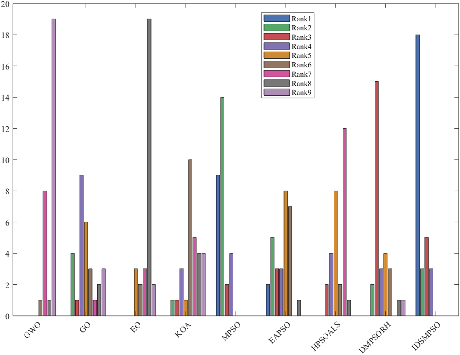
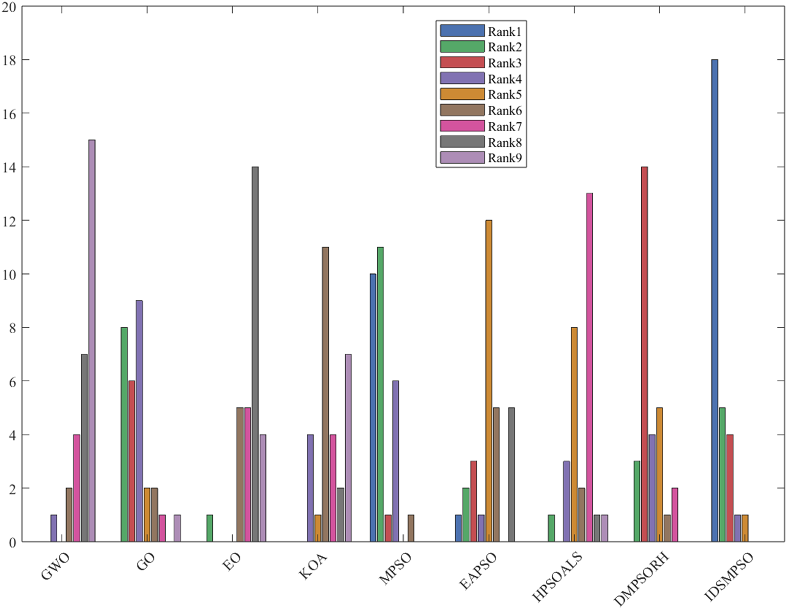
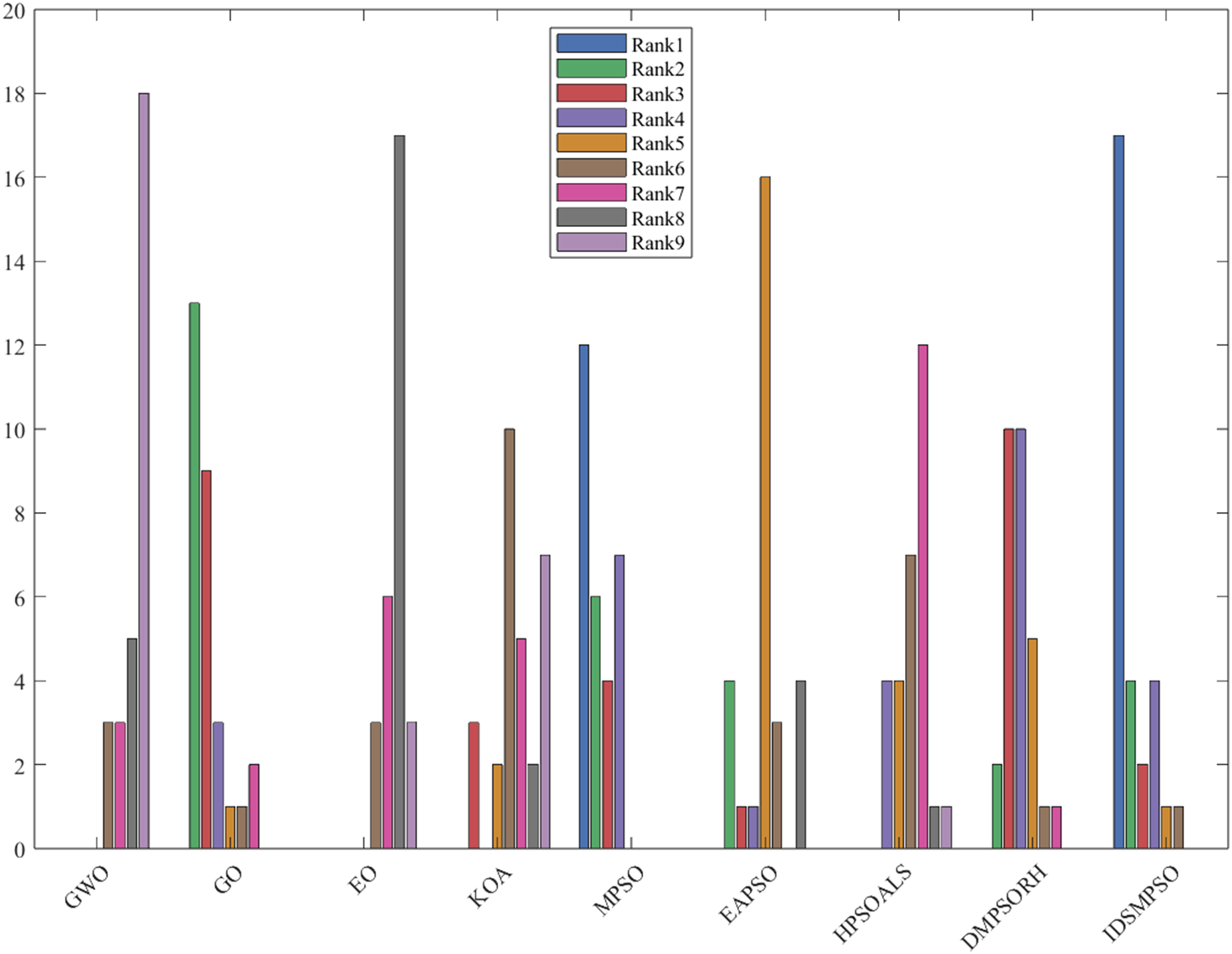
To further illustrate the superiority of IDSMPSO, Figs. 4–6 present histograms of the average value rankings for 30-, 50- and 100-dimensional problems, respectively. These histograms are primarily used to display the number of times each peer algorithm achieves rankings from 1st to 9th place. As shown in Fig. 4, under the 30-dimensional scenario, the number of times IDSMPSO secures the 1st place is nearly twice that of MPSO. Similarly, in the 50-dimensional scenario depicted in Fig. 5, our proposal also ranks as the top-performing algorithm, which significantly surpasses MPSO (ranks 2nd) and EAPSO (ranks 3rd). Furthermore, it is worth noting that in the 100-dimensional scenario shown in Fig. 6, IDSMPSO wins the 1st place slightly more times than MPSO. However, MPSO achieves the 2nd place far more frequently than IDSMPSO. This fully verifies the effectiveness of IDSMPSO in the task of numerical function optimization, at least on CEC’17 test suite.
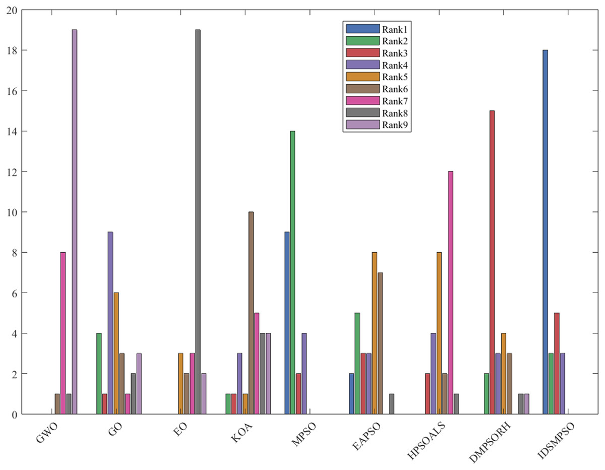
Figure 4: Rank histogram of IDSMPSO and peer algorithms (D = 30).
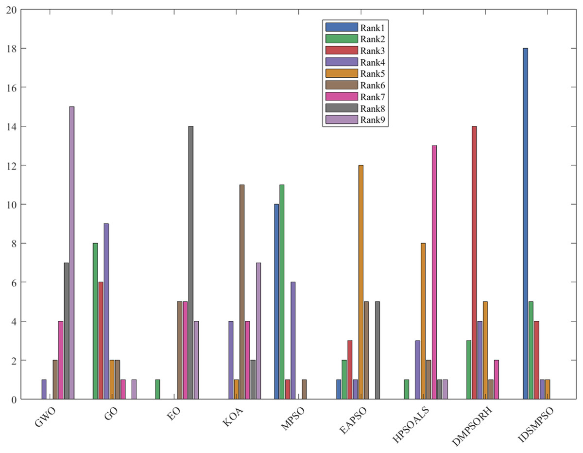
Figure 5: Rank histogram of IDSMPSO and peer algorithms (D = 50).
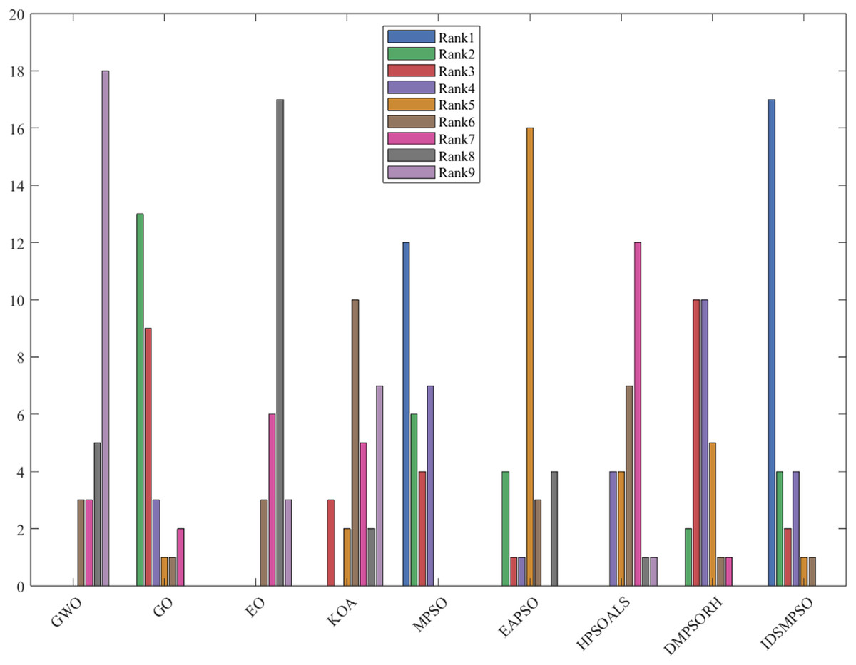
Figure 6: Rank histogram of IDSMPSO and peer algorithms (D = 100).
Convergence analysis
To analyze the convergence speed and accuracy of the proposed IDSMPSO and the comparison algorithms, we recorded and stored the best fitness value at each iteration and plotted the corresponding convergence curves. Due to the limited space, only eight representative functions are selected for testing under D = 30, 50 and 100, including two unimodal functions (f1, f3), one multimodal function (f4), two hybrid functions (f12, f13) and composition functions (f25).
As shown in Figs. 7–9, compared with other algorithms, IDSMPSO exhibits significantly faster convergence on most functions and is able to converge to the optimal value without being trapped in local optima. Taking Fig. 7B as an example, the convergence curves of these algorithms display almost the same rate of decline during the initial 50 iterations. However, IDSMPSO maintains a faster convergence speed consistently and continues to decrease compared with its peer algorithms after this stage. It is worth noting that for f12, MPSO converges toward the global optimal solution at the fastest speed, but eventually gets trapped in the local optimal value after a stable iteration phase. In contrast, although IDSMPSO takes 400 iterations to reach the optimal value, its curve basically stabilizes afterward, this indicates that IDSMPSO possesses stable local convergence capability at the end of iterations. Figure 8 presents the convergence curves of various algorithms under the 50-dimensional setting. Taking function f25 in Fig. 8 as an example, all algorithms except KOA and GWO exhibit a fast evolutionary speed during the initial 150 iterations. After this stage, KOA shows fluctuations with poor stability. Notably, the convergence curves of GWO, HPSOALS and EO do not exhibit a significant decline afterward. In comparison, the iteration curves of other algorithms tend to stabilize after 400 iterations and converge to relatively small values. Taking functions f4 and f13 in Fig. 9 as examples, it is obvious that IDSMPSO converges to a smaller value. In contrast, although IDSMPSO converges slightly slower on composite functions, it outperforms the other eight algorithms by escaping from local optima and finding more promising accuracy. The results indicate that different inertia weights for particles in IDSMPSO indeed play an important role in accelerating the searching process. However, its effectiveness is only slightly demonstrated in multimodal functions.
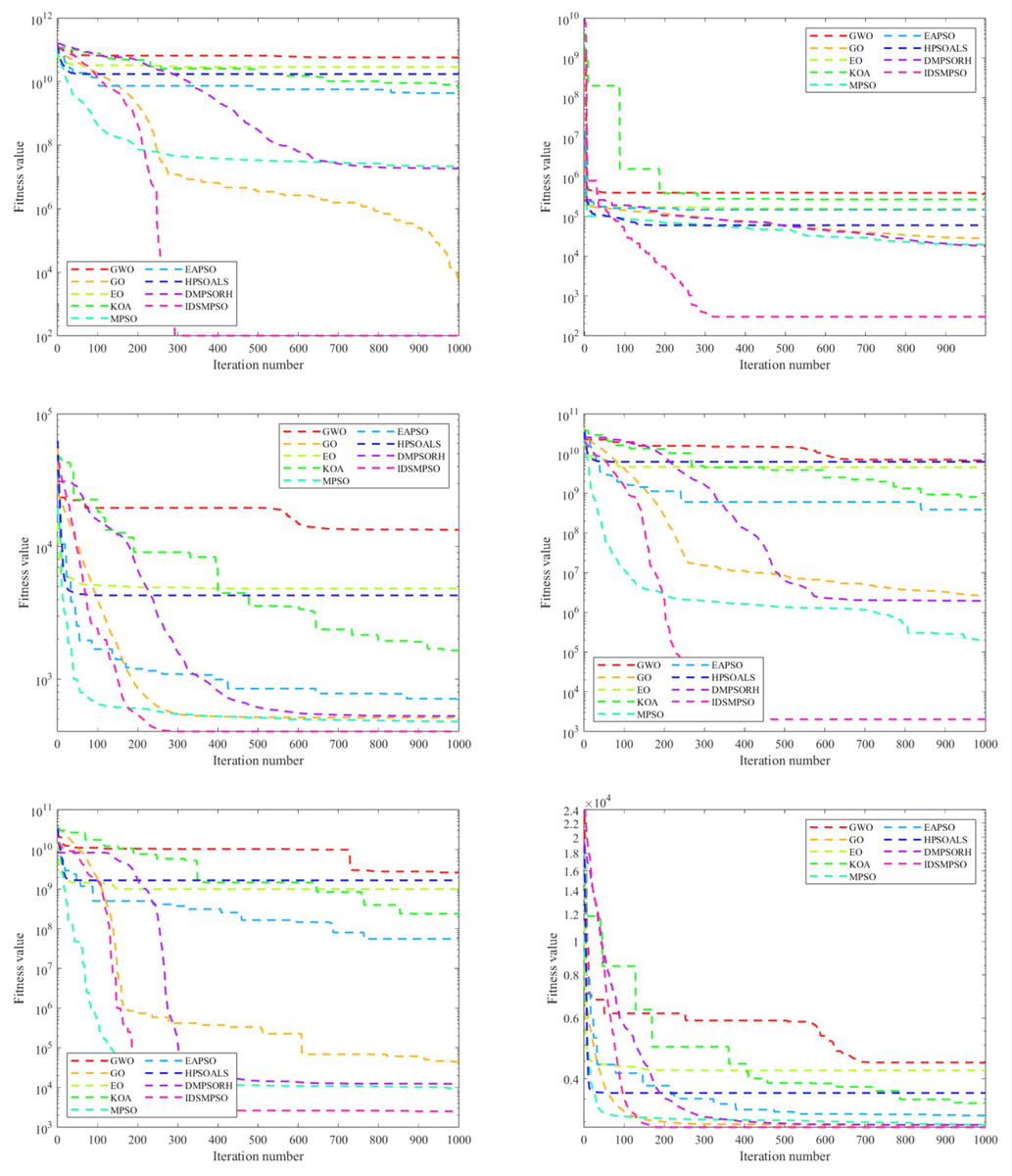
Figure 7: Convergence curves of IDSMPSO and peer algorithms (D = 30).
From left to right and top to bottom, they represent the convergence curve of function f1, f3, f4, f12, f13, f25 on the CEC’17 benchmark, respectively.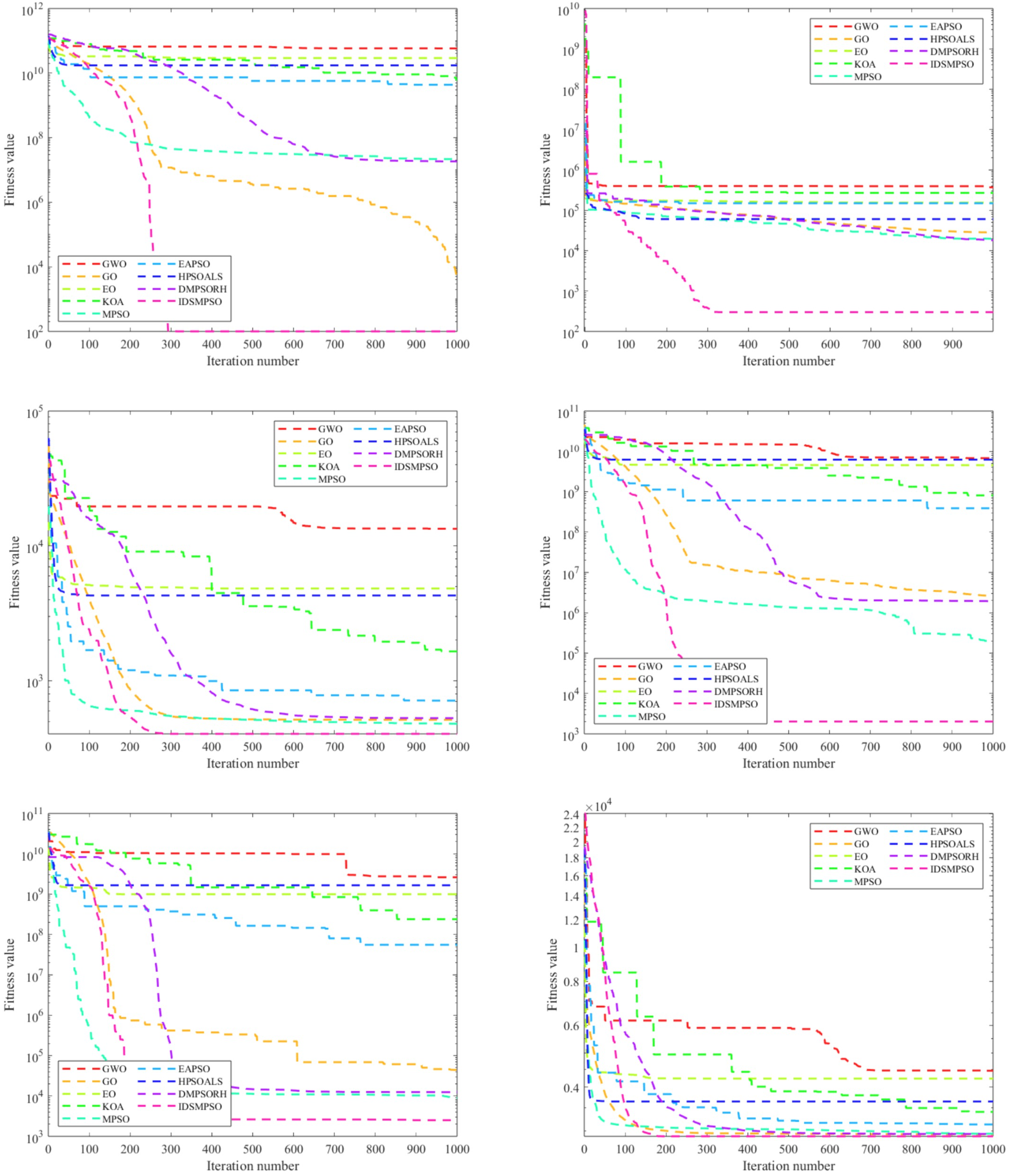
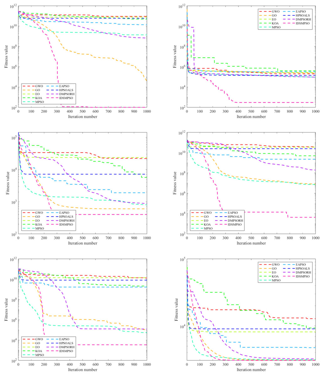
Figure 8: Convergence curves of IDSMPSO and peer algorithms (D = 50).
From left to right and top to bottom, they represent the convergence curve of function f1, f3, f4, f12, f13, f25 on the CEC’17 benchmark, respectively.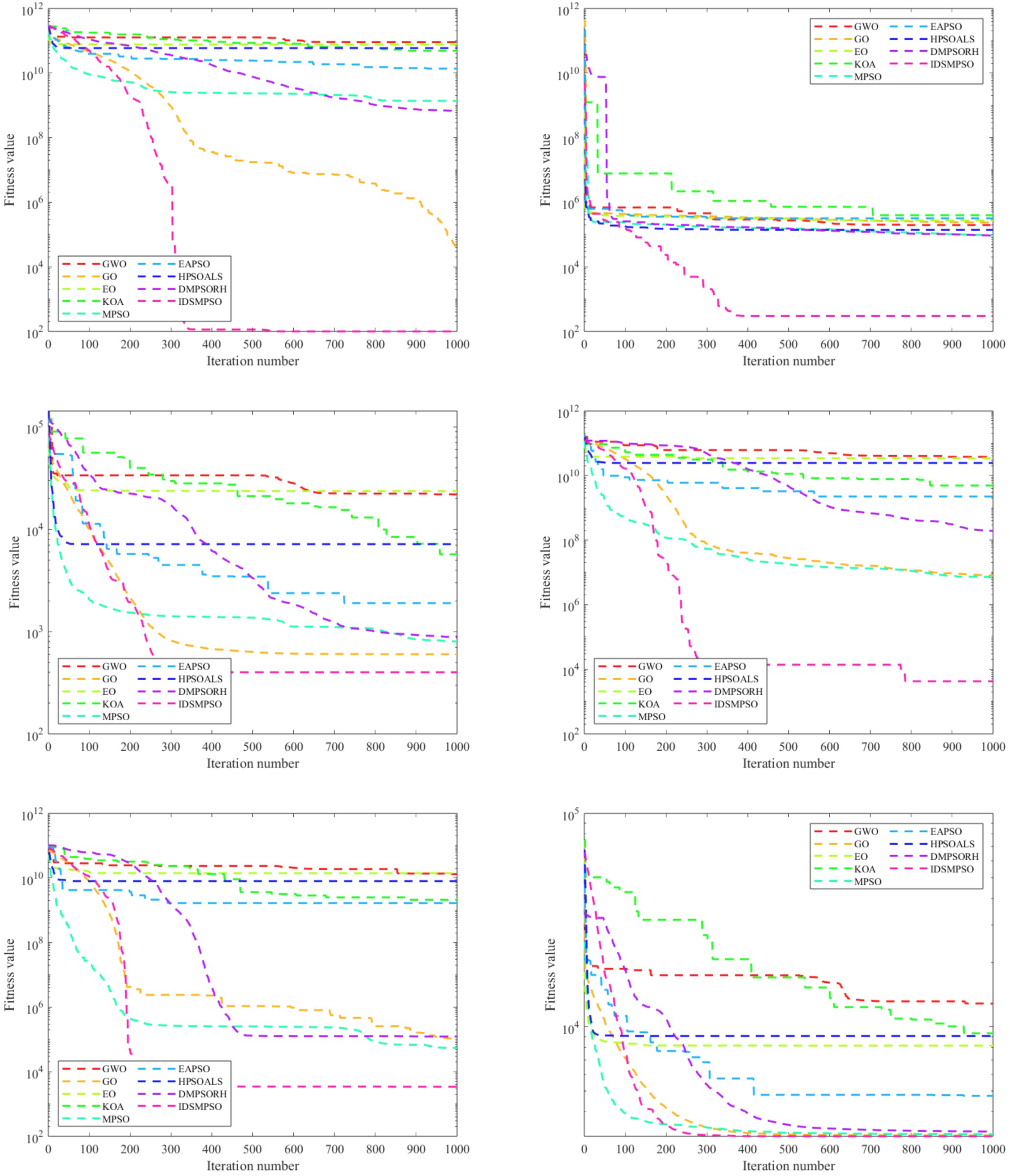
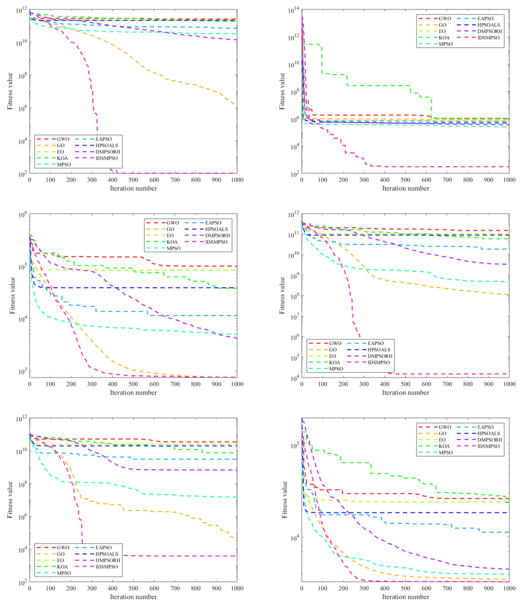
Figure 9: Convergence curves of IDSMPSO and peer algorithms (D = 100).
From left to right and top to bottom, they represent the convergence curve of function f1, f3, f4, f12, f13, f25 on the CEC’17 benchmark, respectively.
Non-parametric statistical tests
To further verify the significance of the experimental results, we employ the non-parametric Wilcoxon rank sum test in this section. The Wilcoxon rank sum test is used to compare whether there is a difference in the medians of two independent samples. The p-value (pv) determines the significance of the test, while the h-value (hv) represents the result of the hypothesis test. If the h-value is 0, the null hypothesis is accepted, indicating that there is no significant difference in the medians of the two groups. Conversely, if the h-value is 1, it indicates a significant difference, and the means are further compared. Tables 7–9 show the comparison results of four meta-heuristic algorithms and four variants of PSO in 30D, 50D and 100D, respectively, under the assumption of a significance level of 0.05. A ★ symbol indicates a significant difference between the two groups, where IDSMPSO is clearly superior to the other variants based on the mean. A ▲ symbol indicates no significant difference between the two groups, suggesting that IDSMPSO performs similarly to the other variant. A ● symbol indicates a significant difference, where IDSMPSO performs worse than the other algorithms based on the mean values.
| Func | Metric | GWO | GO | EO | KOA | MPSO | EAPSO | HPSOALS | DMPSORH |
|---|---|---|---|---|---|---|---|---|---|
| f1 | pv | 0.000★ | 0.000★ | 0.000★ | 0.000★ | 0.000★ | 0.000★ | 0.000★ | 0.000★ |
| hv | 1 | 1 | 1 | 1 | 1 | 1 | 1 | 1 | |
| f3 | pv | 0.000★ | 0.000★ | 0.000★ | 0.000★ | 0.000★ | 0.000★ | 0.000★ | 0.000★ |
| hv | 1 | 1 | 1 | 1 | 1 | 1 | 1 | 1 | |
| f4 | pv | 0.000★ | 0.000★ | 0.000★ | 0.000★ | 0.000★ | 0.000★ | 0.000★ | 0.000★ |
| hv | 1 | 1 | 1 | 1 | 1 | 1 | 1 | 1 | |
| f5 | pv | 0.000★ | 0.000★ | 0.000★ | 0.000★ | 0.000● | 0.000★ | 0.000★ | 0.145▲ |
| hv | 1 | 1 | 1 | 1 | 1 | 1 | 1 | 0 | |
| f6 | pv | 0.000★ | 0.000★ | 0.000★ | 0.000★ | 0.000● | 0.012● | 0.678▲ | 0.000★ |
| hv | 1 | 1 | 1 | 1 | 1 | 1 | 0 | 1 | |
| f7 | pv | 0.000★ | 0.000★ | 0.000★ | 0.000★ | 0.000● | 0.034● | 0.046● | 0.612▲ |
| hv | 1 | 1 | 1 | 1 | 1 | 1 | 1 | 0 | |
| f8 | pv | 0.000★ | 0.000★ | 0.000★ | 0.000★ | 0.000● | 0.000★ | 0.031★ | 0.0216● |
| hv | 1 | 1 | 1 | 1 | 1 | 1 | 1 | 1 | |
| f9 | pv | 0.000★ | 0.000★ | 0.000★ | 0.000★ | 0.000● | 0.000★ | 0.000★ | 0.000★ |
| hv | 1 | 1 | 1 | 1 | 1 | 1 | 1 | 1 | |
| f10 | pv | 0.000★ | 0.000★ | 0.000★ | 0.000★ | 0.014★ | 0.000★ | 0.000★ | 0.000★ |
| hv | 1 | 1 | 1 | 1 | 1 | 1 | 1 | 1 | |
| f11 | pv | 0.000★ | 0.000★ | 0.000★ | 0.000★ | 0.000★ | 0.000★ | 0.000★ | 0.000★ |
| hv | 1 | 1 | 1 | 1 | 1 | 1 | 1 | 1 | |
| f12 | pv | 0.000★ | 0.005★ | 0.000★ | 0.000★ | 0.010★ | 0.000★ | 0.000★ | 0.000★ |
| hv | 1 | 1 | 1 | 1 | 1 | 1 | 1 | 1 | |
| f13 | pv | 0.000★ | 0.000★ | 0.000★ | 0.000★ | 0.000★ | 0.000★ | 0.000★ | 0.000★ |
| hv | 1 | 1 | 1 | 1 | 1 | 1 | 1 | 1 | |
| f14 | pv | 0.000★ | 0.000★ | 0.000★ | 0.000★ | 0.970▲ | 0.000★ | 0.000★ | 0.000★ |
| hv | 1 | 1 | 1 | 1 | 0 | 1 | 1 | 1 | |
| f15 | pv | 0.000★ | 0.000★ | 0.000★ | 0.000★ | 0.000★ | 0.000★ | 0.000★ | 0.000★ |
| hv | 1 | 1 | 1 | 1 | 1 | 1 | 1 | 1 | |
| f16 | pv | 0.000★ | 0.000★ | 0.000★ | 0.000★ | 0.000● | 0.000★ | 0.000★ | 0.023★ |
| hv | 1 | 1 | 1 | 1 | 1 | 1 | 1 | 1 | |
| f17 | pv | 0.000★ | 0.000★ | 0.000★ | 0.000★ | 0.876▲ | 0.000★ | 0.000★ | 0.000★ |
| hv | 1 | 1 | 1 | 1 | 0 | 1 | 1 | 1 | |
| f18 | pv | 0.000★ | 0.000★ | 0.000★ | 0.000★ | 0.000★ | 0.000★ | 0.000★ | 0.000★ |
| hv | 1 | 1 | 1 | 1 | 1 | 1 | 1 | 1 | |
| f19 | pv | 0.000★ | 0.000★ | 0.000★ | 0.000★ | 0.000★ | 0.000★ | 0.000★ | 0.000★ |
| hv | 1 | 1 | 1 | 1 | 1 | 1 | 1 | 1 | |
| f20 | pv | 0.001★ | 0.000★ | 0.000★ | 0.000★ | 0.724▲ | 0.000★ | 0.000★ | 0.000★ |
| hv | 1 | 1 | 1 | 1 | 0 | 1 | 1 | 1 | |
| f21 | pv | 0.000★ | 0.000★ | 0.001★ | 0.001★ | 0.000● | 0.987▲ | 0.000★ | 0.599▲ |
| hv | 1 | 1 | 1 | 1 | 1 | 0 | 1 | 0 | |
| f22 | pv | 0.000★ | 0.000★ | 0.000★ | 0.000★ | 0.000● | 0.000● | 0.000★ | 0.000★ |
| hv | 1 | 1 | 1 | 1 | 1 | 1 | 1 | 1 | |
| f23 | pv | 0.000★ | 0.000★ | 0.000★ | 0.000★ | 0.019★ | 0.000★ | 0.000★ | 0.000★ |
| hv | 1 | 1 | 1 | 1 | 1 | 1 | 1 | 1 | |
| f24 | pv | 0.105▲ | 0.000★ | 0.363▲ | 0.000● | 0.000● | 0.000● | 0.000★ | 0.000★ |
| hv | 0 | 1 | 0 | 1 | 1 | 1 | 1 | 1 | |
| f25 | pv | 0.000★ | 0.000★ | 0.000★ | 0.000★ | 0.015★ | 0.000★ | 0.000★ | 0.000★ |
| hv | 1 | 1 | 1 | 1 | 1 | 1 | 1 | 1 | |
| f26 | pv | 0.000★ | 0.000★ | 0.000★ | 0.000★ | 0.000★ | 0.432▲ | 0.000★ | 0.000★ |
| hv | 1 | 1 | 1 | 1 | 1 | 0 | 1 | 1 | |
| f27 | pv | 0.153▲ | 0.911▲ | 0.000★ | 0.000● | 0.000★ | 0.000● | 0.046★ | 0.000★ |
| hv | 0 | 0 | 1 | 1 | 1 | 1 | 1 | 1 | |
| f28 | pv | 0.000★ | 0.000★ | 0.000★ | 0.000★ | 0.037★ | 0.000★ | 0.000★ | 0.000★ |
| hv | 1 | 1 | 1 | 1 | 1 | 1 | 1 | 1 | |
| f29 | pv | 0.000★ | 0.001★ | 0.000★ | 0.000★ | 0.613▲ | 0.000★ | 0.000★ | 0.000★ |
| hv | 1 | 1 | 1 | 1 | 0 | 1 | 1 | 1 | |
| f30 | pv | 0.000★ | 0.000★ | 0.000★ | 0.000★ | 0.000★ | 0.000★ | 0.000★ | 0.000★ |
| hv | 1 | 1 | 1 | 1 | 1 | 1 | 1 | 1 | |
| Better (★) | 27 | 28 | 28 | 27 | 16 | 22 | 27 | 25 | |
| Same (▲) | 2 | 1 | 1 | 0 | 4 | 2 | 1 | 3 | |
| Worse (●) | 0 | 0 | 0 | 2 | 9 | 5 | 1 | 1 | |
| Func | Metric | GWO | GO | EO | KOA | MPSO | EAPSO | HPSOALS | DMPSORH |
|---|---|---|---|---|---|---|---|---|---|
| f1 | pv | 0.000★ | 0.000★ | 0.000★ | 0.000★ | 0.000★ | 0.000★ | 0.000★ | 0.000★ |
| hv | 1 | 1 | 1 | 1 | 1 | 1 | 1 | 1 | |
| f3 | pv | 0.000★ | 0.000★ | 0.000★ | 0.000★ | 0.000★ | 0.000★ | 0.000★ | 0.000★ |
| hv | 1 | 1 | 1 | 1 | 1 | 1 | 1 | 1 | |
| f4 | pv | 0.000★ | 0.000★ | 0.000★ | 0.000★ | 0.000★ | 0.000★ | 0.000★ | 0.000★ |
| hv | 1 | 1 | 1 | 1 | 1 | 1 | 1 | 1 | |
| f5 | pv | 0.000★ | 0.000● | 0.000★ | 0.000★ | 0.000● | 0.000★ | 0.000● | 0.000● |
| hv | 1 | 1 | 1 | 1 | 1 | 1 | 1 | 1 | |
| f6 | pv | 0.000★ | 0.041★ | 0.000★ | 0.000★ | 0.000● | 0.000● | 0.000★ | 0.000● |
| hv | 1 | 1 | 1 | 1 | 1 | 1 | 1 | 1 | |
| f7 | pv | 0.000★ | 0.000★ | 0.000★ | 0.000★ | 0.000● | 0.006● | 0.000★ | 0.713▲ |
| hv | 1 | 1 | 1 | 1 | 1 | 1 | 1 | 0 | |
| f8 | pv | 0.000★ | 0.000★ | 0.000★ | 0.000★ | 0.000★ | 0.000★ | 0.000★ | 0.000★ |
| hv | 1 | 1 | 1 | 1 | 1 | 1 | 1 | 1 | |
| f9 | pv | 0.000★ | 0.000● | 0.000★ | 0.000★ | 0.000● | 0.003★ | 0.000★ | 0.000★ |
| hv | 1 | 1 | 1 | 1 | 1 | 1 | 1 | 1 | |
| f10 | pv | 0.000★ | 0.000★ | 0.000★ | 0.000★ | 0.013★ | 0.000★ | 0.000★ | 0.000★ |
| hv | 1 | 1 | 1 | 1 | 1 | 1 | 1 | 1 | |
| f11 | pv | 0.000★ | 0.000★ | 0.000★ | 0.000★ | 0.529▲ | 0.000★ | 0.000★ | 0.000★ |
| hv | 1 | 1 | 1 | 1 | 0 | 1 | 1 | 1 | |
| f12 | pv | 0.000★ | 0.000★ | 0.000★ | 0.000★ | 0.000★ | 0.000★ | 0.000★ | 0.000★ |
| hv | 1 | 1 | 1 | 1 | 1 | 1 | 1 | 1 | |
| f13 | pv | 0.000★ | 0.046★ | 0.000★ | 0.000★ | 0.000★ | 0.000★ | 0.000★ | 0.000★ |
| hv | 1 | 1 | 1 | 1 | 1 | 1 | 1 | 1 | |
| f14 | pv | 0.000★ | 0.025★ | 0.000★ | 0.000★ | 0.000★ | 0.000★ | 0.000★ | 0.000★ |
| hv | 1 | 1 | 1 | 1 | 1 | 1 | 1 | 1 | |
| f15 | pv | 0.000★ | 0.025★ | 0.000★ | 0.000★ | 0.415★ | 0.000★ | 0.000★ | 0.000★ |
| hv | 1 | 1 | 1 | 1 | 1 | 1 | 1 | 1 | |
| f16 | pv | 0.000★ | 0.000★ | 0.000★ | 0.000★ | 0.000● | 0.000★ | 0.000★ | 0.615▲ |
| hv | 1 | 1 | 1 | 1 | 1 | 1 | 1 | 0 | |
| f17 | pv | 0.000★ | 0.081▲ | 0.000★ | 0.000★ | 0.000● | 0.000★ | 0.000★ | 0.000★ |
| hv | 1 | 0 | 1 | 1 | 1 | 1 | 1 | 1 | |
| f18 | pv | 0.000★ | 0.000★ | 0.000★ | 0.000★ | 0.000★ | 0.000★ | 0.000★ | 0.000★ |
| hv | 1 | 1 | 1 | 1 | 1 | 1 | 1 | 1 | |
| f19 | pv | 0.000★ | 0.000★ | 0.000★ | 0.000★ | 0.005★ | 0.000★ | 0.000★ | 0.000★ |
| hv | 1 | 1 | 1 | 1 | 1 | 1 | 1 | 1 | |
| f20 | pv | 0.355▲ | 0.031★ | 0.652▲ | 0.000★ | 0.000● | 0.009★ | 0.000● | 0.017★ |
| hv | 0 | 1 | 0 | 1 | 1 | 1 | 1 | 1 | |
| f21 | pv | 0.000★ | 0.000★ | 0.000★ | 0.000★ | 0.000★ | 0.122▲ | 0.000★ | 0.000★ |
| hv | 1 | 1 | 1 | 1 | 1 | 0 | 1 | 1 | |
| f22 | pv | 0.000★ | 0.000★ | 0.000★ | 0.000★ | 0.000● | 0.000★ | 0.000★ | 0.000★ |
| hv | 1 | 1 | 1 | 1 | 1 | 1 | 1 | 1 | |
| f23 | pv | 0.000★ | 0.000★ | 0.000★ | 0.000★ | 0.015★ | 0.000★ | 0.000★ | 0.000★ |
| hv | 1 | 1 | 1 | 1 | 1 | 1 | 1 | 1 | |
| f24 | pv | 0.000★ | 0.000★ | 0.000★ | 0.000★ | 0.156▲ | 0.000★ | 0.000★ | 0.000★ |
| hv | 1 | 1 | 1 | 1 | 0 | 1 | 1 | 1 | |
| f25 | pv | 0.000★ | 0.000★ | 0.000★ | 0.000★ | 0.000★ | 0.000★ | 0.000★ | 0.000★ |
| hv | 1 | 1 | 1 | 1 | 1 | 1 | 1 | 1 | |
| f26 | pv | 0.000★ | 0.000★ | 0.000★ | 0.065▲ | 0.000● | 0.000● | 0.000★ | 0.652▲ |
| hv | 1 | 1 | 1 | 0 | 1 | 1 | 1 | 0 | |
| f27 | pv | 0.000★ | 0.000★ | 0.000★ | 0.000★ | 0.021★ | 0.000★ | 0.000★ | 0.000★ |
| hv | 1 | 1 | 1 | 1 | 1 | 1 | 1 | 1 | |
| f28 | pv | 0.000★ | 0.000★ | 0.000★ | 0.000★ | 0.000★ | 0.000★ | 0.000★ | 0.000★ |
| hv | 1 | 1 | 1 | 1 | 1 | 1 | 1 | 1 | |
| f29 | pv | 0.000★ | 0.000★ | 0.000★ | 0.000★ | 0.313★ | 0.000★ | 0.000★ | 0.000★ |
| hv | 1 | 1 | 1 | 1 | 1 | 1 | 1 | 1 | |
| f30 | pv | 0.000★ | 0.013★ | 0.000★ | 0.000★ | 0.000● | 0.000★ | 0.000★ | 0.000★ |
| hv | 1 | 1 | 1 | 1 | 1 | 1 | 1 | 1 | |
| Better (★) | 28 | 26 | 28 | 28 | 17 | 25 | 27 | 24 | |
| Same (▲) | 1 | 1 | 1 | 1 | 2 | 1 | 0 | 3 | |
| Worse (●) | 0 | 2 | 0 | 0 | 10 | 3 | 2 | 2 | |
| Func | Metric | GWO | GO | EO | KOA | MPSO | EAPSO | HPSOALS | DMPSORH |
|---|---|---|---|---|---|---|---|---|---|
| f1 | pv | 0.000★ | 0.000★ | 0.000★ | 0.000★ | 0.000★ | 0.000★ | 0.000★ | 0.000★ |
| hv | 1 | 1 | 1 | 1 | 1 | 1 | 1 | 1 | |
| f3 | pv | 0.000★ | 0.000★ | 0.000★ | 0.000★ | 0.000★ | 0.000★ | 0.000★ | 0.000★ |
| hv | 1 | 1 | 1 | 1 | 1 | 1 | 1 | 1 | |
| f4 | pv | 0.000★ | 0.000★ | 0.000★ | 0.000★ | 0.000★ | 0.000★ | 0.000★ | 0.000★ |
| hv | 1 | 1 | 1 | 1 | 1 | 1 | 1 | 1 | |
| f5 | pv | 0.000★ | 0.090▲ | 0.000★ | 0.000★ | 0.000● | 0.000★ | 0.000★ | 0.000● |
| hv | 1 | 0 | 1 | 1 | 1 | 1 | 1 | 1 | |
| f6 | pv | 0.000★ | 0.041● | 0.000★ | 0.000★ | 0.117▲ | 0.526▲ | 0.000★ | 0.000● |
| hv | 1 | 1 | 1 | 1 | 0 | 0 | 1 | 1 | |
| f7 | pv | 0.000★ | 0.000● | 0.000★ | 0.000★ | 0.000● | 0.021★ | 0.000★ | 0.000★ |
| hv | 1 | 1 | 1 | 1 | 1 | 1 | 1 | 1 | |
| f8 | pv | 0.000★ | 0.000★ | 0.000★ | 0.000★ | 0.000★ | 0.000★ | 0.000★ | 0.000★ |
| hv | 1 | 1 | 1 | 1 | 1 | 1 | 1 | 1 | |
| f9 | pv | 0.000★ | 0.000● | 0.000★ | 0.000★ | 0.000● | 0.003★ | 0.000★ | 0.040★ |
| hv | 1 | 1 | 1 | 1 | 1 | 1 | 1 | 1 | |
| f10 | pv | 0.630▲ | 0.000★ | 0.695▲ | 0.000★ | 0.000★ | 0.096▲ | 0.000★ | 0.000★ |
| hv | 0 | 1 | 0 | 1 | 1 | 0 | 1 | 1 | |
| f11 | pv | 0.000★ | 0.000★ | 0.000★ | 0.000★ | 0.009★ | 0.000★ | 0.000★ | 0.000★ |
| hv | 1 | 1 | 1 | 1 | 1 | 1 | 1 | 1 | |
| f12 | pv | 0.000★ | 0.000★ | 0.000★ | 0.000★ | 0.000★ | 0.000★ | 0.000★ | 0.000★ |
| hv | 1 | 1 | 1 | 1 | 1 | 1 | 1 | 1 | |
| f13 | pv | 0.000★ | 0.046★ | 0.000★ | 0.000★ | 0.000★ | 0.000★ | 0.000★ | 0.000★ |
| hv | 1 | 1 | 1 | 1 | 1 | 1 | 1 | 1 | |
| f14 | pv | 0.000★ | 0.739▲ | 0.000★ | 0.000★ | 0.001★ | 0.000★ | 0.000★ | 0.000★ |
| hv | 1 | 0 | 1 | 1 | 1 | 1 | 1 | 1 | |
| f15 | pv | 0.000★ | 0.025★ | 0.000★ | 0.000★ | 0.415★ | 0.000★ | 0.000★ | 0.000★ |
| hv | 1 | 1 | 1 | 1 | 1 | 1 | 1 | 1 | |
| f16 | pv | 0.000★ | 0.000★ | 0.000★ | 0.000★ | 0.267▲ | 0.000★ | 0.000★ | 0.000★ |
| hv | 1 | 1 | 1 | 1 | 0 | 1 | 1 | 1 | |
| f17 | pv | 0.000★ | 0.000★ | 0.000★ | 0.000★ | 0.031★ | 0.000★ | 0.000★ | 0.000★ |
| hv | 1 | 1 | 1 | 1 | 1 | 1 | 1 | 1 | |
| f18 | pv | 0.000★ | 0.019★ | 0.000★ | 0.000★ | 0.000★ | 0.000★ | 0.000★ | 0.000★ |
| hv | 1 | 1 | 1 | 1 | 1 | 1 | 1 | 1 | |
| f19 | pv | 0.000★ | 0.589▲ | 0.000★ | 0.000★ | 0.005★ | 0.000★ | 0.000★ | 0.000★ |
| hv | 1 | 0 | 1 | 1 | 1 | 1 | 1 | 1 | |
| f20 | pv | 0.016★ | 0.000★ | 0.035★ | 0.000★ | 0.000● | 0.000★ | 0.003★ | 0.000★ |
| hv | 1 | 1 | 1 | 1 | 1 | 1 | 1 | 1 | |
| f21 | pv | 0.000★ | 0.000★ | 0.000★ | 0.000● | 0.081▲ | 0.000● | 0.082▲ | 0.429▲ |
| hv | 1 | 1 | 1 | 1 | 0 | 1 | 0 | 0 | |
| f22 | pv | 0.000★ | 0.000★ | 0.000★ | 0.000★ | 0.825▲ | 0.000★ | 0.000★ | 0.000★ |
| hv | 1 | 1 | 1 | 1 | 0 | 1 | 1 | 1 | |
| f23 | pv | 0.304▲ | 0.004★ | 0.620▲ | 0.000★ | 0.000● | 0.000● | 0.000★ | 0.008★ |
| hv | 0 | 1 | 0 | 1 | 1 | 1 | 1 | 1 | |
| f24 | pv | 0.000★ | 0.019★ | 0.000★ | 0.000● | 0.000● | 0.000● | 0.000★ | 0.059▲ |
| hv | 1 | 1 | 1 | 1 | 1 | 1 | 1 | 0 | |
| f25 | pv | 0.000★ | 0.000★ | 0.000★ | 0.000★ | 0.000★ | 0.000★ | 0.000★ | 0.000★ |
| hv | 1 | 1 | 1 | 1 | 1 | 1 | 1 | 1 | |
| f26 | pv | 0.000★ | 0.000● | 0.000★ | 0.065▲ | 0.000● | 0.000● | 0.000● | 0.000● |
| hv | 1 | 1 | 1 | 0 | 1 | 1 | 1 | 1 | |
| f27 | pv | 0.272▲ | 0.000★ | 0.528▲ | 0.000★ | 0.000● | 0.000★ | 0.994▲ | 0.000★ |
| hv | 0 | 1 | 0 | 1 | 1 | 1 | 0 | 1 | |
| f28 | pv | 0.000★ | 0.000★ | 0.000★ | 0.000★ | 0.000★ | 0.000★ | 0.000★ | 0.000★ |
| hv | 1 | 1 | 1 | 1 | 1 | 1 | 1 | 1 | |
| f29 | pv | 0.000★ | 0.000★ | 0.000★ | 0.000★ | 0.000● | 0.000★ | 0.000★ | 0.000★ |
| hv | 1 | 1 | 1 | 1 | 1 | 1 | 1 | 1 | |
| f30 | pv | 0.000★ | 0.000★ | 0.000★ | 0.000★ | 0.000★ | 0.000★ | 0.000★ | 0.000★ |
| hv | 1 | 1 | 1 | 1 | 1 | 1 | 1 | 1 | |
| Better (★) | 26 | 22 | 26 | 26 | 16 | 23 | 26 | 24 | |
| Same (▲) | 3 | 3 | 3 | 1 | 4 | 2 | 2 | 2 | |
| Worse (●) | 0 | 4 | 0 | 2 | 9 | 4 | 1 | 3 | |
As can be observed from Table 7, IDSMPSO exhibits significant advantages over four state-of-the-art optimizers (GWO, GO, EO, KOA). Specifically, it outperforms GWO, GO, EO and KOA on 27, 28, 28 and 27 test functions, respectively. However, GWO, GO and EO achieve performance comparable to IDSMPSO on 2, 1 and 1 test functions, respectively. When compared with four classical PSO variants (MPSO, EAPSO, HPSOALS, DMPSORH), IDSMPSO retains its superiority, which surpasses these four algorithms on 16, 22, 27 and 25 functions, respectively. Additionally, IDSMPSO shows similar performance to these PSO variants on 4, 2, 1 and 3 functions, respectively. It can be seen from Table 8 that compared with the 30-dimensional scenario, IDSMPSO obtains more favorable comparison results against other peer algorithms in the 50-dimensional scenario. Specifically, it finds better solutions than GWO, GO, EO, KOA, HPSOALS and EAPSO on more than 83% of the test functions, furthermore, none of these peer algorithms outperforms IDSMPSO on any function. Among the aforementioned peer algorithms, MPSO delivers relatively strong performance. Yet, it can still only surpass IDSMPSO on 10 functions. In addition, IDSMPSO still demonstrates remarkable performance advantages in Table 9. Specifically, IDSMPSO almost completely outperforms GWO, EO, KOA and HPSOALS. It is worth noting that GO, MPSO, EAPSO and DMPSORH surpass IDSMPSO on 4, 9, 4 and 3 test functions, respectively. Obviously, in each dimension, IDSMPSO performs better than the compared algorithms on at least half of the test functions. This further verifies the excellent global search capability of IDSMPSO.
In addition, the boxplot is employed to illustrate the differences of the mean values obtained by the comparison algorithms and to analyze their stability. Figures 10–12 present the boxplots of the global minimum results of f3, f4, f11 and f28 based on 30-, 50- and 100-dimensional cases. As shown in these figures, IDSMPSO achieves a relatively narrow distribution of optimal solutions in 30D and 50D. From Fig. 12, it can be observed that the box for IDSMPSO is relatively flat. The degree of flatness generally reflects the stability of the algorithm—the flatter the box, the more stable the algorithm. Additionally, IDSMPSO achieves significant results in both minimum values and medians.
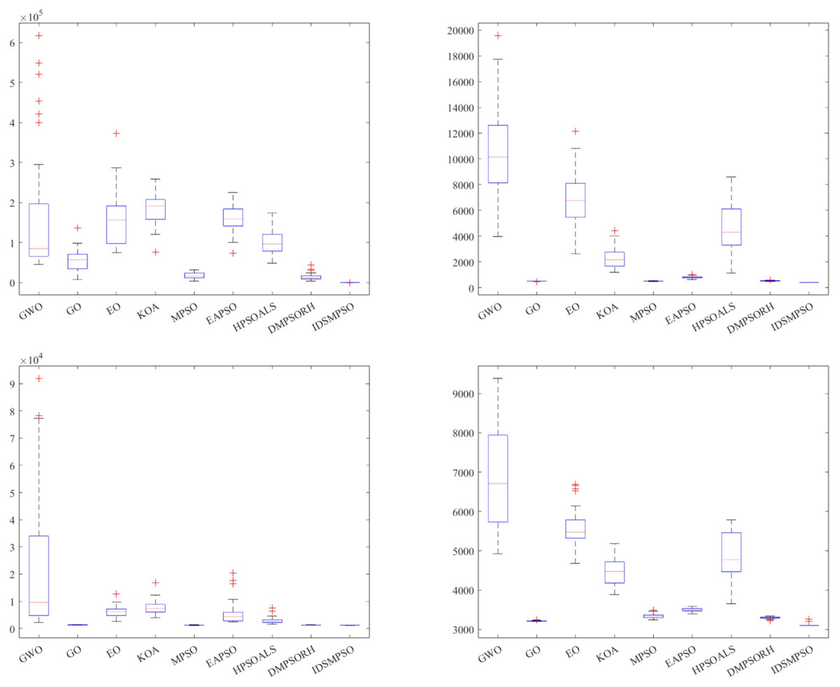
Figure 10: Boxplot for different algorithms on CEC’17 (D = 30).
From left to right and top to bottom, they represent the boxplot of function f3, f4, f11, f28 on the CEC’17 benchmark, respectively.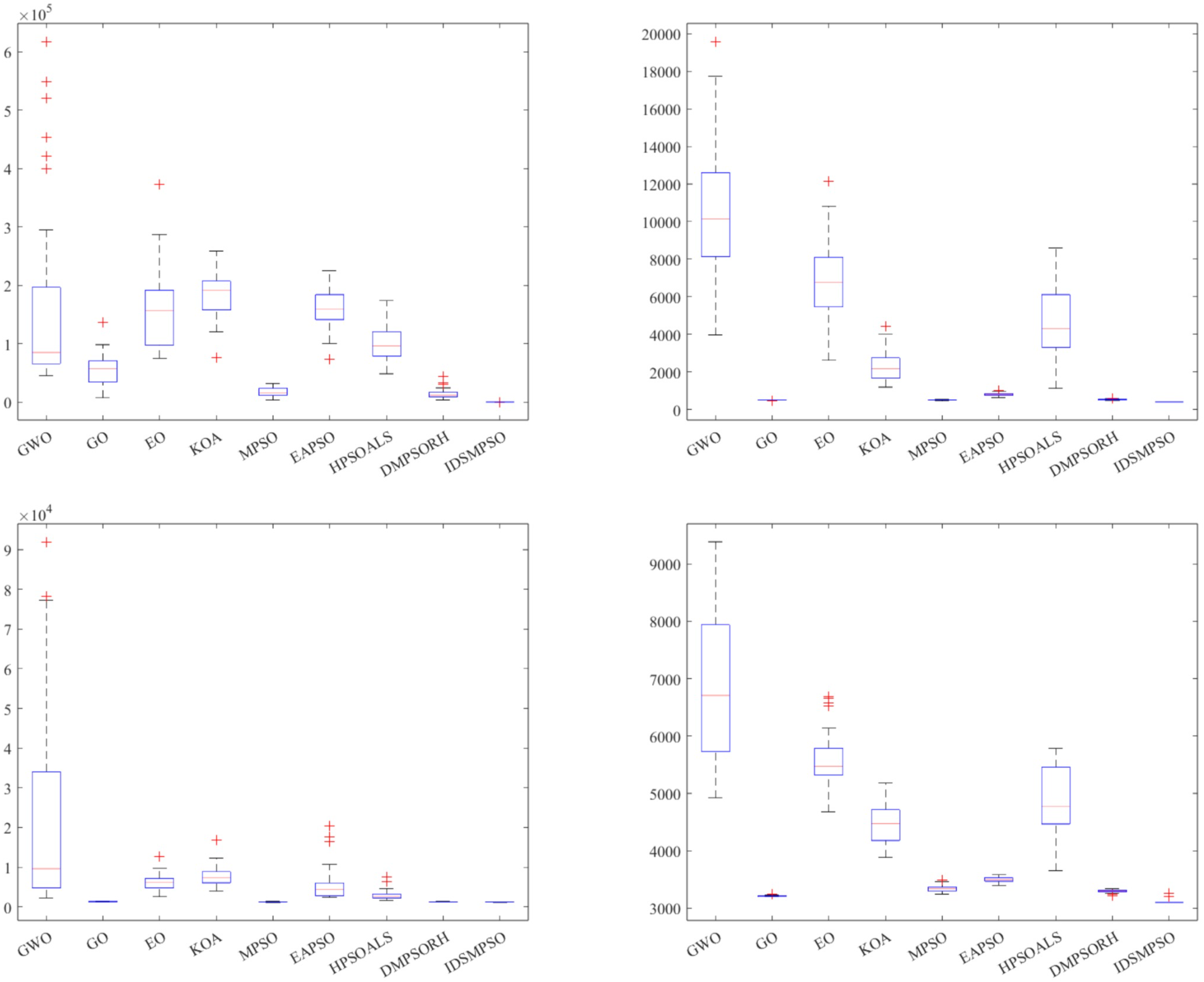
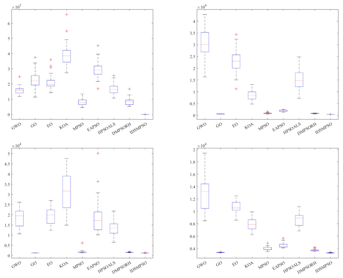
Figure 11: Boxplot for different algorithms on CEC’17 (D = 50).
From left to right and top to bottom, they represent the boxplot of function f3, f4, f11, f28 on the CEC’17 benchmark, respectively.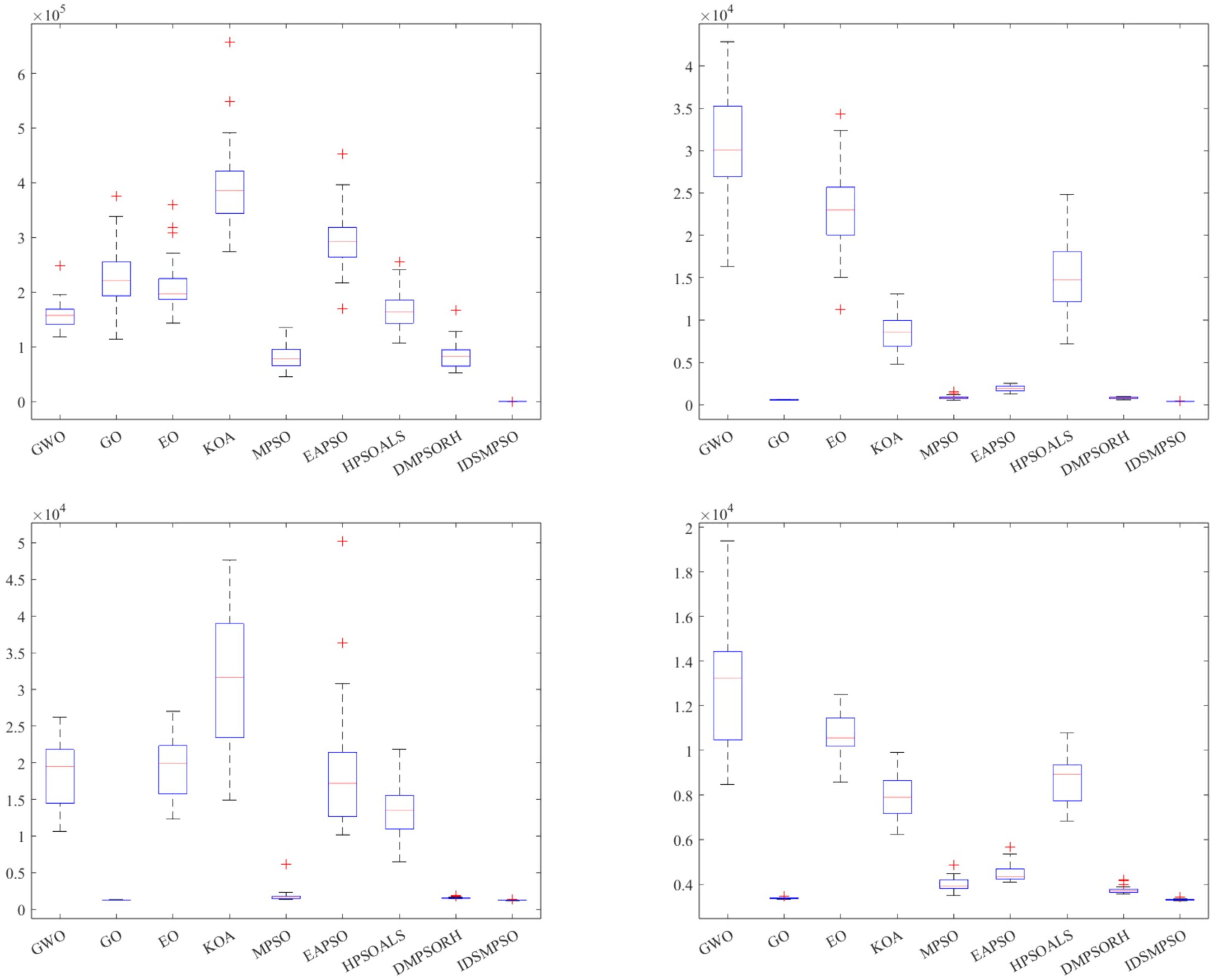
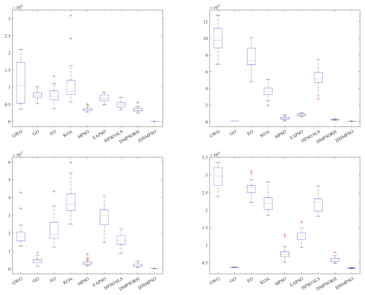
Figure 12: Boxplot for different algorithms on CEC’17 (D = 100).
From left to right and top to bottom, they represent the boxplot of function f3, f4, f11, f28 on the CEC’17 benchmark, respectively.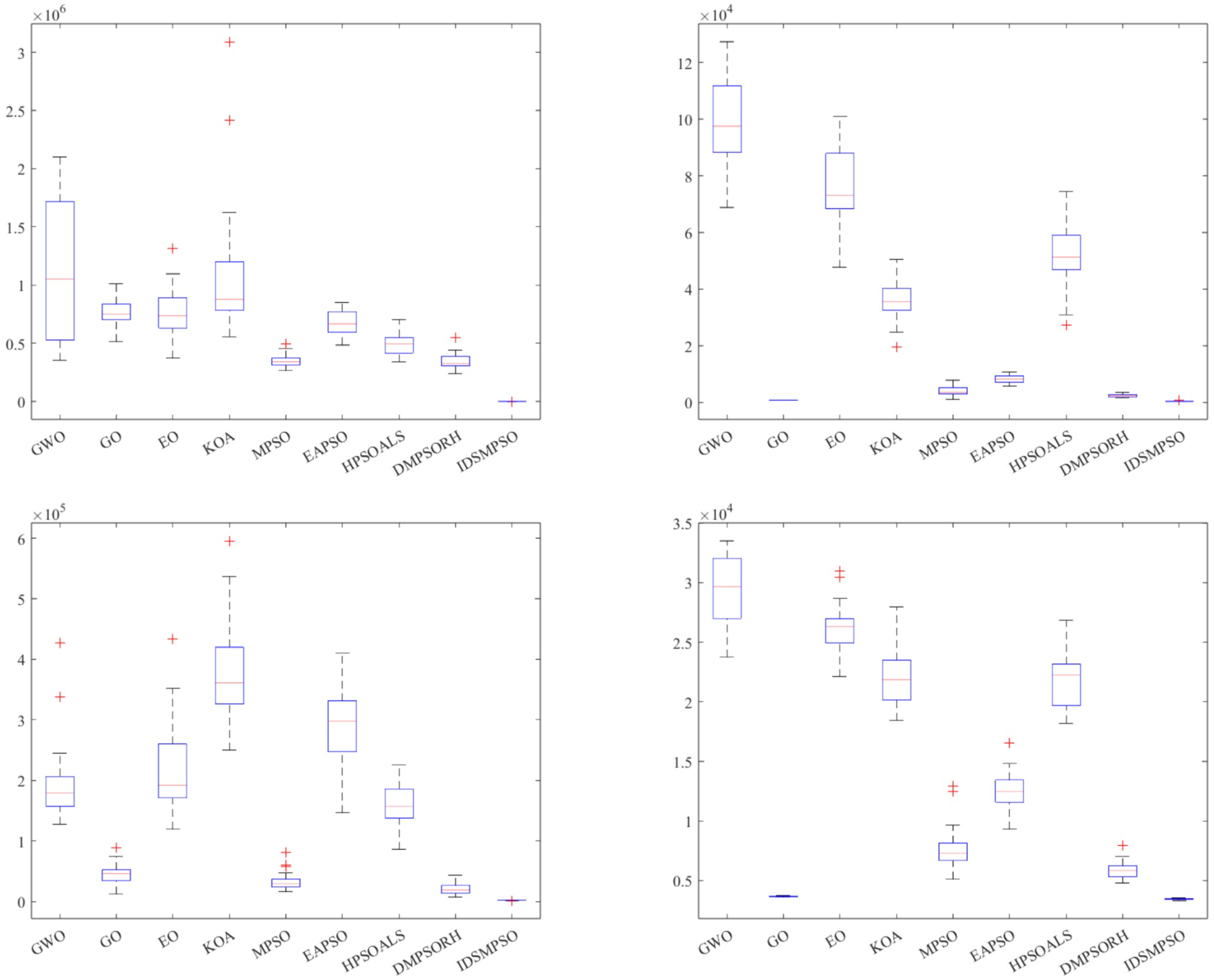
To conduct a more detailed analysis of all algorithms, the Friedman test across different dimensions is performed (D = 30, 50 and 100). Table 10 demonstrates that IDSMPSO also performs excellently under 30-dimensional conditions, followed by MPSO, DMPSORH, EAPSO, GO, HPSOALS, KOA, EO and GWO. In Table 11, it is apparent that IDSMPSO achieves the best average Friedman value in the 50-dimensional case, followed by MPSO, GO, DMPSORH, EAPSO, HPSOALS, KOA, EO and GWO. As seen in Table 12, IDSMPSO can obtain significant results based on the average Friedman values in the 100-dimensional case, followed by MPSO, GO, DMPSORH, EAPSO, HPSOALS, KOA, EO and GWO. In a nutshell, IDSMPSO exhibits excellent performance across three different dimensions on CEC’17. Meanwhile, MPSO and GO also yield better optimization results. It is worth noting that the Friedman value (f-value) of the best results is highlighted in bold in Tables 10, 11 and 12.
| Func | Metric | GWO | GO | EO | KOA | MPSO | EAPSO | HPSOALS | DMPSORH | IDSMPSO |
|---|---|---|---|---|---|---|---|---|---|---|
| f1 | f-value | 8.67 | 2.03 | 8.23 | 6.03 | 3.43 | 5.00 | 7.07 | 3.53 | 1.00 |
| f3 | f-value | 5.97 | 4.23 | 7.47 | 8.37 | 2.63 | 7.23 | 5.47 | 2.63 | 1.00 |
| f4 | f-value | 8.40 | 2.60 | 8.37 | 6.10 | 2.77 | 5.00 | 7.13 | 3.63 | 1.00 |
| f5 | f-value | 8.13 | 6.10 | 7.73 | 6.93 | 1.00 | 3.90 | 4.03 | 2.67 | 2.81 |
| f6 | f-value | 6.57 | 6.57 | 8.53 | 4.57 | 1.00 | 2.93 | 5.03 | 4.57 | 3.03 |
| f7 | f-value | 8.03 | 7.60 | 7.60 | 5.63 | 1.00 | 3.17 | 3.67 | 4.40 | 3.71 |
| f8 | f-value | 7.93 | 4.13 | 7.20 | 7.83 | 1.00 | 5.63 | 3.93 | 2.30 | 2.41 |
| f9 | f-value | 7.17 | 4.17 | 7.67 | 7.43 | 1.00 | 2.83 | 4.13 | 3.67 | 1.37 |
| f10 | f-value | 6.87 | 2.50 | 5.83 | 8.70 | 1.27 | 7.20 | 4.33 | 5.77 | 1.13 |
| f11 | f-value | 8.00 | 3.77 | 7.57 | 7.97 | 1.80 | 5.80 | 5.67 | 2.77 | 1.67 |
| f12 | f-value | 8.37 | 3.57 | 8.43 | 6.03 | 2.47 | 5.03 | 7.13 | 2.97 | 1.00 |
| f13 | f-value | 7.80 | 3.73 | 8.20 | 6.50 | 2.27 | 5.80 | 6.70 | 2.93 | 1.07 |
| f14 | f-value | 6.40 | 4.13 | 7.93 | 7.57 | 2.70 | 6.87 | 5.57 | 2.80 | 1.03 |
| f15 | f-value | 6.50 | 4.10 | 7.43 | 8.03 | 1.83 | 7.73 | 5.07 | 3.03 | 1.27 |
| f16 | f-value | 8.43 | 5.13 | 7.10 | 7.13 | 1.23 | 4.50 | 5.70 | 3.23 | 2.53 |
| f17 | f-value | 7.53 | 6.07 | 6.83 | 7.07 | 1.40 | 4.03 | 4.47 | 4.30 | 1.30 |
| f18 | f-value | 7.53 | 4.00 | 7.43 | 7.97 | 2.83 | 6.53 | 4.87 | 2.83 | 1.00 |
| f19 | f-value | 6.03 | 4.33 | 7.47 | 7.97 | 2.30 | 7.57 | 5.63 | 2.60 | 1.10 |
| f20 | f-value | 5.53 | 7.33 | 5.57 | 7.77 | 1.30 | 4.80 | 3.83 | 5.70 | 1.17 |
| f21 | f-value | 6.40 | 8.17 | 7.50 | 6.13 | 1.00 | 3.83 | 4.40 | 3.67 | 4.40 |
| f22 | f-value | 7.47 | 5.07 | 7.17 | 5.13 | 1.10 | 3.20 | 5.90 | 5.70 | 3.27 |
| f23 | f-value | 6.60 | 7.70 | 6.03 | 3.23 | 1.51 | 2.07 | 7.10 | 7.33 | 1.26 |
| f24 | f-value | 6.77 | 8.33 | 6.23 | 3.17 | 1.40 | 1.13 | 7.23 | 6.07 | 3.25 |
| f25 | f-value | 8.83 | 2.50 | 8.00 | 6.57 | 2.73 | 5.03 | 6.57 | 3.50 | 1.27 |
| f26 | f-value | 8.10 | 5.30 | 8.00 | 3.97 | 2.10 | 1.60 | 6.17 | 5.90 | 1.32 |
| f27 | f-value | 6.77 | 7.50 | 6.37 | 1.50 | 4.07 | 1.07 | 6.73 | 7.43 | 1.90 |
| f28 | f-value | 8.63 | 2.03 | 8.10 | 6.33 | 3.53 | 4.97 | 6.93 | 3.40 | 1.07 |
| f29 | f-value | 8.53 | 5.30 | 7.77 | 6.10 | 1.00 | 4.00 | 6.10 | 3..43 | 2.03 |
| f30 | f-value | 8.30 | 4.00 | 7.87 | 6.53 | 1.43 | 5.70 | 6.57 | 3.03 | 1.21 |
| AR | 7.45 | 4.89 | 7.43 | 6.35 | 1.90 | 4.62 | 5.62 | 4.01 | 1.77 | |
| FR | 9 | 5 | 8 | 7 | 2 | 4 | 6 | 3 | 1 | |
| Func | Metric | GWO | GO | EO | KOA | MPSO | EAPSO | HPSOALS | DMPSORH | IDSMPSO |
|---|---|---|---|---|---|---|---|---|---|---|
| f1 | f-value | 8.97 | 2.03 | 7.90 | 6.07 | 3.57 | 5.00 | 7.07 | 3.40 | 1.00 |
| f3 | f-value | 4.50 | 6.53 | 6.43 | 8.77 | 2.53 | 7.80 | 4.87 | 2.57 | 1.00 |
| f4 | f-value | 8.77 | 2.07 | 8.00 | 6.10 | 3.40 | 5.00 | 7.13 | 3.53 | 1.00 |
| f5 | f-value | 8.03 | 3.10 | 7.53 | 7.33 | 1.03 | 5.50 | 4.73 | 2.10 | 4.63 |
| f6 | f-value | 8.27 | 4.47 | 8.37 | 5.70 | 1.00 | 2.93 | 6.17 | 3.30 | 4.80 |
| f7 | f-value | 7.90 | 5.40 | 7.80 | 7.90 | 1.00 | 2.90 | 4.03 | 3.90 | 3.17 |
| f8 | f-value | 7.53 | 3.20 | 7.80 | 7.17 | 1.30 | 5.40 | 4.40 | 2.30 | 1.00 |
| f9 | f-value | 7.53 | 3.20 | 7.80 | 7.17 | 1.00 | 5.40 | 4.40 | 2.30 | 3.07 |
| f10 | f-value | 6.60 | 2.47 | 6.27 | 8.73 | 1.10 | 7.37 | 4.33 | 5.50 | 1.00 |
| f11 | f-value | 6.97 | 1.90 | 6.90 | 8.67 | 3.63 | 6.70 | 5.77 | 3.37 | 1.10 |
| f12 | f-value | 8.37 | 2.50 | 8.30 | 6.00 | 2.83 | 5.00 | 7.33 | 3.67 | 1.00 |
| f13 | f-value | 8.53 | 3.47 | 8.13 | 5.93 | 2.37 | 5.07 | 7.33 | 3.17 | 1.00 |
| f14 | f-value | 8.33 | 3.23 | 7.97 | 6.87 | 2.97 | 5.60 | 6.23 | 2.80 | 1.00 |
| f15 | f-value | 8.17 | 3.60 | 8.27 | 6.10 | 2.57 | 5.83 | 6.63 | 2.83 | 1.00 |
| f16 | f-value | 7.80 | 3.73 | 8.13 | 7.17 | 1.13 | 5.07 | 6.47 | 2.73 | 2.77 |
| f17 | f-value | 6.27 | 2.83 | 8.47 | 7.77 | 1.23 | 6.10 | 4.70 | 3.70 | 2.51 |
| f18 | f-value | 7.60 | 3.27 | 6.93 | 8.03 | 3.33 | 6.30 | 6.13 | 2.40 | 1.00 |
| f19 | f-value | 8.00 | 4.00 | 8.23 | 6.27 | 2.23 | 6.10 | 6.40 | 2.73 | 1.03 |
| f20 | f-value | 5.93 | 4.30 | 5.67 | 8.83 | 1.23 | 7.00 | 3.00 | 5.43 | 3.60 |
| f21 | f-value | 8.27 | 1.50 | 8.13 | 6.00 | 3.37 | 4.20 | 7.60 | 4.43 | 1.50 |
| f22 | f-value | 6.30 | 2.60 | 6.27 | 8.70 | 1.07 | 7.07 | 4.33 | 6.17 | 2.01 |
| f23 | f-value | 7.13 | 7.50 | 6.23 | 3.03 | 1.80 | 2.00 | 6.07 | 7.00 | 1.00 |
| f24 | f-value | 8.20 | 6.77 | 6.87 | 3.13 | 1.00 | 2.07 | 7.73 | 4.87 | 1.56 |
| f25 | f-value | 8.73 | 2.00 | 8.00 | 6.63 | 3.87 | 4.97 | 6.63 | 3.17 | 1.00 |
| f26 | f-value | 8.50 | 3.53 | 8.20 | 4.67 | 1.47 | 1.03 | 7.13 | 4.87 | 1.88 |
| f27 | f-value | 6.87 | 6.70 | 6.90 | 3.73 | 1.13 | 1.93 | 7.30 | 6.80 | 1.05 |
| f28 | f-value | 8.77 | 1.90 | 8.13 | 6.23 | 3.83 | 4.93 | 6.87 | 3.23 | 1.10 |
| f29 | f-value | 8.77 | 3.90 | 7.87 | 6.07 | 1.53 | 4.40 | 7.07 | 3.70 | 1.23 |
| f30 | f-value | 8.40 | 3.67 | 8.20 | 6.40 | 1.00 | 5.63 | 6.37 | 3.13 | 2.20 |
| AR | 7.72 | 3.63 | 7.57 | 6.59 | 2.05 | 4.97 | 6.00 | 3.76 | 1.80 | |
| FR | 9 | 3 | 8 | 7 | 2 | 5 | 6 | 4 | 1 | |
| Func | Metric | GWO | GO | EO | KOA | MPSO | EAPSO | HPSOALS | DMPSORH | IDSMPSO |
|---|---|---|---|---|---|---|---|---|---|---|
| f1 | f-value | 8.80 | 2.00 | 8.07 | 6.63 | 3.93 | 5.00 | 6.50 | 3.07 | 1.00 |
| f3 | f-value | 6.97 | 6.90 | 6.60 | 7.97 | 2.73 | 5.97 | 4.17 | 2.70 | 1.00 |
| f4 | f-value | 8.87 | 1.93 | 8.07 | 6.17 | 3.77 | 5.00 | 6.90 | 3.23 | 1.07 |
| f5 | f-value | 7.73 | 2.43 | 7.23 | 7.17 | 1.00 | 4.67 | 4.73 | 2.63 | 2.80 |
| f6 | f-value | 8.27 | 2.40 | 7.90 | 7.10 | 1.07 | 5.33 | 5.67 | 2.93 | 2.98 |
| f7 | f-value | 7.47 | 2.53 | 7.03 | 8.63 | 1.00 | 4.10 | 5.13 | 4.13 | 2.77 |
| f8 | f-value | 8.37 | 2.87 | 7.47 | 6.57 | 1.80 | 4.33 | 5.20 | 2.27 | 1.00 |
| f9 | f-value | 7.20 | 1.50 | 7.20 | 8.77 | 1.83 | 6.40 | 5.13 | 3.77 | 2.20 |
| f10 | f-value | 6.53 | 1.80 | 6.33 | 8.70 | 2.33 | 7.00 | 4.13 | 6.30 | 1.47 |
| f11 | f-value | 6.23 | 3.63 | 6.70 | 8.50 | 3.03 | 8.03 | 5.53 | 2.33 | 1.00 |
| f12 | f-value | 8.90 | 2.00 | 8.03 | 6.03 | 3.67 | 4.97 | 7.03 | 3.37 | 1.00 |
| f13 | f-value | 8.80 | 2.03 | 8.17 | 6.07 | 3.37 | 5.00 | 6.97 | 3.60 | 1.00 |
| f14 | f-value | 8.43 | 2.90 | 6.73 | 8.13 | 3.43 | 6.17 | 5.53 | 2.67 | 1.00 |
| f15 | f-value | 8.43 | 2.90 | 8.33 | 5.87 | 2.20 | 5.13 | 7.23 | 3.90 | 1.00 |
| f16 | f-value | 8.03 | 3.23 | 8.53 | 6.37 | 1.33 | 5.07 | 7.00 | 3.70 | 1.73 |
| f17 | f-value | 8.37 | 2.53 | 8.33 | 6.07 | 1.37 | 5.10 | 7.13 | 3.73 | 1.17 |
| f18 | f-value | 8.10 | 2.77 | 6.53 | 8.23 | 3.93 | 6.20 | 5.93 | 2.30 | 1.00 |
| f19 | f-value | 8.60 | 3.40 | 8.30 | 5.97 | 2.10 | 5.07 | 7.07 | 3.50 | 1.00 |
| f20 | f-value | 6.43 | 3.13 | 6.40 | 8.77 | 1.17 | 7.27 | 3.47 | 5.50 | 2.17 |
| f21 | f-value | 7.37 | 7.17 | 7.40 | 3.47 | 1.00 | 2.17 | 6.33 | 5.40 | 3.70 |
| f22 | f-value | 6.03 | 2.13 | 6.47 | 8.87 | 2.17 | 7.07 | 4.17 | 6.40 | 1.40 |
| f23 | f-value | 6.20 | 5.40 | 7.00 | 2.97 | 1.07 | 1.97 | 8.17 | 6.70 | 3.93 |
| f24 | f-value | 8.00 | 5.60 | 7.90 | 3.37 | 1.00 | 2.00 | 8.07 | 4.23 | 4.33 |
| f25 | f-value | 8.83 | 2.00 | 7.83 | 7.10 | 3.87 | 5.13 | 6.10 | 3.13 | 1.00 |
| f26 | f-value | 8.70 | 2.67 | 8.07 | 4.77 | 2.12 | 1.67 | 7.13 | 4.37 | 4.43 |
| f27 | f-value | 7.67 | 4.37 | 7.57 | 4.73 | 1.20 | 2.77 | 7.23 | 7.27 | 2.20 |
| f28 | f-value | 8.67 | 2.00 | 8.07 | 6.57 | 3.87 | 4.97 | 6.70 | 3.17 | 1.00 |
| f29 | f-value | 8.37 | 3.13 | 8.23 | 6.17 | 1.17 | 5.00 | 7.20 | 3.90 | 1.83 |
| f30 | f-value | 8.67 | 2.53 | 8.13 | 6.00 | 2.70 | 4.97 | 7.20 | 3.80 | 1.00 |
| AR | 7.89 | 3.09 | 7.53 | 6.61 | 2.49 | 4.94 | 6.16 | 3.93 | 1.83 | |
| FR | 9 | 3 | 8 | 7 | 2 | 5 | 6 | 4 | 1 | |
Qualitative analysis
To show the effectiveness of IDSMPSO, four representative functions are selected for qualitative analysis based on convergence behavior, population diversity and exploration-exploitation, including unimodal (f1), multimodal (f7), hybrid (f15) and composition function (f25). The parameters are set as T_Max = 1,000, D = 30 and N = 30.
• Convergence Behavior Analysis (CBA): IDSMPSO is evaluated based on four metrics: search history, average fitness value, trajectory and convergence curve. The first column in Fig. 13 shows the function’s search space, while the second column depicts the particle’s search history, where red dots represent the global best particles and blue dots denote other particles. From Fig. 13, it is evident that IDSMPSO can effectively cover the search space and approach the global optimum. The third column presents the average fitness value, and experimental results confirm that as the number of iterations increases, the average fitness value gradually decreases to lead to more promising solutions. The trajectory metric shows that the representative particle (the first dimension of the first particle) undergoes sudden movement during initial iterations and gradual changes in the final iterations. The fifth column shows the convergence curve, where the convergence speed for f1 is slightly slower, finding the global optimum around 400 iterations. However, the convergence performance of f7, f15 and f25 is superior, with particles reaching optimal results in a shorter time.
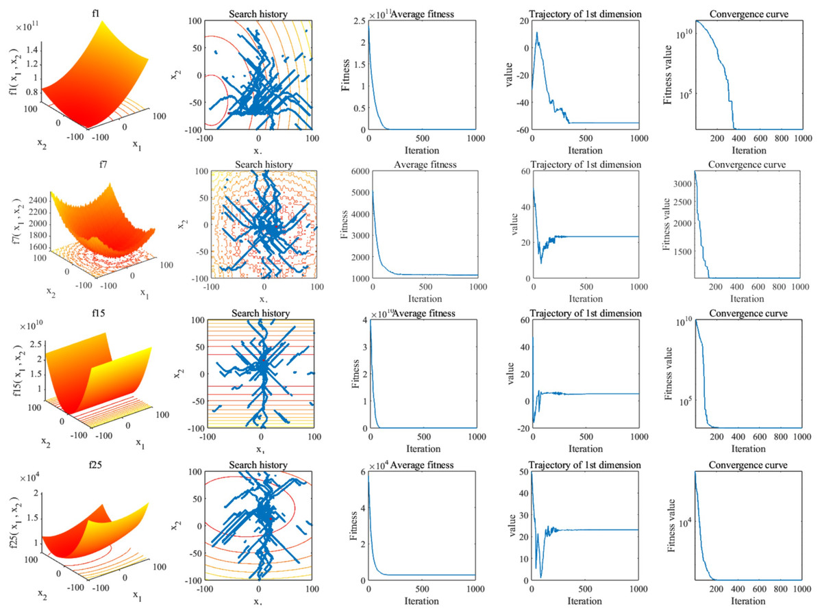
Figure 13: Curves of CBA on CEC’17 (D = 30).
From top to bottom they represent the curves of CBA of function f1, f7, f15, f25 on the CEC’17 benchmark, respectively.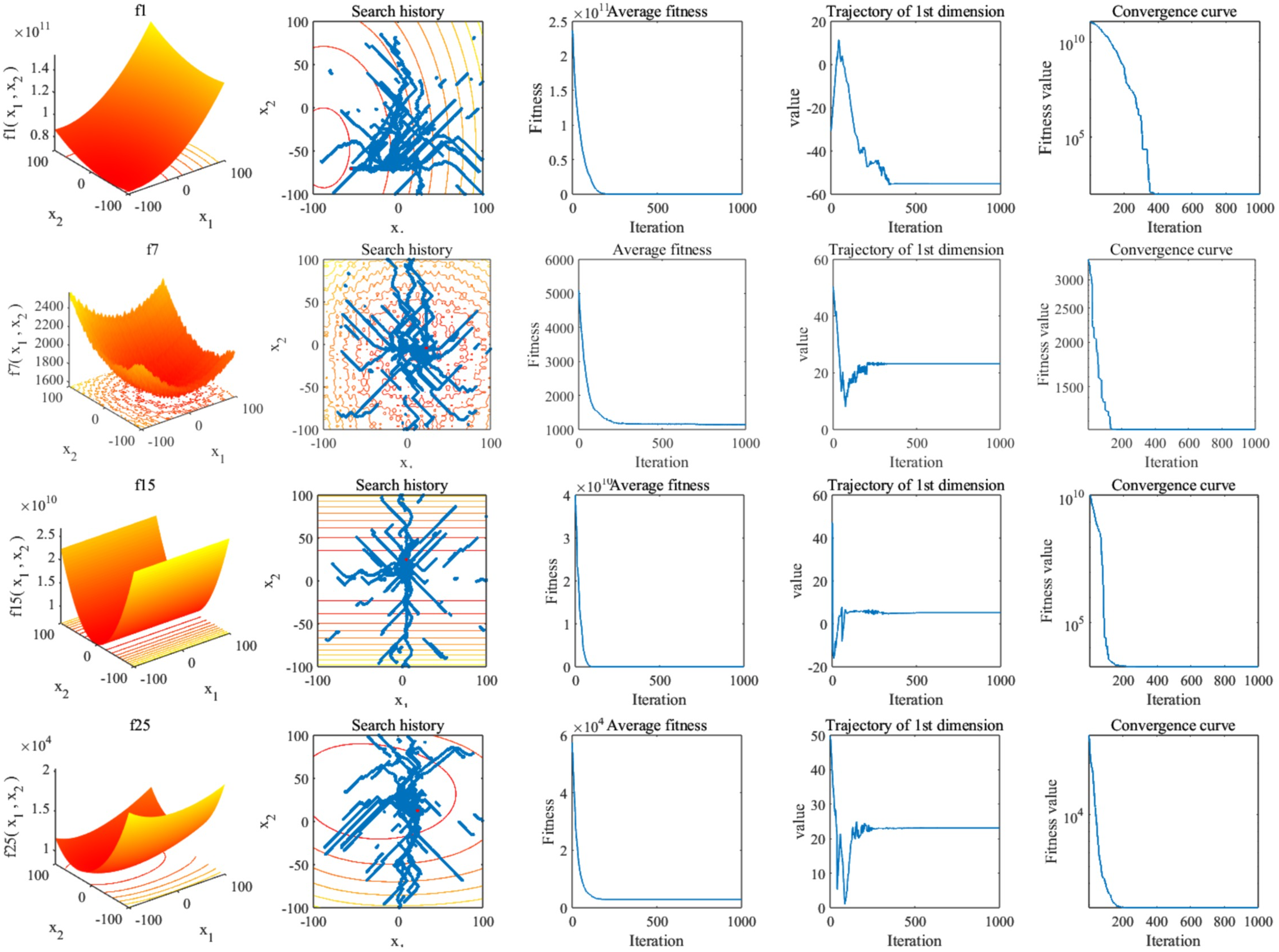
• Population Diversity Analysis (PDA): The moment of inertia in Li et al. (2023) is used to calculate swarm diversity, as seen in Eq. (17), which represents the degree of dispersion of the population around the center of mass c at each iteration, as described in Eq. (18). The parameter denotes the value of the d-th dimension of the i-th search region at iteration t (Hashim & Zamani, 2022). Without loss of generality, this scheme is adopted in this article to demonstrate the overall performance of the IDSMPSO algorithm. The formulas are described by Eqs. (17), (18):
(17)
(18)
To demonstrate the distribution breadth of particles in the solution space, Fig. 14 displays the variation of swarm diversity for four representative test functions in the 30-dimensional case, where the horizontal axis represents the number of iterations, and the vertical axis stands for population diversity. As can be seen from these figures, the swarm diversity curves of all functions exhibit a trend of rapid decline in the early stage (i.e., within 200 iterations) and gradual stabilization at a non-zero level in the later stage. The rapid decline of swarm diversity in the early evolution stage indicates that after extensively searching the solution space, particles gradually converge toward potential optimal regions and this reflects the robust exploration capability of IDSMPSO. In the later stage, the relatively low yet non-zero swarm diversity implies that the particles can not only search within the optimal regions but also retain a small number of particles to explore new areas, thus premature convergence of particles is avoided. In conclusion, IDSMPSO is able to maintain swarm diversity during the mature stage of the evolutionary search process. It is able to prevent premature convergence by exploring the search space and demonstrate great potential in finding the optimal solution.
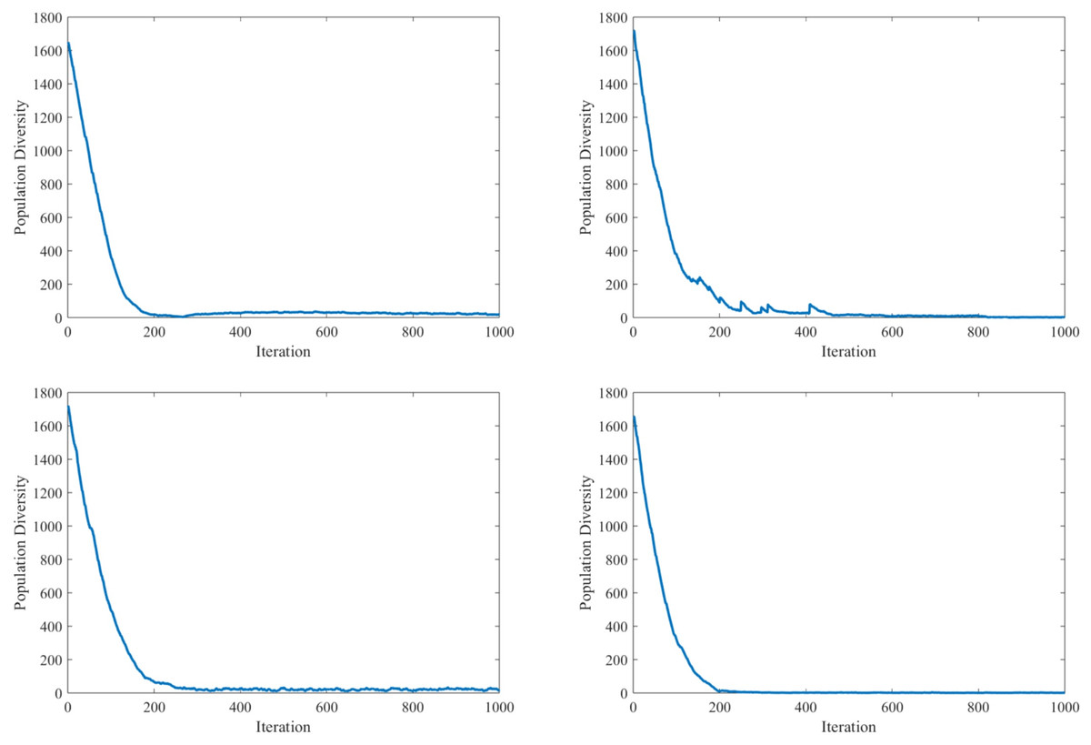
Figure 14: Curves of PDA on CEC’17 (D = 30).
From left to right and top to bottom, they represent the curves of PDA of function f1, f7, f15, f25 on the CEC’17 benchmark, respectively.
• Exploration and Exploitation Analysis (EEA): It is well known that the optimal performance of meta-heuristic algorithms depends on their ability to maintain a balance between exploration and exploitation. Typically, the percentage of exploration and exploitation changes throughout the iterations and should follow an alternating process: the red line (exploitation) rises and eventually approaches 100%, while the blue line (exploration) declines and eventually approaches 0%. This is because IDSMPSO needs to focus on exploration in the early iterations and shift towards exploitation in the later stage. Thus, we calculate the percentage of exploration and exploitation using the Eqs. (19) and (20) proposed in Li et al. (2023). The diversity measure on the dimension, Div(t), is calculated using Eq. (21), where Divmax represents the maximal diversity during the process of the entire iterations. The formulas are described by Eqs. (19)–(21):
(19)
(20)
(21)
Figure 15 illustrates the exploration and exploitation metrics obtained by IDSMPSO on four representative benchmark functions, where the horizontal axis stands for the number of iterations, and the vertical axis represents the percentage of exploration and exploitation. As can be observed from these figures, IDSMPSO can exhibit a dynamic balance between exploration and exploitation across all selected test functions. In the initial stage, the curve representing the exploration component remains at a relatively high level, while the curve for the exploitation component stays at a low level. This indicates that compared with exploitation, IDSMPSO conducts extensive exploration in the early stage of the search. However, as the number of iterations increases, an obvious transition occurs, the proportion of exploitation gradually increases, while the proportion of exploration gradually decreases. For most functions, the optimal balance between exploration and exploitation is achieved within the first 200 iterations. Notably, IDSMPSO demonstrates dynamic search behavior throughout its operation, the relationship between exploration and exploitation is balanced skillfully. This capability can enable it to outperform other methods significantly on these benchmark functions.
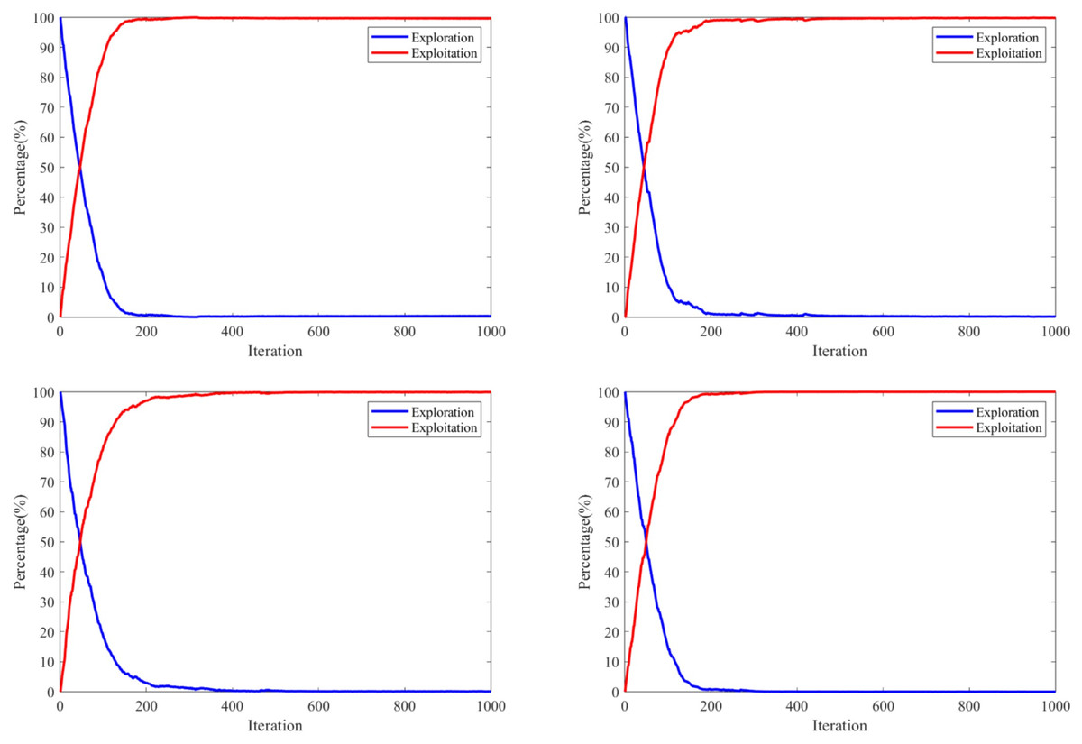
Figure 15: Curves of EEA on CEC’17 (D = 30).
From left to right and top to bottom, they represent the curves of EEA of function f1, f7, f15, f25 on the CEC’17 benchmark, respectively.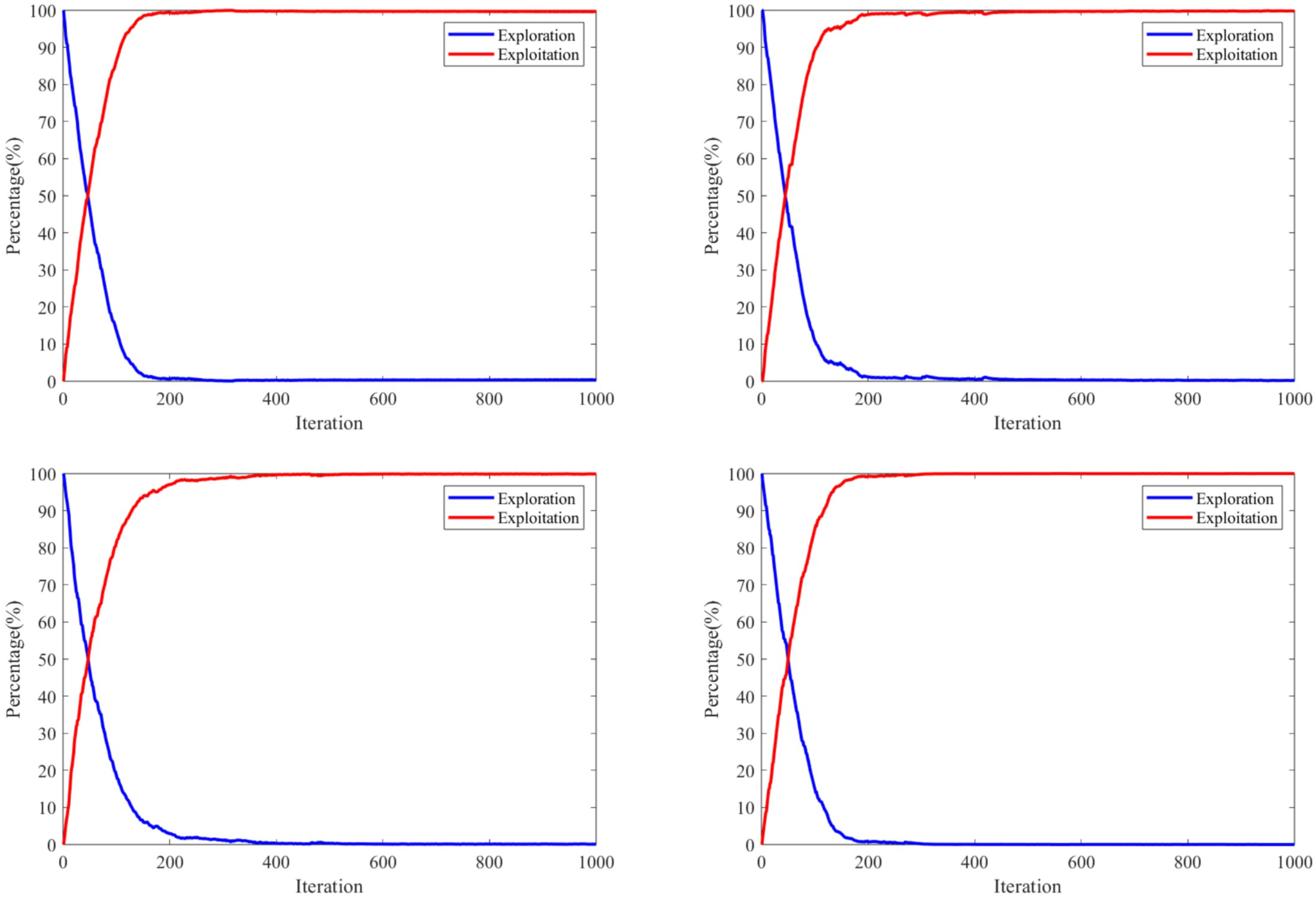
Comparison on CEC’22 test suite
In this section, experiments are conducted in 20-dimensional case. Without loss of generality, the metrics including the mean value (mv), standard deviation value (sdv), rank value (rv), average rank (AR) and final rank (FR) of the best results achieved are used to evaluate the peer algorithms. Tables 13–15 report the experimental results, and the mean value (mv), standard deviation value (sdv), rank value (rv), average rank (AR), final rank (FR) and Friedman value (f-value) of the best results are highlighted in bold.
| Func | Metric | GWO | GO | EO | KOA | MPSO | EAPSO | HPSOALS | DMPSORH | IDSMPSO |
|---|---|---|---|---|---|---|---|---|---|---|
| f1 | mv | 3.371E+04 | 1.586E+03 | 8.796E+04 | 5.675E+04 | 6.759E+02 | 6.189E+04 | 2.061E+04 | 5.338E+02 | 3.000E+02 |
| sdv | 1.011E+04 | 1.816E+03 | 5.895E+04 | 1.381E+04 | 4.116E+02 | 1.986E+04 | 6.858E+03 | 2.800E+02 | 0.000E+00 | |
| rv | 6 | 4 | 9 | 7 | 3 | 8 | 5 | 2 | 1 | |
| f2 | mv | 1.391E+03 | 4.483E+02 | 1.500E+03 | 6.959E+02 | 4.547E+02 | 5.396E+02 | 8.688E+02 | 4.569E+02 | 4.005E+02 |
| sdv | 3.867E+02 | 9.190E+00 | 5.921E+02 | 8.351E+01 | 1.104E+01 | 6.173E+01 | 2.046E+02 | 1.481E+01 | 1.490E+00 | |
| rv | 8 | 2 | 9 | 6 | 3 | 5 | 7 | 4 | 1 | |
| f3 | mv | 6.693E+02 | 6.702E+02 | 6.539E+02 | 6.433E+02 | 6.011E+02 | 6.260E+02 | 6.494E+02 | 6.517E+02 | 6.430E+02 |
| sdv | 1.174E+01 | 8.490E+00 | 1.621E+01 | 1.074E+01 | 1.620E+00 | 7.800E+00 | 9.560E+00 | 8.150E+00 | 9.740E+00 | |
| rv | 8 | 9 | 7 | 4 | 1 | 2 | 5 | 6 | 3 | |
| f4 | mv | 9.437E+02 | 8.939E+02 | 9.515E+02 | 9.776E+02 | 8.417E+02 | 9.357E+02 | 8.918E+02 | 8.912E+02 | 8.147E+02 |
| sdv | 2.025E+01 | 6.570E+00 | 1.619E+01 | 1.228E+01 | 1.603E+01 | 1.560E+01 | 2.008E+01 | 3.197E+01 | 3.360E+01 | |
| rv | 7 | 5 | 8 | 9 | 2 | 6 | 4 | 3 | 1 | |
| f5 | mv | 3.094E+03 | 2.512E+03 | 2.701E+03 | 3.016E+03 | 9.383E+02 | 1.545E+03 | 1.965E+03 | 2.247E+03 | 2.009E+03 |
| sdv | 5.075E+02 | 5.156E+01 | 5.903E+02 | 9.002E+02 | 4.559E+01 | 4.515E+02 | 3.243E+02 | 5.040E+02 | 2.492E+02 | |
| rv | 9 | 6 | 7 | 8 | 1 | 2 | 3 | 5 | 4 | |
| f6 | mv | 1.646E+08 | 4.369E+03 | 1.060E+09 | 7.606E+07 | 4.133E+03 | 4.022E+07 | 6.799E+07 | 3.802E+03 | 1.865E+03 |
| sdv | 1.887E+08 | 4.660E+03 | 1.186E+09 | 4.552E+07 | 2.090E+03 | 1.644E+07 | 1.304E+08 | 2.722E+03 | 2.345E+01 | |
| rv | 8 | 4 | 9 | 7 | 3 | 5 | 6 | 2 | 1 | |
| f7 | mv | 2.242E+03 | 2.289E+03 | 2.220E+03 | 2.214E+03 | 2.045E+03 | 2.103E+03 | 2.150E+03 | 2.152E+03 | 2.149E+03 |
| sdv | 8.232E+01 | 1.115E+02 | 1.084E+02 | 4.717E+01 | 1.753E+01 | 5.272E+01 | 4.381E+01 | 4.354E+01 | 5.077E+01 | |
| rv | 8 | 9 | 7 | 6 | 1 | 2 | 4 | 5 | 3 | |
| f8 | mv | 2.388E+03 | 2.595E+03 | 2.285E+03 | 2.300E+03 | 2.296E+03 | 2.361E+03 | 2.289E+03 | 2.333E+03 | 2.272E+03 |
| sdv | 1.497E+02 | 1.791E+02 | 7.619E+01 | 4.012E+01 | 4.727E+01 | 7.753E+01 | 6.148E+01 | 1.112E+02 | 3.737E+01 | |
| rv | 8 | 9 | 2 | 5 | 4 | 7 | 3 | 6 | 1 | |
| f9 | mv | 2.788E+03 | 2.499E+03 | 2.921E+03 | 2.576E+03 | 2.482E+03 | 2.525E+03 | 2.661E+03 | 2.487E+03 | 2.480E+03 |
| sdv | 9.657E+01 | 2.366E+01 | 2.332E+02 | 2.957E+01 | 3.160E+00 | 1.511E+01 | 6.460E+01 | 1.044E+01 | 0.060E+00 | |
| rv | 8 | 4 | 9 | 6 | 2 | 5 | 7 | 3 | 1 | |
| f10 | mv | 6.121E+03 | 5.192E+03 | 6.021E+03 | 4.263E+03 | 2.737E+03 | 5.576E+03 | 4.423E+03 | 5.089E+03 | 3.788E+03 |
| sdv | 6.015E+02 | 6.135E+02 | 1.356E+03 | 1.946E+03 | 3.728E+02 | 1.641E+03 | 1.175E+03 | 1.376E+03 | 1.199E+03 | |
| rv | 9 | 6 | 8 | 3 | 1 | 7 | 4 | 5 | 2 | |
| f11 | mv | 6..974E+03 | 2.961E+03 | 6.120E+03 | 4.553E+03 | 2.979E+03 | 1.054E+04 | 5.497E+03 | 1.619E+04 | 2.946E+03 |
| sdv | 1.002E+03 | 6.275E+01 | 1.317E+03 | 4.158E+02 | 1.080E+02 | 1.549E+03 | 9.651E+02 | 9.027E+03 | 4.465E+02 | |
| rv | 7 | 2 | 6 | 4 | 3 | 8 | 5 | 9 | 1 | |
| f12 | mv | 3.424E+03 | 3.748E+03 | 3.466E+03 | 3.066E+03 | 2.974E+03 | 2.969E+03 | 3.582E+03 | 3.784E+03 | 3.227E+03 |
| sdv | 2.634E+02 | 3.056E+02 | 3.013E+02 | 3.791E+01 | 2.535E+01 | 2.248E+01 | 2.333E+02 | 2.691E+02 | 1.697E+02 | |
| rv | 5 | 8 | 6 | 3 | 2 | 1 | 7 | 9 | 4 | |
| AR | 7.58 | 5.66 | 7.25 | 5.66 | 2.16 | 4.83 | 5.00 | 4.91 | 1.91 | |
| FR | 9 | 6 | 8 | 6 | 2 | 3 | 5 | 4 | 1 | |
| Func | Metric | GWO | GO | EO | KOA | MPSO | EAPSO | HPSOALS | DMPSORH |
|---|---|---|---|---|---|---|---|---|---|
| f1 | pv | 0.000★ | 0.000★ | 0.000★ | 0.000★ | 0.000★ | 0.000★ | 0.000★ | 0.000★ |
| hv | 1 | 1 | 1 | 1 | 1 | 1 | 1 | 1 | |
| f2 | pv | 0.000★ | 0.000★ | 0.000★ | 0.000★ | 0.000★ | 0.000★ | 0.000★ | 0.000★ |
| hv | 1 | 1 | 1 | 1 | 1 | 1 | 1 | 1 | |
| f3 | pv | 0.000★ | 0.000★ | 0.728▲ | 0.000★ | 0.000● | 0.000● | 0.464▲ | 0.000★ |
| hv | 1 | 1 | 0 | 1 | 1 | 1 | 0 | 1 | |
| f4 | pv | 0.000★ | 0.000★ | 0.000★ | 0.000★ | 0.000★ | 0.000★ | 0.000★ | 0.000★ |
| hv | 1 | 1 | 1 | 1 | 1 | 1 | 1 | 1 | |
| f5 | pv | 0.000★ | 0.000★ | 0.000★ | 0.000★ | 0.000● | 0.000● | 0.613▲ | 0.000★ |
| hv | 1 | 1 | 1 | 1 | 1 | 1 | 0 | 1 | |
| f6 | pv | 0.000★ | 0.000★ | 0.000★ | 0.000★ | 0.000★ | 0.000★ | 0.000★ | 0.000★ |
| hv | 1 | 1 | 1 | 1 | 1 | 1 | 1 | 1 | |
| f7 | pv | 0.000★ | 0.000★ | 0.019★ | 0.000★ | 0.000● | 0.000● | 0.818▲ | 0.662▲ |
| hv | 1 | 1 | 1 | 1 | 1 | 1 | 0 | 0 | |
| f8 | pv | 0.000★ | 0.000★ | 0.264▲ | 0.000★ | 0.000★ | 0.009★ | 0.001★ | 0.008★ |
| hv | 1 | 1 | 0 | 1 | 1 | 1 | 1 | 1 | |
| f9 | pv | 0.000★ | 0.006★ | 0.000★ | 0.000★ | 0.000★ | 0.000★ | 0.000★ | 0.000★ |
| hv | 1 | 1 | 1 | 1 | 1 | 1 | 1 | 1 | |
| f10 | pv | 0.001★ | 0.630▲ | 0.001★ | 0.429▲ | 0.000● | 0.000★ | 0.023★ | 0.000★ |
| hv | 1 | 0 | 1 | 0 | 1 | 1 | 1 | 1 | |
| f11 | pv | 0.000★ | 0.000★ | 0.000★ | 0.000★ | 0.000★ | 0.000★ | 0.000★ | 0.000★ |
| hv | 1 | 1 | 1 | 1 | 1 | 1 | 1 | 1 | |
| f12 | pv | 0.000★ | 0.610▲ | 0.000★ | 0.000● | 0.000● | 0.000● | 0.004★ | 0.000★ |
| hv | 1 | 0 | 1 | 1 | 1 | 1 | 1 | 1 | |
| Better (★) | 12 | 10 | 10 | 10 | 7 | 8 | 9 | 11 | |
| Same (▲) | 0 | 2 | 2 | 1 | 0 | 0 | 3 | 1 | |
| Worse (●) | 0 | 0 | 0 | 1 | 5 | 4 | 0 | 0 | |
| Func | Metric | GWO | GO | EO | KOA | MPSO | EAPSO | HPSOALS | DMPSORH | IDSMPSO |
|---|---|---|---|---|---|---|---|---|---|---|
| f1 | f-value | 6.10 | 3.33 | 8.00 | 7.73 | 2.90 | 7.80 | 5.37 | 2.77 | 1.00 |
| f2 | f-value | 8.33 | 2.30 | 8.50 | 6.03 | 3.17 | 5.10 | 7.00 | 3.57 | 1.00 |
| f3 | f-value | 7.93 | 8.20 | 5.57 | 4.27 | 1.00 | 2.37 | 5.57 | 5.80 | 2.58 |
| f4 | f-value | 6.77 | 3.50 | 7.07 | 8.67 | 1.87 | 6.20 | 3.33 | 3.40 | 1.03 |
| f5 | f-value | 7.63 | 5.90 | 6.23 | 6.87 | 1.00 | 2.37 | 3.63 | 4.57 | 3.71 |
| f6 | f-value | 7.67 | 2.97 | 7.80 | 7.30 | 3.17 | 6.40 | 5.77 | 2.93 | 1.00 |
| f7 | f-value | 6.57 | 7.37 | 5.73 | 6.53 | 1.67 | 2.03 | 3.63 | 3.93 | 2.41 |
| f8 | f-value | 6.50 | 8.13 | 4.40 | 5.20 | 1.93 | 6.67 | 3.20 | 5.20 | 1.77 |
| f9 | f-value | 8.27 | 3.67 | 8.47 | 6.13 | 2.00 | 4.97 | 7.07 | 2.97 | 1.47 |
| f10 | f-value | 7.00 | 5.27 | 7.43 | 4.63 | 1.87 | 6.73 | 4.07 | 5.07 | 2.43 |
| f11 | f-value | 6.53 | 2.53 | 5.73 | 4.37 | 2.37 | 8.30 | 5.23 | 8.70 | 1.23 |
| f12 | f-value | 5.87 | 7.67 | 6.10 | 2.97 | 1.74 | 1.17 | 6.87 | 7.80 | 4.00 |
| AR | 7.09 | 5.07 | 6.75 | 5.89 | 2.05 | 5.00 | 5.06 | 4.72 | 1.96 | |
| FR | 9 | 6 | 8 | 7 | 2 | 4 | 5 | 3 | 1 | |
Accuracy comparison
To further demonstrate the superiority of IDSMPSO, we conduct additional experiments where eight peer algorithms are compared against our proposed IDSMPSO in the 20-dimensional space of CEC’22. Table 13 presents the experimental results of the aforementioned nine algorithms. Specifically, IDSMPSO achieves the 1st rank in seven functions, the 2nd rank in one function, the 3rd rank in two functions, and the 4th rank in two functions. Ultimately, it still maintains the 1st position in terms of average ranking. As shown in the table, IDSMPSO exhibits the best performance on unimodal functions. It also performs well on multimodal functions, securing the 1st rank on functions f2 and f4. For the three hybrid functions, IDSMPSO delivers excellent results, it ranks 1st on two of the three hybrid functions and 3rd on function f7. In terms of the four composite functions, IDSMPSO also shows good performance, which achieves the 1st rank on functions f9 and f11, and the 2nd rank on function f10. Overall, IDSMPSO validates high performance on both unimodal and hybrid functions, with particularly excellent performance on unimodal functions.
Convergence speed comparison
To test the convergence speed of the nine algorithms, Fig. 16 presents the convergence curves of four representative functions (f1, f2, f6, f9). Overall, although the convergence speed of IDSMPSO is not the fastest, IDSMPSO can steadily maintain the smallest fitness value compared with other algorithms as iterations proceed. Taking f1 as an example, in the first 100 iterations, all peer algorithms exhibit extremely fast convergence rate. After that, except for MPSO, DMPSORH, GO and IDSMPSO, the fitness values of other algorithms remain almost unchanged in the subsequent iterations. In contrast, IDSMPSO is able to speed up the convergence process during the 100–300 iterations, and thereafter maintains a stable fitness value, which is better than that of other peer algorithms. But, in the light of the “No Free Lunch” theorem (Wolpert & Macready, 1997), for f9, IDSMPSO’s convergence accuracy only surpasses that of all peer algorithms around 400 iterations. In conclusion, IDSMPSO has obtained higher performance across different types of benchmark functions.
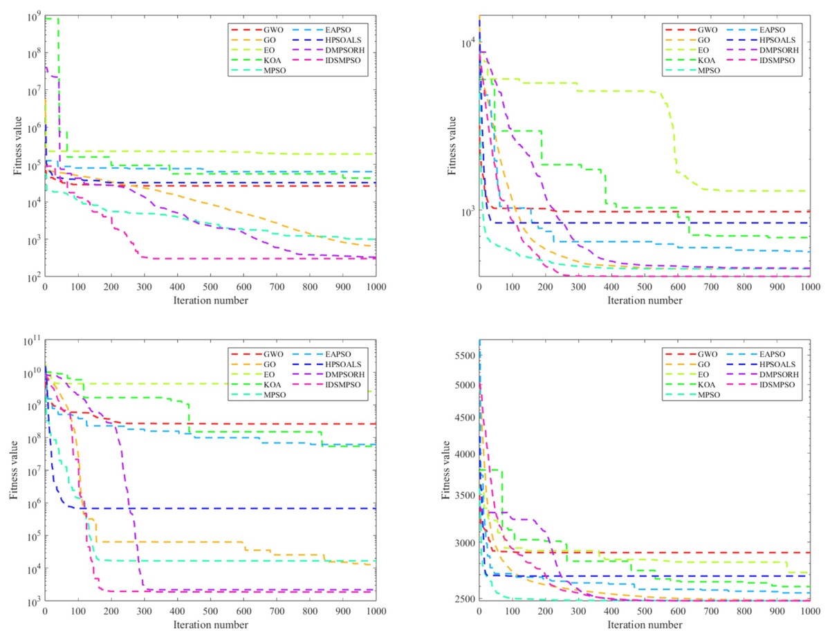
Figure 16: Convergence curves of IDSMPSO and the compared algorithm on CEC’22 (D = 20).
From left to right and top to bottom, they represent the convergence curves of function f1, f2, f6, f9 on the CEC’22 benchmark, respectively.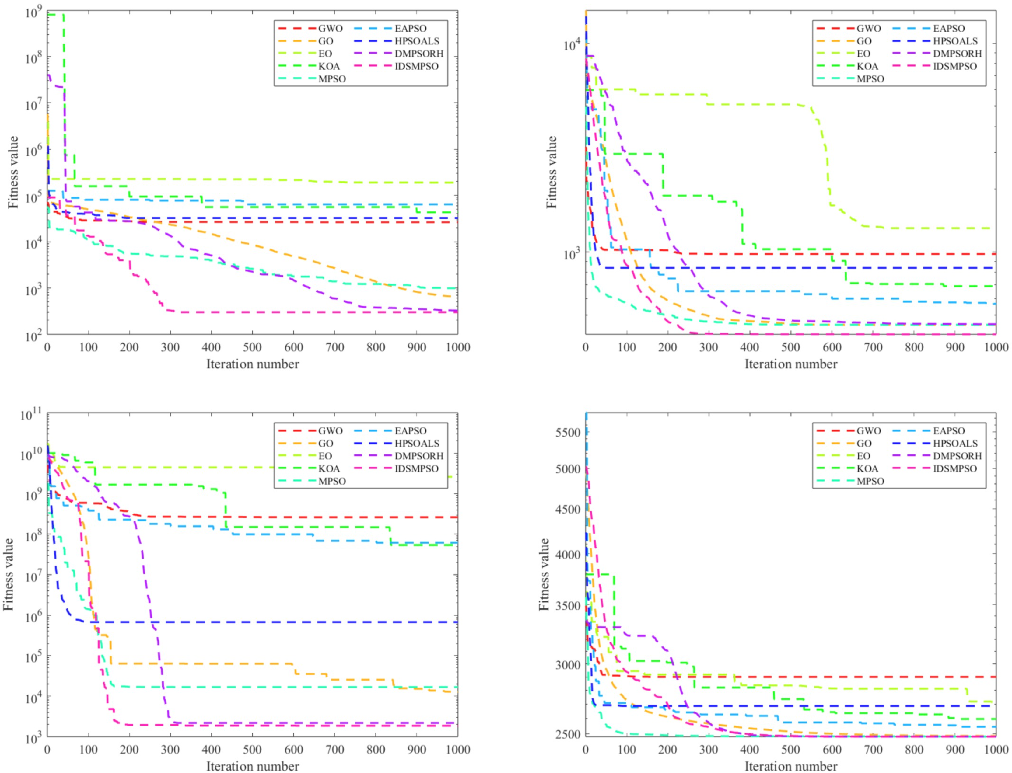
Non-parametric statistical tests
To bear out the significant differences between IDSMPSO and other algorithms, Table 14 presents the test results of 20-dimensional cases from the CEC’22 test suite. IDSMPSO shows significant advantages over GWO, GO, EO, KOA, HPSOALS and DMPSORH. Specifically, IDSMPSO outperforms the aforementioned peer algorithms on 12, 10, 10, 10, 9 and 11 test functions respectively. However, KOA only performs comparably to IDSMPSO on one test function each (namely f10). When compared with the other two algorithms (i.e., MPSO and EAPSO), IDSMPSO still maintains its superiority, it surpasses them on 7 and 8 functions respectively, though it is slightly inferior to them on 5 and 4 functions each. In conclusion, IDSMPSO is able to perform better than other peer algorithms on at least half of the test functions.
The stability of IDSMPSO is verified using CEC’22 test suite under 20-dimensional case. Four representative functions are selected for experiment, and their results are illustrated in Fig. 17 to validate the stability of IDSMPSO. For function f1, outliers are observed in the results of GO, EO, KOA, MPSO, HPSOALS and DMPSORH. In contrast, IDSMPSO can achieve high convergence accuracy and exhibits the best stability. Regarding f2, MPSO and EAPSO perform well, with no outliers detect in their results. For function f6, HPSOALS shows a relatively large number of outliers, while other peer algorithms maintain good stability. As for function f9, IDSMPSO attains the highest convergence accuracy among all compared methods. In a word, IDSMPSO has achieved higher convergence accuracy and better algorithmic stability in contrast with other peer approaches.
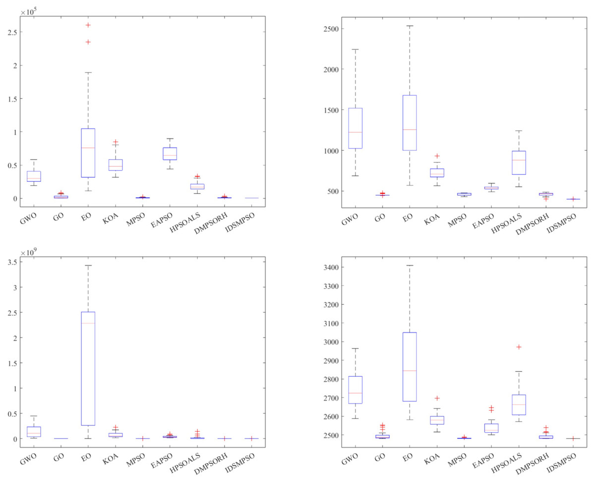
Figure 17: Boxplot for different algorithms on CEC’22 (D = 20).
From left to right and top to bottom, they represent the boxplot of function f1, f2, f6, f9 on the CEC’22 benchmark, respectively.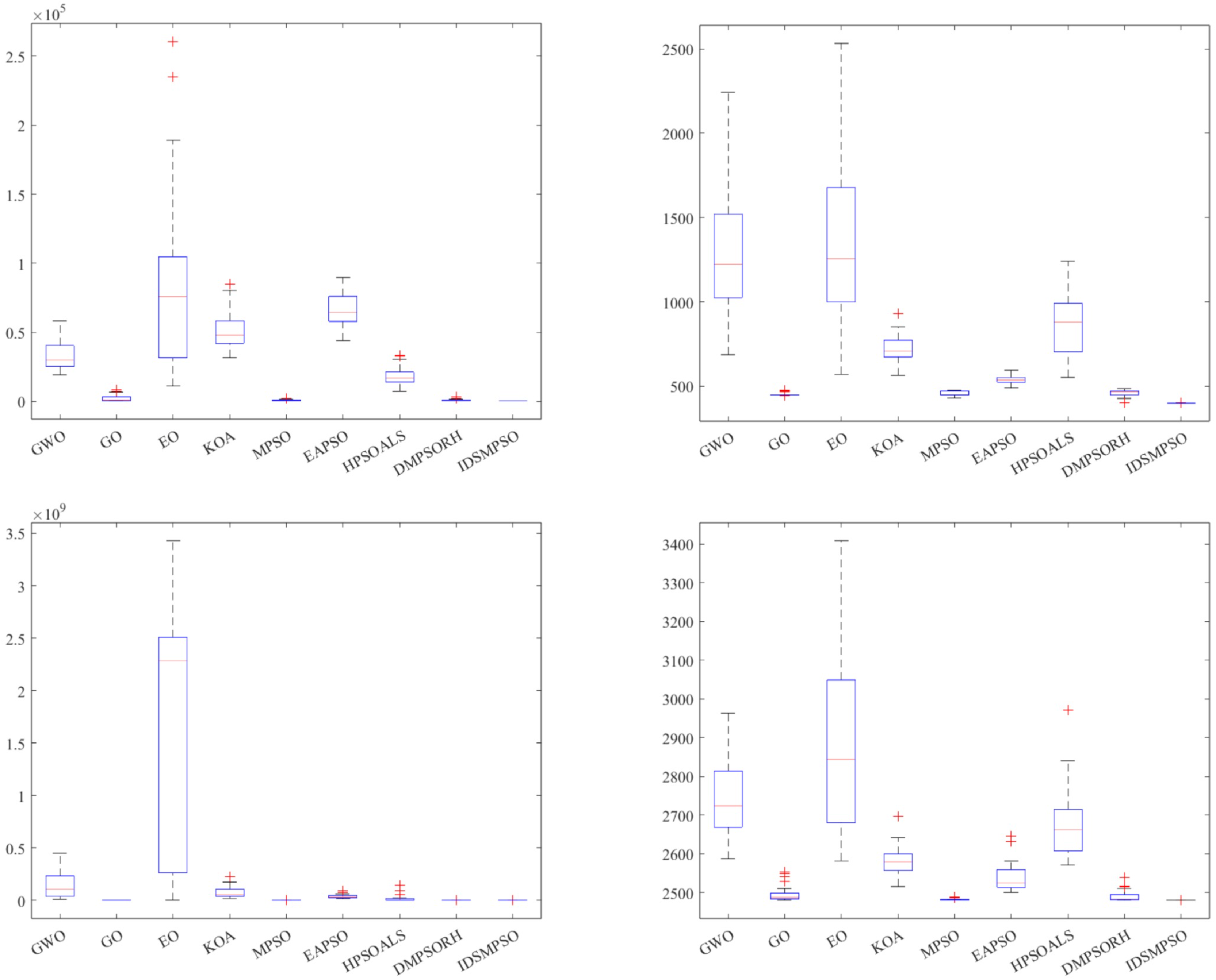
To conduct a more detailed analysis of our proposal, the Friedman test is performed in the 20-dimensional case. Table 15 shows that IDSMPSO also performs excellently, followed by MPSO, DMPSORH, EAPSO, HPSOALS, GO, KOA, EO and GWO.
Application in real-world problems
Three-dimensional UAV path planning is a crucial technology involving the design of optimal flight paths in three-dimensional space to ensure that unmanned aerial vehicles (UAV) avoid obstacles while flying from a starting point to a target point. This technology not only needs to ensure the safety of the UAV, but also optimize the efficiency of the path, typically targeting the shortest flight time, minimal energy consumption, or the shortest distance. To assist the UAV in finding the optimal path, this work applies the IDSMPSO algorithm for optimization and compares its performance with other competitive algorithms (GWO, GO, EO, KOA, DMPSORH, HPSOALS). The research is introduced from four aspects of the simulation environment, path evaluation and constraints, collision detection and the shortest path. We implemented the proposed IDSMPSO in MATLAB 2022B. The experiments are carried out on the platform of 3.20 GHz AMD Ryzen CPU computer with 32.0G memory running Win 11 professional systems.
Simulation environment
To achieve path planning, the environmental model is used in Huang et al. (2021) to simulate complex peaks. The environmental information needed for 3D path planning is extracted from a terrain model, in which natural peaks in the flight environment are described using an exponential function. Its mathematical model can be expressed by Eq. (22):
(22) where n represents the total number of peaks, hi is the terrain parameter controlling peak height, and (xi, yi) represent the coordinates of the center of the i-th peak. xsi and ysi are the decay factors along the x-axis and y-axis, respectively, controlling the slope of the peak. The relevant terrain parameters are shown in Table 16. x, y, and z correspond to the horizontal, vertical, and height dimensions respectively, with the unit of meter.
| Parameter category | Specific description |
|---|---|
| Map range | 200 × 200 × 300 (x ∈ [0, 200], y ∈ [0, 200], z ∈ [0, 300]) |
| Number of mountains | 15 |
| Mountain distribution | x ∈ [10, 190], y ∈ [10, 190] |
| Height range | [60, 300] |
It’s worth noting that the start and end points of the UAV path are fixed at coordinates (1, 1, 1) and (180, 180, 160), respectively. This diagonal layout of the start and end points is intentionally designed to create a path planning task that covers the main area of the terrain. For the specific representation of the UAV path, a hybrid approach combining “discrete nodes and cubic spline interpolation” is employed: First, three intermediate nodes (excluding the pre-fixed start and end points) are designated as core control points for path optimization, with their coordinates determined through the iterative search of optimization algorithms. Subsequently, cubic spline interpolation is applied to the complete set of discrete nodes (i.e., the starting point, three intermediate nodes, and end point). This interpolation process generates a continuous path with a large number of sampling points. For the sake of fairness, all peer algorithms are tested using identical parameters. The parameters involved are presented in Table 17.
| Parameter category | Specific description |
|---|---|
| Population size | 30 |
| Maximum iterations | 100 |
| Variable dimension | 15 |
| Number of independent experiments | 30 |
| Random seed | rng (3) |
Path evaluation and constraints
We take the total path length (L) as its fitness value to evaluate the flight results. This evaluation index is represented by Eq. (23):
(23) where (xi, yi, zi) represents the 3D coordinates of the i-th sampling point on the path, n denotes the total number of sampling points on the path. Meanwhile, a collision penalty mechanism is implemented based on the above. If the path collides with the terrain, the fitness value (L) is multiplied by a penalty factor of 1,000 to ensure the algorithm prioritizes collision-free paths. Collisions are determined by two key conditions: one is whether any sampling point on the path lies outside the terrain range or not, and the other is whether the difference between the terrain elevation at their corresponding position and the sampling point’s own height exceeds a preset safety margin for sampling points or not within the terrain range. It is worth noting that our safety margin is set to 0.5 m. In addition, there are two constraint variables for the search space as follows. The lower bound of search (lb) is set such that the minimal value of all coordinate dimensions is 1, whose purpose is to avoid indexing issues that may arise when the coordinate value is 0. For the upper bound of search (ub), the maximal values of the x-direction, y-direction and z-direction are set to 199, 199 and 299, respectively. As a result, the formed search space is [1,199] × [1,199] × [1,299].
Collision detection
Based on the aforementioned path evaluation method, quantitative data (average fitness value, the number and rate of collisions) for the seven algorithms are supplemented to highlight performance differences in short-distance, cross-elevation scenarios. It is worth noting that the straight-line distance from the starting position to the target position is 298.94. Table 18 presents the results of peer algorithms (GWO, GO, EO, KOA, DMPSORH, HPSOALS) and our proposal based on 30 independent runs. The average fitness represents the mean of the sum of all fitness values, regardless of path collision status. From Table 18, it is obvious that IDSMPSO proposed in this article exhibits the superior performance, followed by EO, DMPSORH, GWO, HPSOALS, GO and KOA.
| Algorithm | Number of collisions | Collision rate | Average fitness | Rank |
|---|---|---|---|---|
| GWO | 20 | 66.67 | 2.199E+05 | 4 |
| GO | 27 | 90.00 | 2.742E+05 | 6 |
| EO | 18 | 60.00 | 1.811E+05 | 2 |
| KOA | 25 | 83.33 | 4.275E+05 | 7 |
| DMPSORH | 13 | 43.33 | 1.946E+05 | 3 |
| HPSOALS | 26 | 86.66 | 2.739E+05 | 5 |
| IDSMPSO | 6 | 20.00 | 6.955E+04 | 1 |
Comparison of the shortest path
In this section, we will further demonstrate the superiority of IDSMPSO in UAV path planning based on the following experimental results. Note that we select the collision-free path that is the best among the 30 runs, and rhombus denotes the start point of the path whereas triangle stands for the end point. Our ultimate goal is to evade all the peaks and discover the optimal route. As can be seen from Figs. 18 and 19, IDSMPSO performs better than other peer methods in finding the global optimal solution.
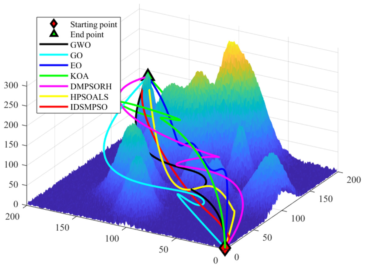
Figure 18: Main view of each peer algorithm for the shortest paths.
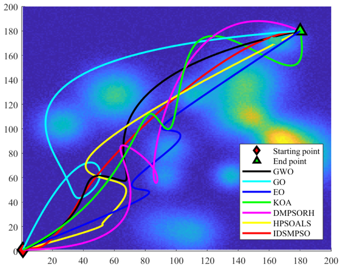
Figure 19: Top view of each peer algorithm for the shortest paths.
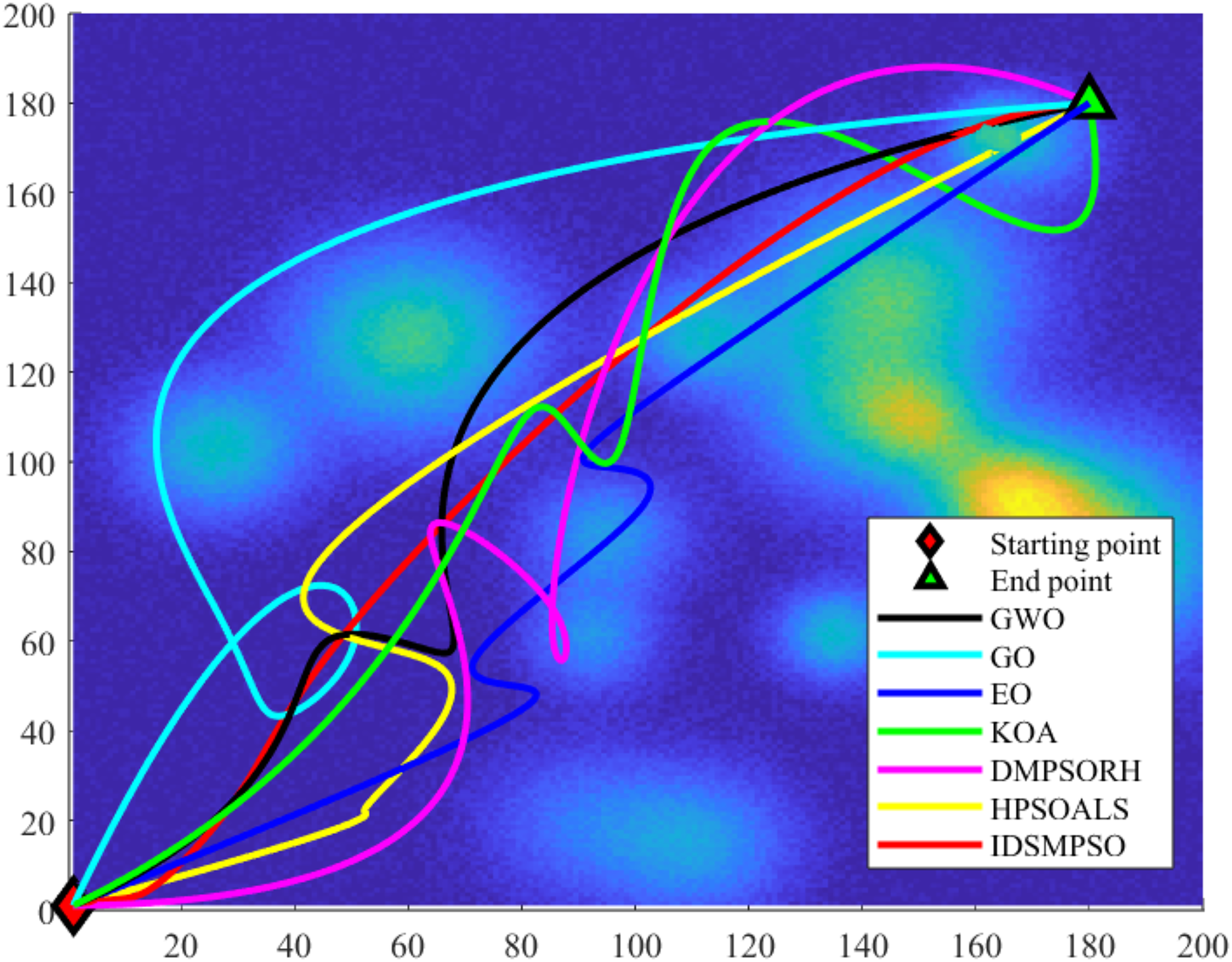
Besides, Table 19 reports changes of the fitness values for each peer algorithm as the number of iterations increases. These values are recorded at 0, 20, 40, 60, 80 and 100 iterations. By the 100th iteration, IDSMPSO has achieved the lowest value (298.96), followed closely by GO at 302.46. In sum, it can be clearly observed that IDSMPSO surpasses other peer algorithms in terms of searching ability. Subsequently, GO shows slightly inferior convergence compared to IDSMPSO but still can achieve favorable optimization results. They are followed by HPSOALS, GWO, EO, DMPSORH and KOA. Alternatively, Fig. 20 illustrates the convergence process of them to further validate the superiority of our proposal.
| Iteration | 0 | 20 | 40 | 60 | 80 | 100 |
|---|---|---|---|---|---|---|
| GWO | 449.10 | 319.34 | 319.32 | 319.309 | 319.308 | 319.30 |
| GO | 747.82 | 322.85 | 311.11 | 306.33 | 303.72 | 302.46 |
| EO | 551.60 | 454.58 | 392.68 | 392.24 | 369.78 | 343.22 |
| KOA | 627.69 | 627.69 | 627.69 | 627.69 | 627.69 | 465.33 |
| DMPSORH | 854.07 | 745.43 | 738.79 | 583.34 | 486.67 | 369.62 |
| HPSOALS | 753.98 | 316.65 | 304.42 | 303.25 | 303.24 | 303.23 |
| IDSMPSO | 758.12 | 318.58 | 301.03 | 299.13 | 298.97 | 298.96 |
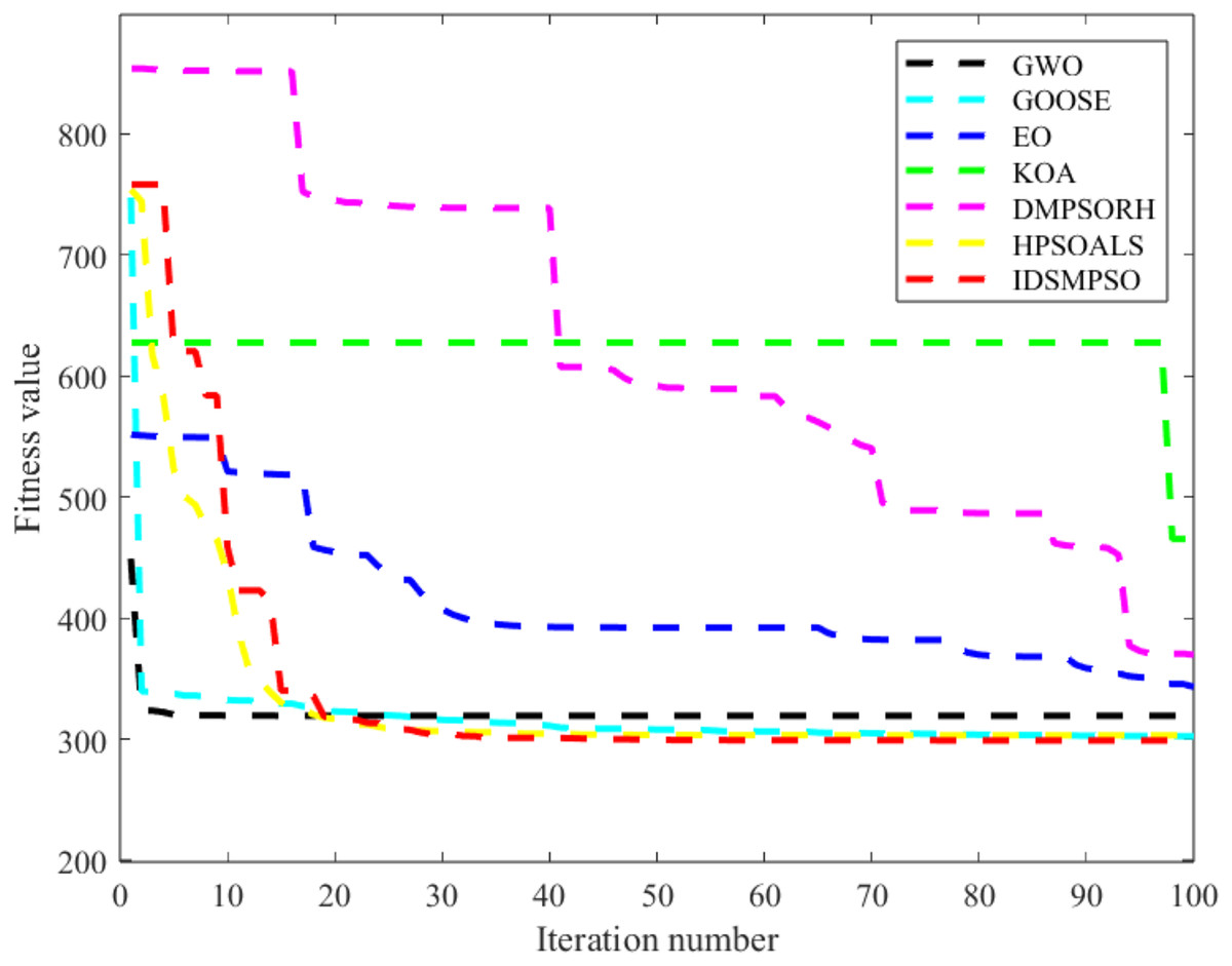
Figure 20: Convergence curves of each peer algorithm for the shortest path.
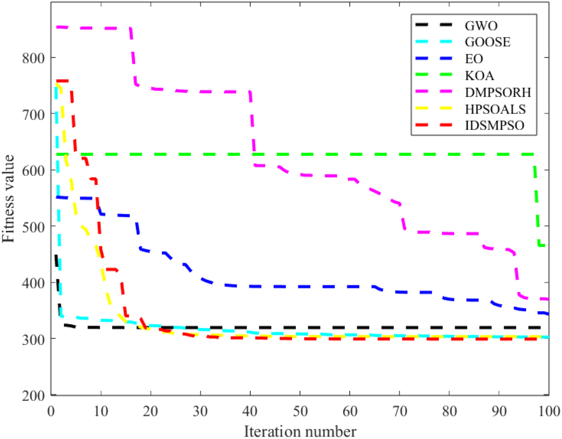
Conclusion and future work
To address the shortcomings of PSO, such as local optima and slow convergence, IDSMPSO is proposed in this article. The main contributions of it can be summarized as: I. Dynamic sub-swarm division: unlike traditional fixed-sized subgroup methods, IDSMPSO divides the global swarm into four subgroups (best, better, worse, worst) based on particles’ fitness values with the number of particles in each subgroup varying randomly across. This dynamic adjustment strategy can effectively sustain the swarm diversity. II. Adaptive inertia weight: different subgroups use different inertia weight strategies and each particle has its own inertia value, which is able to enhance the convergence speed of swarms significantly. III. Different learning strategies for different subgroups: various classical learning strategies are employed in each sub-swarm to strengthen the optimization performance, including the elite learning, cooperative learning and greedy strategy. IV. BFGS quasi-newton method: the BFGS quasi-Newton method is used to refine the optimal solution to strengthen the exploitation capability. Besides, to demonstrate the optimization performance of IDSMPSO, extensive experiments are conducted on CEC’17 and CEC’22, and the experimental results show that our proposal outperforms other peer algorithms. Moreover, IDSMPSO is applied to 3-D UAV path planning problem and it has also obtained promising results.
However, one of the limitations of IDSMPSO is its poor convergence accuracy and convergence speed when it is applied to multimodal functions. This is expected as especially in the light of “No Free Lunch” theorem, there is no general-purpose optimization algorithm which can solve all classes of problems and all the algorithms have pros and cons on solving optimization problems. Secondly, IDSMPSO is more complex compared to other PSOs and it requires additional computations. However, the computational resources are mostly spent on the evaluating of the objective functions. Hence, the additional computational requirement of the optimization strategy for IDSMPSO is negligible. Besides, IDSMPSO offers faster convergence rate and this can be translated into additional saving on computation time.
In the future, we aim to further promote the performance of IDSMPSO from the following directions: refine the population division method to enhance swarm diversity, adjust the inertia weight in each subgroup for better performance, adopt more efficient learning strategies to improve the information exchange between subgroups and integrate the archive strategy into IDSMPSO to further accelerate the convergence process of subgroups. Additionally, we plan to apply IDSMPSO to other fields, such as feature selection and engineering optimization in order to further demonstrate its effectiveness.