Brain disease diagnosis using federated deep learning

Mustafa Abdul Salam; Omnia Atef; Nabil Abdel Salam; Mohammed Aldawsari

doi:10.7717/peerj-cs.3545

Brain disease diagnosis using federated deep learning

Mustafa Abdul Salam ¹, Omnia Atef², Nabil Abdel Salam³, Mohammed Aldawsari¹

1Department of Computer Engineering and Information, College of Engineering in Wadi Addwasir, Prince Sattam Bin Abdulaziz University, Wadi Addwaser, Saudi Arabia

2Computer Science, Egyptian E-Learning University, Giza, Egypt

3Computer Science, Higher Technological Institute, Tenth of Ramadan City, Egypt

DOI: 10.7717/peerj-cs.3545

Published: 2026-02-02
Accepted: 2025-12-09
Received: 2025-09-26

Academic Editor: Nicole Nogoy

Subject Areas: Artificial Intelligence, Computer Vision, Data Mining and Machine Learning, Data Science, Neural Networks
Keywords: Federated learning, MGMT, Convolutional neural network, Recurrent neural network, Swarm intelligence, Bayesian search, Sparrow search

Copyright: © 2026 Abdul Salam et al.
Licence: This is an open access article distributed under the terms of the Creative Commons Attribution License, which permits unrestricted use, distribution, reproduction and adaptation in any medium and for any purpose provided that it is properly attributed. For attribution, the original author(s), title, publication source (PeerJ Computer Science) and either DOI or URL of the article must be cited.

Cite this article: Abdul Salam M, Atef O, Abdel Salam N, Aldawsari M. 2026. Brain disease diagnosis using federated deep learning. PeerJ Computer Science 12:e3545 https://doi.org/10.7717/peerj-cs.3545

The authors have chosen to make the review history of this article public.

Abstract

Brain tumors often require treatment and multiple biopsies. They are the third most common cancer among young adults in both incidence and mortality. The expression of the O6-methylguanine-DNA methyltransferase (MGMT) gene plays an important role in predicting tumor behavior. It affects how patients respond to chemotherapy and may reduce the need for invasive procedures. Machine learning can help make accurate medical predictions, but it requires large and diverse patient datasets. These datasets are difficult to access due to privacy and legal restrictions. This article proposes a Federated Learning (FL) framework to address these challenges. FL allows different institutions to train a shared model without exchanging raw data. A hybrid deep learning model combining recurrent neural networks (RNNs) and convolutional neural networks (CNNs) is developed to analyze magnetic resonance imaging (MRI) scans from the BraTS 2021 dataset. The model aims to detect glioblastoma and predict MGMT gene expression. Two swarm intelligence algorithms, the Bayesian Search Optimization Algorithm and the Sparrow Search Optimization Algorithm, are used to optimize the model’s hyperparameters. The FL system was tested across ten universities. It performed similarly to models trained on centralized data. The proposed model, BrainGeneDeepNet, achieved high performance: 0.9758 accuracy, 0.0769 loss, 0.9980 AUC, 0.9770 recall, and 0.9782 precision. These results show that federated learning is a secure and effective approach for medical imaging and biomarker prediction.

Introduction

With billions of cells, the brain is the most intricate organ in the human body. When cells divide uncontrollably and form an aberrant group, a brain tumor develops. In certain situations, the set of cells can cause death, damage healthy cells, or interfere with regular brain activity. In recent years, brain tumors classified as one of the major causes of growing death rates (Logeswari & Karnan, 2010; Kavitha & Kanaga, 2016; El Abbadi & Kadhim, 2017).

The size, shape, location, and picture intensity of brain tumors vary. There are more than 100 primary categories of brain tumors. But not every brain tumor—or even every malignant brain tumor—is lethal. Many tumor types respond well to chemotherapy, radiation therapy, and surgery, and they may even be cured. However, surgical resection is not usually effective in curing many of the more common tumors, like gliomas (Das & Rajan, 2016).

However, the World Health Organization (WHO) developed the most popular grading system available today, which divides brain tumors into classes I through IV based on behavior and increasing aggressiveness. Because they grow rather quickly, malignant tumors are classified as grade III or IV. Early detection and diagnosis can aid in the treatment plan or lower the likelihood that the tumor would return following surgical removal. The Central Brain Tumor Registry of the United States (CBTRUS) ranked brain tumors as the third most common cancer among young adults (ages 15–39), and the National Cancer Institute Statistics (NCIS) in the United States show that the overall incidence of cancer, including brain cancer, has increased by more than 10% over the past 20 years.

The tumor’s reaction to chemotherapy is really correlated with the existence of a certain genetic sequence in the tumor called O6-methylguanine-DNA methyltransferase (MGMT) promoter methylation. A protein called MGMT fixes damage to human body cells’ DNA. Tumor cells are harmed by the chemotherapy medications. Therefore, it is anticipated that the chemotherapy treatment will be less effective the more MGMT protein the tumor generates since the protein will heal the damage to the tumor. Currently, MGMT identification necessitates a biopsy, which can take several weeks and involves taking tissue from the tumor and analyzing it. Further surgery may be required, depending on the outcomes and the kinds of treatments initially used. The frequency of procedures may be reduced if an effective detection technique using medical imaging (such as MRI and radiogenomics) is developed (Feldheim et al., 2019; Mansouri et al., 2019; Yu et al., 2019; Häni et al., 2022).

A number of different areas and applications have used machine learning and artificial intelligence in recent years to extract meaningful relationships and make accurate predictions. The key reason is that they provide the ability to refine models and learn from the experience by using the input data and producing new predicted output values. Healthcare is a very critical area that requires large amounts of sensitive data. The training model used in this field collects data from different data islands, posing a risk to patient data privacy, which constitutes an obstacle to the overall progress of artificial intelligence in the fields of healthcare and life sciences (Wang, Casalino & Khullar, 2019; Chartrand et al., 2017; De Fauw et al., 2018; Sun et al., 2017).

The reliance on traditional artificial intelligence (AI) techniques requires data sharing with the centralized server which threatens patient privacy due to the natural sensitivity of healthcare informatics. Indeed, sharing of data in a centralized server increase the occurrence of unauthorized access and gives the chance to control the data and modify data patterns without the consent of users. Although the centralized servers can provide efficient data training and analysis by virtue of their powerful computational capabilities, these bottlenecks would result in information leakage (Yang & Liu, 2020).

To eliminate sharing patient data with a centralized server we need to train the model locally at each medical institution. On the other hand, AI-based models require a huge amount of data for the learning process, and only one medical site has its own data, which is not enough to train the model. This results in reliance on manual data analyses, but this incurs a long time for data processing. Hence, dataset shortage is a very critical issue in healthcare system development. The insufficient training of the AI-based model cannot achieve the desired degree of classification accuracy due to the lack of datasets at the medical site. This makes the training process more difficult (Atef, Salam & Abdelsalam, 2022).

The data types of healthcare informatics are usually image and audio with a large size which increases the data offloading time to the central server and requires more transmission power and hardware prerequisites for user devices. Moreover, data transferring also consumes much network bandwidth, which may cause congestion in the network when the number of users increases (Zhang, Bosch & Holmström Olsson, 2020).

The addressed challenges show the need for a new approach to enable each medical institution to efficiently train a machine learning model using their own data locally without sharing it with others and preserving the privacy of patients.

The remainder of this article is structured as follows: ‘Related Work’ presents works relating to predicting the MGMT gene using classical and federated learning. ‘Preliminary’ presents a description of the architecture of the federated learning approach followed by an explanation of the algorithms used in swarm intelligence. The proposed model architecture is demonstrated in ‘Proposed Model’, while experimental results are discussed in ‘Experimental Setup’. Finally, ‘Conclusion and Future Work’ concludes our work.

Related work

Recent work has shown that swarm-driven and bio-inspired optimization strategies can significantly enhance accuracy and generalization when applied to deep learning frameworks for brain tumor detection and classification (Saifullah et al., 2025; Yonar, 2025; Agrawal et al., 2025). As a result, the fusion of deep neural architectures with nature-inspired optimization is emerging as a powerful paradigm for developing intelligent diagnostic systems capable of handling high-dimensional imaging data and improving clinical decision-making in brain disease diagnosis (Saifullah et al., 2025; Agrawal et al., 2025).

Recent research has shown that federated deep learning (FL) is becoming a promising solution for brain disease diagnosis, especially in environments where data privacy and multi-institutional collaboration are essential. Wen et al. (2025) proposed a generalized FL framework for brain tumor segmentation that integrates virtual adversarial training and a 3D U-Net model, demonstrating improved generalization across heterogeneous MRI datasets from multiple clinical sites. Similarly, Onaizah, Xia & Hussain (2025) introduced FL-SiCNN, a privacy-preserving federated deep learning model that enhances brain tumor classification accuracy while reducing communication overhead, showing better efficiency compared to conventional centralized learning approaches. Another study by Albalawi et al. (2024) demonstrated that combining federated learning with transfer learning enables high-accuracy multi-class brain tumor diagnosis across distributed healthcare centers without compromising patient confidentiality. Additionally, Ma (2025) provided a comprehensive analysis of emerging FL applications in brain tumor diagnosis, highlighting improvements in robustness, data fairness, and deployment readiness in real-world clinical settings. Collectively, these recent works illustrate how federated deep learning is transitioning from experimental architecture concepts to practical medical AI systems capable of supporting scalable, privacy-aware brain disease diagnosis.

In recent years, a number of machine learning methods have been created with promising results to classify the methylation state of the MGMT promoter.

In order to predict MGMT methylation status without requiring a separate tumor segmentation phase, (Korfiatis et al., 2017) trained three independent residual deep neural networks, ResNet18, ResNet34, and ResNet50 architectures. using T2 and T1 weighted post-contrast MR scans from the Mayo Clinic. With an accuracy of 94.90%, the ResNet50 was the top-performing model (Chen et al., 2022).

Using contrast-enhanced T1W images and fluid-attenuated inversion recovery images (FLAIR) from 87 glioblastoma patients, Chen et al. (2022) created a deep learning pipeline for the automatic prediction of MGMT status. Both tumor segmentation and status categorization were successful with the suggested approach. FLAIR images perform better in tumor segmentation (Dice score of 0.897) than contrast-enhanced T1WI (Dice score of 0.828). Additionally, FLAIR images perform better in status prediction (accuracy score of 0.827, recall score of 0.852, precision score of 0.821, and F1-score of 0.836). The suggested workflow achieves a good prediction of MGMT methylation status while cutting down on tumor annotation time and eliminating interrater variability in glioma segmentation. Treatment planning would then be made easier by the identification of molecular biomarkers from routine medical pictures (Yogananda et al., 2021).

In a different study, Yogananda et al. (2021) created the MGMT-net, a T2WI-only network that is utilized to identify MGMT methylation status and segment tumors, based on 3D-Dense-UNets. They reported a cross-validation accuracy of 94.73% across three folds with a sensitivity score of 96.31% and a specificity score of 91.66% using MRI images from the TCIA and TCGA datasets (Chen et al., 2020).

Chen et al. (2020) used MRI scans from 111 patients to predict the MGMT promoter methylation using a deep-learning method based on ResNet18 with five-fold cross-validation. T1 weighted image (T1WI), T2 weighted image (T2WI), apparent diffusion coefficient (ADC) maps, and T1 contrast-enhanced (T1CE) for four sequence types are the radionics features of the two regions of interest (ROI) (the entire tumor area and the tumor core area). The average accuracy and area under the curve (AUC) were used to assess the performance. The T1CE and ADC model’s prediction ability yielded the highest AUC value of 0.85 based on the ROI of the entire tumor. The T1CE and ADC model had the greatest AUC value of 0.90 based on the ROI of the tumor core. With the highest average accuracy (0.91) and AUC (0.90) of all the models, the T1CE in conjunction with the ADC model based on the ROI of the tumor core performed the best after comparison (Sheller et al., 2019).

Even though the aforementioned works were effective, they all relied on traditional methods of instruction, which did not secure patient privacy. Because it is possible to reconstruct a patient’s face from MRI data, even excluding metadata like names or dates of birth is insufficient to ensure privacy. The researchers chose to use federated learning because of the sensitivity of healthcare informatics. There are a few studies on brain tumor diagnosis using federated learning because of the novelty of the concept, and nearly all of these articles solely address brain tumor segmentation.

In 2019, Sheller et al. (2019) demonstrated the first application of federated learning in a multi-institutional partnership, enabling deep learning modeling without patient data sharing. Using a data-sharing paradigm, they were able to obtain 99% of the model performance using the Brats dataset. Two different collaborative learning approaches, Institutional Incremental Learning (IIL) and Cyclic Institutional Incremental Learning (CIIL), were contrasted with federated learning. The comparison demonstrates that these two approaches were unable to match federated learning’s results. Even if CIIL can appear to be a more straightforward choice, complete validation should be done on a regular basis, like at the conclusion of a cycle, as this will aid in choosing a suitable model. In addition to adding communication costs over FL, the validation process would require the same synchronization and aggregation processes as FL. Furthermore, IIL and CIIL do not scale well for many universities with tiny data sets (Li et al., 2019).

Li et al. (2019) used the BraTS dataset as part of the NVIDIA Clara Train SDK to apply federated learning for the segmentation of brain tumors using a deep neural network. With a focus on protecting patient data privacy, they examined several useful facets of federated model sharing. However, there is a robust differential privacy guarantee. According to the experimental results, in order to achieve the same outcome, the FL training was conducted at double the number of epochs in the data-centralized training (Guo et al., 2021).

Guo et al. (2021) suggested a FL-based cross-site modeling platform in 2021 for the reconstruction of MRI images obtained from multiple universities using various acquisition techniques and scanners. Numerous datasets were used for the studies, and the outcomes were encouraging. Hidden features that were taken from different sub-sites were aligned with each other (Yan et al., 2021).

Over the last few years, the federated learning approach has proven to be effective and efficient in preserving patient privacy as well as eliminating classical learning challenges. However, due to the novelty of the approach, there is no federated method for predicting MGMT genes; all existing methods follow classical learning. So, a federated learning approach must be developed to measure the response of the brain tumor to chemotherapy without sharing or transferring patient data, taking into account all the federated learning challenges associated with it. The related work is summarized in Table 1.

Table 1:

A summary of related work.

Author	Technique	Advantages	Limitations
Korfiatis et al. (2017)	Three different pre-trained models ResNet18, ResNet34, and ResNet50 to predict MGMT	The ResNet50 achieved an accuracy of 94.90% without needing a distinct tumor segmentation step.	Data-sharing model. They were using T2 and T1 MRI scans only. The model’s hyper-parameters were tuned manually.
Chen et al. (2022)	Deep learning pipeline to predict MGMT status based on T1W and FLAIR scan types	The proposed solution worked in both tumor segmentation and status classification.	Single image modularity. The model’s hyper-parameters were tuned manually. And the best accuracy score was 82.7% achieved using FLAIR. Data-sharing model.
Yogananda et al. (2021)	MGMT-net is a T2WI-only network that is used to detect MGMT methylation status and segment tumors.	Across 3 folds they achieved a sensitivity score of 96.31% and a specificity score of 91.66%.	Data-sharing model. Single image modularity. The model’s hyper-parameters were tuned manually.
Chen et al. (2020)	A deep-learning approach based on ResNet18 with five-fold cross-validation to predict the MGMT	Using the radionics features of the two regions of interest the whole tumor area and the tumor core area for four sequences, including T1WI, T2WI, ADC, and T1CE	Highest average accuracy was 0.91 by combining the T1CE with the ADC model based on the ROI of the tumor core. Data-sharing model. The model’s hyper-parameters were tuned manually.
Sheller et al. (2019)	Federated learning-based model for brain tumor segmentation	Allowing deep learning modeling without sharing patient data. They achieved 99% of the model performance with a data-sharing model.	Brain tumor segmentation only. The model’s hyper-parameters were tuned manually.
Li et al. (2019)	A Deep neural network applied federated learning for the segmentation of brain tumors	They studied various practical aspects of the federated model sharing with an emphasis on preserving patient data privacy	The experimental results show that the FL training was done at twice the number of epochs in the data-centralized training to reach the same result Brain tumor segmentation only. The model’s hyper-parameters were tuned manually.
Guo et al. (2021)	An FL-based cross-site modeling platform for the reconstruction of MRI images.	The experiments were conducted on a variety of datasets with promising results. Hidden features were aligned with hidden features extracted from various sub-sites	Just reconstruction of brain MRI scans
Albalawi et al. (2024)	Federated learning + transfer learning for multi-class diagnosis.	Achieved high diagnostic accuracy with privacy preserved across medical centers.	Dependent on pre-trained networks; lacks autonomous tuning.
Yonar (2025)	Swarm-intelligence driven hybrid deep learning framework	High diagnostic accuracy and improved deep feature extraction using swarm optimization.	Single dataset; lacks FL integration; manual parameter tuning.
Agrawal et al. (2025)	Improved Salp Swarm Algorithm-driven CNN for tumor detection.	Enhanced optimization stability and improved convergence speed.	High computational cost; no federated learning; tested on one dataset.
Wen et al. (2025)	Federated adversarial learning framework with 3D-UNet.	High performance under heterogeneous multi-site MRI data and preserves privacy.	High communication costs; segmentation only.
Onaizah, Xia & Hussain (2025)	FL-SiCNN federated model for tumor diagnosis.	Reduced communication cost and improved accuracy in distributed training.	Limited dataset testing and manual optimization.
Ma (2025)	Framework and survey on FL for brain tumor AI systems.	Highlights scalability, privacy, and future directions for clinical deployment.	Not experimentally validated; conceptual rather than implemented.

DOI: 10.7717/peerj-cs.3545/table-1

Preliminary

Federated learning

In FL, machine learning models are collaboratively trained in a distributed manner without exchanging patient data. The machine learning model is dispatched to the participant institutions for local training. Once trained, only the model’s gradients return to a global server, not the data. As a result, improved predictions are sent to each local dataset for retention and improvement.

Using federated learning technology, researchers and data scientists have a vast array of opportunities to work on emerging research questions and develop models that are trained across a variety of diverse and representative data sets. As healthcare providers and insurers are under increasing pressure to provide value-based care with better outcomes, models that are more accurate in their predictions reduce healthcare costs as well.

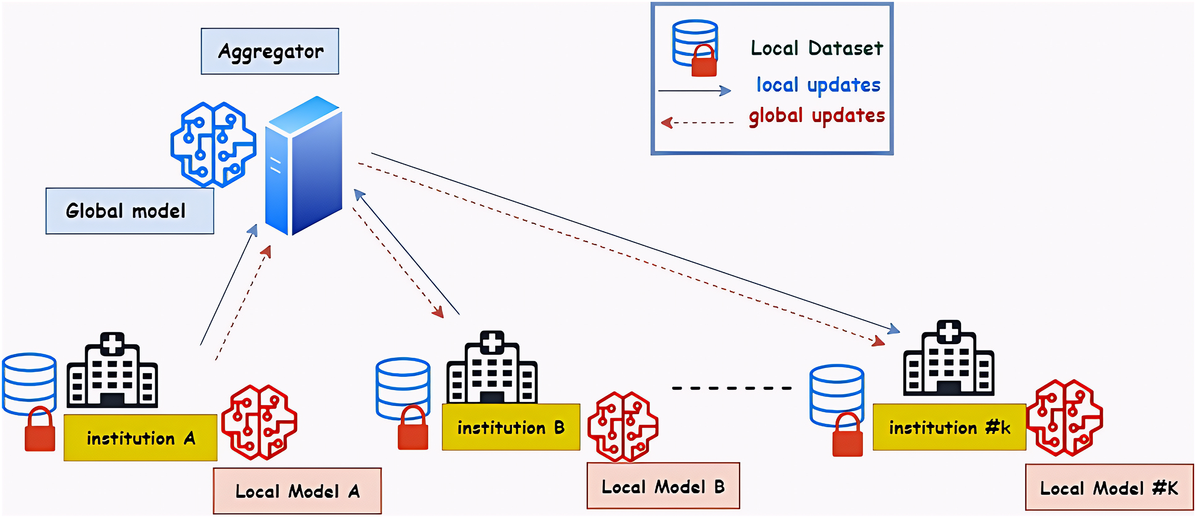
A federated machine learning system, which is regarded as a large-scale distributed system, is made up of numerous users and components, each of which has specific needs and limitations (Hua et al., 2019). Four key elements make up the general architecture of federated learning. The federated learning approach’s architecture is shown in Fig. 1. The local dataset is used to train the model, which then transmits the results to the central server. The server then transmits the results to the global model so that it can learn from them. The new results are then sent to every local model by the global model (Sherstinsky, 2020).

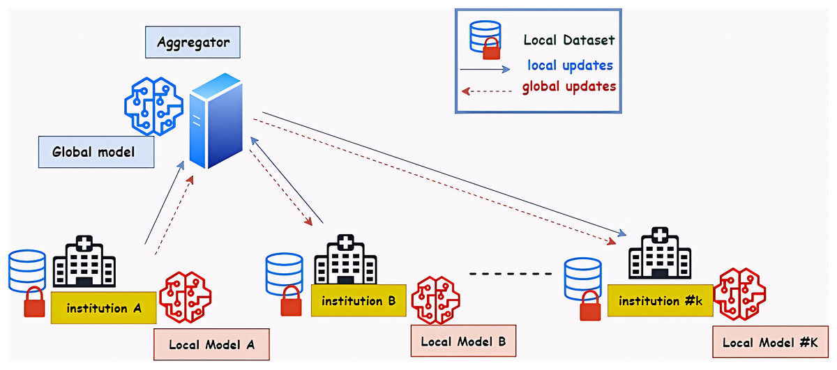
Figure 1: The architecture of the federated learning approach—hospitals represent the medical institution.

Download full-size image

DOI: 10.7717/peerj-cs.3545/fig-1

The FL-based system coordinates model training across multiple distributed client devices that rely on a central server to store data. Model training is done locally on the client device without moving data out of the client device. Federated learning can also be done in a distributed manner (Baid et al., 2021).

Swarm intelligence

Deep learning technology is one of the most popular and powerful methods of computer vision. While it has been quite successful, it is also like a black box method since it requires a lot of expertise in one particular domain as well as a lot of time spent tuning manually by trial and error. On the other hand, Swarm intelligence (SI) techniques are derivative-free and inspired by natural phenomena. It has the capability of solving complex optimization problems and can be integrated with DL to design efficient automated models and reduce human intervention. In this study, we applied two swarm intelligence algorithms Bayesian search optimization algorithm and sparrow search optimization algorithm (Bharti, Biswas & Shukla, 2023).

Bayesian search optimization algorithm

Bayesian search optimization algorithm (BOA) was selected for its ability to apply Bayesian statistics to the search for lost objects. BOA is a sequential model-based optimization that uses probabilities to solve statistical problems and can be mathematically expressed as Bayes’ rule of conditional probabilities. Based on a set of hyperparameter values, it computes the conditional probability of the objective function score (Pelikan, 2005).

The deep learning model is trained by selecting the hyperparameter values from the defined search space to predict the objective function. The model is evaluated for its prediction error and sent back to the optimizer for further iteration. Based on the results of previous iterations, it determines the next hyperparameters as it attempts to find the best value. The Bayesian algorithm has five aspects to be considered.

Search space: a defined set of values for each hyperparameter which to search for its appropriate value.
Objective function: A function that takes in hyperparameters and returns a score that would like to maximize or minimize.
Surrogate model: Analyzes previous evaluations to construct a probability representation of the objective function. Bayesian optimization use the Gaussian processes (GP) as the Surrogate model.
Acquisition functions: determine which hyperparameters in the search space to be chosen next from the surrogate model based on exploitation and exploration techniques. Exploitation means obtaining hyperparameters where a high objective is predicted by a surrogate model and exploration means obtaining hyperparameters at high-uncertainty locations.
Score history: history of the hyperparameters score to update the surrogate model.

The following pseudocode Algorithm 1 illustrates the steps of the Bayesian optimization algorithm.

Algorithm 1 :

Bayesian optimization algorithm.

1: Define search space for each hyperparameter X

2: Determine the objective function f needs to be maximized or minimized

3: initialize the surrogate model

4: while

(t < M a x i m u m i t e r a t i o n n u m b e r)

5: if

s u r r o g a t e m o d e l

is initialized then

u s e t h e s e t o f p o i n t s w i t h t h e l a r g e s t A C s e l e c t e d i n t h e p r e v i o u s i t e r a t i o n

A p p l y G a u s s i a n p r o c e s s e s

D e t e r m i n e t h e t y p e o f A c q u i s i t i o n f u n c t i o n

o b t a i n t h e p o i n t o f t h e l a r g e s t A c q u i s i t i o n f u n c t i o n s

10:

t + 1

11: else

12:

I n i t i a l i z e t h e s u r r o g a t e m o d e l a n d g o t o l i n e 4

13: end if

14: end while

DOI: 10.7717/peerj-cs.3545/table-15

Sparrow search algorithm

The Sparrow Search Algorithm (SSA) is one of the recent SI algorithms. This algorithm has the advantage of being accurate and efficient, as well as having a robust optimization feature that can be used to solve multiple optimization problems. The inspiration for this algorithm was taken from the concept of foraging as well as from the behavior of sparrow populations (Gharehchopogh et al., 2022).

In sparrow biology, there are two main groups characterized by significant characteristics. The first group is referred to as producers, while the second group is referred to as scroungers. The producers are those that locate food sources, while the scroungers are those who seek out food based on a guide given by the producer.

To prevent predator attacks during the foraging process, sparrows can be equipped with an efficient anti-prediction capability as scouters. Furthermore, producers and scavengers can alter their roles dynamically in order to obtain a good food source. Additionally, scroungers are capable of locating better food sources obtained by producers, whereas some scroungers are capable of locating the producer’s position so that they can obtain additional food (Xue & Shen, 2020). The equations that defined the SSA methodology can be verified as follow: At the first, the sparrows’ position is determined based on the following matrix dimensions.

(1) $X = [\begin{matrix} [\begin{matrix} X_{1, 1} & \dots & X_{1, d} \\ ⋮ & ⋱ & ⋮ \\ X_{n, 1} & \dots & X_{n, d} \end{matrix}] \end{matrix}] .$

As the d represents the dimensions and the n specifies the number of sparrows, these types of sparrows are considered producers if their energy levels are high. Foraging zones for scavengers are delivered to producers by their task of finding areas with rich food. As a result of the following matrix, the cost value of the sparrow can be determined: The scavengers begin to follow the producers until the producers find suitable food. There is a competition between scroungers for the food found by the producers. The scrounger who wins gets the food provided by the producers. The positions of the scroungers are updated by the following equation:

(2) $F_{X} = [\begin{matrix} f (X_{1, 1} & \dots & X_{1, d}) \\ ⋮ & ⋱ & ⋮ \\ f (X_{n, 1} & \dots & X_{n, d}) \end{matrix}] .$

When the sparrows are able to locate the predators, they will use their alarms to communicate with the other using a three-shielding criterion. When the alarm’s value is high enough in quantity to exceed the threshold of safety, the produced will be able to direct the scavenger to a safe location. The producers have the best cost values with a high chance of finding food compared to the scavengers. Based on the following equation, the position of the producers is updated:

(3) $X_{i, j}^{t + 1} = {\begin{matrix} X_{i, j}^{t} \exp (- \frac{i}{β \cdot i t e r_{m a x}}), & i f R_{2} \leq S T \\ X_{(i, j)}^{t} + Q * L, & i f R_{2} \geq S T \end{matrix}$ where $X_{i},_{j}^{t}$ the value of t is the current position of the producer for the jth dimension of the ith iteration t. $i t e r_{(m a x)}$ is considered to be the total iterations. ST represents the thresholding value within a range of [0.5, 1] while $R_{2}$ and $β$ represent a random value within a range of [0, 1] If $R_{2}$ is smaller than ST, the predator is not detected and the producer can search globally for food sources, whereas if R2 exceeds or equals ST, the producer can search for food sources globally. Sparrows detect predators, and as soon as they hear an alarm, the entire population flees for safety.

After the producers find good food, the scavengers begin to follow the producers. As the scavengers compete for the food found by the producers, the winner wins. The following equation is used to update the positions of scavengers:

(4) $X_{i, j}^{t + 1} = {\begin{matrix} Q \exp (\frac{X_{w o r e s t}^{t} - X_{p}^{t + 1}}{t^{2}}), & i f i \geq \frac{n}{2} \\ X_{p}^{t + 1} + ‖ X_{i, j}^{t} - X_{p}^{t + 1} ‖, X A^{+} & o t h e r w i s e \end{matrix} .$

As $X_{w o r s t}$ is the global worst population, and $X_{p}^{*}$ is the optimal position found by the producer, and $A^{+}$ is defined as

$A^{+} = A^{T} \cdot (A \cdot A^{T})^{- 1} .$

If $i > \frac{n}{2}$ : in the event of danger and the sparrows are aware of this, their positions are updated using the equation below. The scroungers leave their current position to search for food in other areas; otherwise, they will move toward producers and compete for food according to:

$X_{i}^{t + 1} = Q \exp (\frac{X_{w o r s t}^{t} - X_{p}^{t + 1}}{t^{2}}) i f i \geq \frac{n}{2} .$

(5) $X_{i, j}^{t + 1} = {\begin{matrix} X_{b e s t}^{t} + α ‖ X_{i, j}^{t} - X_{b e s t}^{t + 1} ‖ x, & i f f_{i} > f_{g} \\ X_{i, j}^{t} + K * (\frac{‖ X_{i, j}^{t} - X_{b e s t}^{t + 1} ‖}{(f_{i} - f_{φ}) + ε}) & f_{i} = f_{g} \end{matrix}$ where, $X_{b e s t}^{t}$ is known as the current global optimal location, $α$ is a value that is distributed normally with mean equal to 0 and variance equal to 1, and K is defined as a random value from −1 to $1, f_{i}, f_{g}, f_{φ}$ are the values of the cost of the current, global and worst fitness value. The Pseudocode of the SSA is shown in Algorithm 2.

Algorithm 2 :

Sparrow search algorithm (SSA).

while

(t < t_{m a x})

2: Rank the fitness values and find the current best and worst individuals

R_{2} = r a n d o m (1)

4: for i = 1: Number of producers do

update the sparrow’s location using Eq. (3)

6: end for

for i = (Number of producers + 1): n do

8: update the sparrow’s location using Eq. (4)

end for

10: for i = 1: Number of sparrows whose receive the danger do

update the sparrow’s location using Eq. (5)

12: end for

14: Get the current new location;

if the new location is better than the previous then update it;

16: end if

t = t + 1

18: end while

r e t u r n X_{b e s t}, f_{b e s t}

DOI: 10.7717/peerj-cs.3545/table-16

Proposed model

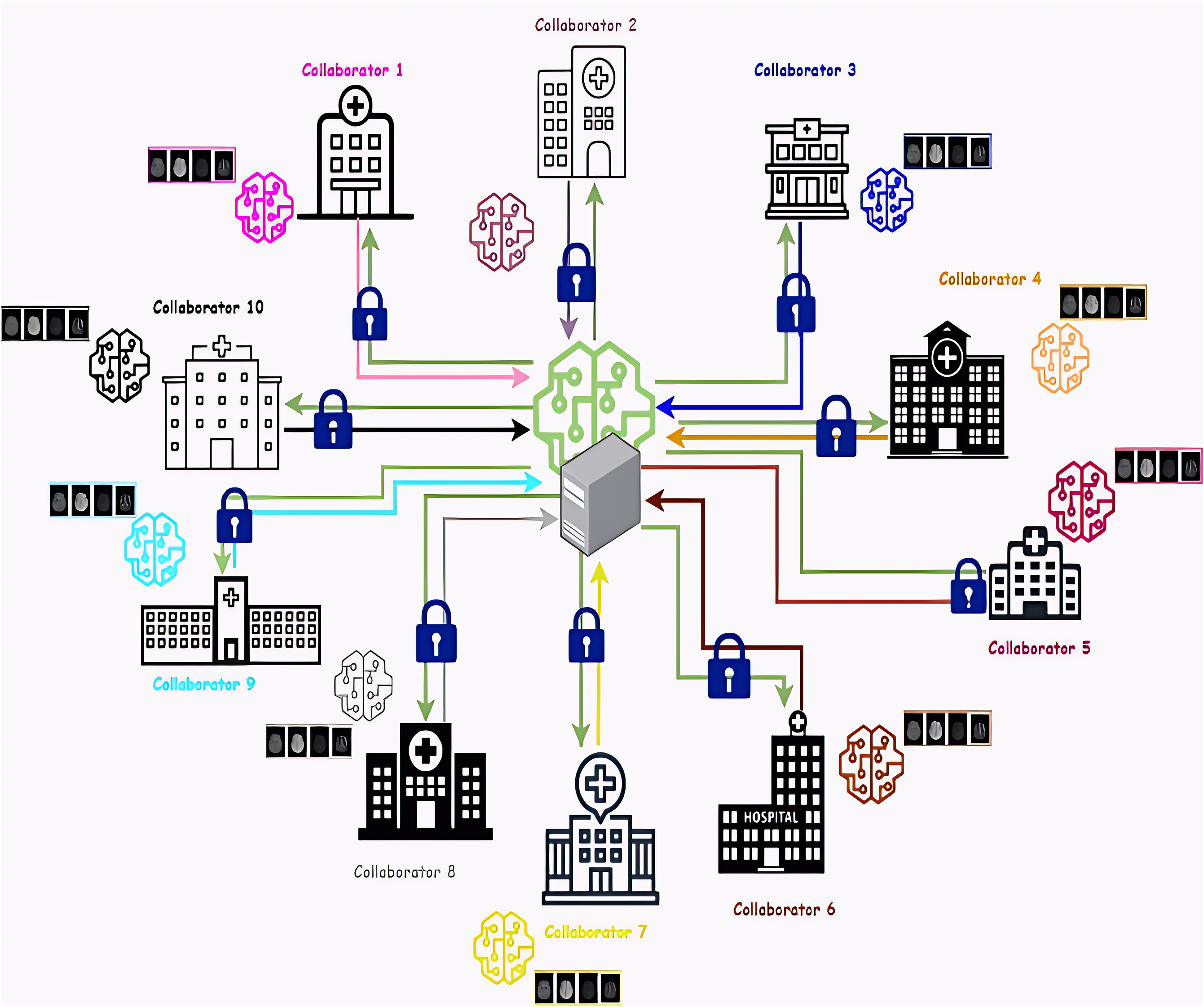
Federated learning is performed between two main components, the first component is the collaborators, which represent a bumper of medical institutions. The experiment was conducted with ten collaborators to simulate real life and address the challenges of many participating collaborators. Each collaborator trains a deep learning model locally using its private data without any data transfer. The second is the aggregator, a server responsible for aggregating the results of the local models from each collaborator and then sending these results to the global training model to learn from them. After that, it sends the global model’s resulting updates to the collaborators. Figure 2 represents the architecture of the proposed federated Learning system. we proposed a deep-learning training model based on a combination of convolution neural network (CNN) layers and recurrent neural network (RNN) layers to predict the MGMT gene value using different four Magnetic resonance imaging (MRI) scans (Fluid Attenuated Inversion Recovery (FLAIR), T1-weighted (T1w), T1-weighted Gadolinium Post Contrast (T1wCE/T1Gd), and T2-weighted (T2w)). Model hyperparameters are tuned using two search optimization algorithms: Bayesian Search (BO) and Sparrow Search optimization (SSA).

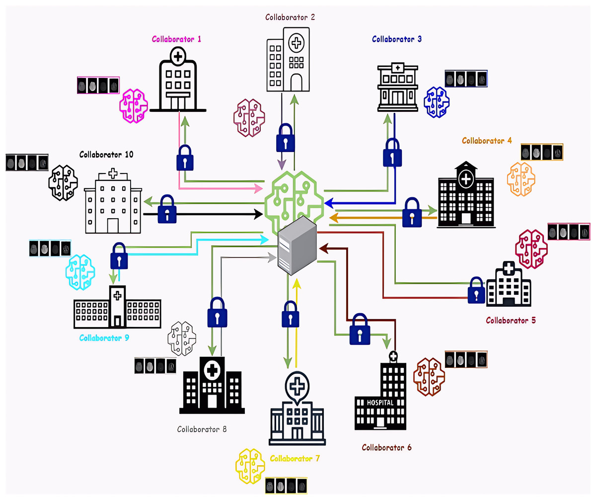
Figure 2: Architecture of the proposed federated learning system.

Download full-size image

DOI: 10.7717/peerj-cs.3545/fig-2

The ten collaborators are represented as different hospitals. The global model and the aggregator server are posed in the center, the green lines represent the provided updates from the global model to each local model and the colored lines represent the local model’s gradients that are sent to the global model. Network connections between the collaborators and the aggregator in federated learning are encrypted using Transport Layer Security (TLS).

BrainGeneDeepNet

BrainGeneDeepNet is based on convolution neural network architecture relying on RNN layers. The CNN architecture is composed of different repeated MBConv blocks and fully connected layers. An RNN architecture based on a long short-term memory (LSTM) layer receives features taken from the CNN architecture. A sequence input layer, two LSTM layers, two dropout layers, one fully connected layer, and a SoftMax layer receive the output of the completely connected layer.

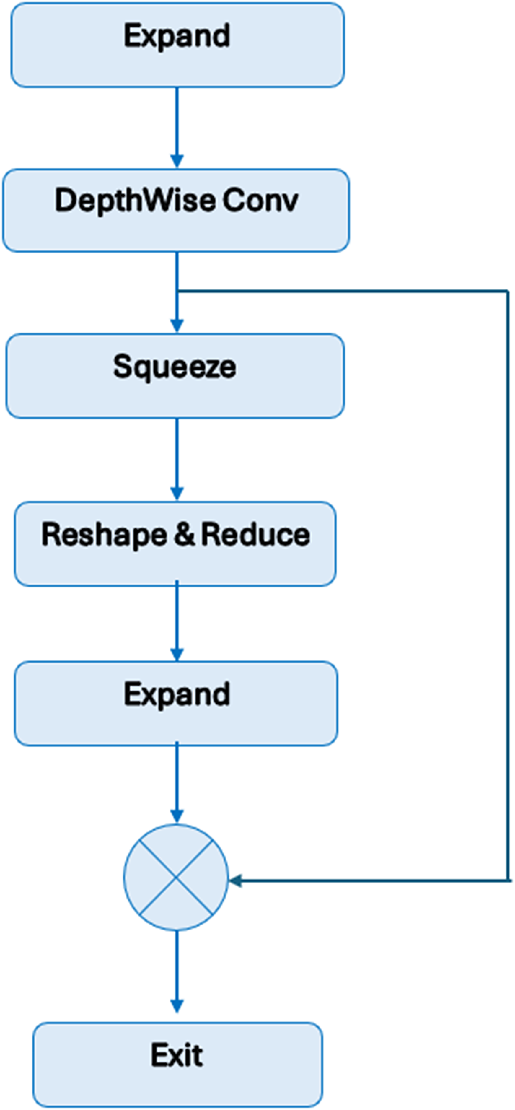
Figure 3 shows the MBConv block’s construction. Depthwise convolutions and a 1 × 1 projection layer come after the initial layer, which is a 1 × 1 expansion convolution. A residual link is made between the input and the output if their channel numbers match.

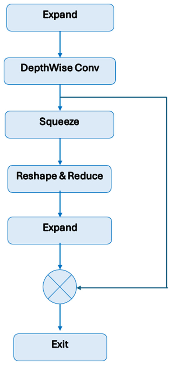
Figure 3: Structure of MBConv block.

Download full-size image

DOI: 10.7717/peerj-cs.3545/fig-3

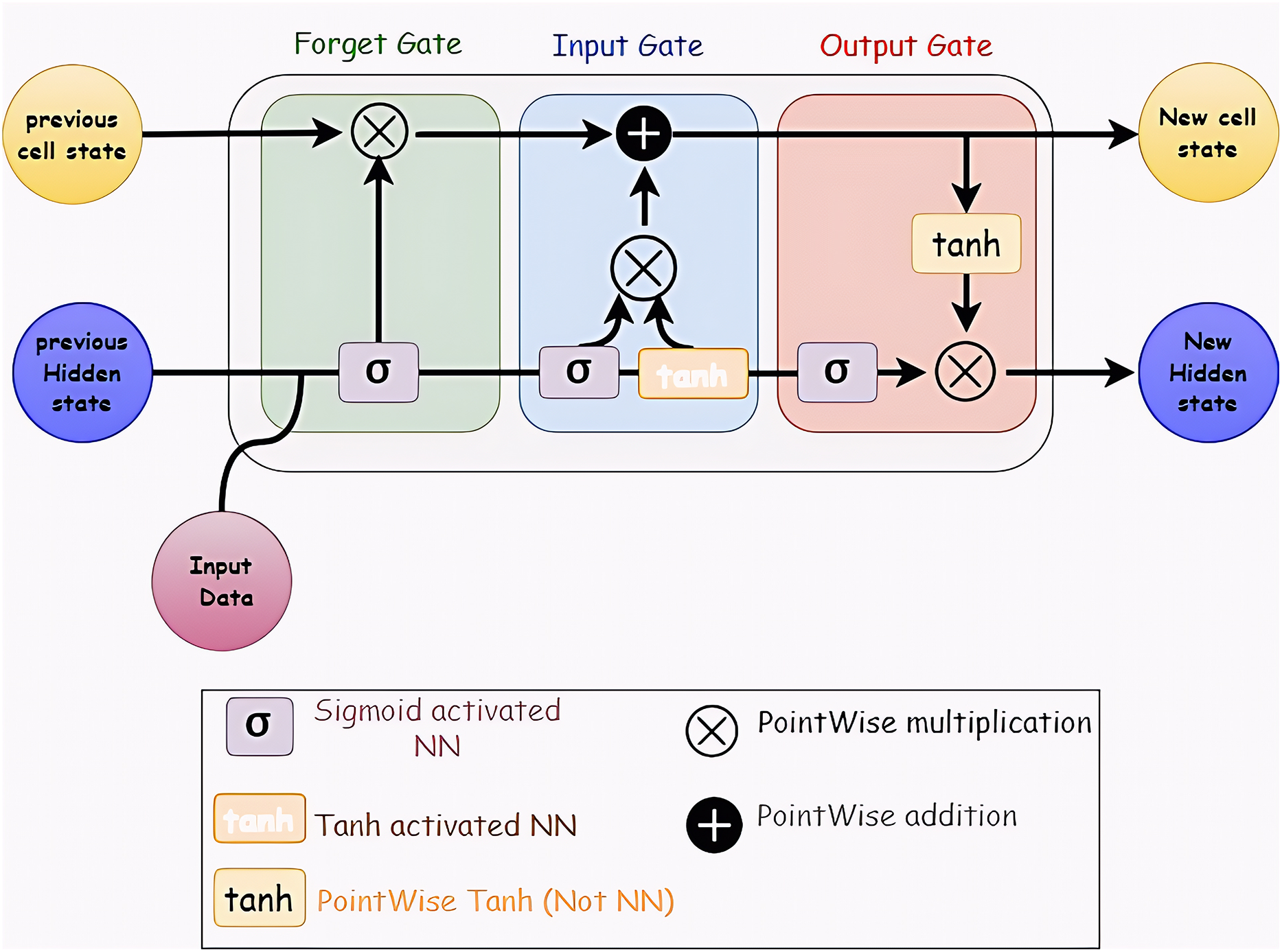
Long Short-Term Memory (LSTM) networks in recurrent neural networks can learn order dependency from the results of earlier stages. Because the output from the previous phase is used as an input in the next step, RNNs are appropriate for time series data processing, prediction, and classification (Hua et al., 2019; Sherstinsky, 2020). Figure 4 shows the LSTM layer’s structure.

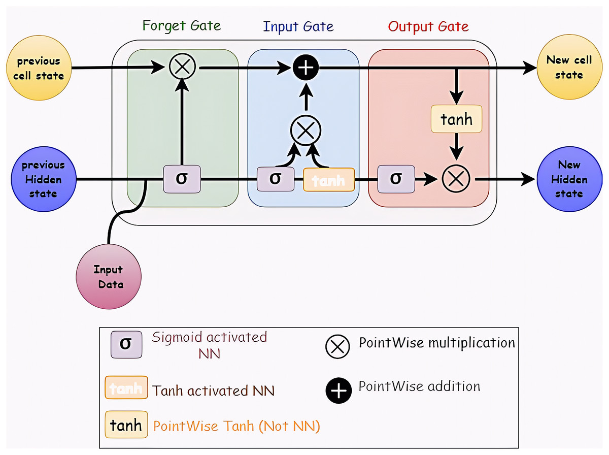
Figure 4: Structure of LSTM network.

Download full-size image

DOI: 10.7717/peerj-cs.3545/fig-4

It consists of many memory units called cells arranged in a chain topology and four neural networks. Three gates—an input gate, an output gate, and a forget gate—control the flow of data into and out of the cell.

Figure 5 shows BrainGeneDeepNet’s complete neural network design. The kernel size is defined by K3 × 3/k5 × 5, the fully connected layer is denoted by FC, the tensor shape (height, width, and depth) is represented by H × W × F, and the multiplier for multiple repeated layers is ×1/2/3/4.

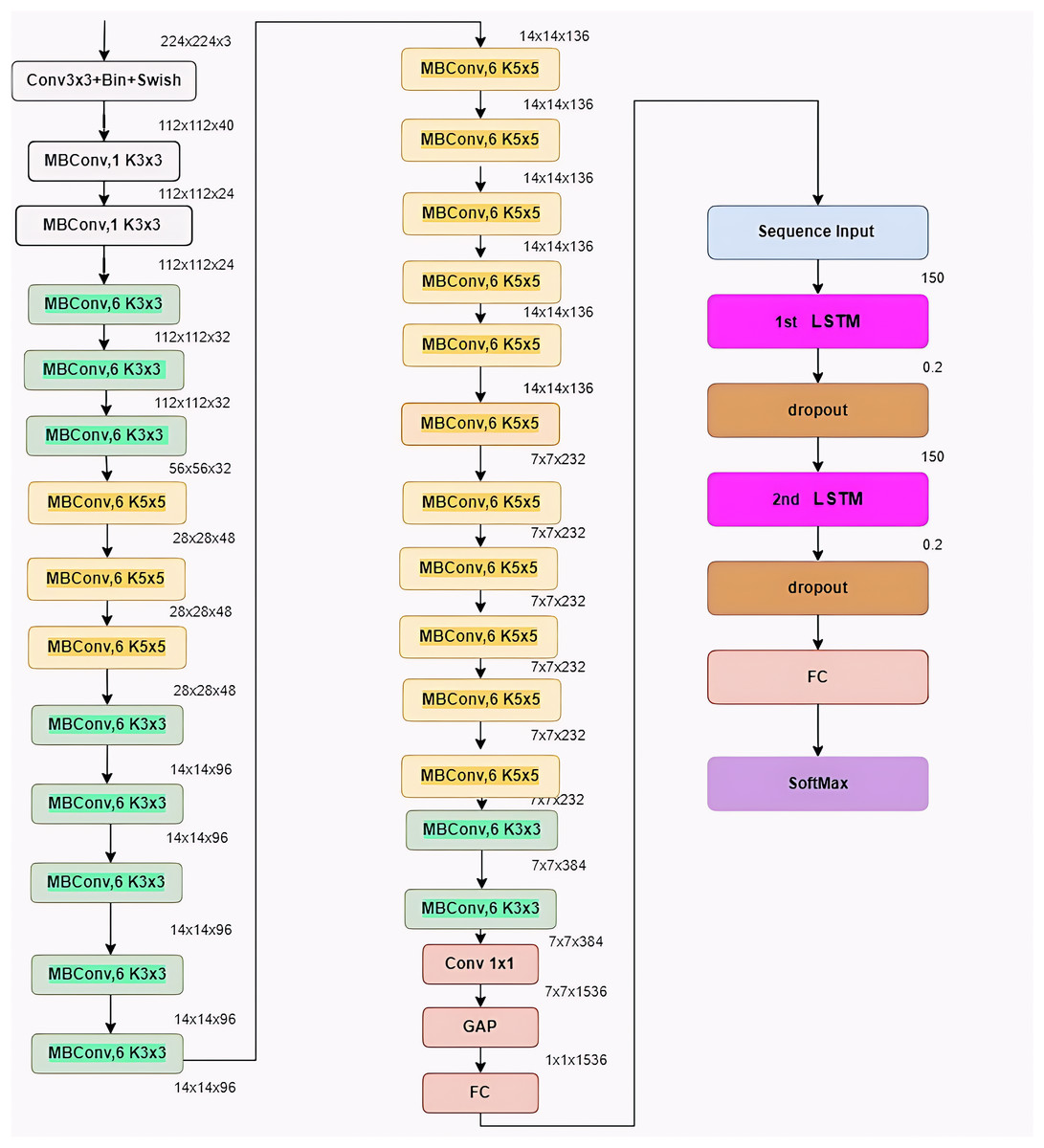
Figure 5: Architecture of the proposed model.

Download full-size image

DOI: 10.7717/peerj-cs.3545/fig-5

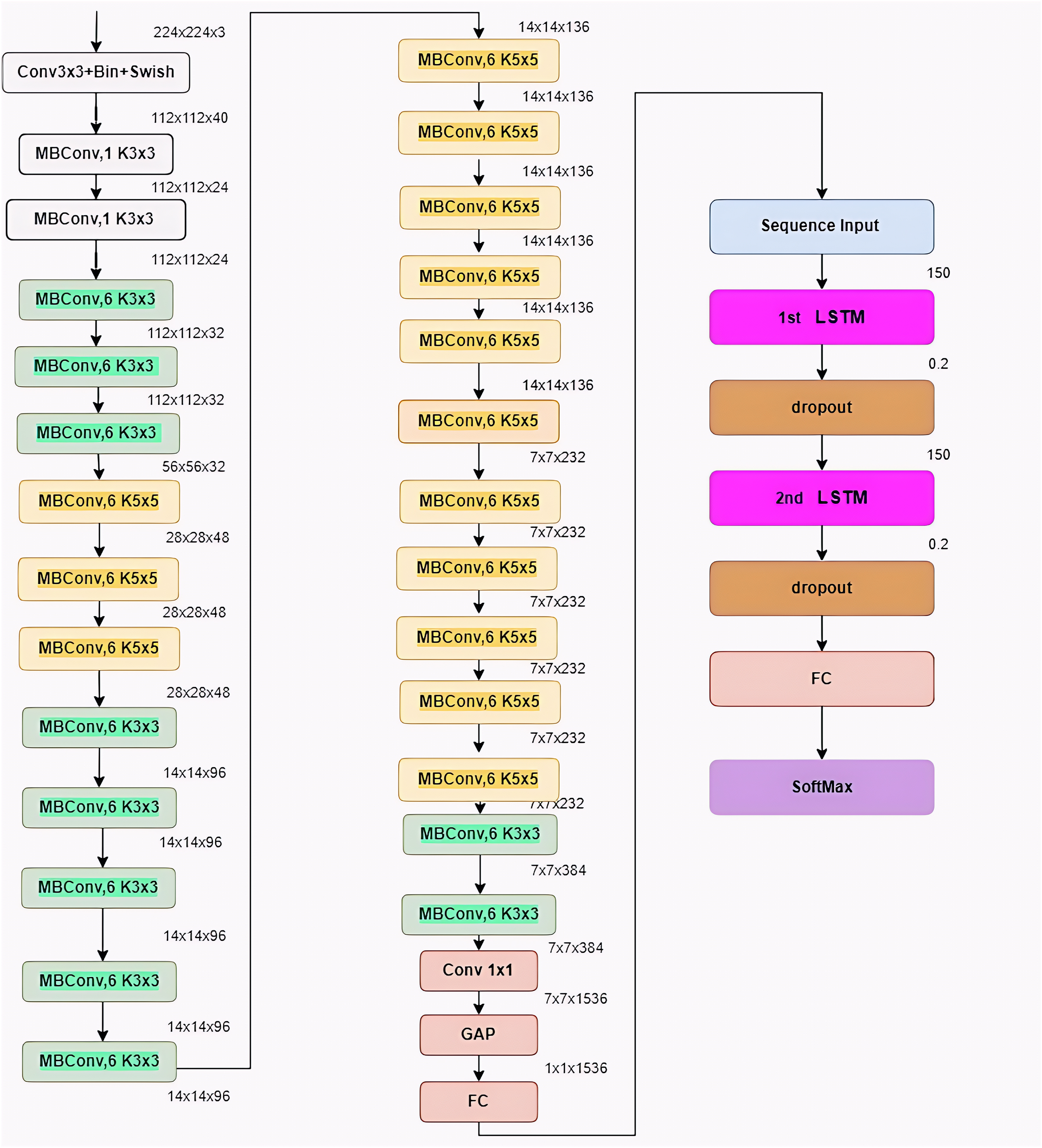
To attain high-accuracy performance, the architecture is modified in a number of ways. The optimizer, which is the first parameter, is chosen to be adaptive moment estimation (Adam). The learning rate, which is the second parameter, is set at 0.001. While the number of iterations for each epoch is equal to 58, the third parameter, the number of model epochs, is defined as 20. Batch normalization and a 40% dropout are used before each fully linked layer to avoid overfitting. The two-class classification problem is solved on the last layer using a sigmoid activation function. The two-class classification problem is solved by using a binary cross-entropy function for the cost function. Additionally, the RNN architecture has certain settings changed. Each LSTM layer includes 150 neurons, and the probability value of the dropout layer is 0.2.

Using different scan types can be considered a contribution that emphasizes the accuracy of the results. So, the proposed model is trained with the four sequence types of MRI scans. Several experiments are conducted to achieve the best accuracy. Experiments 1, 2, 3 and 4 were conducted with FLAIR, T1w, T1wCE and T2w respectively. Experiment 5 with a combination of two types of scans which are T1w and T2w scans, Experiment 6 with a combination of three types of scans which are T1w, T2w, and FLAIR and finally, Experiment 7 conducted with a combination of the four types of scans.

Different models based on the scan types FLAIR, T1w, T1wCE, T2w, and a combination of two or more scans are used for the training process. Every model determines the likelihood that it falls into class 0 (no MGMT) or class 1 (present MGMT). The calculation of MGMT value differs in each experiment based on the used sequence type. Experiments 1, 2, 3 and 4 were conducted with one sequence type, so the resulting value is the MGMT value. In Experiments 5 and 6 the final score of MGMT value is the mean of the resulting value of each scan. In the last experiment, The variance between the mean and the minimum as well as the difference between the mean and the maximum are utilized to compute the MGMT value for the four sequence types.

Algorithm 3 illustrates how each patient’s final score is determined. Each scan type contains the identical pre-processing and training processes, even though the training model operates on them independently. The MGMT value of each patient is ultimately predicted by adding up all of the forecasts that were made. To choose the most confident outcome among all forecasts, the prediction results are combined for every patient. The mean of each patient’s four different scan types is obtained in order to apply the aggregation method. Additionally, the minimum and maximum are computed. The variance between the mean and the minimum as well as the difference between the mean and the maximum are then compared. Lastly, the ideal value (maximum or minimum) is the difference that is closest to the mean.

Algorithm 3 :

Predicting MGMT value.

1: Predicted MGMT Value: List

2: for each scan type [‘flair’, ‘t1w’, ‘t1wce’, ‘t2w’] do:

T r a i n_d f, V a l d_d f \Leftarrow c r e a t e a d a t a f r a m e f o r t h e t r a i n i n g a n d v a l i d a t i o n s e t s

T e s t_d f \Leftarrow c r e a t e a d a t a f r a m e f o r t h e t e s t i n g s e t

T r a i n_g, V a l d_g, T e s t_g \Leftarrow D a t a_A g u m e n t a t i o n (T r a i n_d f, V a l d_d f, T e s t_d f)

b e s t M o d e l \Leftarrow t r a i n i n g M o d e l (M R I S c a n T y p e, T r a i n_g, V a l d_g, E = 20)

T e s t P r e d \Leftarrow b e s t M o d e l . p r e d i c t i o n (T e s t_g)

T e s t_d f [P r e d_y] \Leftarrow T e s t_p r e d

M e a n P r e d \Leftarrow T e s t P r e d . m e a n ()

10:

T e s t P r e d A g g \Leftarrow A g g r e g a t e r e s u l t s o n a l l M R I t y p e s f o r e a c h p a t i e n t

11: for each patient id do:

12: if Max

(T e s t_d f [P r e d_y]) - M e a n P r e d > M e a n P r e d - M i n (T e s t_d f [P r e d_y])

then

13:

T e s t P r e d A g g \leftarrow max (T e s t_d f [P r e d_y])

14: else

15:

M i n (T e s t_d f [P r e d_y])

16: end if

17: end for

18: end for

DOI: 10.7717/peerj-cs.3545/table-17

Step 1: A validation set is created from 10% of the training data. The main reason for this is to validate the performance of the training model. In addition to this, three data frames are designed for the training, validation, and test data so that they can be ready for further steps.

Step 2: The photos undergo data augmentation, and the kind of augmentation used was based on geometric methods. Prior to training, the augmentation stage seeks to balance the quantity of images in each class. As a result, some procedures are carried out on pictures with various values. as illustrated in Table 2.

Table 2:

Agumentation values.

Operations	Parameter’s value
Rescale	1.0/255
Zoom	Range: 0.2
Rotation	Range: 0.2
Fill	Mode = ‘nearest’
Height shift	Range = 0.1
Width shift	Range = 0.1
Horizontal flip	True
Brightness	Range = [0.8, 1.2]

DOI: 10.7717/peerj-cs.3545/table-2

It is also important to note that the former operations are applied to the training data, while the validation and testing data have the rescale operation only being applied to obtain augmented train, validation, and test data frames.

Step 3: The entire set of original and modified training and validation data is fed into the BrainGeneDeepNet model. A few parameters pertaining to the number of epochs and iterations are used to train the model. The model’s epochs are defined with 20, and each epoch has 58 iterations. This results in 1,160 iterations for the full model. Step 4: when the training on the validation and training data is finished. The trained model can now be used to verify the test data. To choose the most confident outcome among all forecasts, the prediction results are combined for each patient. The mean of each patient’s four scan types is obtained in order to apply the aggregation method. Additionally, calculations are made for the maximum and minimum. Next, a comparison is made between the variance between the mean and the minimum and the difference between the mean and the maximum. Lastly, the ideal value (maximum or minimum) is the one that deviates from the mean the least.

Bayesian-based model

Despite the efficiency of the proposed model, it consumed hundreds of communication rounds between the participant’s collaborators to achieve the desired accuracy. The model’s performance was improved using two swarm intelligence techniques to achieve higher accuracy with fewer communication rounds. The first algorithm was the Bayesian optimization algorithm (BO). BO is a sequential model-based optimization that uses probabilities to solve statistical problems and can be mathematically expressed as Bayes’ rule of conditional probabilities. The following algorithm (Algorithm 4) shows how the BO algorithm was applied to optimize the performance of the proposed model.

Algorithm 4 :

Bayesian-based model.

F l R o u n d \Leftarrow [80 : 150]

E p o c h e s \Leftarrow [30 : 100]

L e a r n i n g R a t e \Leftarrow [0.01 : 1]

M a x A c c \Leftarrow C u r r e n t M o d e l T e s t A c c

M i n F l R \Leftarrow C u r r e n t M o d e l F l R o u n d s

T a r g e t F \Leftarrow M a x A c c w i t h M i n F l R o u n d

t r a i n B r a i n G e n e D e e p N e t (M R I_S c a n_t y p e, T r a i n_g, V a l d_g, E p o c h s)

t = 1

9: while

t < G

do:

10:

B e s t P o i n t s \Leftarrow A c q u i s i t i o n f u n c t i o n s t o c h o o s e t h e b e s t p o i n t o f f u n c t i o n f

11:

S a m p l e P o i n t s \Leftarrow A c q u i r i n g s a m p l i n g p o i n t s f r o m t h e a c q u i s i t i o n f u n c t i o n

12:

V a l i d a t i o n S e t \Leftarrow T a r g e t F (S a m p l e P o i n t s)

13:

A n a l y z i n g t h e s t a t i s t i c a l G a u s s i a n d i s t r i b u t i o n m o d e l a n d u p d a t i n g i t

14: if

C u r r e n t M o d e l T e s t A c c > M a x A c c \land M o d e l F L R o u n d s < M i n F L R

then

15:

M a x A c c \Leftarrow C u r r e n t M o d e l T e s t A c c

16:

M i n F L R \Leftarrow C u r r e n t M o d e l F L R o u n d s

17: end if

18:

go t o s t e p 10

19:

t = t + 1

20: end while

21:

R e t u r n X_{1, 2, 3 \dots b e s t}, f_{b e s t}

DOI: 10.7717/peerj-cs.3545/table-18

Step 1: Define the search space for each hyperparameter

Step 2: Using the training and validation data as inputs, create the objective function for the Bayesian optimizer.

Step 3: choose the best point of function f using the Acquisition functions

Step 4: Acquiring sampling points from the acquisition function.

Step 5: apply the objective function with the acquired samples and obtain results in the validation set.

Step 6: update the statistical Gaussian distribution model.

Step 7: check if the terminated conditions is satisfied.

Sparrow-based model

A sparrow-based model mimics the behavior of a sparrow as a swarm. The core idea is that swarm members follow the group leader to get food or catch prey. The following algorithm shows how the SSA algorithm was applied to optimize the performance of the proposed model. After determining the initial structure of the proposed model and all the relevant parameters of the MGMT algorithm.

Algorithm 5 shows the structure of the sparrow search algorithm.

Algorithm 5 :

Sparrow-based model.

N = 100, G = 20, S D = 50, P D = 50, t = 1

t r a i n_{B} r a i n G e n e D e e p N e t (M R I S c a n t y p e, T r a i n_{g}, V a l d_{g}, E p o c h s = 20)

M a x A c c \Leftarrow C u r r e n t M o d e l T e s t A c c

M i n F l R \Leftarrow C u r r e n t M o d e l F l R o u n d s

5: while

t < G

do:

F i n d t h e p o s i t i o n o f t h e b e s t a n d w o r s t s p a r r o w a c c o r d i n g t o f i t n e s s v a l u e s

R \Leftarrow G e n e r a t e r a n d o m n u m b e r

8: for i = 1: PD do:

U p d a t e t h e l o c a t i o n o f t h e d i s c o v e r e r s

10: end for

11:

R \Leftarrow U p d a t e t h e w o r s t l o c a t i o n f o u n d b y t h e d i s c o v e r e r

12: for i = (PD + 1): N do:

13:

U p d a t e t h e l o c a t i o n o f t h e f o l l o w e r s

14: end for

15: for i = 1: SD do:

16:

G e t t h e i n d i v i d u a l p o s i t i o n o f a s p a r r o w t h a t i s a w a r e o f d a n g e r

17: end for

18: if

C u r r e n t M o d e l T e s t A c c > M a x A c c \land M o d e l F L R o u n d s < M i n F L R

then

19:

M a x A c c \Leftarrow C u r r e n t M o d e l T e s t A c c

20:

M i n F L R \Leftarrow C u r r e n t M o d e l F L R o u n d s

21: end if

22:

g o t o s t e p 6

23:

t = t + 1

24: endwhile

25:

R e t u r n X_b e s t, f_b e s t

DOI: 10.7717/peerj-cs.3545/table-19

Evaluation method

To evaluate the effectiveness of the proposed BrainGeneDeepNet model, several validation procedures were employed. First, a hold-out validation strategy was applied by reserving 10% of the training data for validation. In the federated learning setup, each participating institution also maintained its own local validation set, corresponding to 10% of its training data. Second, comparative experiments were conducted against seven widely used neural network architectures (AlexNet, VGG16, ResNet18, ResNet34, ResNet50, InceptionV3, and EfficientNetB3), all trained under identical settings, to assess the relative performance of the proposed model. Third, ablation studies were performed using individual MRI modalities (FLAIR, T1W, T1WcE, and T2W) as well as their combinations in order to quantify the contribution of each modality to predictive performance. In addition, the proposed federated learning approach was evaluated against the classical centralized training approach to demonstrate the benefits of the federated setup in terms of accuracy, privacy, and robustness. Finally, hyperparameter optimization using Bayesian Optimization and Sparrow Search Optimization algorithms was applied, and their impact on model performance was validated empirically.

Evaluation metrics

To evaluate the performance of the proposed model, we used several commonly adopted metrics in medical image analysis, namely Accuracy, Loss, AUC, Recall, and Precision. Their mathematical definitions are presented below.

Accuracy: Accuracy measures the proportion of correctly classified cases out of the total samples:

(6) $A c c u r a c y = \frac{T P + T N}{T P + T N + F P + F N} .$ Loss: We used the binary cross-entropy loss function:

(7) $L o s s = - \frac{1}{N} \sum_{i = 1}^{N} [y_{i} \log ({\hat{y}}_{i}) + (1 - y_{i}) \log (1 - {\hat{y}}_{i})]$ where $y_{i}$ is the ground truth label and ${\hat{y}}_{i}$ is the predicted probability.

Area Under the ROC Curve (AUC): AUC evaluates the separability of classes by integrating the True Positive Rate (TPR) against the False Positive Rate (FPR):

(8) $A U C = \int_{0}^{1} T P R (F P R) d (F P R) .$ Recall (Sensitivity) Recall quantifies the ability to correctly identify positive cases:

(9) $R e c a l l = \frac{T P}{T P + F N} .$ Precision: Precision measures the proportion of correctly identified positives among all predicted positives:

(10) $P r e c i s i o n = \frac{T P}{T P + F P} .$ where TP, TN, FP, and FN denote true positives, true negatives, false positives, and false negatives, respectively.

Experimental setup

BRATS2021 dataset

The Radiological Society of North America (RSNA) has contributed a large collection of MRI images in partnership with the Medical Image Computing and Computer-Assisted Intervention Society (the MICCAI Society).The dataset is accessible to the general public at https://www.kaggle.com/datasets/dschettler8845/brats-2021-task1. There are many different types of brain tumors in this dataset. The multiparametric magnetic resonance imaging (mpMRI) scans were obtained under standard clinical conditions at a number of different institutions using various imaging equipment and protocols. As a result, the image quality was largely heterogeneous, reflecting the variations in clinical practice among the institutions under study (Baid et al., 2021).

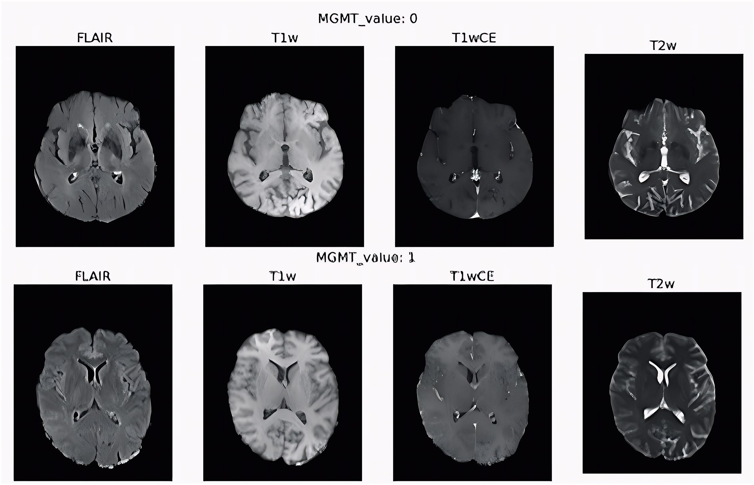
Each patient has a separate collection of images from four different types of scans Fluid Attenuated Inversion Recovery (FLAIR), T1-weighted (T1w), T1-weighted Gadolinium Post Contrast (T1wCE/T1Gd), and T2-weighted (T2w) visualizing the anatomy in three planes. The first one is from front to back (coronal plane), the second from top to down (axial plane), and the third side to side (sagittal plane). Additionally, the plans of the four types of MRI sequences for the same patient are not the same. The training set consists of the scans of 585 patients, while the testing set consists of 87 scans.

They defined the MGMT promoter methylation status for all the patients as a binary label, 1 for the methylated case and 0 for unmethylated. The four types of scans for two patients with different MGMT values are shown in Fig. 6. The first row is the scans of the patient with 0 value for MGMT gene and the second row for patient with 1 value for MGMT gene. The chemotherapy medication is predicted to be less effective the more MGMT protein the tumor produces because the protein will heal the damage to the tumor.

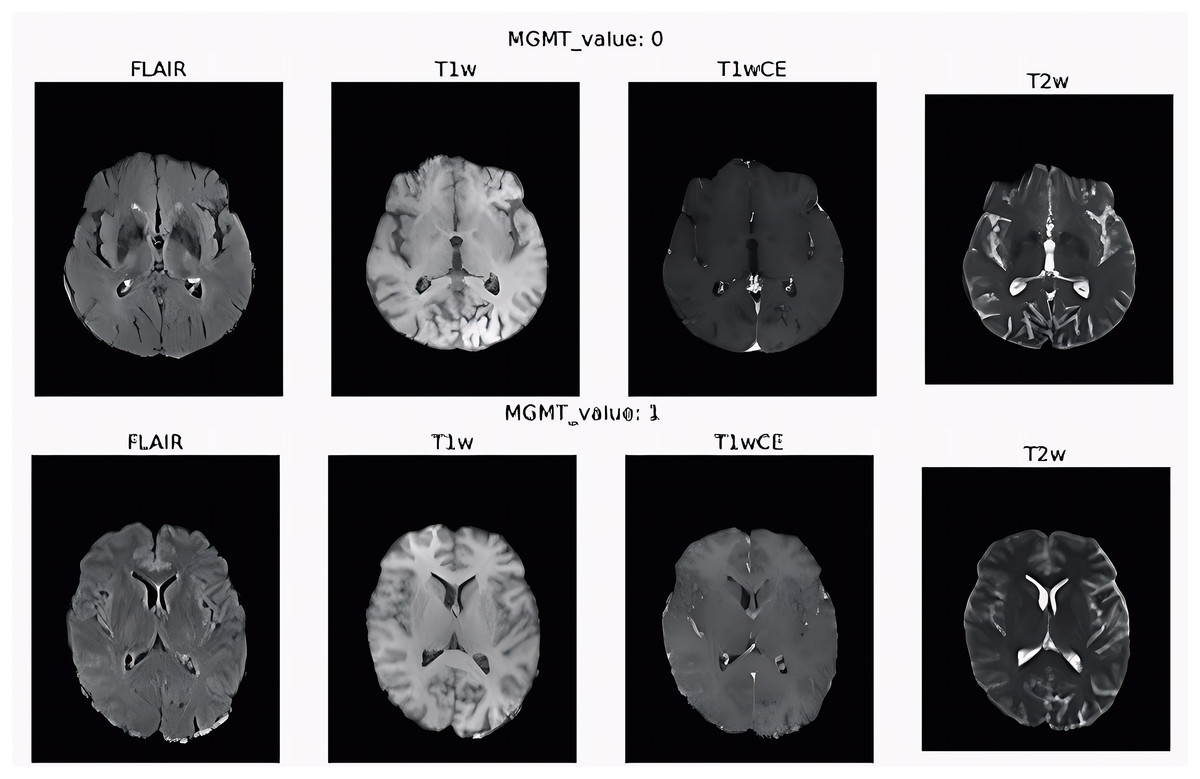
Figure 6: Four sequence scan types for two patients with different MGMT values.

Download full-size image

DOI: 10.7717/peerj-cs.3545/fig-6

Experimental scenarios

The federated experiments were conducted using the OpenFL framework across ten collaborators (institutions). Each collaborator trained models locally and shared only encrypted gradients with the central aggregator.

All experiments were conducted on a computing cluster where each node was equipped with an Intel Core i7 CPU, 32 GB of RAM, and a single NVIDIA GeForce RTX 3080 GPU (10 GB VRAM). The software environment was Python 3.8, PyTorch 1.11.0, and the OpenFL 1.3 framework. To comprehensively evaluate the proposed model, we conducted a series of experiments designed to assess different aspects of its performance. The experiments are organized as follows:

Scenarios 1 to 4 (Single Modality Performance): These experiments evaluated the performance of BrainGeneDeepNet and baseline models using each of the four MRI sequences individually: FLAIR (Exp. 1), T1w (Exp. 2), T1wCE (Exp. 3), and T2w (Exp. 4).
Scenarios 5 to 7 (Multi-Modality Fusion): These experiments investigated the impact of combining multiple MRI sequences: T1w + T2w (Exp. 5), T1w + T2w + FLAIR (Exp. 6), and all four sequences (Exp. 7).
Scenario 8 (Classical vs. Federated Learning): This experiment compared the performance of the best-performing model from the classical (centralized) setting against its federated learning counterpart.
Scenario 9 (Hyperparameter Optimization): This experiment applied the Bayesian Search (BO) and Sparrow Search (SSA) optimization algorithms to the federated model to enhance accuracy and reduce communication rounds.

This structured approach allows for a systematic analysis of modality contribution, the benefit of federated learning, and the efficacy of automated hyperparameter tuning.

During the data processing process, the DICOM sequences were converted into NIFTI (The Neuroimaging Informatics Technology Initiative) files. The NIFTI format is an improved version of the Analyze file format, designed to be simpler than DICOM while retaining all of the important metadata. We used a Python library called Dicom2nifti to make this conversion. Additionally, it has the advantage of storing volumes in a single file, with a simple header followed by raw data. As a result, a single NIfTi file can be handled rather than several hundreds of DICOM files.

The provided dataset host has notified that there are some issues in the training dataset with these three cases, the FLAIR sequences of the two patients with ID 00109 and 00709 are blank, and the TW1 sequence for the patient with ID 00123 is blank. So, the actual number of patient’s cases that is valid to train is 582.

We distributed the data from the two training and testing datasets among ten collaborators in order to replicate the actual setup of ten institutions. The resulting patient counts for each of the institutions—which we will call collaborators (C) 1–10—are provided at random with significant fluctuations, such as 80, 70, 75, 60, 35, 65, 50, 40, 36, and 70 patients respectively for the training set and given as 10, 9, 9, 8, 8, 8, 9, 8, 8, and 10 patients respectively for the testing set. Furthermore, for each institution, we hold out 10% of their training data as a validation set, i.e., local validation set.

The data was divided into several distinct datasets using the horizontal partitioning (sharding) technique. Despite having completely different patients, each segment shares the same qualities.

BrainGeneDeepNet

The BrainGeneDeepNet training process’s parameters are stated to particular values. Table 3 illustrates the stated values for the initial learning rate, number of epochs, number of iterations, learning rate optimizer and the classifier.

Table 3:

Training process parameters.

Parameter	Value
Learning rate	0.01
Number of epochs	20
Number of iterations	58
Optimizer	Adam
Classifier	SoftMax

DOI: 10.7717/peerj-cs.3545/table-3

To implement the BrainGeneDeepNet model in a federated environment we used the OpenFL framework (Reina et al., 2021) among ten collaborators. At first, the communication between the collaborators continued for 300 communication rounds to achieve the same accuracy as the classical method. To optimize the number of communication rounds and maximize the predictive accuracy we used two swarm intelligence algorithms, the Bayesian search optimization algorithm and the sparrow search optimization algorithm. Each optimization algorithm tuned the model’s parameters for 20 iterations. Table 4 illustrates the search space of each hyperparameter that the Bayesian algorithm will search for the best values between them.

Table 4:

Bayesian search algorithm parameters values.

Parameter	Search space
Learning rate	(0.01, 1)
Number of epochs	(30, 100)
Number of communication rounds	(80, 150)
Target function	Maximize training accuracy and minimize the number of communication round
Classifier	SoftMax

DOI: 10.7717/peerj-cs.3545/table-4

The results of the Bayesian algorithm showed that after 20 iterations, the algorithm was able to find the optimal parameters in iteration 17 that achieved the highest accuracy score of 97.22% when the initial learning rate is 0.07846386771844214 and 56 epochs through 113 communication rounds.

In order to ensure the validity of the model, the Sparrow Search optimization algorithm (SSA) is also utilized. Table 5 illustrates the initialization value for the parameters associated with the SSA. R is a random number generated in the boundaries of [−512, 512]. The total number of the sparrows is initialized as 100 and is divided into 50 producer sparrows and 50 Scroungers sparrows.

Table 5:

SSA parameters values.

Parameter	Search space
Population size	100
Producers	50
Scroungers	50
Iterations	20
R	Random value
Lower boundary	−512
Upper boundary	512
Dimensions	3
Objective function	Maximize training accuracy and minimize the number of communication rounds

DOI: 10.7717/peerj-cs.3545/table-5

The best accuracy was achieved in iteration 14, which is 0.97631, and the number of communication rounds is 91 while the learning rate is 0.035246840775015. The number of epochs is 99.

Results and discussion

As part of the evaluation of the proposed model, seven experiments have been conducted using the four sequence scan types FLAIR, T1W, T1WcE, T2W and several combinations of these scan types together as an input. In addition, comparing the proposed model against seven popular neural network architectures, including AlexNet (Krizhevsky, Sutskever & Hinton, 2017), Vgg16 (Simonyan & Zisserman, 2014), ResNet18, ResNet34, ResNet50 (He et al., 2015), InceptionV3 (Szegedy et al., 2015), and EfficientNetB3 (Tan & Le, 2019). It was found that BrainGeneDeepNet performed the best in terms of accuracy, loss, AUC, recall, and precision performance matrices.

In order to determine the best neural network architecture, the proposed model and the seven neural network architectures were trained with the same hyperparameters and prediction method. Among single MRI modalities, four experiments were conducted on the four sequence scan types individually (FLAIR, T1W, T1WcE and T2W). The T2w based on the proposed model achieved the highest accuracy value (94%). On the other hand, the T1WcE achieved the lowest accuracy value (89.2%). Among Multiple MRI modalities, three experiments were conducted with a combination of Sequence scan types (T1w + T2W, T1w + T2W + FLAIR, T1w + T2W + FLAIR + T1WcE), respectively. The combination of the four sequence types achieved the highest accuracy value (96%). The BrainGeneDeepNet was the most successful, however, it is based on classical learning techniques. Therefore, the BrainGeneDeepNet is developed in a federated environment to overcome the drawbacks of the classical approach, such as data privacy, centralizing computation, and high computational power. The BrainGeneDeepNet is developed in a federated environment with ten institutions involved in the federation. The Sparrow Search Optimization Algorithm (SSA) and Bayesian search optimization algorithm are used to select optimal training hyperparameters, such as the initial learning rate, the number of epochs, and the number of communication rounds, to maximize the predictive accuracy of the federated model.

The FL model and the classical model were tested on 87 patients and the MGMT values of these patients were obtained. Through the 91 communication rounds, the FL model achieved greater accuracy, AUC, recall, and precision, while resulting in fewer losses, demonstrating its efficiency over the classical model. Our FL experiment shows that, even with imbalanced and heterogeneous datasets, such as BraTS2021. The training model was 99.99% of the model quality attained with centralized data using the FL technique across ten universities. In addition to providing useful solutions for high processing power, centralized calculation, and data privacy.

The following tables and charts represent all the conducted experiment results in detail. Tables 6 to 10 describe experiments based on single MRI modalities. In contrast, Tables 11 and 12 describe experiments based on multiple MRI modalities. Table 13 illustrates the performance of BrainGeneDeepNet using single and multiple MRI modalities. In Table 14, a comparison between the classical and federated learning approaches is shown.

Table 6:

Experiment one results.

Performance	BrainGene	AlexNet	VGG16	ResNet-18	ResNet-34	ResNet-50	inceptionV3	EfficientB3
Accuracy	0.9125	0.7750	0.8252	0.7854	0.8229	0.8451	0.8580	0.8914
Loss	0.2551	0.6246	0.4974	0.7190	0.6069	0.5603	0.3663	0.3222
AUC	0.9516	0.8522	0.9212	0.8576	0.8989	0.9235	0.9379	0.9609
Recall	0.8735	0.7483	0.7831	0.8063	0.8239	0.8647	0.8379	0.8703
Precision	0.9341	0.9043	0.9634	0.7907	0.8382	0.8458	0.9451	0.9667

DOI: 10.7717/peerj-cs.3545/table-6

Table 7:

Experiment two results.

Performance	BrainGene	AlexNet	VGG16	ResNet-18	ResNet-34	ResNet-50	inceptionV3	EfficientB3
Accuracy	0.9370	0.7986	0.8394	0.7840	0.8285	0.8478	0.8708	0.9160
Loss	0.1827	0.6867	0.6273	0.7750	0.6862	0.5458	0.5043	0.2103
AUC	0.9823	0.8847	0.9099	0.8549	0.8980	0.9201	0.9340	0.9760
Recall	0.9449	0.8087	0.8545	0.8031	0.8239	0.8493	0.8778	0.9319
Precision	0.9389	0.8097	0.8435	0.7917	0.8473	0.8606	0.8778	0.9142

DOI: 10.7717/peerj-cs.3545/table-7

Table 8:

Experiment three results.

Performance	BrainGene	AlexNet	VGG16	ResNet-18	ResNet-34	ResNet-50	inceptionV3	EfficientB3
Accuracy	0.8920	0.7368	0.7729	0.7451	0.7583	0.7632	0.8000	0.8464
Loss	0.4042	0.8299	0.6877	0.7465	0.7305	0.8142	0.6376	0.5317
AUC	0.9540	0.8049	0.8533	0.8230	0.8508	0.8428	0.8841	0.9256
Recall	0.8991	0.7434	0.7858	0.7622	0.7792	0.7648	0.8026	0.8571
Precision	0.8967	0.7543	0.7848	0.7572	0.7671	0.7823	0.8155	0.8527

DOI: 10.7717/peerj-cs.3545/table-8

Table 9:

Experiment four results.

Performance	BrainGene	AlexNet	VGG16	ResNet-18	ResNet-34	ResNet-50	inceptionV3	EfficientB3
Accuracy	0.9410	0.8339	0.8847	0.8583	0.8729	0.9194	0.9290	0.9383
Loss	0.1668	0.6697	0.4883	0.5859	0.5059	0.2086	0.2281	0.1992
AUC	0.9855	0.9057	0.9366	0.9218	0.9371	0.9849	0.9749	0.9843
Recall	0.9551	0.8467	0.8893	0.8735	0.8791	0.8701	0.9870	0.9870
Precision	0.9370	0.8401	0.8917	0.8599	0.8803	0.9640	0.8837	0.8889

DOI: 10.7717/peerj-cs.3545/table-9

Table 10:

Experiment five results.

Performance	BrainGene	AlexNet	VGG16	ResNet-18	ResNet-34	ResNet-50	inceptionV3	EfficientB3
Accuracy	0.9516	0.8387	0.8851	0.8526	0.8747	0.9161	0.9290	0.9387
Loss	0.1523	0.7850	0.5210	0.6586	0.5041	0.3209	0.8483	0.8056
AUC	0.9863	0.8971	0.9328	0.9160	0.9379	0.9644	0.9498	0.9476
Recall	0.9675	0.9062	0.8938	0.8571	0.8807	0.9416	0.9740	0.9675
Precision	0.9371	0.8056	0.8892	0.8628	0.8819	0.8951	0.8929	0.9141

DOI: 10.7717/peerj-cs.3545/table-10

Table 11:

Experiment six results.

Performance	BrainGene	AlexNet	VGG16	ResNet-18	ResNet-34	ResNet-50	inceptionV3	EfficientB3
Accuracy	0.9585	0.8389	0.8917	0.8512	0.8785	0.9163	0.9258	0.9419
Loss	0.1271	0.6290	0.4056	0.7759	0.4887	0.2097	0.5404	0.4006
AUC	0.9927	0.9097	0.9537	0.9057	0.9361	0.9761	0.9608	0.9761
Recall	0.9641	0.8538	0.8991	0.8650	0.8804	0.9321	0.9675	0.9221
Precision	0.9592	0.8427	0.8967	0.8549	0.8886	0.9146	0.8922	0.9595

DOI: 10.7717/peerj-cs.3545/table-11

Table 12:

Experiment seven results.

Performance	BrainGene	AlexNet	VGG16	ResNet-18	ResNet-34	ResNet-50	inceptionV3	EfficientB3
Accuracy	0.9613	0.8354	0.8903	0.8540	0.8775	0.9161	0.9226	0.9484
Loss	0.1501	0.7169	0.2668	0.5999	0.4939	1.4857	0.1956	0.1315
AUC	0.9895	0.9019	0.9577	0.9097	0.9353	0.9375	0.9893	0.9901
Recall	0.9675	0.8423	0.8935	0.8716	0.8794	0.9805	0.8766	0.9610
Precision	0.9551	0.8456	0.9027	0.8548	0.8876	0.8678	0.9643	0.9367

DOI: 10.7717/peerj-cs.3545/table-12

Table 13:

The performance of the proposed models.

Performance	Classic model	Federated model	FedBaysOptModel	FedSSAOptModel
Accuracy	0.9613	0.9668	0.9722	0.9758
Loss	0.1501	0.0844	0.0963	0.0769
AUC	0.9895	0.9965	0.9962	0.9980
Recall	0.9675	0.9770	0.9781	0.9770
Precision	0.9551	0.9622	0.9706	0.9782

DOI: 10.7717/peerj-cs.3545/table-13

Table 14:

Comparison with the related work.

Model	Approach	NN	Algorithm	Dataset	Scans	Parameters tuning	Accuracy	Loss	AUC	R	P
Korfiatis et al. (2017)	Classical	DCNN	ResNet (18, 34, 50)	MRI	One	Manual	ResNet50 = 94.90%	–	–	–	–
Yogananda et al. (2021)	Classical	CNN	3D-Dense-UNets	TCIA and TCGA	One	Manual	95.12%	–	0.93	–	–
Chen et al. (2022)	Classical	DCNN	ResNet18	MRI Scans for 111 patients	Two	Manual	ADC + T1CE MRI 91%	–	0.90	–	–
Chen et al. (2020)	Classical	DNN	DNN	87 T1W and 66 FLAIR	One	Manual	With FLAIR images 82.7%	–	–	0.852	0.821
Sheller et al. (2019)	Federated	DNN	UNet topology	Different Institutions dataset	One	Manual	99.% of classical model	–	–	–	–
Li et al. (2019)	Federated	DNN	DNN	BraTS 2018	One	Manual	99.0% of classical model	–	–	–	–
Guo et al. (2021)	Federated	DNN	FL-MR framework	Multiple Datasets	Two	Manual	99.0% of classical model	–	–	–	–
Proposed BrainGeneDeepNet	Federated	DCNN, RNN	FL-BGDNet	BraTS 2021	Four	SSA, BOA algorithms	FL-BGDNet optimized with SSA 97.58%	0.076	0.998	0.977	0.978

DOI: 10.7717/peerj-cs.3545/table-14

Table 6 presents the results of Experiment 1 conducted with the FLAIR sequence type. BrainGeneDeepNet achieved the highest performance in terms of the measurements presented, while AlexNet showed the lowest, whereas the remaining models showed an average or considerable performance.

Table 7 shows the results of the BrainGeneDeepNet model and the other architecture on the T1W scan type in Experiment 2. It indicates that the BrainGeneDeepNet shows the highest performance in terms of the presented measurements, while ResNet18 shows the lowest, whereas the remaining models showed an average or considerable performance.

Table 8 shows the results of the eight architectures using the T1WcE scan type as input in Experiment 3. Based on the results presented, the T1WcE scan type had the lowest accuracy among the four sequence scan types.

Table 9 presents the results of Experiment 4 using the T2W scan type as an input. A comparison of the eight neural network architectures is presented. It was noticed that the proposed model and the EfficientNet B3 scored relatively close in terms of Accuracy, and that the T2W scan type produced the best performance.

According to the results of the four experiments conducted based on the single MRI modalities, T2W was determined to be the best scan to be used as an input, followed by T1W and FLAIR, and finally, T1WcE. The best two scan types T2W and T1w are used together as input to get higher accuracy. Table 10 presents the results of Experiment 5 using T1W and T2W as input. It shows the performance of the eight neural networks using T1W and T2W sequence scam types.

For Experiment 6, three types of scans are combined to achieve higher accuracy. Table 11 illustrates the results of using T2w + T1w + FLAIR scan types as inputs. It indicates that the accuracy of the proposed BrainGeneDeepNet became higher with this combination and reached 0.95.85%.

The four scanning types were combined in Experiment 7 in order to obtain a higher accuracy score, which resulted in a score of 0.9613 as the best accuracy achievable by the model, as shown in Table 12. A comparison of the performance of the eight neural network architectures using a combination of the four types of scan is presented. One can notice that the precision, accuracy, and the AUC of the proposed model are increased.

To assess the effectiveness of the model, cross-validation with a local validation set 10% of the data of each validation strategy, was used. In addition, ablation studies were performed using individual MRI modalities (FLAIR, T1W, T1WCE, T2W) and combinations to evaluate contributions to predictive performance.

To surpass the limitations of the classical model approach. The proposed BrainGeneDeepNet was developed in a federated environment. The federation was conducted with 10 institutions through 300 communication rounds. The results of the Bayesian algorithm showed that after 20 iterations, the algorithm was able to find the optimal parameters in iteration 17 that achieved the highest accuracy score of 97.22% when the initial learning rate is 0.07846386771844214 and 56 epochs through 113 communication rounds. In order to ensure the validity of the model, the SSA is also utilized. using SSA the best accuracy was achieved in iteration 14, which is 0.97631, and the number of communication rounds is 91 while the learning rate is 0.035246840775015. And the number of epochs is 99.

Initially, the BrainGeneDeepNet model was developed using classical methods. Still, federated learning was applied to eliminate the limitations of classical learning. Then by applying swarm intelligence to automatically tune the proposed model hyperparameters, the model’s accuracy was enhanced to 97.58%. Table 13 illustrates the performance of the proposed model using the classical and federated learning approaches in addition to the effect of !htusing swarm intelligence algorithms to tune the model hyperparameters to enhance the predictive accuracy.

Table 14 compares the related work with the proposed model in terms of the used neural network architecture, dataset, scan types, parameter tuning method, performance measurement results, and prediction algorithm. The proposed optimized FL-BrainGeneDeepNet achieved the highest accuracy score using a combination of four scan types (T2W, T1W, FLAIR and T1WcE).

Conclusion and future work

In this article, a hybrid federated deep learning model, BrainGeneDeepNet, was developed to predict MGMT promoter methylation in glioblastoma using multi-sequence MRI scans. Initially, the data were obtained from the BraTS2021 dataset. The DICOM images were converted to NIfTI format to facilitate easier processing and to enhance performance. Subsequently, the NIfTI images were normalized to prepare them for feature extraction. Feature extraction was performed using a combination of CNN and RNN architectures, and the methodology was implemented using two approaches: classical centralized learning and federated learning. The proposed BrainGeneDeepNet was evaluated against seven widely used neural network architectures: AlexNet, VGG16, ResNet18, ResNet34, ResNet50, InceptionV3, and EfficientNetB3. It was observed that BrainGeneDeepNet outperformed all baseline models across multiple evaluation metrics, including accuracy, loss, AUC, recall, and precision. Seven experimental setups were conducted using individual MRI sequences (FLAIR, T1W, T1WcE, T2W) as well as various combinations of these sequences. The federated BrainGeneDeepNet was found to achieve the highest performance, with accuracy = 0.9668, loss = 0.0844, AUC = 0.9965, recall = 0.9770, and precision = 0.9622. Furthermore, the federated model was optimized using the SSA and Bayesian Optimization. In the FL experiments, it was demonstrated that SSA successfully trained 10 institutions over 91 communication rounds, achieving an accuracy of 0.9758, thereby confirming its effectiveness for multi-institutional learning. Overall, it is concluded that federated BrainGeneDeepNet, particularly when optimized with swarm intelligence algorithms, provides an effective approach for predicting MGMT promoter methylation in glioblastoma, offering both high accuracy and generalizability across distributed datasets.

Limitations

Although the proposed federated deep learning framework demonstrated high predictive performance, several limitations remain. First, the model was evaluated solely on the BraTS2021 dataset, which may restrict its generalization to other datasets or real-world hospital environments. Second, a federated setup, while effective in preserving privacy, requires substantial computational resources and communication overhead across collaborating sites, which may not be feasible for all institutions.

Future work

Future work will focus on validating the model on multi-center clinical datasets and extending it to multi-task biomarker prediction. Additional efforts will aim to reduce communication costs, strengthen privacy protections, and incorporate explainable AI to support clinical adoption.

Supplemental Information

Source Code.

DOI: 10.7717/peerj-cs.3545/supp-1

Download

Readme.

DOI: 10.7717/peerj-cs.3545/supp-2

Download

[1] Agrawal UK, Panda N, Tejani GG, Mousavirad SJ. 2025. Improved salp swarm algorithm-driven deep CNN for brain tumor analysis. Scientific Reports 15(1):24645

[2] Albalawi E, Mahesh TR, Thakur A, Kumar VV, Gupta M, Khan SB, Almusharraf A. 2024. Integrated approach of federated learning with transfer learning for classification and diagnosis of brain tumor. BMC Medical Imaging 24(1):115

[3] Atef O, Salam MA, Abdelsalam H. 2022. Federated learning approach for measuring the response of brain tumors to chemotherapy. International Journal of Advanced Computer Science and Applications 13(10):517-524

[4] Baid U, Ghodasara S, Bilello M, Mohan S, Calabrese E, Colak E, Farahani K, Kalpathy-Cramer J, Kitamura FC, Pati S, Prevedello LM, Rudie JD, Sako C, Shinohara RT, Bergquist T, Chai R, Eddy J, Elliott J, Reade W, Schaffter T, Yu T, Zheng J, Moawad AW, Coelho LO, McDonnell O, Miller E, Moron FE, Oswood MC, Shih RY, Siakallis L, Bronstein Y, Mason JR, Miller AF, Choudhary G, Agarwal A, Besada CH, Derakhshan JJ, Diogo MC, Do-Dai DD, Farage L, Go JL, Hadi M, Hill VB, Iv M, Joyner D, Lincoln C, Lotan E, Miyakoshi A, Sánchez-Montano M, Nath JN, Nguyen XV, Nicolas-Jilwan M, Ortiz Jiménez J, Ozturk K, Petrovic BD, Shah C, Shah LM, Sharma M, Simsek O, Singh AK, Soman S, Statsevych V, Weinberg BD, Young RJ, Ikuta I, Agarwal AK, Cambron SC, Silbergleit R, Dusoi A, Postma AA, Letourneau-Guillon L, Pérez-Carrillo GJ, Saha A, Soni N, Zaharchuk G, Zohrabian VM, Chen Y, Cekic MM, Rahman A, Small JE, Sethi V, Davatzikos C, Mongan J, Hess C, Cha S, Villanueva-Meyer J, Freymann JB, Kirby JS, Wiestler B, Crivellaro P, Colen RR, Kotrotsou A, Marcus D, Milchenko M, Nazeri A, Fathallah-Shaykh H, Wiest R, Jakab A, Weber MA, Mahajan A, Menze B, Flanders AE, Bakas S. 2021. The RSNA-ASNR-MICCAI BraTS, 2021 benchmark on brain tumor segmentation and radiogenomic classification. ArXiv

[5] Bharti V, Biswas B, Shukla KK. 2023. Swarm intelligence for deep learning: concepts, challenges and recent trends. In: Studies in Computational Intelligence. Cham: Springer International Publishing. 37-57

[6] Chartrand G, Cheng PM, Vorontsov E, Drozdzal E, Turcotte S, Pal CJ, Kadoury S, Tang A. 2017. Deep learning: a primer for radiologists. Radiographics 37(7):2113-2131

[7] Chen S, Xu Y, Ye M, Li Y, Sun Y, Liang J, Lu J, Wang Z, Zhu Z, Zhang X, Zhang B. 2022. Predicting MGMT promoter methylation in diffuse gliomas using deep learning with radiomics. Journal of Clinical Medicine 11(12):3445

[8] Chen X, Zeng M, Tong Y, Zhang T, Fu Y, Li H, Zhang Z, Cheng Z, Xu X, Yang R, Liu Z, Wei X, Jiang X. 2020. Automatic prediction of MGMT status in glioblastoma via deep learning-based MR image analysis. Biomed Research International 2020(1):9258649

[9] Das V, Rajan J. 2016. Techniques for MRI brain tumor detection: a survey. International Journal of Research in Computer Applications & Information Technology 4(3):53-56

[10] De Fauw J, Ledsam JR, Romera-Paredes B, Nikolov S, Tomasev N, Blackwell S, Askham H, Glorot X, O’Donoghue B, Visentin D, van den Driessche G, Lakshminarayanan B, Meyer C, Mackinder F, Bouton S, Ayoub K, Chopra R, King D, Karthikesalingam A, Hughes CO, Raine R, Hughes J, Sim DA, Egan C, Tufail A, Montgomery H, Hassabis D, Rees G, Back T, Khaw PT, Suleyman M, Cornebise J, Keane PA, Ronneberger O. 2018. Clinically applicable deep learning for diagnosis and referral in retinal disease. Natural Medicines 24(9):1342-1350

[11] El Abbadi NK, Kadhim NE. 2017. Brain cancer classification based on features and artificial neural network. International Journal of Advanced Research in Computer Engineering & Technology 6(1):123-134

[12] Feldheim J, Kessler AF, Monoranu CM, Ernestus R-I, Löhr M, Hagemann C. 2019. Changes of O6-methylguanine DNA methyltransferase (MGMT) promoter methylation in glioblastoma relapse-A meta-analysis type literature review. Cancers 11(12):1837

[13] Gharehchopogh FS, Namazi M, Ebrahimi L, Abdollahzadeh B. 2022. Advances in sparrow search algorithm: a comprehensive survey. Archives of Computational Methods in Engineering 30:427-455

[14] Guo P, Wang P, Zhou J, Jiang S, Patel VM. 2021. Multi-institutional collaborations for improving deep learning-based magnetic resonance image reconstruction using federated learning.

[15] Häni L, Kopcic M, Branca M, Schütz A, Murek M, Söll N, Vassella E, Raabe A, Hewer E, Schucht P. 2022. Quantitative analysis of the MGMT methylation status of glioblastomas in light of the 2021 WHO classification. Cancers 14(13):3149

[16] He K, Zhang X, Ren S, Sun J. 2015. Deep residual learning for image recognition. ArXiv

[17] Hua Y, Zhao Z, Li R, Chen X, Liu Z, Zhang H. 2019. Deep learning with long short-term memory for time series prediction. IEEE Communications Magazine 57(6):114-119

[18] Kavitha AR, Kanaga R. 2016. Brain tumor segmentation using genetic algorithm with SVM classifier. International Journal of Advanced Research in Electrical, Electronics and Instrumentation Engineering 5(3):1468-1471

[19] Korfiatis P, Kline TL, Lachance DH, Parney IF, Buckner JC, Erickson BJ. 2017. Residual deep convolutional neural network predicts MGMT methylation status. Journal of Digital Imaging 30(5):622-628

[20] Krizhevsky A, Sutskever I, Hinton GE. 2017. ImageNet classification with deep convolutional neural networks. Communications of the ACM 60(6):84-90

[21] Li W, Milletari F, Xu D, Rieke N. 2019. Privacy-preserving federated brain tumour segmentation. ArXiv

[22] Logeswari T, Karnan M. 2010. An improved implementation of brain tumor detection using segmentation based on hierarchical self-organizing map. International Journal of Computer Theory and Engineering 2(4):591-595

[23] Ma Y. 2025. Federated learning for brain tumor diagnosis: methods, challenges and future prospects. ITM Web of Conferences 66(1):03028

[24] Mansouri A, Hachem LD, Mansouri S, Nassiri F, Laperriere NJ, Xia D, Lindeman NI, Wen PY, Chakravarti A, Mehta MP, Hegi ME, Stupp R, Aldape KD, Zadeh G. 2019. MGMT promoter methylation status testing to guide therapy for glioblastoma: refining the approach based on emerging evidence and current challenges. Neuro-Oncology 21(2):167-178

[25] Onaizah AN, Xia Y, Hussain K. 2025. FL-SiCNN: an improved brain tumor diagnosis using federated learning. Journal of Computational Science 114:1-11

[26] Pelikan M. 2005. Probabilistic model-building genetic algorithms. In: Hierarchical Bayesian Optimization Algorithm. Berlin, Heidelberg: Springer Berlin Heidelberg. 13-30

[27] Reina GA, Gruzdev A, Foley P, Perepelkina O, Sharma M, Davidyuk I, Trushkin I, Radionov M, Mokrov A, Agapov D, Martin J, Edwards B, Sheller MJ, Pati S, Moorthy PN, Wang SH, Shah P, Bakas S. 2021. OpenFL: an open-source framework for federated learning. ArXiv

[28] Saifullah S, Dreżewski R, Yudhana A, Caesarendra W, Huda N. 2025. Bio-inspired metaheuristics in deep learning for brain tumor segmentation: a decade of advances and future directions. Information 16(6):456

[29] Sheller MJ, Reina GA, Edwards B, Martin J, Bakas S. 2019. Multi-institutional deep learning modeling without sharing patient data: a feasibility study on brain tumor segmentation. Brainlesion 11383(16):92-104

[30] Sherstinsky A. 2020. Fundamentals of recurrent neural network (RNN) and long short-term memory (LSTM) network. Physica D 404(132306):132306

[31] Simonyan K, Zisserman A. 2014. Very deep convolutional networks for large-scale image recognition. ArXiv

[32] Sun C, Shrivastava A, Singh S, Gupta A. 2017. Revisiting unreasonable effectiveness of data in deep learning era. ArXiv

[33] Szegedy C, Vanhoucke V, Ioffe S, Shlens J, Wojna Z. 2015. Rethinking the inception architecture for computer vision. ArXiv

[34] Tan M, Le QV. 2019. EfficientNet: rethinking model scaling for convolutional neural networks. ArXiv

[35] Wang F, Casalino LP, Khullar D. 2019. Deep learning in medicine-promise, progress, and challenges. JAMA Internal Medicine 179(3):293-294

[36] Wen J, Li X, Ye X, Li X, Mao H. 2025. A highly generalized federated learning algorithm for brain tumor image segmentation. Scientific Reports 15(1):18

[37] Xue J, Shen B. 2020. A novel swarm intelligence optimization approach: sparrow search algorithm. Systems Science & Control Engineering 8(1):22-34

[38] Yan Z, Wicaksana J, Wang Z, Yang X, Cheng K-T. 2021. Variation-aware federated learning with multi-source decentralized medical image data. IEEE Journal of Biomedical and Health Informatics 25(7):2615-2628

[39] Yang Q, Liu Y. 2020. Federated learning: the last on kilometer of artificial intelligence. Journal of Intelligent Systems 15(1):183-186