
Prediction accuracy improvement for landslide susceptibility mapping using the combination of frequency ratio, Analytical Hierarchy Process, and curve fitting methods in the area between Sinop and Ayancık, Türkiy
- Published
- Accepted
- Received
- Academic Editor
- Feng Gu
- Subject Areas
- Algorithms and Analysis of Algorithms, Optimization Theory and Computation, Scientific Computing and Simulation, Spatial and Geographic Information Systems
- Keywords
- Landslide, Susceptibility, Analytical Hierarchy Process, Frequency ratio, Curve fitting, Türkiye
- Copyright
- © 2026 Varol et al.
- Licence
- This is an open access article distributed under the terms of the Creative Commons Attribution License, which permits unrestricted use, distribution, reproduction and adaptation in any medium and for any purpose provided that it is properly attributed. For attribution, the original author(s), title, publication source (PeerJ Computer Science) and either DOI or URL of the article must be cited.
- Cite this article
- 2026. Prediction accuracy improvement for landslide susceptibility mapping using the combination of frequency ratio, Analytical Hierarchy Process, and curve fitting methods in the area between Sinop and Ayancık, Türkiy. PeerJ Computer Science 12:e3538 https://doi.org/10.7717/peerj-cs.3538
Abstract
Landslide susceptibility mapping is commonly used to reduce the risks caused by landslides. In this study, maps were created for the area between Sinop province and Ayancık district using three methods: Frequency Ratio (FR), Analytical Hierarchy Process (AHP), and Curve Fitting. The maps were based on factors like lithology, slope, elevation, aspect, curvature, distance to faults, roads, and rivers, land cover, and past landslide locations. According to the results, 63.56%, 69.505%, and 81.84% of known landslides were located in areas marked as very high, high, or moderate risk by the FR, AHP, and Curve Fitting methods, respectively. The Curve Fitting method captured 81.84% of landslides in these zones, highlighting its strong capability to model spatial landslide distribution based on conditioning factors.
Introduction
A landslide is a mass movement of material, such as earth, debris, and rock, suddenly or more slowly over long periods. Landslides occur all over the world under all climatic conditions and terrains and are responsible for the loss of life and property each year. They often cause long-term economic disruption, population displacement, and negative effects on the natural environment (Highland & Bobrowsky, 2008). Therefore, measures must be taken to reduce the instances of landslides (Hansen, 1984). One widely adopted strategy to reduce the impact of landslides is the use of hazard, risk, and susceptibility mapping for prevention and mitigation efforts (Pasang & Kubicek, 2018). A great number of articles on landslide susceptibility mapping have been published since the mid-1970s, using different methods with different datasets (Akinci & Zeybek, 2021; Demirel, Yildirim & Can, 2025; Ercanoglu & Gokceoglu, 2002; Gorsevski, Gessler & Jankowski, 2003; Ghorbanzadeh et al., 2022; Duman et al., 2006; Roccati et al., 2021; Yilmaz, 2009; Pradhan, Youssef & Varathrajoo, 2010; Roccati et al., 2021). Many researchers in Türkiye also have contributed to landslide susceptibility mapping studies (Ercanoglu & Gokceoglu, 2002, 2004; Çevik & Topal, 2003; Işık, Doyuran & Ulusay, 2004; Duman et al., 2006; Akgün & Bulut, 2007; Nefeslioglu, Duman & Durmaz, 2008; Yilmaz, 2009; Demir et al., 2013; Okalp, 2013; Çellek, Bulut & Ersoy, 2015; Akgün & Erkan, 2016). Different approaches are used to determine landslide-susceptible areas, including both subjective and objective methods. Qualitative approaches rely on descriptive terms to assess susceptibility, while quantitative methods provide numerical estimates, such as probabilities of landslide occurrence (Guzzetti et al., 1999). The accuracy performance of methods shows differences related to the input data and procedures. Many factors affecting slope stability can be used as input data for the methods. Not all methods for landslide susceptibility mapping are equally applicable at each scale of analysis. Some require very detailed input data collected only for small areas with much effort and cost.
Statistical models that are among in quantitative approaches for landslide susceptibility mapping reconstruct the relationships between dependent and independent variables using training sets and verify these relationships using validation sets (Guzzetti et al., 2006; Chen et al., 2020). The frequency ratio method is one of the most common statistical methods used in the landslide susceptibility mapping. The frequency ratio method remains popular due to its being user-friendly, having clear and straightforward principles and the understandability of the calculation, input, and output procedures, as well as the ease of implementation in a GIS (Geographic Information System) environment (Roccati et al., 2021). The other quantitative method curve-fitting was employed to develop a mathematical model capturing the relationship between conditioning factors and landslide occurrences. Curve fitting is the process of finding a mathematical function in an analytic form that best fits the set of data. Analytical Hierarchy Process (AHP) which is the most preferred semi-quantitative method for landslide susceptibility mapping is based both on the judgment of the expert carrying out the susceptibility or hazard assessment and in which decisions are taken using weights through pair-wise relative comparisons without inconsistencies in the decision process (Saaty, 1980). Thanh & De Smedt (2012) highlighted the benefits of using AHP for landslide susceptibility analysis. This method allows all types of landslide-related information to be considered in a structured way during the decision-making process. The evaluation is guided by expert knowledge and experience. Once a consensus is reached, the weights of each factor are automatically calculated using the eigenvector of the comparison matrix. Additionally, inconsistencies in the decision-making process can be identified using consistency index values developed by Saaty (1980), and corrected if necessary. However, it is important to note that different experts may have varying subjective preferences in the ranking of factors, which is a limitation of this method. While various studies have applied Frequency Ratio (FR), AHP, and other statistical methods, limited work has directly compared these models side-by-side in the Sinop–Ayancık region using updated validation techniques such as F1-score and Receiver Operating Characteristic-Area Under the Curve (ROC-AUC) (Swets, 1988). This study addresses that gap and offers a novel evaluation by integrating statistical validation with visual and spatial comparisons of susceptibility zones. The Curve-Fitting model, in particular, offers an advantage over FR and AHP by capturing nonlinear relationships between conditioning factors and landslides. Unlike FR’s linear assumptions and AHP’s reliance on subjective weights, Curve-Fitting provides a flexible mathematical approach that better reflects continuous susceptibility patterns. The FR, AHP, and Curve Fitting methods were used to prepare a landslide susceptibility map of the area between Sinop and Ayancık in the study. The study aimed to detect the prediction performance of the applied methods for landslide susceptibility mapping. In this study, the FR, AHP, and Curve Fitting methods were applied individually to produce separate landslide susceptibility maps. No hybrid or integrated model was used; each method contributed independently to the evaluation and was compared based on performance.
Study area
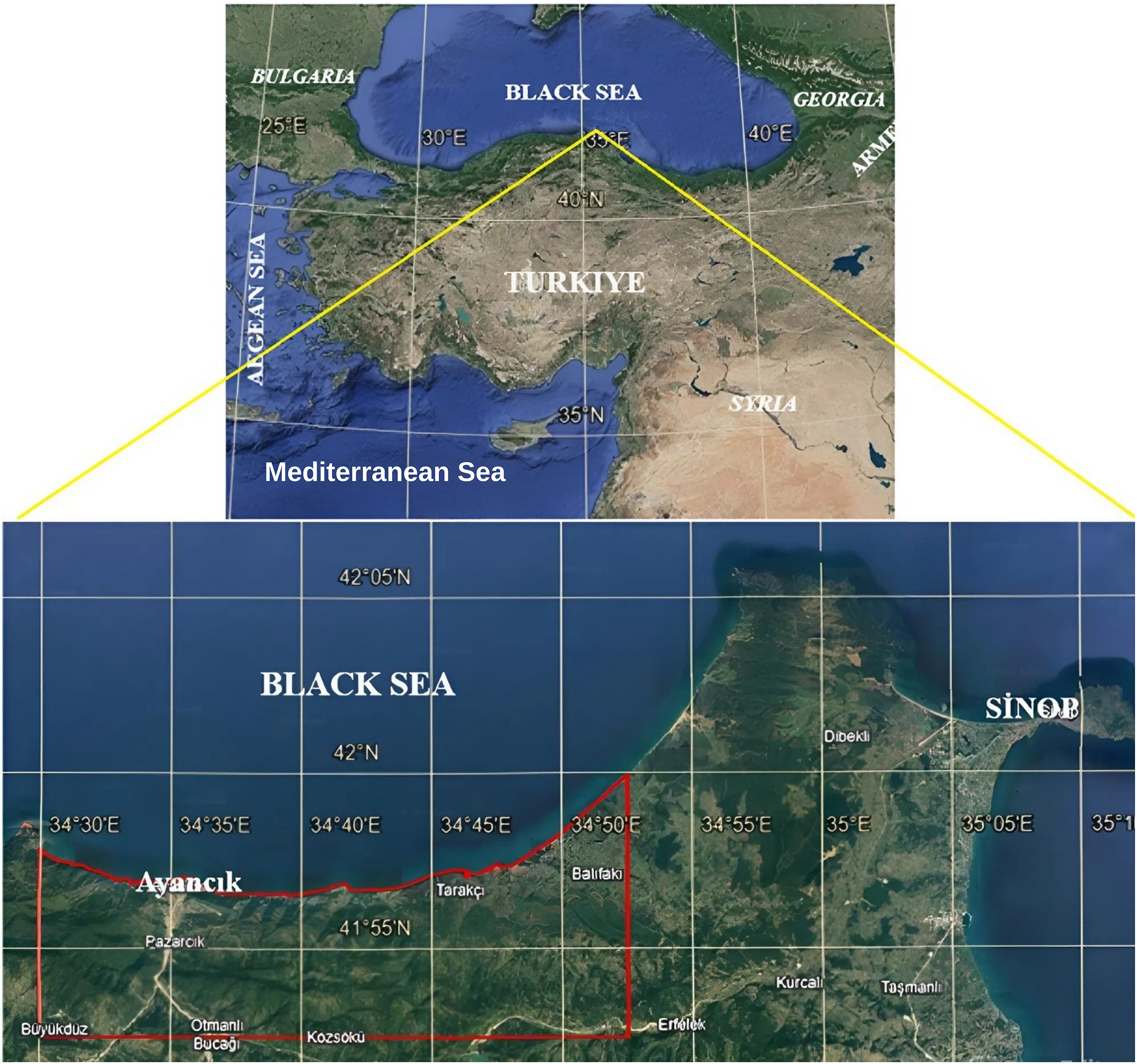
Türkiye is constantly facing the danger of natural disasters because of its geographical features and geology. Disasters such as earthquakes, landslides, floods, avalanches, drought, wildfires, extreme winter conditions, and storms often occur in Türkiye. The landslide is the most common type of all disaster events in Türkiye (32.7%) (Öcal, 2019). The study area extends between 34°30′E to 34°53′E and 41°52′30″N to 41°58′N at the western part of Sinop city in Türkiye (Fig. 1). The Black Sea region where the study area is located, has an oceanic climate with high and evenly distributed rainfall all the year round. The Black Sea region experiences year-round rainfall along the coastlines, while inland areas have a terrestrial climate with lower precipitation. The landslide records of the Disaster and Emergency Management Presidency show that the vicinity of Sinop has experienced numerous landslides (Fig. 2). The type of these landslides is generally active deep-seated rotational, and they usually occur on slopes above rivers and creeks according to the classification proposed by Cruden & Varnes (1996). Additionally, shoreline landslides are also common in the area (Akgün et al., 2012). According to Özdemir (2005), landslides can be triggered by natural environmental factors such as the geological structure of the land, terrain slope, and precipitation in the region. In addition, human activities such as incorrect land use and road construction can also disrupt the slope balance, leading to landslide occurrences. The amount of precipitation along the coastline and the valleys of the rivers flowing into the Black Sea is higher than the inland. Almost all of the landslides affecting the settlements built on lands open to marine influences in the north of the region occurred in February, March, and April, as the ground was saturated by the amount of precipitation.
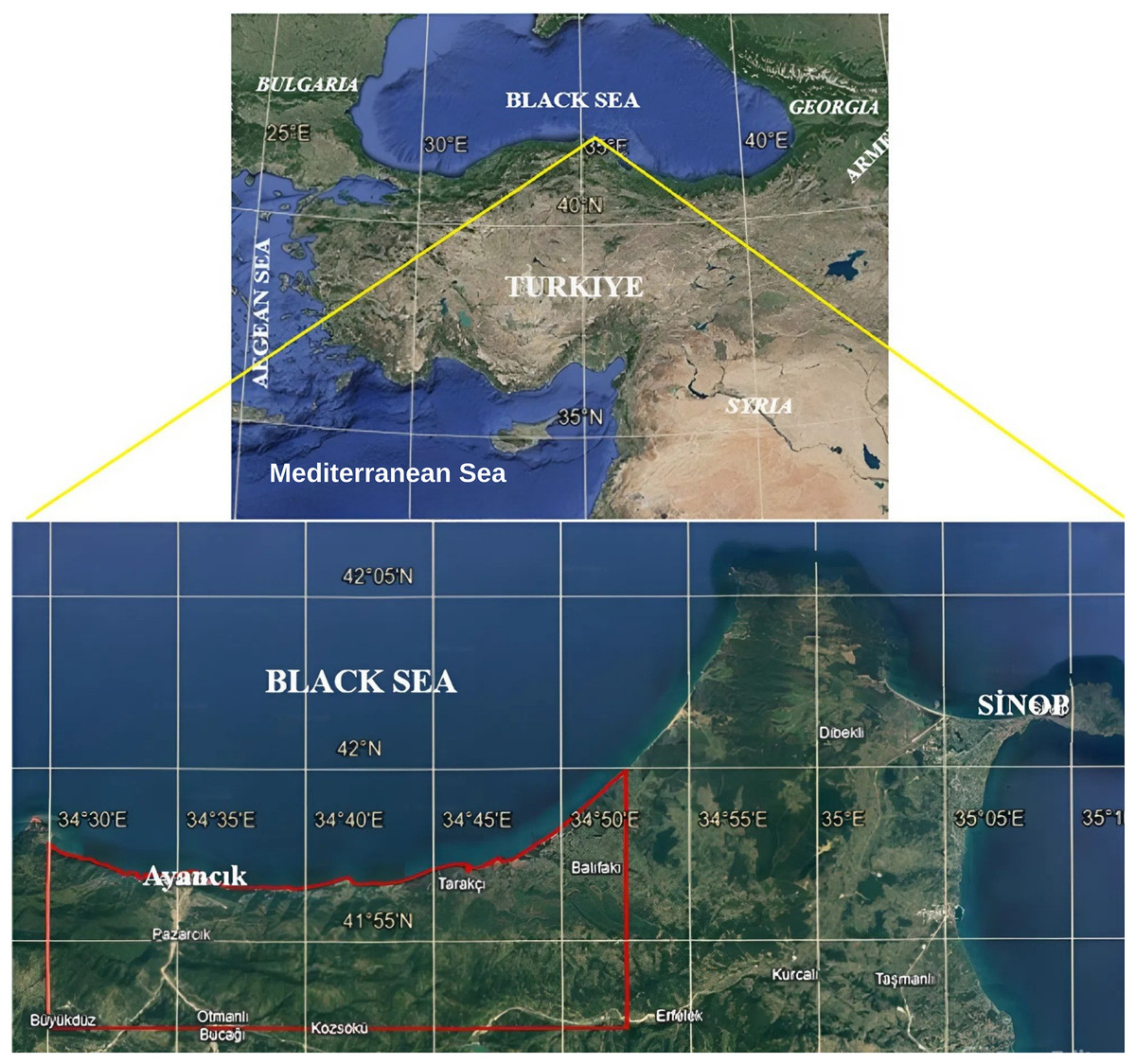
Figure 1: Location map of the study area.
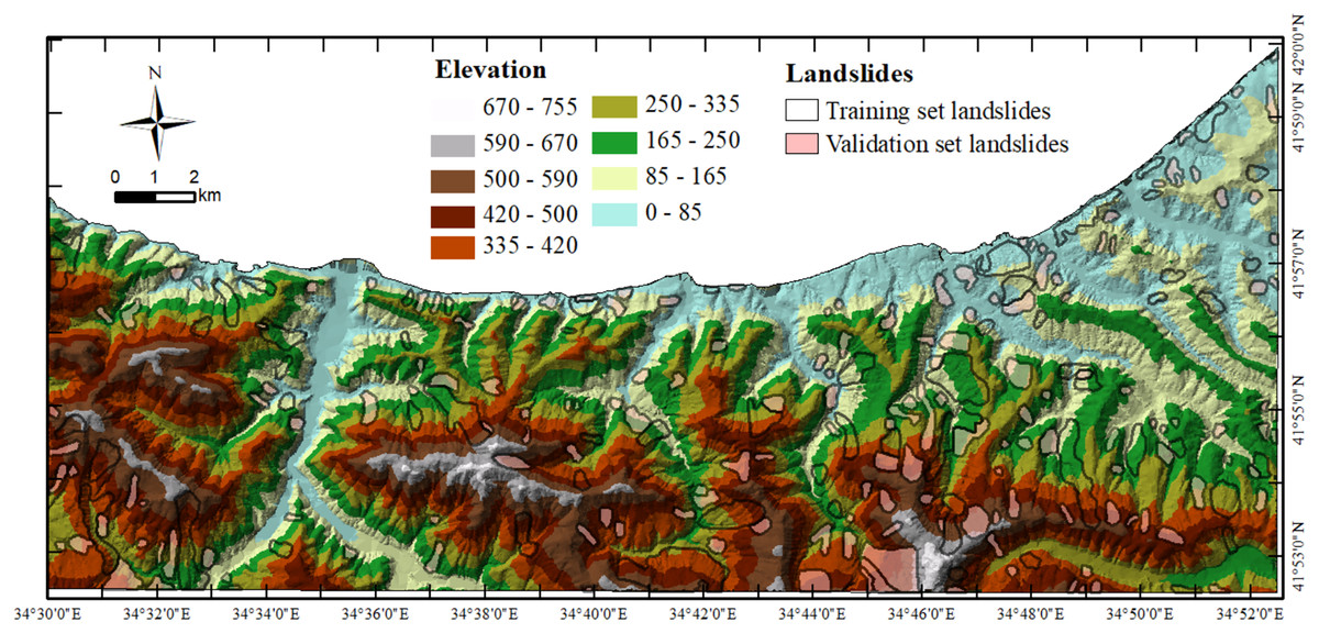
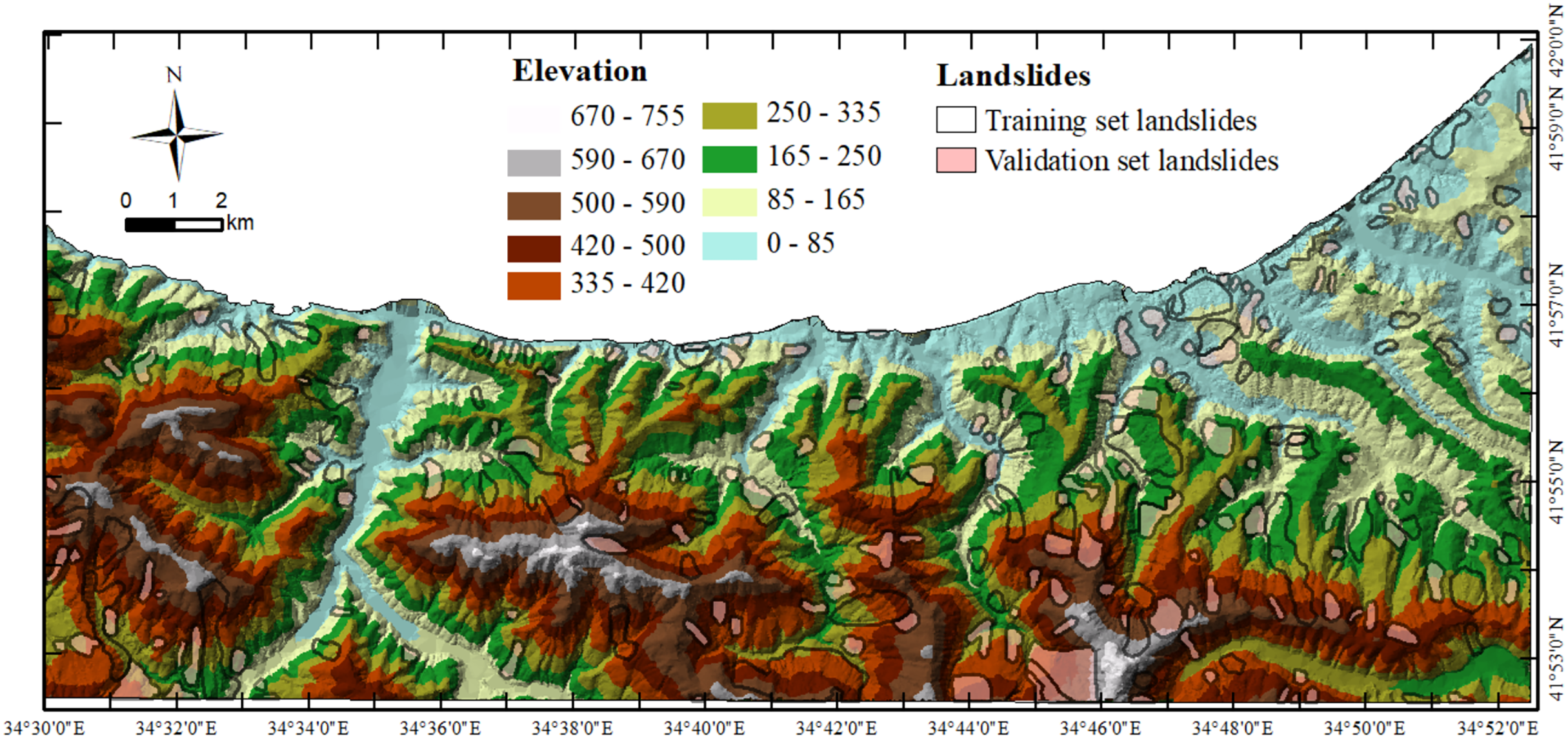
Figure 2: The distribution of validation set and training set landslides.
Spatial data
This study utilized four groups of thematic variables: geological (lithology and proximity to fault), morphological (elevation, slope, aspect, and curvature), hydrological (proximity to river), and landcover (land use and proximity to road).
For the study, several input thematic variables were considered, including lithology, elevation, slope, aspect, curvature, land use, proximity to the fault, to the road, and to the river data (Figs. 3, 4, 5). The lithology and fault data were obtained from the geological map of 1:100.000 scaled Sinop-D33 and E33 quadrangles, which were prepared by Uğuz & Sevin (2008). The road and drainage data were digitized from the 1:25.000 scaled topographic maps of the region. The maps of proximity to the fault, road, and river were prepared by using the buffer tool of the ArcGIS Desktop 10 program. The elevation, slope, aspect, and curvature maps were produced from 1:25.000 scaled digital elevation data produced by the General Directorate of Mapping (National Mapping Agency of Türkiye), by using the 3D and Spatial Analyst tools of ArcGIS Desktop 10 program. The land use map is generated from the satellite image. The landslide date was obtained from 1:25.000 scaled Landslide Inventory Map prepared by MTA (General Directorate of Mineral Research and Exploration). The same pixel size 10 × 10 is used for the raster parameter maps to eliminate uncertainties that may occur during the overlaying of raster maps. The parameters used in this study, such as lithology, slope, proximity to roads and rivers, are widely recognized in the literature as standard and essential variables in landslide susceptibility modeling (Van Westen & Bonilla, 1990; Guzzetti et al., 1999). However, their selection was not only based on common use, but also on a multi-layered evaluation tailored to the morphodynamic, lithological, and hydrological characteristics of the Sinop–Ayancık basin. For example, shallow landslides were mostly observed on formations like Kusuri, Ayancık Member, and Atbaşı, which consist of weakly cohesive and highly permeable sediments. This aligns with studies such as Reichenbach et al. (2018) and Ayalew & Yamagishi (2005), which emphasize that contact between permeable and impermeable layers is a major factor in landslide triggering due to saturation. Similarly, slope is not only analyzed in absolute values but also in relation to landslide type, slope form, and hydrological loading. Most landslides occurred on slopes between 7°–21°, matching previous findings (Uromeihy & Mahdavifar, 2000; Koukis & Ziourkas, 1991). Aspect and curvature were also considered for their amplifying effects during heavy rainfall (Ohlmacher, 2007). Proximity to rivers and roads was evaluated as a combined natural-anthropogenic trigger. Increased landslide frequency within 0–500 m of river channels is associated with toe erosion and backcutting (Choubey & Litoria, 1990; Reichenbach et al., 2018). Moreover, road construction near valleys has disturbed slope stability and altered drainage, further increasing susceptibility (Luzi & Pergalani, 1999; Van Westen, 2000). Ultimately, the selected parameters are supported not just by theory but by direct field observations and spatial analysis, strengthening the model’s regional validity and scientific robustness.
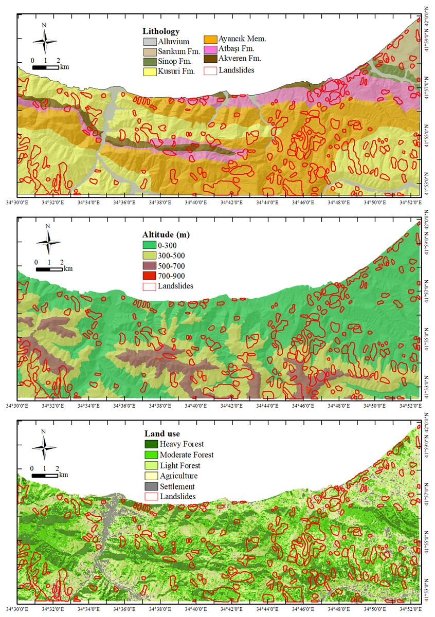
Figure 3: The parameter maps of lithology, altitude, and land use.
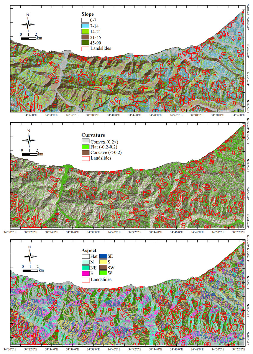
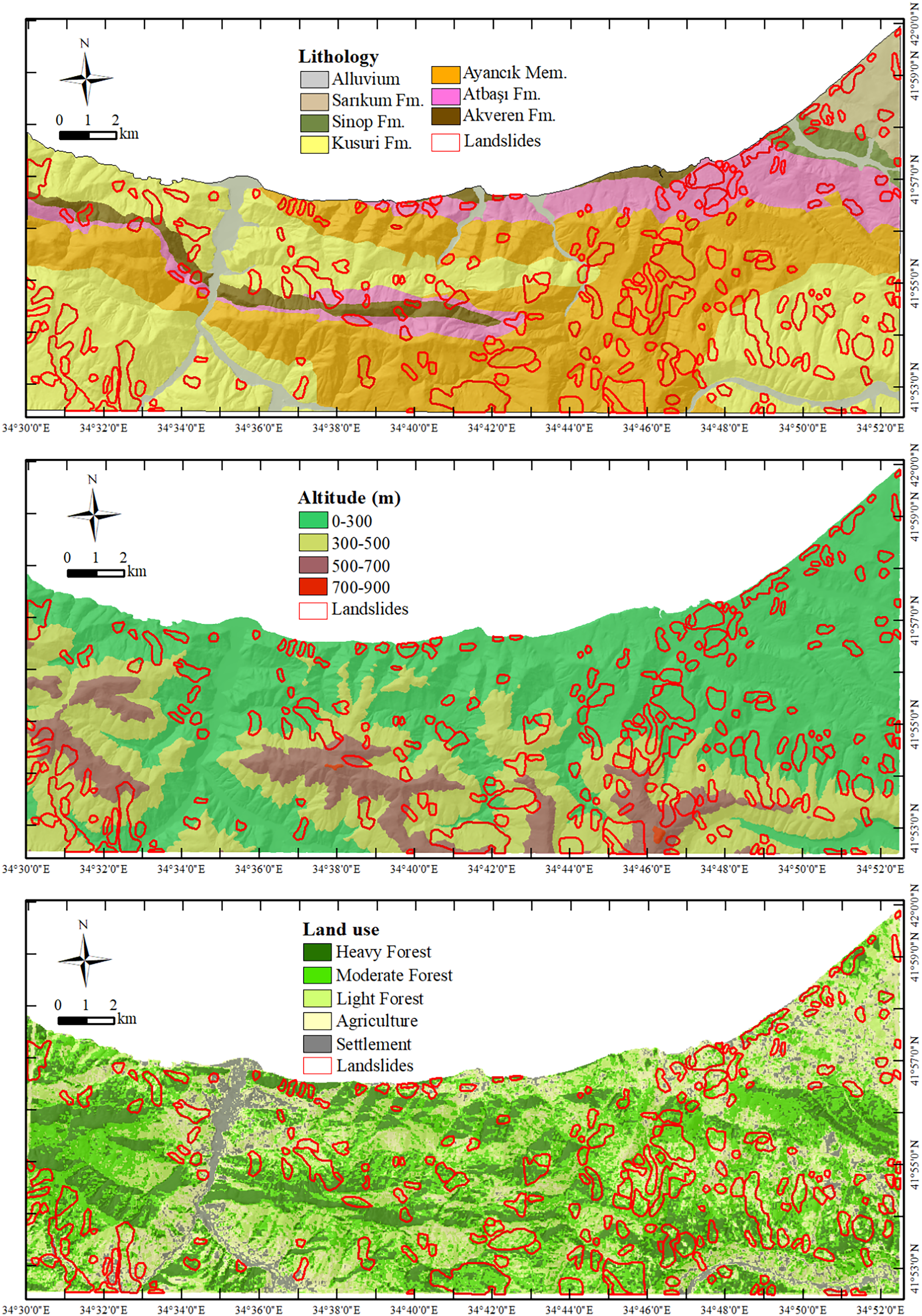
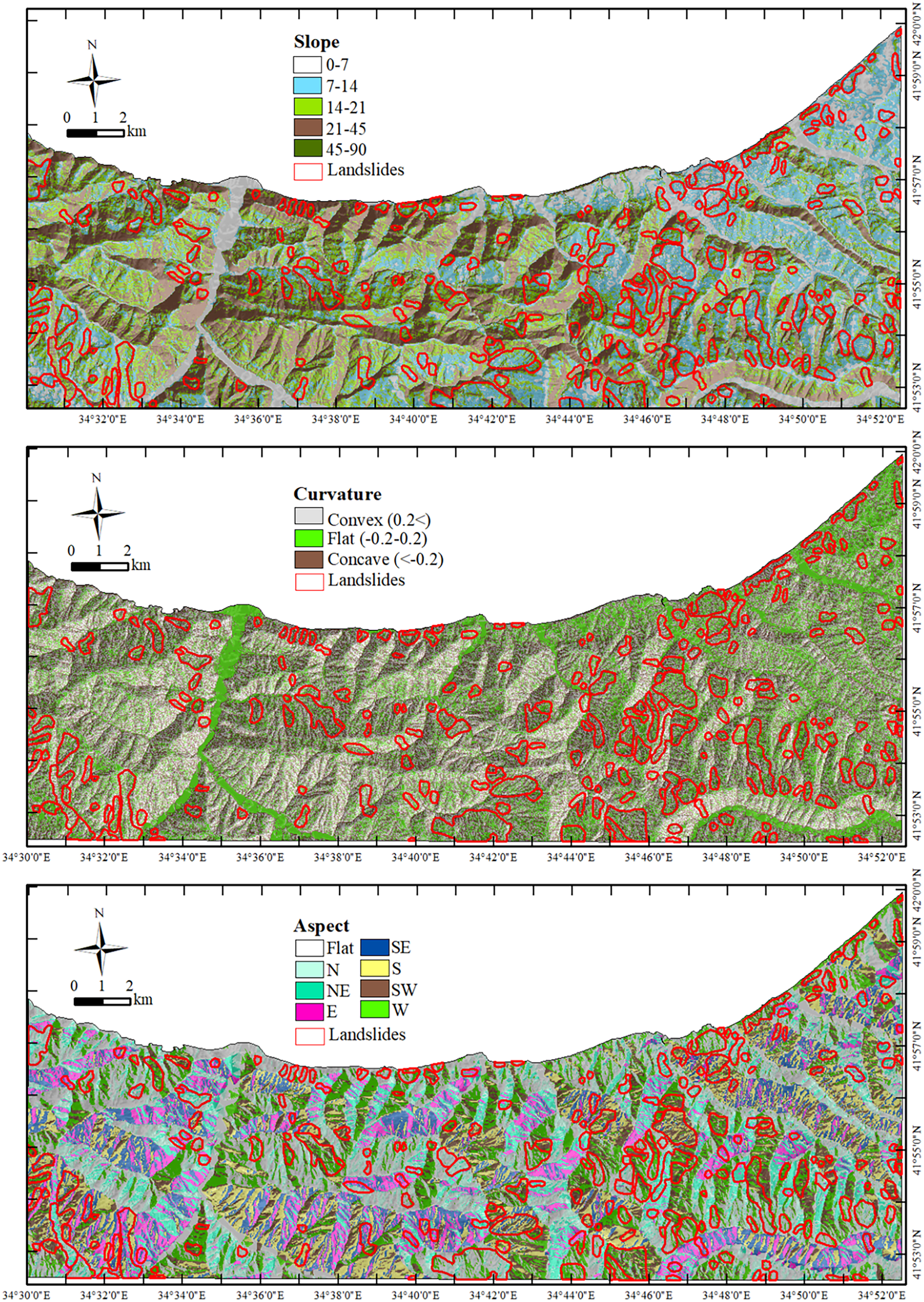
Figure 4: The parameter maps of the slope, curvature, and aspect.
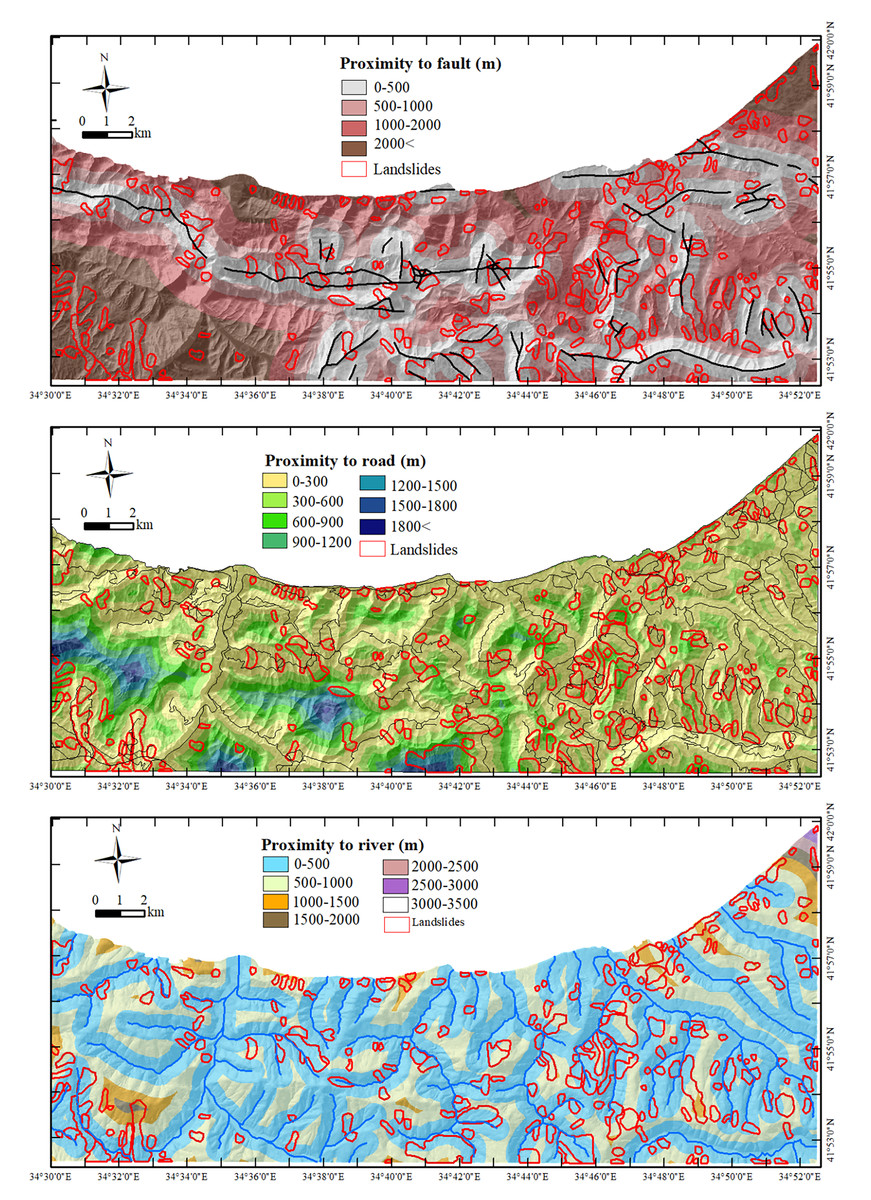
Figure 5: The parameter maps of the proximity to the fault, river, and road.
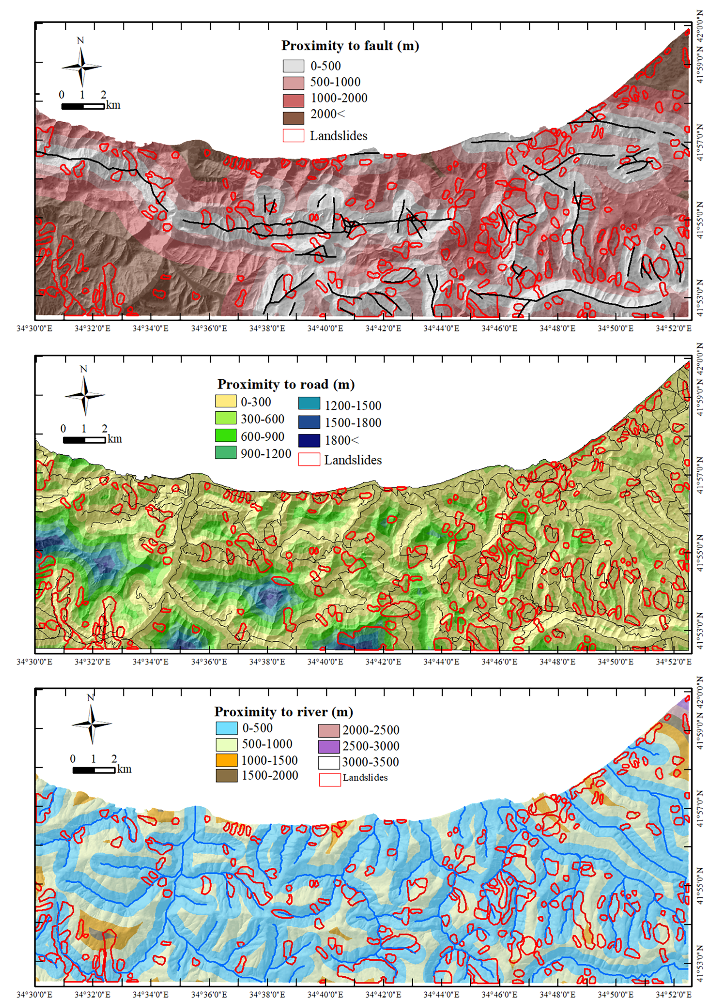
Lithology
The Sinop basin is delimited to the south by the Ekinveren thrust. Görür & Tüysüz (1997) separated the sedimentary fill of the Sinop Basin into three parts. Syn-rift, post-break-up, and post-rift units. The units outcropped in the study area are represented by post-rift deposits. The oldest unit of the study area, the Maastrichtian-Paleocene aged Akveren Formation is composed of limestone, clayey limestone, shale, claystone, siltstone, and sandstone alternations with volcanic intercalation, and was deposited open shelf-slope environment (Fig. 3). Akveren Formation overlain by Early Eocene-aged Atbaşı Formation. The Atbaşı Formation contains purple marls and shales with limestone intercalations and was deposited in an open shelf-slope environment. Lower-Middle Eocene aged Kusuri Formation and its Ayancık Member which have wide outcrops in the study area overlain the Akveren and Atbaşı formations (Sütcü et al., 1982). Kusuri Formation has a gradational lower boundary and is predominantly siliciclastic, composed of turbiditic sandstones, mudstones and minor thin marls (Aydın et al., 1995). The lower part of the Kusuri Formation consists of thick paleo-channel sandstones and conglomerates and has been referred to as the Ayancık Sandstone Member. After the attenuation of lateral movements caused by compressional regime in the region, Miocene aged Sinop Formation that compose of sandstone siltstone and claystone alternation with little amount carbonate; Late Pliocene-Early Pleistocene aged Sarıkum Formation containing sandstones with clay and mud lenses and Holocene aged fluvial deposits and coastal sand dunes were deposited in the area (Sütcü et al., 1982).
The previous studies have frequently used lithologic data for landslide susceptibility modelling. Lithology is one of the main parameters in certain areas and affect the slope stability and surface erosion in conjunction with the rock type and hardness of rock (e.g., permeable rocks overlaying impermeable sediments throughout the slope) (Reichenbach et al., 2018). In the study area, most of the landslides occurred on the Ayancık Member, Kusuri, and Atbaşı formations respectively. These units are composed of mostly sandstone, mudstone, marl, and lesser conglomerate.
Elevation
Elevation is another commonly used conditioning parameter in landslide susceptibility mapping. In the study area, the terrain rises sharply from the coastline toward the interior, except for narrow coastal plains between Erfelek and Ayancık. The eastern part of the Küre Mountains extends into Sinop, featuring hills and peaks that reach altitudes of 1,500–1,800 m in some areas. The Digital Elevation Model (DEM) was prepared using 1:25,000 scale digital elevation data. The elevation in the study area ranges from 0 to 755 m and was classified into four classes: 0–300, 300–500, 500–700, and 700–900 m (Fig. 3). Most landslides were observed at lower elevations, particularly between 0 and 300 m.
Land-cover
The land-cover parameter map was created by combining vegetation and land-use data obtained from satellite imagery. Vegetation plays an important role in preventing landslides. In particular, forests with tall trees and deep root systems help increase soil stability (Iwahashi et al., 2014). Vegetation can also regulate the amount of water that reaches the soil during rainfall. In this study, the land-cover parameter was classified into five classes: heavy forest, moderate forest, light forest, agriculture, and settlement areas. It was observed that landslides mostly occurred in areas with light and moderate forests, as well as in agricultural and settlement areas (Fig. 3).
Slope
Slope movement occurs when forces acting down-slope (mainly due to gravity) exceed the strength of the earth materials that compose the slope. Therefore, slope is an important factor for slope stability, and slope map is often used in landslide susceptibility mapping. Reichenbach et al. (2018) noted that terrain slope is the single most effective geo-environmental variable used for susceptibility modeling (Carrara et al., 1995; Fabbri et al., 2003; Budimir, Atkinson & Lewis, 2015). In the present study, the slope map was prepared from the digital elevation model (DEM) of the area and it was reclassified into five classes as 0–7°, 7–14°, 14–21°, 21–45° and 45–90° (Fig. 4).
The fact that the river valleys in the region are young has caused the valley slopes to be quite sloping. Additionally, these streams carry large amounts of load in their beds. Therefore, the erosive effects of streams increase and cause the slope balance to deteriorate. At the same time, the abundant rainfall in the region causes the rivers to change their beds very frequently, and in the meantime, the toe of the slopes is carved in many places. Landslides frequently occur on slopes where the toe is eroded (Özdemir, 2005). The terrain slope mostly ranges between 3–30° in the area, but the coastal line and valleys have higher slopes. The landslides have occurred predominantly in the areas having between 7–21° slopes in the Ayancık-Sinop region (Table 1).
| Parameter classes | Pixel counts in factor class | Pixel counts in training landslide area | Lxi/LT | Axi/AT | FRxi |
|---|---|---|---|---|---|
| Lithology | Axi | Lxi | |||
| Sinop Fm. | 37,194 | 2,821 | 1.31 | 2.14 | 0.61 |
| Akveren Fm. | 100,474 | 5,571 | 2.58 | 5.78 | 0.45 |
| Alluvium | 109,930 | 0 | 0.00 | 6.32 | 0.00 |
| Ayancık member | 111,271 | 88,755 | 41.08 | 6.40 | 6.42 |
| Kusuri Fm. | 975,165 | 83,387 | 38.60 | 56.10 | 0.69 |
| Atbaşı Fm. | 322,293 | 29,765 | 13.78 | 18.54 | 0.74 |
| Sarıkum Fm. | 81,985 | 5,731 | 2.65 | 4.72 | 0.56 |
| Total pixel (AT-LT) | 1,738,312 | 216,030 | |||
| Slope | |||||
| 0–7 | 396,728 | 23,494 | 10.88 | 14.48 | 0.75 |
| 7–14 | 762,792 | 88,542 | 40.99 | 27.84 | 1.47 |
| 14–21 | 735,629 | 61,604 | 28.52 | 26.85 | 1.06 |
| 21–45 | 839,811 | 42,189 | 19.53 | 30.65 | 0.64 |
| 45–90 | 4,780 | 187 | 0.09 | 0.17 | 0.50 |
| Total (AT–LT) | 2,739,740 | 216,016 | |||
| Aspect | |||||
| N | 553,463 | 48,038 | 22.24 | 23.63 | 0.94 |
| NE | 335,055 | 28,381 | 13.14 | 14.31 | 0.92 |
| E | 283,212 | 17,887 | 8.28 | 12.09 | 0.68 |
| SE | 252,091 | 9,402 | 4.35 | 10.76 | 0.40 |
| S | 280,857 | 12,244 | 5.67 | 11.99 | 0.47 |
| SW | 325,449 | 27,658 | 12.80 | 13.90 | 0.92 |
| W | 311,829 | 35,308 | 16.35 | 13.31 | 1.23 |
| NW | 397,784 | 37,098 | 17.17 | 16.99 | 1.01 |
| Total (AT–LT) | 2,341,956 | 216,016 | |||
| Curvature | |||||
| <−0.2 (Concave) | 938,199 | 79,824 | 36.95 | 52.57 | 0.70 |
| −0.2–0.2 (Flat) | 740,471 | 55,662 | 25.77 | 41.49 | 0.62 |
| 0.2< (Convex) | 106,107 | 80,530 | 37.28 | 5.95 | 6.27 |
| Total (AT–LT) | 1,784,777 | 216,016 | |||
| Land use | |||||
| Heavy Forest | 584,757 | 40,525 | 18.77 | 21.34 | 0.88 |
| Moderate Forest | 891,199 | 84,711 | 39.23 | 32.52 | 1.21 |
| Light Forest | 713,755 | 55,087 | 25.51 | 26.05 | 0.98 |
| Agriculture | 407,189 | 29,285 | 13.56 | 14.86 | 0.91 |
| Settlement | 143,552 | 6,308 | 2.92 | 5.24 | 0.56 |
| Total (AT–LT) | 2,740,452 | 215,916 | |||
| Proximity to the road (m) | |||||
| 0–300 | 168,992 | 142,239 | 65.83 | 13.86 | 4.75 |
| 300–600 | 625,904 | 44,462 | 20.58 | 51.35 | 0.40 |
| 600–900 | 232,488 | 9,615 | 4.45 | 19.07 | 0.23 |
| 900–1,200 | 102,177 | 8,631 | 3.99 | 8.38 | 0.48 |
| 1,200–1,500 | 59,636 | 7,476 | 3.46 | 4.89 | 0.71 |
| 1,500–1,800 | 27,945 | 3,366 | 1.56 | 2.29 | 0.68 |
| 1,800< | 1,844 | 279 | 0.13 | 0.15 | 0.85 |
| Total (AT–LT) | 1,218,986 | 216,068 | |||
| Proximity to the fault (m) | |||||
| 0–500 | 982,925 | 119,556 | 55.33 | 35.87 | 1.54 |
| 500–1,000 | 694,457 | 41,294 | 19.11 | 25.35 | 0.75 |
| 1,500–2,000 | 404,432 | 17,494 | 8.10 | 14.76 | 0.55 |
| 2,000–2,500 | 204,320 | 4,536 | 2.10 | 7.46 | 0.28 |
| 2,500–3,000 | 453,786 | 33,188 | 15.36 | 16.56 | 0.93 |
| Total (AT-LT) | 2,739,920 | 216,068 | |||
| Elevation | |||||
| 0–300 | 163,689 | 125,091 | 137.58 | 14.84 | 9.27 |
| 300–500 | 820,173 | 75,036 | 82.53 | 74.37 | 1.11 |
| 500–700 | 279,837 | 15,889 | 17.47 | 25.37 | 0.69 |
| 700–900 | 2,835 | 0 | 0.00 | 0.26 | 0.00 |
| Total (AT–LT) | 1,102,845 | 90,925 | |||
| Proximity to the river (m) | |||||
| 0–500 | 186,252 | 131,935 | 61.06 | 17.51 | 3.49 |
| 500–1,000 | 758,613 | 66,922 | 30.97 | 71.32 | 0.43 |
| 1,000–1,500 | 99,529 | 15,940 | 7.38 | 9.36 | 0.79 |
| 1,500–2,000 | 11,972 | 1,271 | 0.59 | 1.13 | 0.52 |
| 2,000–2,500 | 4,805 | 0 | 0 | 0.45 | 0 |
| 2,500–3,000 | 2,237 | 0 | 0 | 0.21 | 0 |
| 3,000–3,500 | 242 | 0 | 0 | 0.02 | 0 |
| Total (AT–LT) | 1,063,650 | 216,068 |
Curvature
The three curvature values used for hillslope and landslide analysis are profile, plan, and tangential curvature (Ohlmacher, 2007). The curvature map was prepared from the DEM data (Fig. 4) and divided into three classes: Concave (<−0.2), flat (−0.2–0.2), and convex (0.2<). The distribution of occurred landslides is almost equal in the areas with convex and concave curvatures in the study area. However, the areas with concave curvature cover a larger area than the convex and planar curvatures in the study area (Table 1).
Aspect
The aspect map of the study area is divided into eight directional classes as north (337.5–360°, 0–22.5°), northeast (22.5–67.5°), east (67.5–112.5°), southeast (112.5–157.5°), south (157.5–202.5°), southwest (202.5–247.5°), west (247.5–292.5°), and northwest (292.5–337.5°) (Fig. 4). The distribution of landslides on different aspects is generally uniform in the area, although there are slightly more landslide occurrences on slopes facing N and NW directions. Reichenbach et al. (2018) indicated that aspect data is less justified, theoretically and empirically, and maybe controlled by local conditions.
Proximity to the fault
Tepecik-Yenice, Balıfakı-Hamidiye and Erikli faults are the most important faults in the area. They are reverse faults and extend E-W direction. There are also small normal faults with about N-S direction in the region (Uğuz & Sevin, 2008). Faults caused seismic activities, tectonic breaks and decreasing of rock strength, are responsible for triggering a large number of landslides. The proximity to fault map was prepared with 500 m buffer zones (Fig. 5). The distribution of the landslides is very close to the fault lines in the area and most of the landslides occurred in the 0–500 m buffer zone of the fault line.
Proximity to the river
The Ayancık, Büyük, Yenice, Kocaköyyalısı, and Baba streams, along with their tributaries, play a significant role in shaping the region’s topography. The rivers in the study area form a dendritic-type drainage system, where numerous sub-tributaries merge into the main river channels. In the western part of the study area, the river valley slopes are steeper, while in the eastern part where most landslides occurred the slopes are gentler.
Drainage density and land saturation levels are important factors in slope stability. Rivers can erode nearby slopes or saturate their bases until water pressure builds up. Proximity to river segments indicates areas prone to sediment movement and erosion. In this study, proximity to rivers was used as one of the conditioning parameters. The proximity map was created using buffer zones at 500-m intervals based on drainage data (Fig. 5). Most landslides were found within the 0–500 m buffer zone, a pattern similar to that observed for the proximity to fault parameter.
Proximity to the road
Landslides can result from slope destabilization due to road construction. A significant number of landslides in the study area occur on the roadsides of the Sinop-Ayancık-Türkeli coastal road, the Sinop-Samsun highway, and village roads (Fig. 5). These roads are closed frequently to traffic as a result of landslides. Therefore, the study used proximity to the road as a triggering parameter. The buffer zone map was prepared from the road data (Fig. 5). Most of the landslides are located within the map’s 0–500 m buffer zone.
Methodology
Data preprocessing and dataset structure
The dataset utilized in this research was collected from field observations, geological surveys, and existing geological maps covering the cities of Sinop and Ayancık, Türkiye. Data were gathered specifically on lithological units (such as Sinop Formation, Akveren Formation, Alüvyon Formation, and Ayancık), and occurrences of landslide events within these geological formations were recorded.
The dataset consists of several key components:
Class and Lithology: Geological formations were categorized into distinct lithological classes based on geological characteristics observed in the field.
Variable Counts: The total area covered by each lithological class (“Count in the variable class”) and the occurrence of landslides within each class (“Count in the landslide test area”) were quantified using GIS spatial analyses.
Susceptibility Index: Calculated to assess the relative likelihood of landslide occurrences within the defined lithological classes.
For consistency and comparability, all three methods classify landslide susceptibility into five standard zones: very low, low, moderate, high, and very high. This classification facilitates interpretation and visual mapping across methods.
The collected spatial data were digitized, georeferenced, and processed using Geographic Information Systems (GIS) software such as ArcGIS or QGIS. This step involved converting raw spatial data into raster layers suitable for further statistical analyses and modeling.
For model development, the landslide inventory data was randomly split into training and validation sets, consistent with standard practice in statistical susceptibility modeling.
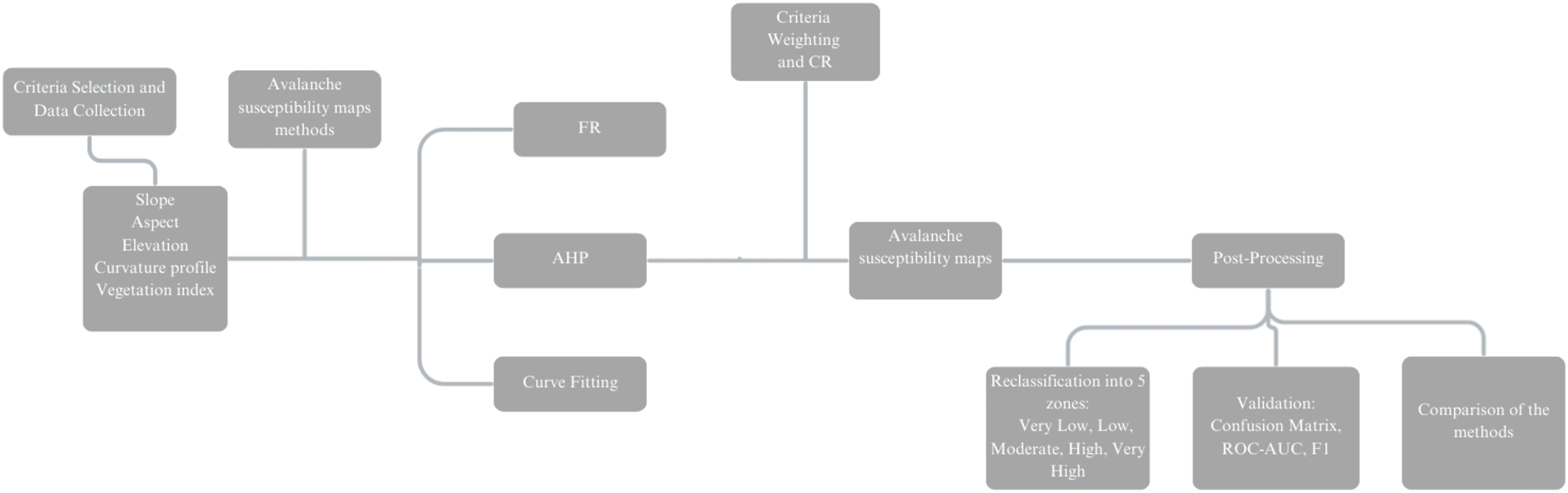
The overall methodology followed in this study is summarized in Fig. 6. The process begins with the selection and collection of spatial data layers, including slope, aspect, elevation, curvature, and land cover, derived from satellite imagery, topographic maps, and geological surveys. These layers are pre-processed by converting to raster format, classified into meaningful intervals, and aligned spatially in a GIS environment. The selected conditioning factors are then input into three different modeling approaches: FR, AHP, and Curve Fitting. For AHP, additional steps such as criteria weighting and consistency ratio (CR) analysis are conducted. All models produce individual landslide susceptibility maps, which are then validated using confusion matrix, ROC-AUC, and F1-score metrics.
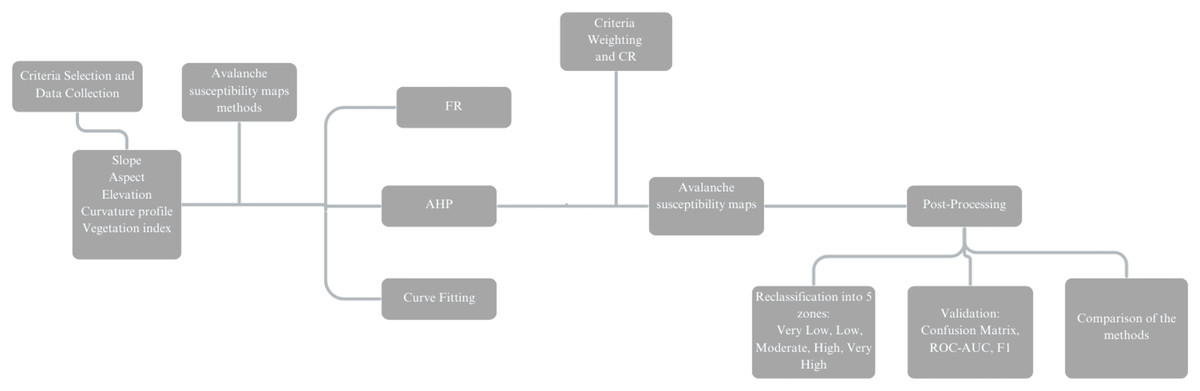
Figure 6: Workflow of data processing, modeling, and validation used in the preparation of landslide susceptibility maps.
All spatial analyses and map production were performed using ArcGIS Desktop 10 and QGIS for raster processing and visualization. The analytical models were implemented using Python 3.10, with key libraries including NumPy, SciPy, pandas, and scikit-learn. The curve fitting method was coded using SciPy’s non-linear least squares function. All computations were run on a Windows-based workstation with an Intel Core i7 processor, 32 GB RAM, and a 64-bit operating system. The AHP matrix and consistency ratio calculations were conducted using Microsoft Excel with manual pairwise input.
Frequency ratio method
The FR method is based on the relationship between the spatial distribution of landslides and the conditioning parameters. Landslides from the inventory data were divided into two groups: training and validation (control) sets. The training set was used to calculate the frequency ratios of the parameter classes. Different strategies can be used to split training and validation sets, depending on the validation type. In the literature, temporal, spatial, and random selection methods have been applied (Reichenbach et al., 2018). In this study, random selection was used, as it is commonly preferred in previous research for model performance validation.
The conditioning parameters used to generate the landslide susceptibility map included lithology, elevation, slope, aspect, curvature, proximity to fault lines, rivers, and roads, as well as land cover. The frequency ratios of these parameter classes and the Landslide Susceptibility Index (LSI) were calculated according to Eqs. (1) and (2).
Based on Eq. (1), the frequency ratio for each parameter class is calculated by using variables, Lxi, LT, Axi, and AT. Then the resultant FR values were assigned to the corresponding classes of the raster parameter maps. The data of parameter classes and calculated FR values are listed in Table 1.
(1)
FRxi = The frequency ratio in class i of parameter x
Lxi = Number of pixels in the training landslides area occupied by class i of x parameter
Axi, = Number of pixels in the class i of x parameter
LT = Total number of pixels in the training landslides area.
AT = Total number of pixels in the study area.
The landslide susceptibility index measures the likelihood of landslides occurring in a particular area. This index is calculated by overlaying raster maps of the parameters and summing them based on Eq. (2). The FR value of each class in the parameter maps is considered to be a weight value for the related class. Each pixel value in the resulting raster map represents the LSI value for a specific spatial location on the map. The area/pixel that has a higher LSI value on the resulting output raster will be more susceptible to landslide.
(2)
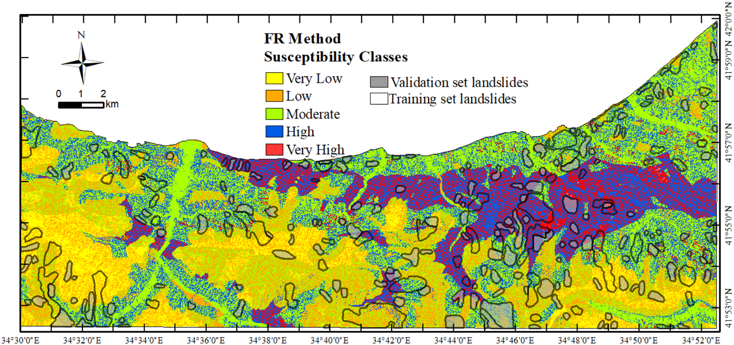
The frequency ratio of each parameter class was accepted as the weight value of each class. Each pixel value of the raster susceptibility map was assumed as the LSI of the spatial location on the map. The LSI values of the resultant map ranges from 4.26 to 31.12, with a mean of 13.39 and a standard deviation of 4.34. The LSI values are classified into five classes: very high, high, moderate, low, and very low susceptibility index to make it easier to interpret (Fig. 7). High LSI values indicate more susceptibility for the landslide occurrence.
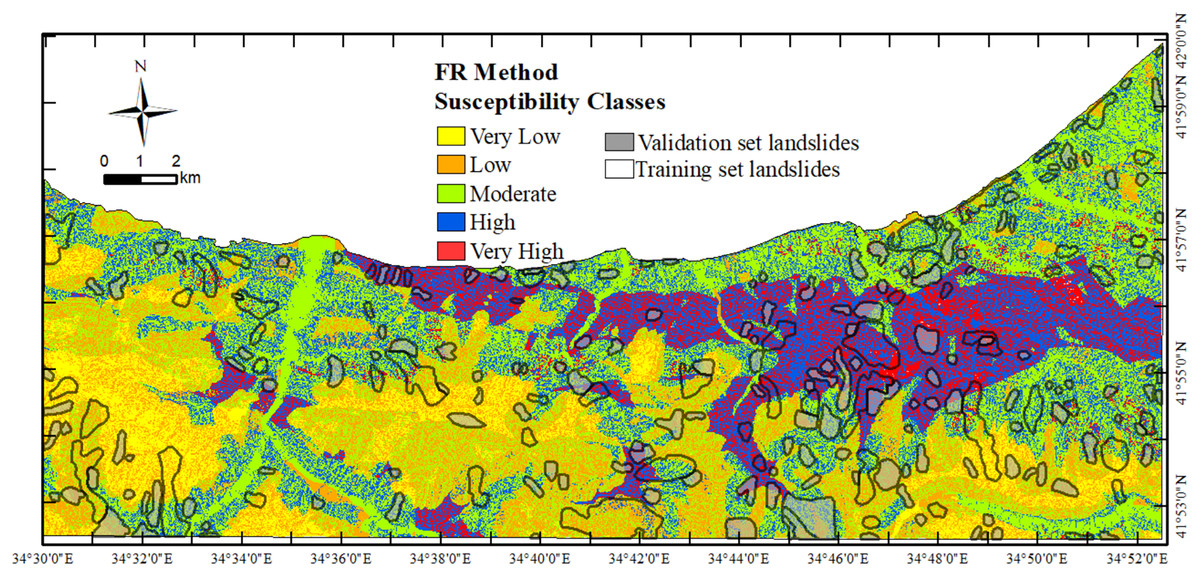
Figure 7: The landslide susceptibility map prepared from the frequency ratio method.
Analytical hierarchy process (AHP) method
The AHP, developed by Saaty (1980), provides a flexible and easily understood method for analyzing complex problems. It is widely used in group decision-making across various fields such as government, business, industry, healthcare, and education. AHP is a subjective method used in landslide susceptibility evaluation, relying on expert knowledge to determine the parameters affecting landslide processes. It is used to identify the relative importance of each criterion (parameter) and sub-criterion (class) contributing to landslide susceptibility by assigning weights.
This is done by constructing a hierarchy of decision criteria and performing pair-wise comparisons in a matrix where each parameter is rated against the others by assigning a score. The scores range from 1 to 9, as shown in Table 2. In this matrix, if the parameter on the vertical axis is more significant than the one on the horizontal axis, a value between 1 and 9 is given
| Preference factor | Degree of preference | Explanation |
|---|---|---|
| 1 | Equally | Two factors contribute equally to the objective |
| 3 | Moderately | Experience and judgment slightly to moderately favor one factor over another |
| 5 | Strongly | Experience and judgment strongly or essentially favor one factor over another |
| 7 | Very strongly | A factor is strongly favored over another and its dominance is showed in practice |
| 9 | Extremely | The evidence of favoring one factor over another is of the highest degree possible of an affirmation |
| 2, 4, 6, 8 | Intermediate | Used to represent compromises between the preferences in weights 1, 3, 5, 7 and 9 |
| Reciprocals | Opposites | Used for inverse comparison |
In AHP, an index of consistency, known as the CR, indicates the probability that the matrix judgments were randomly generated (Saaty, 1977). If the CR value is greater than 0.1, the parameter is eliminated. Using a weighted linear sum procedure, the acquired weights used for calculating the landslide susceptibility models (Komac, 2006).
where RI is the average of the resulting consistency index depending on the order of the matrix given by Saaty (1977) (Table 3). CI is the consistency index and it is expressed as
where λmax is the largest or principal eigenvalue of the matrix and can be easily calculated from the matrix, and n is the order of the matrix.
| N | 1 | 2 | 3 | 4 | 5 | 6 | 7 | 8 | 9 | 10 | 11 | 12 | 13 | 14 | 15 |
|---|---|---|---|---|---|---|---|---|---|---|---|---|---|---|---|
| RI | 0 | 0 | 0.58 | 0.90 | 1.12 | 1.24 | 1.32 | 1.41 | 1.45 | 1.49 | 1.51 | 1.53 | 1.56 | 1.57 | 1.59 |
After creating the pairwise comparison matrix, weights of the parameter classes and consistency ratios of the parameters were calculated (Table 4).
| Parameter classes | |||||||||
|---|---|---|---|---|---|---|---|---|---|
| Lithology | Weight | ||||||||
| Sinop Fm. | 1 | 0.245 | |||||||
| Akveren Fm. | 1 | 1 | 0.245 | ||||||
| Ayancık Mem. | 1/3 | 1/3 | 1 | 0.085 | |||||
| Kusuri Fm. | 1/2 | 1/2 | 2 | 1 | 0.129 | ||||
| Atbaşı Fm. | 1 | 1 | 3 | 2 | 1 | 0.235 | |||
| Sarıkum Fm. | 1/4 | 1/4 | 1/2 | 1/2 | 1/3 | 1 | 0.061 | ||
| CR | 0.008 | ||||||||
| Slope | |||||||||
| 0–7 | 1 | 0.157 | |||||||
| 7–14 | 3 | 1 | 0.448 | ||||||
| 14–21 | 2 | 1/2 | 1 | 0.178 | |||||
| 21–45 | 1/2 | 1/5 | 1 | 1 | 0.109 | ||||
| >45 | 1/2 | 1/5 | 1 | 1 | 1 | 0.109 | |||
| CR | 0.053 | ||||||||
| Aspect | |||||||||
| N | 1 | 0.052 | |||||||
| NE | 2 | 1 | 0.080 | ||||||
| E | 2 | 1 | 1 | 0.088 | |||||
| SE | 4 | 4 | 4 | 1 | 0.225 | ||||
| S | 1 | 1 | 1/2 | 1/2 | 1 | 0.067 | |||
| SW | 1 | 1/2 | 1/2 | 1/4 | 1 | 1 | 0.056 | ||
| W | 3 | 2 | 2 | 1/2 | 2 | 2 | 1 | 0.138 | |
| NW | 5 | 4 | 4 | 2 | 4 | 4 | 2 | 1 | 0.294 |
| CR | 0.022 | ||||||||
| Curvature | |||||||||
| <−0.2 (Concave) | 1 | 0.297 | |||||||
| −0.2–0.2 (Flat) | 1/2 | 1 | 0.164 | ||||||
| 0.2< (Convex) | 2 | 3 | 1 | 0.539 | |||||
| CR | 0.009 | ||||||||
| Land-cover | |||||||||
| Heavy forest | 1 | 0.062 | |||||||
| Moderate forest | 2 | 1 | 0.099 | ||||||
| Light forest | 3 | 2 | 1 | 0.161 | |||||
| Agriculture | 4 | 3 | 2 | 1 | 0.262 | ||||
| Settlement | 5 | 4 | 3 | 2 | 1 | 0.416 | |||
| CR | 0.015 | ||||||||
| Proximity to the road (m) | |||||||||
| 0–500 | 1 | 0.311 | |||||||
| 500–1,000 | 1/2 | 1 | 0.191 | ||||||
| 1,000–1,500 | 1/3 | 1/2 | 1 | 0.099 | |||||
| 1,500–2,000 | 1/3 | 1/2 | 1 | 1 | 0.099 | ||||
| 2,000–2,500 | 1/3 | 1/2 | 1 | 1 | 1 | 0.099 | |||
| 2,500–3,000 | 1/3 | 1/2 | 1 | 1 | 1 | 1 | 0.099 | ||
| 3,000< | 1/3 | 1/2 | 1 | 1 | 1 | 1 | 1 | 0.099 | |
| CR | 0.055 | ||||||||
| Proximity to the fault (m) | |||||||||
| 0–500 | 1 | 0.351 | |||||||
| 500–1,000 | 1/2 | 1 | 0.209 | ||||||
| 1,500–2,000 | 1/3 | 1/2 | 1 | 0.110 | |||||
| 2,000–2,500 | 1/3 | 1/2 | 1 | 1 | 0.110 | ||||
| 2,500–3,000 | 1/3 | 1/2 | 1 | 1 | 1 | 0.110 | |||
| CR | 0.002 | ||||||||
| Elevation (m) | |||||||||
| 0–300 | 1 | 0.482 | |||||||
| 300–500 | 1/2 | 1 | 0.272 | ||||||
| 500–700 | 1/3 | 1/2 | 1 | 0.158 | |||||
| 700–900 | 1/5 | 1/3 | 1/2 | 1 | 0.088 | ||||
| CR | 0.005 | ||||||||
| Proximity to the river (m) | |||||||||
| 0–500 | 1 | 0.361 | |||||||
| 500–1,000 | 1/2 | 1 | 0.257 | ||||||
| 1,000–1,500 | 1/3 | 1/2 | 1 | 0.126 | |||||
| 1,500–2,000 | 1/4 | 1/3 | 1/2 | 1 | 0.070 | ||||
| 2,000–2,500 | 1/5 | 1/5 | 1/2 | 1 | 1 | 0.063 | |||
| 2,500–3,000 | 1/5 | 1/5 | 1/2 | 1 | 1 | 1 | 0.063 | ||
| 3,000–3500 | 1/7 | 1/5 | 1/2 | 1 | 1 | 1 | 1 | 0.060 | |
| CR | 0.008 | ||||||||
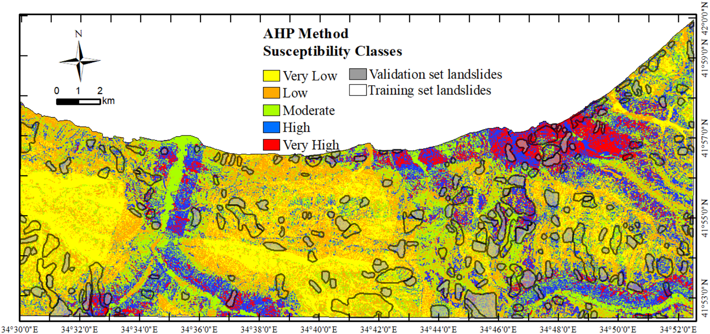
The weights of the classes were used to produce the landslide susceptibility map of the area (Table 4). Each pixel value of the resultant raster map was defined as the landslide susceptibility index of the spatial location in the map. The landslide susceptibility index values range from 0.94 to 3.40, the mean is 1.20, and the standard deviation is 0.36. The susceptibility index values were classified into five groups: very high, high, moderate, low, and very low susceptibility to facilitate easy interpretation. The high LSI values indicate more susceptible areas to the landslides (Fig. 8).
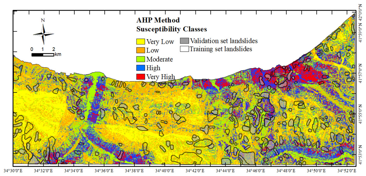
Figure 8: The landslide susceptibility map prepared from the AHP method.
Curve fitting method
The Curve Fitting method was employed to develop a mathematical model that predicts landslide susceptibility based on specific conditioning parameters. In this approach, we defined variables , and as follows:
= Class number of the conditioning parameter (e.g., slope class, lithology class).
= Total number of pixels in the study area
= Total number of pixels in the training landslides area.
The methodology involved fitting a custom function to model the relationship between these variables:
(3) where:
, c and d are parameters to be estimated.
is the natural logarithm of .
Using Python’s SciPy library, we performed non-linear least squares fitting to estimate the parameters.
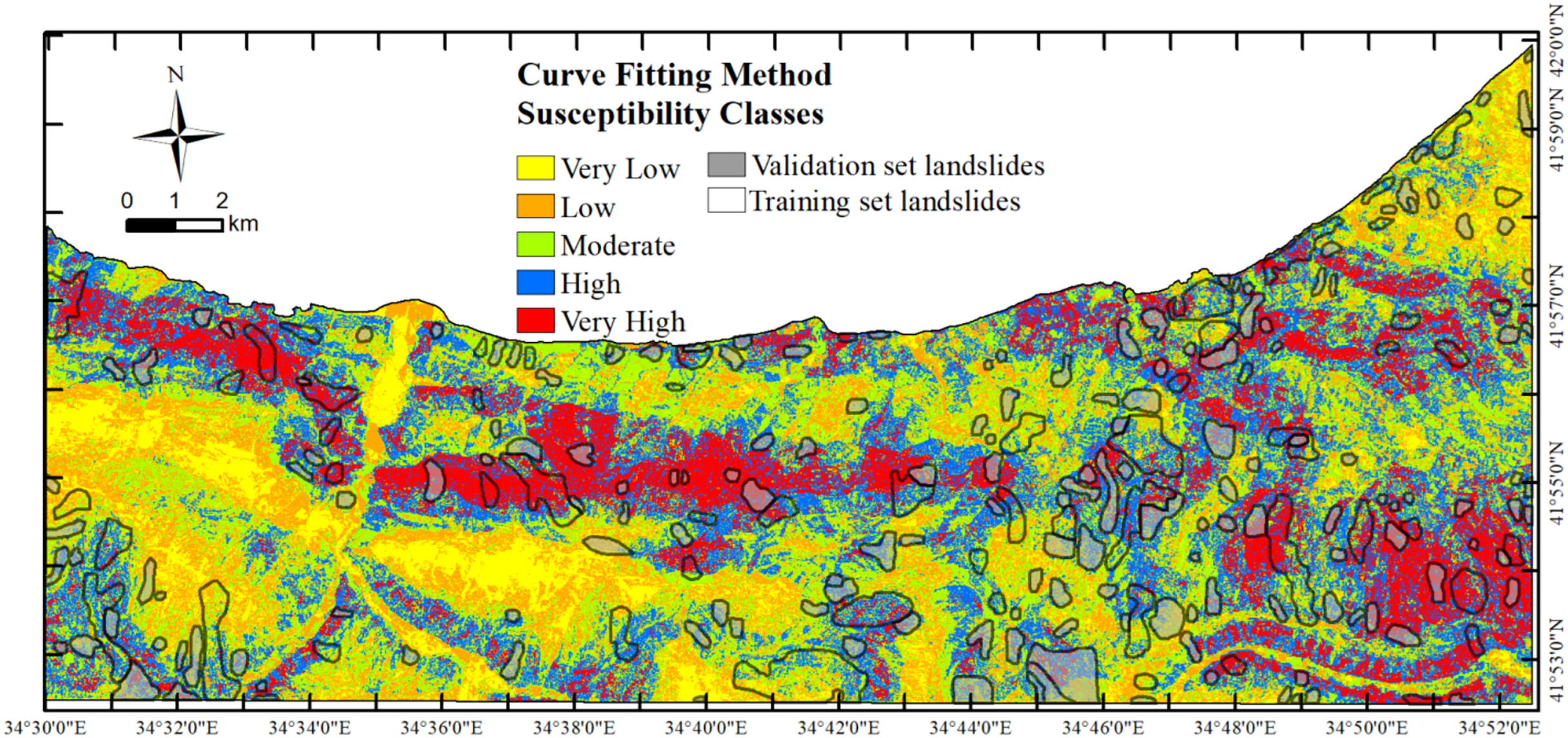
The calculated parameter values are listed (Table 5). The parameter class values were used to generate the landslide susceptibility map of the study area. Each pixel in the resulting raster map represents the Landslide Susceptibility Index (LSI) at that spatial location. The LSI values range from 1.90 to 9, with a mean of 6.23 and a standard deviation of 0.99. These values were classified into five categories: very high, high, moderate, low, and very low susceptibility. Higher LSI values indicate areas more prone to landslides (Fig. 9).
| Susceptibility classes | FR | AHP | Curve fitting |
|---|---|---|---|
| Percentage of susceptibility class area in the validation landslides | Percentage of susceptibility class area in the validation landslides | Percentage of susceptibility class area in the validation landslides | |
| Very low | 10.43 | 7.31 | 3.72 |
| Low | 26.00 | 23.20 | 14.44 |
| Moderate | 11.81 | 30.35 | 28.59 |
| High | 36.57 | 26.64 | 33.48 |
| Very high | 15.18 | 12.51 | 19.77 |
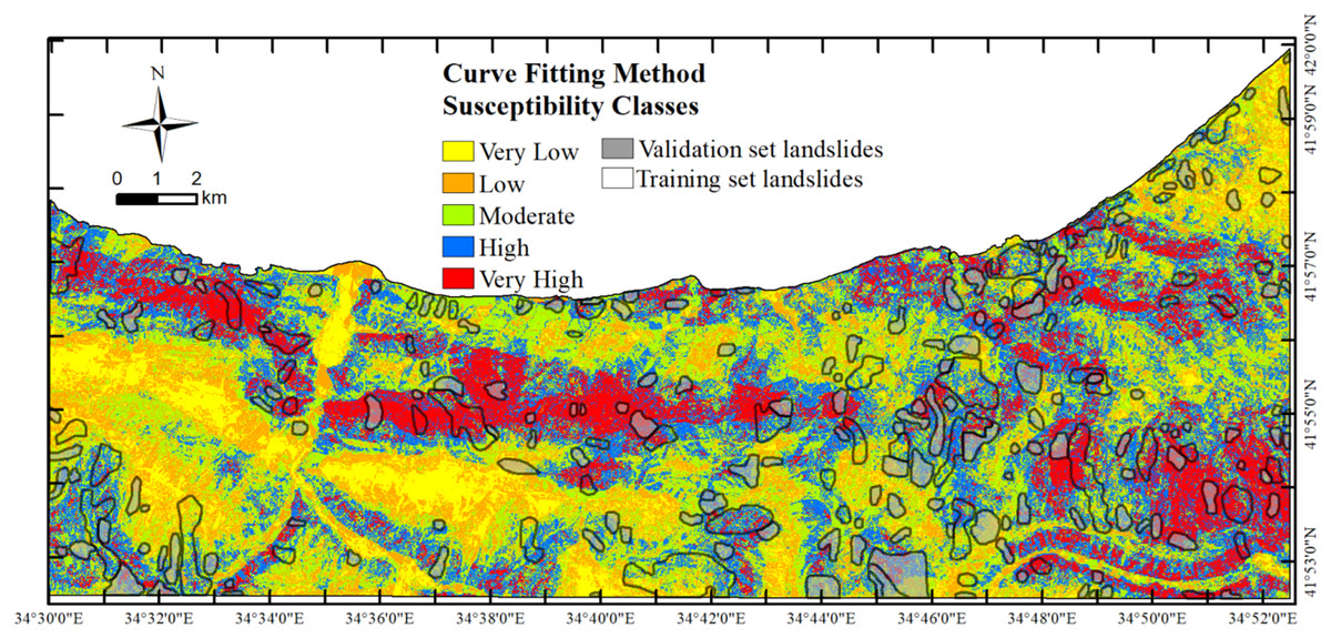
Figure 9: The landslide susceptibility map prepared from the curve fitting method.
The Python script and dataset used for curve fitting are publicly available at DOI: 10.5281/zenodo.16577952.
Results
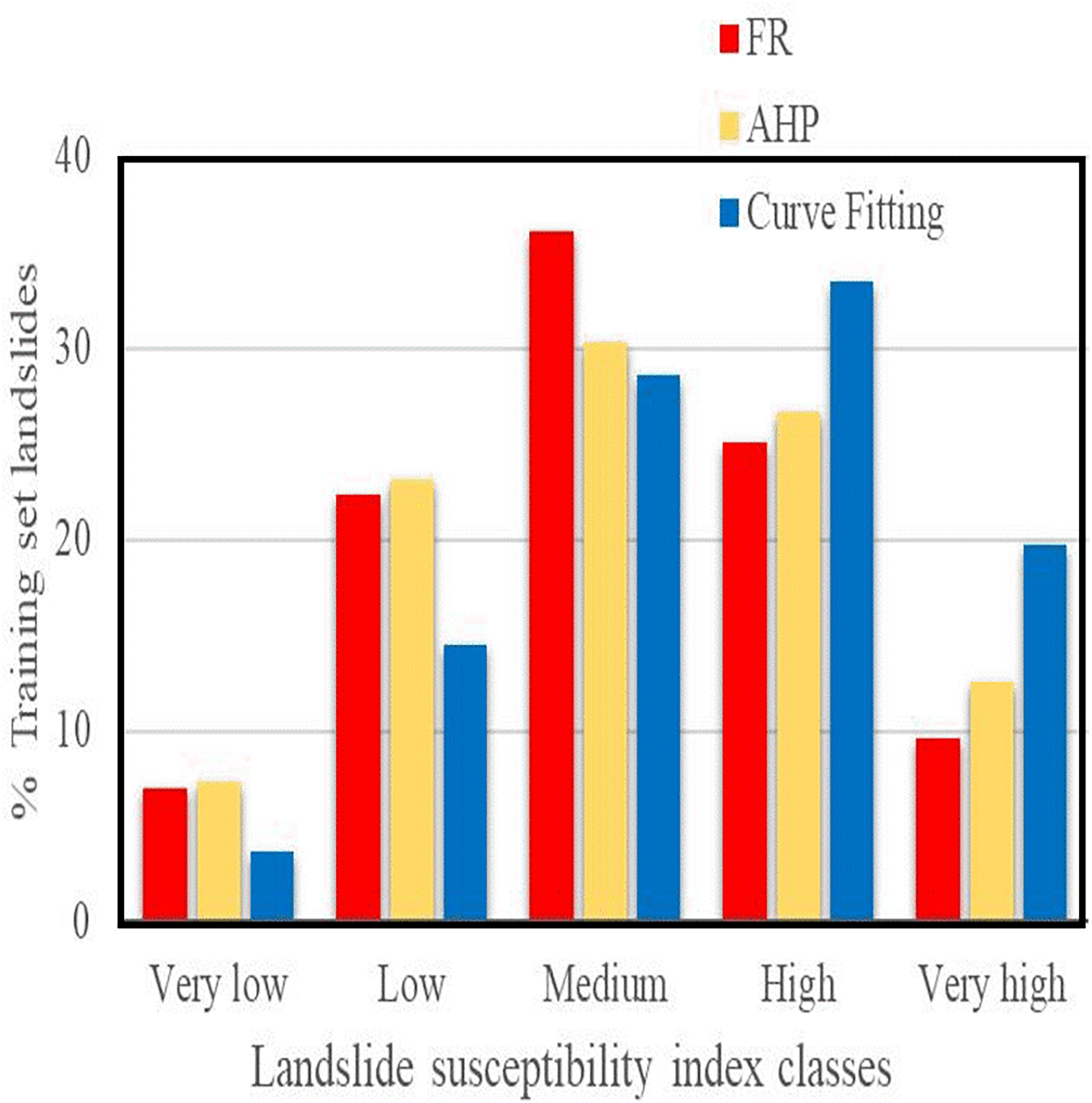
The validations of the landslide susceptibility maps were carried out using the validation (control) set landslides for each method. The distribution of landslides across the five susceptibility classes provides a qualitative assessment of the model results (Table 6). The methods showed differences in how the validation landslides were distributed among the classes. Specifically, 51.75%, 39.15%, and 53.25% of the validation landslides were located in the very high and high susceptibility classes for the FR, AHP, and Curve Fitting methods, respectively. Additionally, 11.81%, 30.15%, and 28.59% of the validation landslides fell within the moderate susceptibility class according to the FR, AHP, and Curve Fitting methods, respectively (Table 6 and Fig. 10).
| Parameter classes | Pixel counts in factor class | Pixel counts in training landslide area | Curve fitting values |
|---|---|---|---|
| Lithology | Axi | Lxi | |
| Sinop Fm. | 37,194 | 2,821 | 105.64 |
| Akveren Fm. | 100,474 | 5,571 | 22,891.40 |
| Alluvium | 109,930 | 0 | 24,953.74 |
| Ayancık member | 111,271 | 88,755 | 25,231.76 |
| Kusuri Fm. | 975,165 | 83,387 | 75,002.37 |
| Atbaşı Fm. | 322,293 | 29,765 | 49,616.60 |
| Sarıkum Fm. | 81,985 | 5,731 | 18,228.49 |
| Slope | |||
| 0–7 | 396,728 | 23,494 | 35,429.83 |
| 7–14 | 762,792 | 88,542 | 62,127.58 |
| 14–21 | 735,629 | 61,604 | 76,990.88 |
| 21–45 | 839,811 | 42,189 | 42,915.18 |
| 45< | 4,780 | 187 | −1,447.47 |
| Aspect | |||
| N | 553,463 | 48,038 | 1 |
| NE | 335,055 | 28,381 | 0.516777143 |
| E | 283,212 | 17,887 | 0.319381526 |
| SE | 252,091 | 9,402 | 0 |
| S | 280,857 | 12,244 | 0.309689771 |
| SW | 325,449 | 27,658 | 0.548154692 |
| W | 311,829 | 35,308 | 0.548637564 |
| NW | 397,784 | 37,098 | 0.750043001 |
| Curvature | |||
| <−0.2 (Concave) | 938,199 | 79,824 | 0.971610101 |
| −0.2–0.2 (Flat) | 740,471 | 55,662 | 0 |
| 0.2< (Convex) | 106,107 | 80,530 | 1 |
| Land-cover | |||
| Heavy forest | 584,757 | 40,525 | 0.525091 |
| Moderate forest | 891,199 | 84,711 | 1 |
| Light forest | 713,755 | 55,087 | 0.840084 |
| Agriculture | 407,189 | 29,285 | 0.285061 |
| Settlement | 143,552 | 6,308 | 0 |
| Proximity to the road | |||
| 0–300 | 168,992 | 142,239 | 1 |
| 300–600 | 625,904 | 44,462 | 0.596065 |
| 600–900 | 232,488 | 9,615 | 0.230539 |
| 900–1,200 | 102,177 | 8,631 | 0 |
| 1,200–1,500 | 59,636 | 7,476 | 0.003474 |
| 1,500–1,800 | 27,945 | 3,366 | 0.165021 |
| 1,800< | 1,844 | 279 | 0.040764 |
| Proximity to the fault | |||
| 0–500 | 982,925 | 119,556 | 1 |
| 500–1,000 | 694,457 | 41,294 | 0.405256351 |
| 1,500–2,000 | 404,432 | 17,494 | 0.013497549 |
| 2,000–2,500 | 204,320 | 4,536 | 0 |
| 2,500–3,000 | 453,786 | 33,188 | 0.235696743 |
| Elevation | |||
| 0–300 | 163,689 | 125,091 | 1 |
| 300–500 | 820,173 | 75,036 | 0.599851308 |
| 500–700 | 279,837 | 15,889 | 0.12701953 |
| 700–900 | 2,835 | 0 | 0 |
| Proximity to the river | |||
| 0–500 | 186,252 | 131,935 | 1 |
| 500–1,000 | 758,613 | 66,922 | 0.57550456 |
| 1,000–1,500 | 99,529 | 15,940 | 0.368684097 |
| 1,500–2,000 | 11,972 | 1,271 | 0.208382233 |
| 2,000–2,500 | 4,805 | 0 | 0.051526032 |
| 2,500–3,000 | 2,237 | 0 | 0 |
| 3,000–3,500 | 242 | 0 | 0.196643568 |

Figure 10: The distribution of landslides in the landslide susceptibility classes obtained from FR, AHP, and curve fitting methods.
Although the Curve Fitting method did not yield the highest accuracy overall, it captured the largest portion of validation landslides within the high-risk zones. This indicates a strong ability to spatially identify landslide-prone areas. However, this outcome reflects a trade-off: the Curve Fitting model emphasizes broader spatial coverage, which increases the landslide capture rate (higher recall), but this generalization slightly reduces precision and overall accuracy compared to the FR and AHP methods. Moreover, the Curve Fitting method provides a clear mathematical relationship between the susceptibility class values, the total number of pixels in the study area, and the number of pixels in the validation landslide areas. This contributes to a better understanding of how each conditioning factor influences landslide susceptibility.
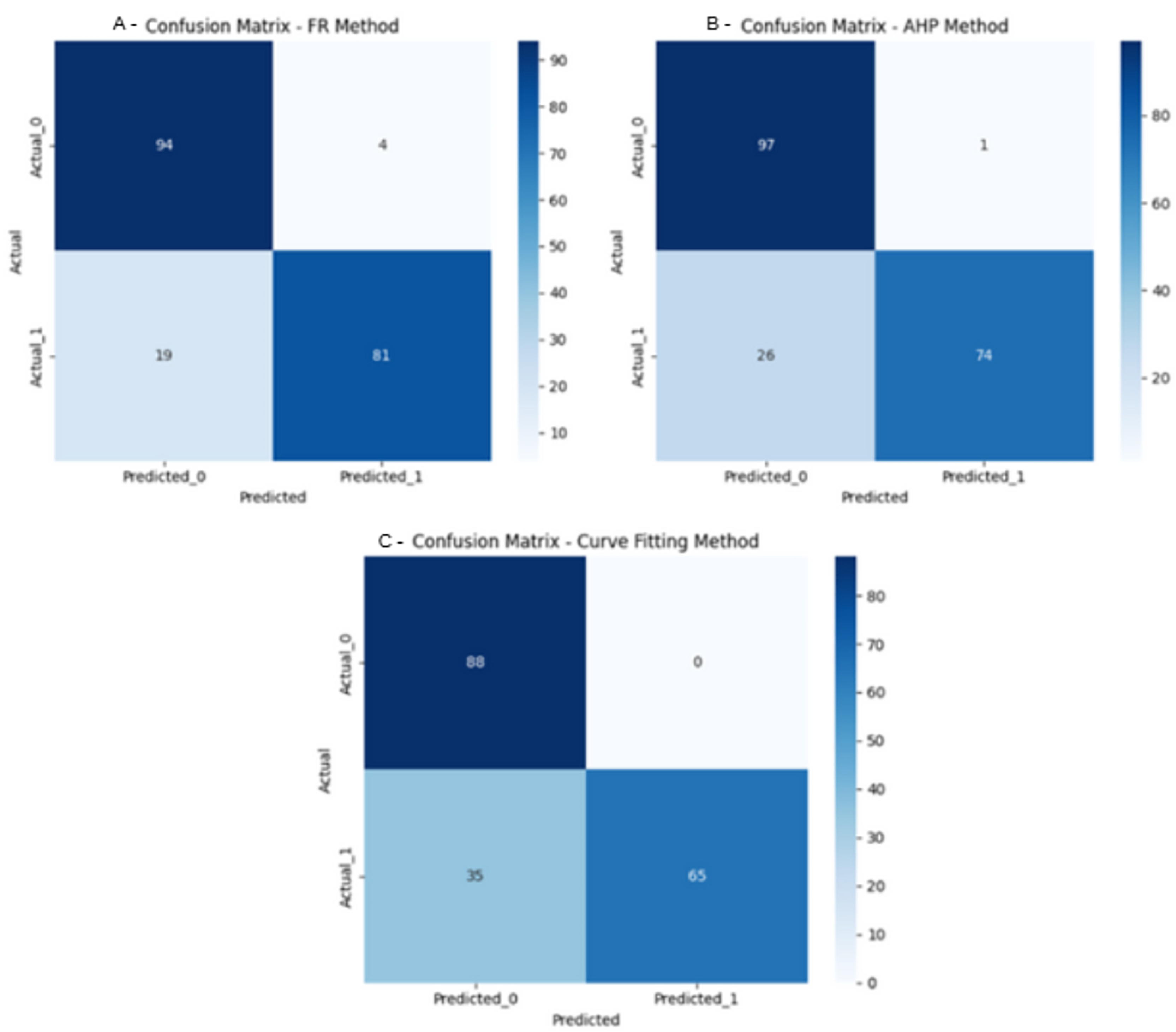
To evaluate model performance, landslide susceptibility outputs were validated using pixel count distributions from two groups: the landslide test group and the control group. Each entry in the table represents the frequency of pixel values assigned by the susceptibility models to areas known to be affected by landslides (test) or stable areas (control). These pixel counts were used as the input values to generate ROC curves and calculate F1-scores. Specifically, each model’s susceptibility scores were interpreted as continuous variables, and the optimal threshold for classification was determined by maximizing the F1-score. Based on this threshold, binary classification outputs were created and confusion matrices were generated for each method (Fig. 11). These matrices display the number of true positives (correctly predicted landslide pixels), false positives (non-landslide pixels misclassified as landslides), true negatives, and false negatives. The FR method achieved an F1-score of 0.876, while the AHP and Curve-Fitting methods followed closely, with F1-scores of 0.846 and 0.787 respectively. In addition, ROC curves were plotted to visualize model performance across thresholds, and AUC values were calculated (Fig. 12). The AUC scores, 0.88 (FR), 0.87 (AHP), and 0.79 (Curve Fitting), confirmed strong classification capability for all methods, with FR offering the best overall balance of detection and precision.
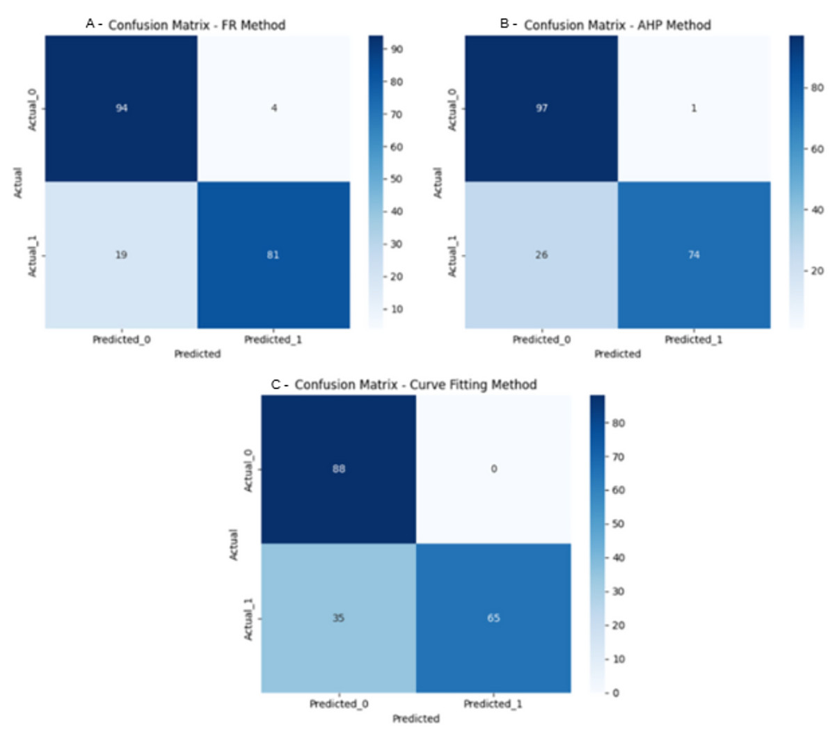
Figure 11: Confusion matrix of the methods.
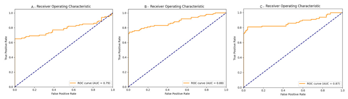
Figure 12: ROC curves and corresponding AUC values for the Frequency Ratio (FR), Analytical Hierarchy Process (AHP), and curve fitting methods.
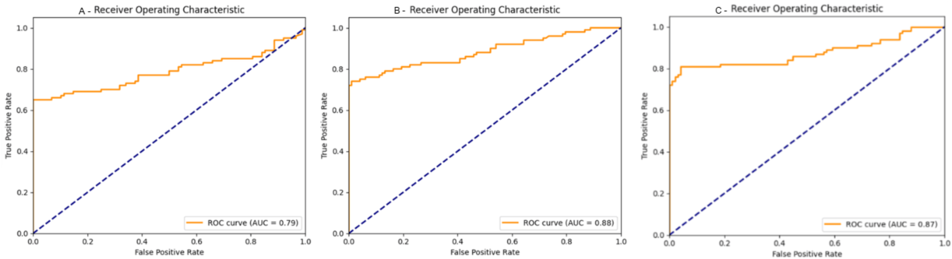
Discussion
A significant number of landslides have frequently occurred related to the climatic, topographic, and geological characteristics of the region. In the western part, the land cover is heavy forest, the river and road network are less dense, and the terrain slope is generally higher than in the eastern part. The low terrain slopes and dense river network have created areas suitable for agriculture and settlement in the eastern part. This topographic contrast creates varied slope stability conditions across the region, with steeper western slopes contributing to higher erosion and shallow landslide activity, while the gentler eastern slopes are more prone to water saturation and slow-moving failures. Human activities are also the main cause of catastrophic landslides in loess areas (Tyagi, Tiwari & James, 2022; Chowdhury et al., 2024). Excavation at the slope toe during engineering construction induces stress concentrations and uneven foundation settlement, destabilizing slopes. Urban expansion and the construction of supporting infrastructure alter the geomorphological, geological, and hydrological conditions of the area, triggering crustal stress changes and the development of landslide-prone structures. Linear infrastructure projects such as roads and pipelines, often built on river terraces, exacerbate these issues through slope cutting, long-term vibration, and repeated loading. These processes can re-activate dormant landslides (Tyagi, Tiwari & James, 2022). Furthermore, loess soils are highly sensitive to water and undergo significant softening under saturation. Agricultural irrigation leads to rising groundwater levels and altered hydrogeological structures, thereby increasing landslide likelihood (Chowdhury et al., 2024; Tyagi, Tiwari & James, 2022). In particular, the expansion of road networks and settlements has disturbed slope stability and increased erosion potential. Such anthropogenic influences have been widely recognized as secondary triggers for landslides in various geomorphological settings (Gorsevski, Gessler & Jankowski, 2003; Reichenbach et al., 2018). In our study, landslides were notably more frequent in areas with reduced forest density and proximity to roads, supporting the view that land cover modification plays a critical role in slope destabilization. It was observed that most of the landslides were developed in the areas covered by moderate forests and light forests, agriculture, and settlements. In the low altitudes, slope saturation by water might be higher because of the intense rainfall, changes in ground-water levels, and surface-water level changes along coastlines. Ayancık Member is also more favorable lithology for the landslide occurrences. Most of the landslides are located in this unit. It was observed that most of the landslides occurred in areas with convex and concave curvatures and between 0–500 m distance to the roads, rivers, and faults.
The spatial analysis outputs from the three methods support these observations. According to the FR method, the areas within 500 m of roads, with convex curvature, and those covered by the Ayancık Member, show the highest frequency ratio values. The AHP model similarly emphasized settlement zones, low altitudes (0–300 m), and proximity to rivers and faults as highly weighted. The Curve Fitting method highlighted the influence of Kusuri Formation, convex curvatures, slopes between 14°–21°, and proximity to rivers and faults, indicating strong predictive alignment with physical characteristics of known landslide locations.
Several regional studies have investigated landslide susceptibility in the Black Sea region using similar methods, providing a basis for comparison with our results. Akgün et al. (2012) indicated that many of the landslides between Sinop and Gerze occurred in the areas covered by the Sinop, Atbasi, and Akveren formations, having moderate vegetation, gentle slopes, and altitudes less than 954.95 m. Çellek, Bulut & Ersoy (2015) noted that the areas covered with Sinop, Atbasi, and Akveren formations, the slopes having E, NE, N, W, and NW aspects, and the areas that are close to the main roads between 0 and 250 m are the most favorable for landslide occurrence around Sinop. Işık, Doyuran & Ulusay (2004) studied a rotational coastal slide that occurred in 1988 within the settled area of the city of Sinop and caused extensive damage to buildings settled on the slope. The slide took place within the Saraycık formation consists of stiff clay. According to previous studies, the lithologic unit is not the region’s main triggering parameter for landslides. The landslides have occurred in any formation that is composed of sand and clay composition in the region. The elevation, curvature, terrain slope, proximity to the road and river parameters are prominent triggering factors for landslide occurrence in the studied area according to the applied methods.
In this study, the FR, and AHP methods reveal similar results to the previous studies. Most of the validation set landslides fall in moderate and high susceptible areas. The percentages of moderate (11.81%, 30.35%, 28.59%), high (36.57%, 26.64%, 33.48%), and very high (15.18%, 12.51%, 19.77%) susceptible classes calculated by the FR, AHP, and curve fitting methods show that the percentages of high and very high classes are higher than the results of previous studies conducted in the region. These values suggest that the Curve Fitting method identifies a higher proportion of very high- and high-susceptibility areas compared to the other methods, indicating its stronger spatial detection capability. Çellek, Bulut & Ersoy (2015) prepared the landslide susceptibility map of the area between Sinop and Gerze using the AHP method. They used lithology, aspect, slope, curvature, land-use, precipitation, and road, fault, and stream data as triggering factors. According to their susceptibility map, very low, low, moderate, high, and very high susceptibility classes covered 10.77%, 10.59%, 52.64%, 25.66%, and 0.34% of the map area, respectively. It was observed that the majority of validation set landslides were located in areas with moderate to high susceptibility. Okalp (2013) stated that the distribution of susceptibility zones in the landslide susceptibility map of the western Black Sea watershed area included Sinop City prepared from the AHP method is present at 23.13% in low, 12.39% in moderate, 18.46% in high, and 5.12% in very high class. Roccati et al. (2021) found that most of the landslides fall into high (35%) and very high (30%) susceptibility classes in the susceptibility map prepared by the AHP method for the Portofino promontory.
Ghorbanzadeh et al. (2022) stated that the F1-scores for the ResU-Net, OBIA, and combined ResU-Net–OBIA methods used for landslide susceptibility assessment in south Taiwan were 68.37, 54.59, and 76.56, respectively. Xu, Song & Hao (2022) indicated that the F1-scores for the Logistic Regression (LR), Random Forest (RF), DFCNN, and LSTM models were 0.58, 0.61, 0.62, and 0.61, respectively, when applied to evaluate landslide susceptibility in the Zigui-Badong area of the Three Gorges r area, China. The validation results of our three models (FR, AHP, and Curve Fitting) are summarized in Table 7, together with these recent studies, to provide a direct comparison. Compared to these studies, the Curve Fitting method used in our research identifies a higher percentage of very high and high susceptibility zones, suggesting it offers improved predictive coverage for the Sinop–Ayancık region.
| Study | Method (s) | Region | Reported metric (s) |
|---|---|---|---|
| This study (2025) | FR | Sinop–Ayancık, Türkiye | F1 = 0.876 |
| This study (2025) | AHP | Sinop–Ayancık, Türkiye | F1 = 0.846 |
| This study (2025) | Curve fitting | Sinop–Ayancık, Türkiye | F1 = 0.787 |
| Ghorbanzadeh et al. (2022) | ResU-Net, OBIA, ResU-Net+OBIA | South Taiwan | F1 = 68.37, 54.59, 76.56 |
| Xu, Song & Hao (2022) | LR, RF, DFCNN, LSTM | Zigui–Badong, China | F1 = 0.58–0.62 |
Limitations
Each method employed in this study has inherent limitations. The FR method relies on the assumption that past landslide occurrences accurately predict future events. However, this assumption may be disrupted by dynamic factors such as land use change, deforestation, or altered precipitation patterns due to climate change, which can shift susceptibility conditions over time.
The AHP method’s effectiveness is limited by subjective expert judgments, which may introduce biases or inconsistencies. However, applying pairwise consistency checks and performing sensitivity analysis can help reduce this bias and improve the robustness of the weighting process.
The Curve Fitting method is constrained by the chosen mathematical equation’s assumptions and is sensitive to the accuracy of input data and presence of outliers. This approach may have reduced predictive power when applied across different geographic or environmental contexts, limiting generalizability.
Conclusion
In this study, landslide susceptibility mapping was conducted using three well-established methods: FR, AHP, and Curve Fitting. These were used to evaluate and compare their prediction capabilities in the Sinop–Ayancık region of Türkiye. Each method produced reliable results, identifying critical risk areas based on spatial conditioning factors such as lithology, slope, curvature, and proximity to infrastructure. Among the methods, Curve Fitting demonstrated the highest landslide capture rate (81.84%) when moderate to very high susceptibility zones were considered. Although its F1-score (0.787) was lower than that of FR (0.876) and AHP (0.846), Curve Fitting’s ability to capture a broader distribution of potential landslide zones highlights its utility for spatial coverage. The FR method showed a balanced performance, achieving the highest F1-score and demonstrating strong precision and recall.
These results highlight that the choice of method can influence both the resolution and reliability of susceptibility predictions. For local authorities, planners, and risk managers, the susceptibility maps produced in this study can serve as a valuable tool for land-use planning, infrastructure development, and prioritization of mitigation strategies in vulnerable areas. The findings also underline the need to integrate multiple sources of data (geological, topographic, and anthropogenic) into susceptibility analysis to reflect real-world complexity.
Looking ahead, future studies should explore incorporating additional dynamic variables such as rainfall events, soil moisture, and time-series satellite data to reflect short-term triggers of landslides.
Supplemental Information
Pixel count distributions for the landslide test group and control group, extracted from susceptibility output maps produced by FR, AHP, and Curve Fitting methods.
These values were used as input for model validation, enabling the calculation of confusion matrices, F1-scores, and Receiver Operating Characteristic (ROC) curves. The counts reflect how each model classified known landslide and stable areas, providing the basis for AUC and threshold-based performance evaluation.