
MOD-YOLOv8: a new YOLOv8-based model for meniscal tear detection in knee MRI
- Published
- Accepted
- Received
- Academic Editor
- Ankit Vishnoi
- Subject Areas
- Algorithms and Analysis of Algorithms, Artificial Intelligence, Computer Vision, Data Mining and Machine Learning, Neural Networks
- Keywords
- Meniscal tear, Deep learning, Knee joint, Magnetic resonance imaging, Radiological, Artificial intelligence
- Copyright
- © 2026 Şimşek et al.
- Licence
- This is an open access article distributed under the terms of the Creative Commons Attribution License, which permits unrestricted use, distribution, reproduction and adaptation in any medium and for any purpose provided that it is properly attributed. For attribution, the original author(s), title, publication source (PeerJ Computer Science) and either DOI or URL of the article must be cited.
- Cite this article
- 2026. MOD-YOLOv8: a new YOLOv8-based model for meniscal tear detection in knee MRI. PeerJ Computer Science 12:e3530 https://doi.org/10.7717/peerj-cs.3530
Abstract
This study aimed to develop a deep learning–based approach for recognising meniscal tears on knee magnetic resonance imaging (MRI). A total of 600 examinations were randomly selected from the publicly available FastMRI dataset, yielding 828 labelled sagittal images for model development and evaluation. We proposed MOD-YOLOv8, an adaptation of the You Only Look Once version 8 (YOLOv8) architecture. Its performance was benchmarked against state-of-the-art (SOTA) YOLO models (YOLOv5, YOLOv6, YOLOv8, and YOLOv9t) using five-fold cross-validation and was also compared with RT-DETR and Detectron2 under the same dataset and evaluation protocol. The final metrics for the proposed model, including precision (P), recall (R), mAP50, and F1-score, were 0.8450, 0.8902, 0.9227, and 0.8670, respectively. Confidence intervals for P, R, mAP50, and F1-score were 0.8738 (95% CI [0.8020–0.9456]), 0.8846 (95% CI [0.8652–0.9041]), 0.8966 (95% CI [0.8507–0.9424]), and 0.8512 (95% CI [0.7995–0.9029]), respectively. These results demonstrate that MOD-YOLOv8 consistently outperforms the compared baselines while providing reliable detection performance. Heatmap-based visualisation indicated that the model focused on clinically relevant tear regions, supporting interpretability. Overall, MOD-YOLOv8 demonstrates superior accuracy, reliability, and potential clinical applicability for detecting meniscal tears on MRI.
Introduction
Meniscus tissue consists of two crescent-shaped, C-shaped fibrocartilage structures located between the femur and tibia bones. The tibial side features a flat surface, while the femoral side has a concave surface. Their main functions are to facilitate movement and to absorb shock. The fibrocartilage of the meniscus contains small amounts of water and fat. Water makes up approximately 65–72% of the meniscus, collagen 20–25%, and proteoglycans less than 1%. The water content is highest in the posterior horns of the menisci compared to their central or anterior parts (Mameri et al., 2022). In the coronal section, the anterior and posterior horns of the meniscus, as well as the meniscal root structure, are visible; in the sagittal section, it appears as a triangular, bowtie-shaped structure (Kocabey et al., 2004; Englund et al., 2012).
The meniscus can be injured in traumatic situations and can be seen as partial or complex tears, depending on the type of trauma (D’Ambrosi et al., 2024). Detecting meniscal tears is crucial due to their negative impact on patients’ quality of life, gait, and locking symptoms. Positive examination tests are often used in these cases.
Magnetic resonance imaging (MRI) is the primary method for detecting meniscal injuries due to its high spatial and contrast resolution, which accurately represents the high-water content and collagenous structure of meniscal tissue. MRI sequences, such as T1-weighted imaging, T2-WI, fat-suppressed T1-WI, and proton density series, reveal fibrocartilaginous structures. Recently, artificial intelligence (AI) methods have begun to be incorporated into routine practice, complementing radiological applications and human factors in the detection of pathologies, and these current AI tools play a crucial role.
Deep Learning (DL) is a subfield of AI that has experienced rapid development in recent years. With the advancement of technology, the use of these algorithms in medicine has led to significant changes in many fields. Large data sets of patients have started to be used with AI algorithms, resulting in improvements in many areas, including early diagnosis of diseases, structuring treatment plans, and diagnosing diseases (Kaur et al., 2020). DL algorithms, especially convolutional neural networks (CNNs), have rapidly become the preferred methodology for analyzing radiological images (Litjens et al., 2017). For example, DL technologies are used for breast cancer tumor detection (Mahoro & Akhloufi, 2022), brain tumor detection (Arabahmadi, Farahbakhsh & Rezazadeh, 2022), lung disease detection (Jasmine Pemeena Priyadarsini et al., 2023), diagnosis of developmental dysplasia of the hip (Mendi, Batur & Çay, 2022), fracture detection (Ju & Cai, 2023) based on radiological findings.
DL algorithms can improve the diagnostic performance of radiologists and further support clinical workflows through collaboration between radiologists, engineers and data scientists (Rizk et al., 2021). In this context, several studies in the literature have focused on the detection of meniscal tears using MRI. Bien et al. (2018) proposed a convolutional neural network (CNN)-based DL model that simultaneously utilised coronal, sagittal and axial MRI slices to detect both general abnormalities and specific diagnoses, such as anterior cruciate ligament and meniscal tears. Couteaux et al. (2019) used a region-based CNN (R-CNN) algorithm on sagittal slices to detect and classify meniscal tears, while Roblot et al. (2019) developed a CNN-based algorithm to detect and characterise meniscal tears in sagittal MRI images. Similarly, Fritz et al. (2020) presented a deep convolutional neural network (DCNN)-based model for the detection of meniscal tears in sagittal and coronal MRI images and validated it against clinical findings. Rizk et al. (2021) also proposed a CNN-based method for detecting and characterizing meniscal lesions from sagittal and coronal slices of adult knee MRI images.
In addition to the classical CNN approaches, more advanced and hybrid CNN-based models were also presented. Hung et al. (2023) integrated the Darknet-53 architecture into the You Only Look Once version 4 (YOLOv4) algorithm to analyse coronal and sagittal slices. Ma et al. (2023) developed a novel C-PCNN neural network for meniscal injury diagnosis and showed that sagittal slices provide richer information for damage detection. Chou et al. (2023) designed an AI model incorporating arthroscopic findings, using Scaled-YOLOv4 to detect meniscal position and EfficientNet-B7 to detect meniscal tears, for both sagittal and coronal slices. Harman et al. (2023) investigated the use of accelerated MRI and nDetection to detect meniscal tears.
More recent studies have presented even more advanced methods. Ying et al. (2024) developed a DL framework based on knowledge distillation, combining MRI and arthroscopy data. In their work, a residual network (ResNet)-18-based multimodal teacher network was utilized to train an MRI-only learner network, resulting in improved detection accuracy for medial and lateral meniscal tears. Güngör et al. (2025) showed that advanced CNN models such as YOLOv8 and EfficientNetV2 can accurately classify meniscal tears even on relatively small datasets and proposed a two-stage system for localisation and classification of meniscal tears. Tanwar et al. (2025) presented MV2SwinNet, a hybrid model that integrates the architectures of MobileNetV2 and Swin Transformer and effectively combines local and global features to achieve high diagnostic accuracy.
Transformer-based approaches have also gained importance in this area. Genç et al. (2025) combined a Vision Transformer (ViT)-based DL method with ElasticNet for feature reduction and support vector machine (SVM) for classification and achieved high accuracy on 1,499 MRI scans. Similarly, Vaishnavi Reddy et al. (2025) developed a model based on Mask R-CNN to differentiate normal from abnormal medial menisci on MRI. Using 3,600 sagittal PD-FS MRI images from 800 patients, their model showed high accuracy at the pixel level.
Overall, these studies demonstrate that state-of-the-art (SOTA) models can achieve high performance in detecting meniscal tears, even with limited datasets, and illustrate the potential of automated diagnostic systems that can be quickly integrated into clinical practice.
Various CNN, R-CNN, YOLO, and transformer-based approaches for detecting meniscal tears using MRI have been applied in the literature. These models have shown promising results. However, most studies either relied on earlier versions of YOLO, limited their analysis to a single image plane, or lacked a systematic comparison with a broader range of SOTA architectures. Additionally, several studies have explicitly incorporated the interpretability of the model to support clinical decision-making. Despite advances in the field, a clear research gap remains in the development and validation of a lightweight yet highly accurate YOLOv8-based architecture designed explicitly for meniscal tear detection using MRI.
To fill this gap, the current study presents MOD-YOLOv8, an extended variant of YOLOv8 with additional optimised layers for improved feature extraction and detection performance. Furthermore, the interpretability of the model has been enhanced by heatmap visualizations that provide clinicians with insight into the algorithm’s decision-making process. Thus, this study not only improves the technical performance of meniscal tear detection models but also increases their clinical applicability. The features of this work can be listed as follows:
The MOD-YOLOv8 model was developed for the detection of meniscal tears using DL methods.
A set of optimized layers is added to the MOD-YOLOv8 model.
The performance of the MOD-YOLOv8 model was compared with other widely used models of the YOLO series.
Our research illustrates the effectiveness of deep learning-based methods for detecting meniscus tears. In various relevant fields (orthopedics and traumatology, Physical Therapy and Rehabilitation (PTR), emergency, etc.), the model facilitates the simpler identification of meniscal tears, particularly in radiological diagnostics. It may also expedite the diagnosis and treatment procedures. By demonstrating how DL approaches can be successfully applied and YOLO-based models optimized in a crucial clinical application area, such as meniscal tear detection, this study adds scientific value to the literature.
Materials and Methods
Ethical approval and consent to participate
The Ethics Committee approved this retrospective randomized study for Non-Interventional Clinical Research of Tekirdağ Namık Kemal University (research protocol number: 2024.02.01.02, date: 04.04.2024). The data used in this study were obtained from the publicly available FastMRI dataset (https://fastmri.med.nyu.edu) (Zbontar et al., 2018; Knoll et al., 2020) provided by NYU Langone Health. The creation of the FastMRI dataset was part of a study, the organization of which was approved by NYU Langone Health’s local institutional review boards. Therefore, participant consent was not required in our study. The dataset was de-identified using standardized tools such as the Radiological Society of North America’s Clinical Trial Processor to ensure that no protected health information was left behind. The dataset was created as part of a study approved by the NYU Langone Health Institutional Review Board (IRB). No additional consent was required for participation, as data were anonymized before release and used in accordance with NYU Langone Health’s ethical guidelines.
Patient population and selection
The data used in the preparation of this article were obtained from the New York University (NYU) FastMRI Initiative database (fastmri.med.nyu.edu). The FastMRI Dataset is considered proprietary to New York University and NYU Langone Health (together “NYU”) (Zbontar et al., 2018; Knoll et al., 2020). The FastMRI dataset includes k-space data. It also contains 10,012 sequential DICOM (Digital Imaging and Communications in Medicine) image data from 9,290 patients undergoing clinical knee MRI examinations, and is a full complement of represented clinical acquisitions, including various tissue contrasts and different imaging planes (Knoll et al., 2020).
From the FastMRI dataset, radiological images of 600 patients were randomly selected. After applying inclusion and exclusion criteria, images from 471 patients were included in the study (Fig. 1) (Şimşek et al., 2025). The age range of the selected patients was 2–85 years, with a mean age of 47.79 years. Of the 471 patients, 44.48% (n = 210) were female, 42.02% (n = 198) were male, and 13.38% (n = 63) were classified as other gender. MRI images of the right knee were used for 53.08% (n = 250) and MRI images of the left knee for 46.92% (n = 221). While 16.35% (n = 77) of patients had no meniscal tear, 83.65% (n = 394) had meniscal tears. In the group with meniscal tears, 53.81% (n = 212) were on the right side and 46.19% (n = 182) on the left side. Most tears were located on the medial meniscus (67.51%, n = 266) and fewer on the lateral meniscus (32.49%, n = 128). The most common tear site was the posterior horn (66.00%, n = 260), followed by the medial (11.77%, n = 70), anterior (14.97%, n = 59), and root regions (1.26%, n = 5). Regarding the type of tear, the most common was horizontal (42.63%, n = 168), followed by horizontal-oblique (33.50%, n = 132), vertical (9.33%, n = 37), oblique (7.36%, n = 29), horizontal-vertical (6.09%, n = 24), and vertical-oblique (1.02%, n = 4).
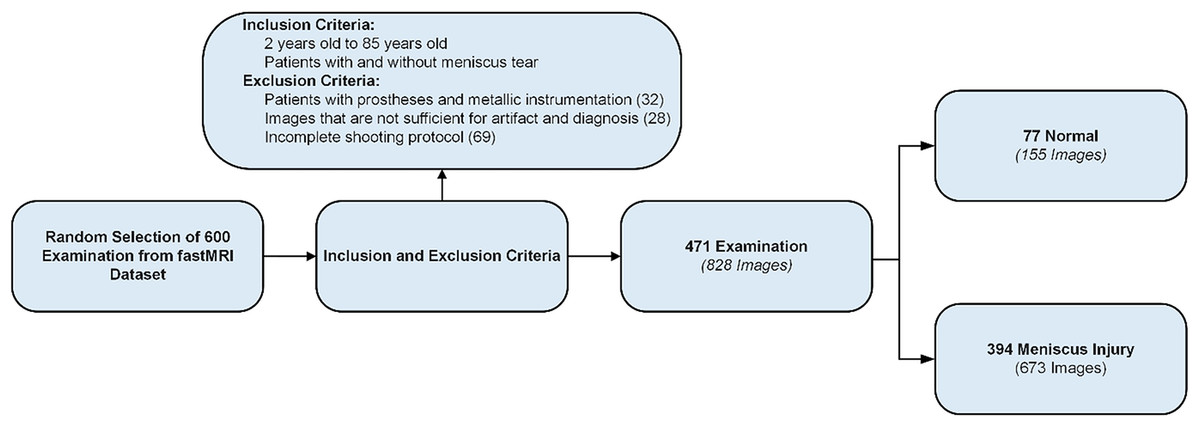
Figure 1: Data set creation process.
Selection and evaluation of images
The DICOM-formatted data of the patients were categorized and labeled based on the pulse sequences. Specifically, 505 T2-weighted and 323 PD-weighted images of 828 images were randomly selected from the dataset. Images were also categorized according to the presence or absence of a meniscal tear.
The image selection, categorization, and labeling process was performed by a radiologist with expertise in radiology (12 years) and an expert in orthopedics and traumatology (12 years). Two computer engineers (8 and 15 years) were also involved in the labeling of the data.
Only sagittal MRI slices that provided optimal visualisation of meniscal tears were included in the study (Ma et al., 2023). This approach was adopted to enhance diagnostic accuracy and optimize the model’s performance.
Scanning protocol
FOV 140 × 140 mm2, matrix size 320 × 320 pixels, turbo factor 4, slice thickness 3 mm, TR 2,750–3,000 ms, TE 27–32 ms, receive coil 15 channel (Knoll et al., 2020).
Data set and annotation
The study employed a dataset comprised of radiologic images from 471 patients. After applying the exclusion criteria, an average of 1.7 images per patient was obtained, resulting in a total of 828 image samples used to create the dataset (Fig. 1). Images were extracted in Portable Network Graphics (PNG) format. To provide a reliable reference for training our model, bounding boxes normalized to the range [0, 1] were placed around the medial and lateral menisci in each image. The images in this sagittal slice were then labeled as either “tear” or “no_tear”.
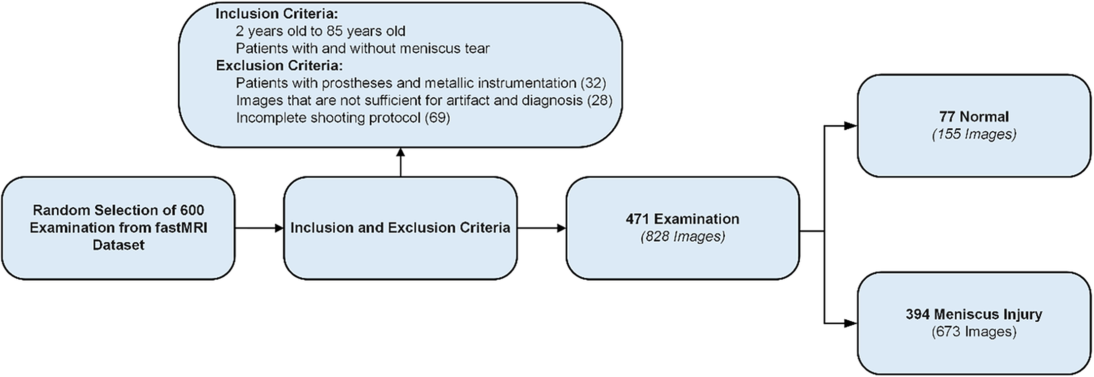
Of the 828 images in the dataset, 147 images are non_tear images, and 681 images are tear images. The imbalance in the dataset is due to the general use of the FastMRI dataset, which is more commonly used in clinical examinations for tear detection and detection of various abnormalities, with limited access to images of healthy patients. In the image with a meniscal tear, only the area around the torn meniscus is labeled. In the image of a healthy patient without a tear, both the lateral meniscus and the medial meniscus are labeled. There were 681 labelings on 681 images with tears and 260 labelings on 147 images without tears. Thus, a more balanced dataset was created for detecting meniscal tears. Figure 2 shows the labeled images used in the dataset. The online tool RoboFlow (Dwyer et al., 2025) was used for processes such as labeling the images, sizing the data set and splitting.
Figure 2: Labeled MRI images used in the dataset.
(A) Sagittal section, tear on the anterior side of the lateral meniscus. (B, C) Sagittal section, meniscus without tear.
Pre-processing of the images
Since the MRI images obtained have different resolutions, they were preprocessed to match the input dimensions of the YOLO algorithm (640 × 640 px). This process was carried out with RoboFlow.
YOLOV8 algorithm
You Only Look Once (YOLO) is a fast and efficient DL algorithm for object detection. YOLOv8, one of the versions of the YOLO family released by Ultralytics in 2023, includes five different scaled versions: YOLOv8n (nano), YOLOv8s (small), YOLOv8m (medium), YOLOv8l (large), and YOLOv8x (extra-large). YOLOv8 supports multi-view tasks such as object detection, segmentation, pose estimation, tracking, and classification (Terven, Córdova-Esparza & Romero-González, 2023; Sohan, Sai Ram & Rami Reddy, 2024).
YOLOv8 employs a similar backbone to YOLOv5, with modifications to the CSPLayer, specifically the C2f module. The YOLOv8 architecture comprises three main networks: the backbone, neck, and head, all of which utilize convolutional neural networks.
The backbone consists of multiple convolutional layers arranged in a sequential manner that extract relevant features from the input image. The new C2f module integrates high-level features with contextual information to improve detection accuracy. The head takes the feature maps produced by the backbone and processes the final output of the model into bounding boxes and object classes (Terven, Córdova-Esparza & Romero-González, 2023; Sohan, Sai Ram & Rami Reddy, 2024).
MOD-YOLOV8 architecture
In this study, we present the MOD-YOLOv8 model built on the YOLOv8 architecture (Jocher, Qiu & Chaurasia, 2023) to accurately diagnose meniscal tears and their localization. It is seen that new model approaches have been created by modifying the YOLOv8 architecture for solving different problems (Zhang, 2023; Ju & Cai, 2023; Zhao et al., 2024b). The YOLOv8 architecture inspires our MOD-YOLOv8 model architecture and includes some new layers and improvements in the backbone and head networks (Fig. 3).
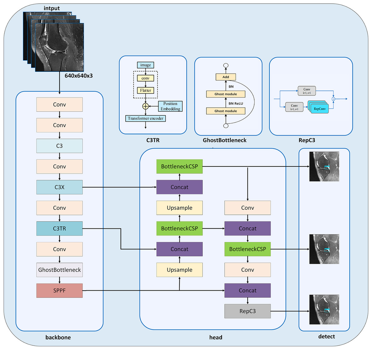
Figure 3: MOD-YOLOv8 architecture.
In the MOD-YOLOv8 model, the Conv module is used for basic feature extraction, similar to YOLOv8. The modules C3 (CSP Bottleneck with three convolutions), C3x (C3 module with cross-convolutions), and C3TR (C3 module with TransformerBlock) offer additional depth and feature extraction capabilities not available in YOLOv8. In particular, the C3 module helps the model learn more complex features. To enhance the network’s depth and improve its feature extraction capabilities, the C3 module was added to the backbone network (Park et al., 2018; Sun, Feng & Chen, 2024). The C3 module, which was added instead of the C2f module, contains more bottlenecks. C3 increases the ability to learn from input images through multi-layer processing in the MOD-YOLOv8 architecture. The C3x module contains structural components, like the C3 layer, and additionally utilizes cross-convolutions. The C3x module has been used to learn various features and enhance the model’s performance. The transformer architecture was integrated into the C3 module to create the C3TR module. By replacing the bottleneck module in the C3 module, richer image information can be extracted. The transformer block serves as the core component in the C3TR framework, which adopts the classic transformer encoder architecture (Lv & Su, 2024). Thanks to the transformer module and the multi-attention mechanism in the C3TR module, multi-scale information can be extracted, allowing for a focus on both location and feature information.
The GhostBottleneck module achieves similar performance using fewer parameters. This module aims to enhance performance while maintaining the lightweight nature of the developed model. The GhostBottleneck module is added to the backbone network to reduce the overall size of the model without increasing the network parameters, to enable the network to better and faster understand redundant information, and to improve the accuracy of the model (Zhao et al., 2021).
The BottleneckCSP module is mainly used in the head network to extract deep semantic information from images, enrich semantic information, and combine feature maps at different scales (Li, Wang & Zhang, 2023). The BottleneckCSP and RepC3 modules are utilized in the MOD-YOLOv8 architecture to estimate small targets and learn low- and high-level information effectively, especially in the small pixel areas of the input images. SPFF, Concat and Upsample modules are also included in the YOLOv8 architecture.
Evaluation metrics
Various metrics such as recall (R), precision (P), average precision (AP), mean average precision (mAP) and F1-score were used to evaluate the performance of the MOD-YOLOv8 model and the results of comparisons with other models. The F1-score is a combined measure of P and R values. AP and mAP are measures of model recognition accuracy. mAP50 and AP50 metrics are included in this study. The most common metrics used to evaluate models are R, P, AP, mAP, and F1-score, which are expressed in Eqs. (1)–(5), respectively.
(1)
(2)
(3)
(4)
(5)
For Eqs. (1) and (2): TP indicates true positives, FN indicates false negatives, and FP indicates false positives. The models were also evaluated in terms of FLOPs, number of parameters, and training times. FLOPs (Floating-Point Operations Per Second) are a measure of computer hardware performance and algorithm complexity. Parameters are numerical values that the model learns from the data and uses to make predictions.
Experiment setup and hyperparameters
All experiments were performed using Google Colab. Google Colab is a notebook where Google servers perform high computations. For the analysis of the dataset, the Ultralytics YOLOv8.2.38 library, torch-2.3.0+cu121, and Python 3.10.12 programming language were used on the Google Colab platform, running on an NVIDIA A100 GPU (SXM4-40GB, 40514MiB) processing unit.
After repeated experiments, the final hyperparameters were set as in Table 1, and all set hyperparameters remained unchanged in the final training. To expedite the process, we initially created a reduced subset of the dataset. We conducted a manual random grid search, testing various combinations of key parameters, including learning rate, dynamics, and stack size. On each trial, the model’s performance was evaluated and compared using standard metrics. This iterative procedure—essentially repeated experiments with manually selected parameter values—enabled us to determine efficient hyperparameter settings in less time, without relying on automatic hyperparameter optimization algorithms. When setting hyperparameters manually, the trade-off between convergence speed and model stability, as well as selecting a suitable batch size, poses a significant challenge. Higher learning rates occasionally led to drift, while lower rates significantly slowed down convergence.
| Hyperparameter | Description |
|---|---|
| Workers | 2 |
| Batch | 12 |
| Device | 0 |
| Epochs | 100 |
| lr0 | 0.0100 |
| lrf | 0.0100 |
| Momentum | 0.9500 |
| Weight_decay | 0.0001 |
| Warmup_epochs | 10 |
| Warmup_momentum | 0.5000 |
| Warmup_bias_lr | 0.1000 |
| Optimizer | SGD |
Note:
lr0, Initial learning; lrf, final learning rate.
HiResCAM for heatmap
Heatmaps are used to provide a more detailed and visual analysis of the DL model’s decision-making processes and the accuracy of its detection. HiResCAM was used to determine which regions in the input image influence the model’s decision-making process. HiResCAM (Draelos & Carin, 2020) was introduced in 2020 as an alternative to GradCAM. In contrast to GradCAM, which relies on gradient backpropagation to weight activation maps, HiResCAM directly uses the forward activations of feature maps to calculate class-specific contributions. This enables HiResCAM to generate more accurate and higher-resolution saliency maps, thereby avoiding gradient-induced noise or distortion. As a result, HiResCAM provides a clearer localisation of the most relevant regions and offers a more accurate explanation of the model decision compared to GradCAM and similar gradient-based methods (Draelos & Carin, 2020; Rheude et al., 2024; Rafati et al., 2025).
Results
The MOD-YOLOv8 architecture for meniscal tear detection is compared to other YOLO series, with transfer learning not used. Initial unweighted training was performed over 100 epochs, with input images configured at 640 × 640 px and a batch size of 12. The models’ performance, practical application success, and generalization ability are compared. The best and last values of the metric values in the training of the models are given comparatively in Table 2 (demonstrating the metric performance indicators that were determined after completion of the model training).
| Models | PLast | PBest | RLast | RBest | mAP50Last | mAP50Best | F1-scoreLast | F1-scoreBest |
|---|---|---|---|---|---|---|---|---|
| YOLOv5 | 0.7849 | 0.8257 | 0.8563 | 0.8636 | 0.8609 | 0.8764 | 0.8191 | 0.8442 |
| YOLOv6 | 0.8528 | 0.8800 | 0.8718 | 0.9001 | 0.9048 | 0.9096 | 0.8622 | 0.8899 |
| YOLOv8 | 0.8601 | 0.8782 | 0.8426 | 0.8875 | 0.9032 | 0.9098 | 0.8513 | 0.8829 |
| YOLOv9t | 0.8420 | 0.8718 | 0.8488 | 0.8805 | 0.9013 | 0.9063 | 0.8454 | 0.8762 |
| MOD-YOLOv8 | 0.8450 | 0.9157 | 0.8902 | 0.9038 | 0.9227 | 0.9258 | 0.8671 | 0.9097 |
Note:
P, precision; R, recall; mAP, mean average precision. Bold values indicate the best results obtained among all conditions or methods analysed for the respective metric.
The best values represent the highest model performance achieved by the models during the training period, while the last values represent the performance at the end of 100 epochs. Compared to the other models, MOD-YOLOv8 achieved the best R, mAP50, and F1-scores, except for PLast. Although the MOD-YOLOv8 model achieved the highest PBest value (0.9157), its PLast value dropped to 0.8450 by the end of training. This relatively large gap indicates that precision is more susceptible to fluctuations compared to the other metrics. These fluctuations are clearly visible in Fig. 4A and are further explained in the following section. In contrast, the minor differences between the best and last values of R, mAP50, and F1 indicate that the model remained stable on these metrics throughout the training process. Overall, the MOD-YOLOv8 model performs better than the other models in detecting meniscus tears when considering P, R, mAP50, and F1-score together.
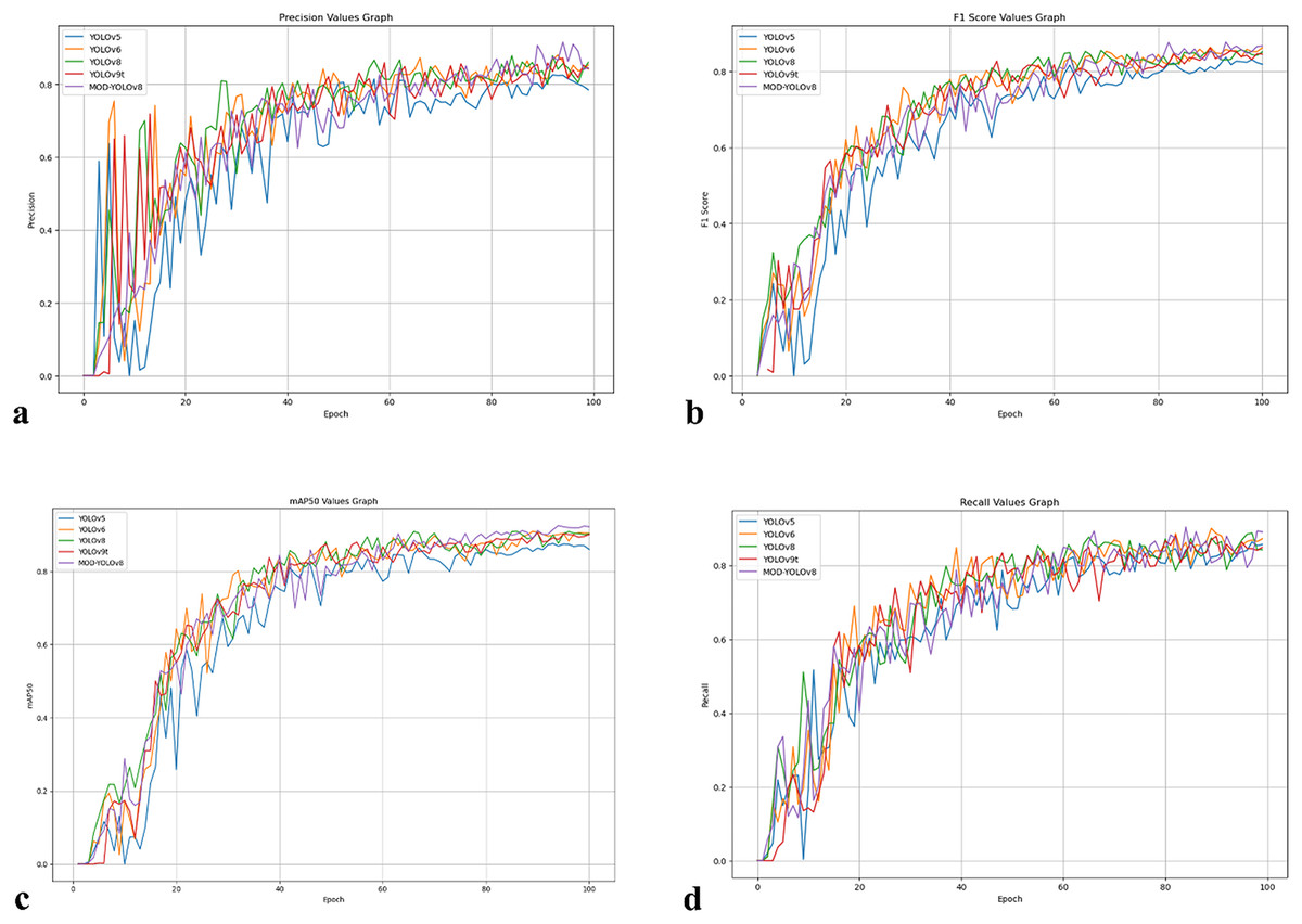
Figure 4: Curves showing P, R, mAP50 and F1-score values of the models over 100 epochs.
(A) P values curve. (B) R values curve. (C) mAP50 values curve, (D) F1-score values curve.
Figure 4 summarises the development of the metrics over 100 epochs. P (Fig. 4A) fluctuates more in the first epochs, consistent with the asymmetry of the dataset in terms of classes and annotations, and increases the early false positives. As training progresses, P stabilizes, and both YOLOv8 and MOD-YOLOv8 quickly reach high P values. The F1-score (Fig. 4B), which balances precision and recall, shows a more even convergence; YOLOv5 yields the lowest F1-score, while MOD-YOLOv8 achieves the best balance. mAP50 (Fig. 4C), which reflects the overall quality of recognition, improves and stabilises for all models, with MOD-YOLOv8 showing the strongest curve. R (Fig. 4D) increases more evenly; although YOLOv8 increases rapidly, MOD-YOLOv8 achieves the best final R. For all metrics, the curves stabilise after 60 epochs, with MOD-YOLOv8 consistently performing better than the alternatives overall.
Looking at Fig. 4 and Table 2, fluctuations can be observed in the initial phase, especially in the precision curves; after about 60 epochs, mAP50, R and F1-scores show a stable plateau. For MOD-YOLOv8, the P values are PBest 0.9157, PLast 0.8450; however, the differences in R (PBest and PLast: 0.9038, 0.8902) and mAP50 (PBest and PLast: 0.9258, 0.9227) are minor. This can be attributed to the fact that precision is more sensitive to factors such as class imbalance, small target size, and threshold sensitivity. Early stopping was not applied to equalise the training lengths for all models. To mitigate the impact of epoch-based randomness, the average of the last 10 epochs was calculated, yielding an average precision of 0.8727. In addition, as shown in Fig. 5, the precision curve was smoothed by applying the Exponential Moving Average (EMA), resulting in a more stable trend. These adjustments make the performance evaluation of MOD-YOLOv8 more reliable and reveal the generalisation behaviour of the model more clearly.
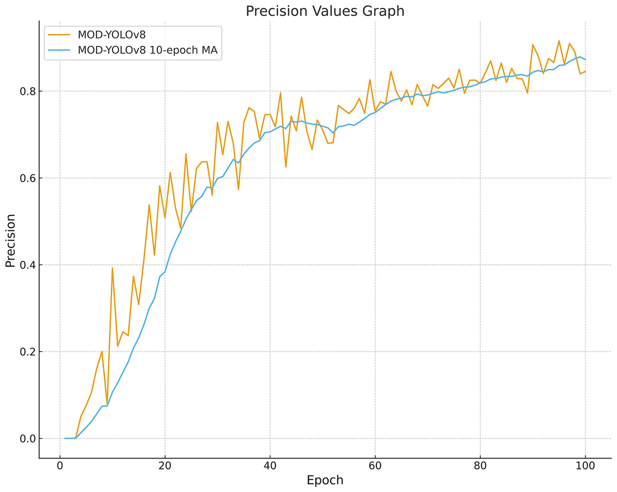
Figure 5: Precision curve smoothed with MOD-YOLOv8 and a 10-epoch moving average.
Following model optimization during the training phase, Table 3 displays the number of parameters, training duration, and GFLOPs. The YOLOv6 model has the highest number of parameters (~4.23M) and FLOPs/G (11.8), but it has the shortest training time of 12 min and 50 s. These values show the computational efficiency of the model. The YOLOv9t model has the lowest number of parameters (~2.00 M) and a FLOPs/G value of 7.6, but mAP50 has the longest training time of 19 min 23 s. The results show inefficiency and increasing complexity for this problem. MOD-YOLOv8, built on the YOLOv8 architecture, exhibits higher performance due to the modules used and has approximately 5% fewer parameters. The YOLOv8 and MOD-YOLOv8 models strike a balance between the number of parameters and computational complexity, with training times of 12 min 54 s and 13 min 5 s, respectively.
| Models | Parameters/M | FLOPs/G | Time/min |
|---|---|---|---|
| YOLOv5 | ~2.5000 M | 7.1000 | 12:58 |
| YOLOv6 | ~4.2300 M | 11.8000 | 12:50 |
| YOLOv8 | ~3.0100 M | 8.1000 | 12:54 |
| YOLOv9t | ~2.0000 M | 7.6000 | 19:23 |
| MOD-YOLOv8 | ~2.8600 M | 7.1000 | 13:05 |
Note:
M, Million; G, Giga. Bold values indicate the best results obtained among all conditions or methods analysed for the respective metric.
The dataset was labeled into two classes, according to the presence or absence of a tear (tear, no_tear). The performance of the models on each class is more accurately shown in Table 4, which shows the results of the validation series. To detect the meniscus region in the input images and classify whether a tear is present or not, P and AP50 metrics were analyzed, and MOD-YOLOv8 yielded the best results in this field. For the R metric, YOLOv5 demonstrates higher performance in determining whether a tear is present, while YOLOv9t shows higher performance in deciding whether a tear is present. The AP metric of the training is a metric that summarizes the accuracy and sensitivity performance of the model for an object class. The MOD-YOLOv8 model stands out as the most suitable model for object detection tasks, achieving the highest mAP50 and accuracy values of 0.8820 and 0.9630 in the AP50tear and AP50no_tear classes, respectively.
| Model | Class | P | R | AP50 |
|---|---|---|---|---|
| YOLOv5 | No_tear | 0.8200 | 0.9610 | 0.9460 |
| Tear | 0.7820 | 0.7660 | 0.7960 | |
| YOLOv6 | No_tear | 0.8950 | 0.9220 | 0.9460 |
| Tear | 0.8060 | 0.7880 | 0.8500 | |
| YOLOv8 | No_tear | 0.8710 | 0.8630 | 0.9380 |
| Tear | 0.8240 | 0.7860 | 0.8410 | |
| YOLOv9t | No_tear | 0.8520 | 0.9020 | 0.9430 |
| Tear | 0.8330 | 0.8030 | 0.8590 | |
| MOD-YOLOv8 | No_tear | 0.9490 | 0.8630 | 0.9630 |
| Tear | 0.8760 | 0.7880 | 0.8820 |
Note:
P, precision; R, recall; AP, average precision. Bold values indicate the best results obtained among all conditions or methods analysed for the respective metric.
K-fold cross-validation was employed to prevent overfitting of the MOD-YOLOv8 model (Bradshaw et al., 2023) and to align it with real-world applications better. K-fold validation divides the dataset into k parts, using one part as validation data and the remaining k − 1 parts as training data. In this study, k = 5. The 828 (941 labeling) sagittal slice images in the dataset were divided into five sections labeled K1, K2, K3, K4, and K5. This was done randomly by maintaining the ratio of torn images to non-torn images in each section at a constant level. Sections K2, K3, K4, and K5 were used to train, section K1 was used for validation, and the Fold1 model was obtained. This process was performed separately for Fold 2, Fold 3, Fold 4, and Fold 5. In this manner, five partitions were utilized as validation sets, and the confusion matrices for the five evaluations are presented in Fig. 6.
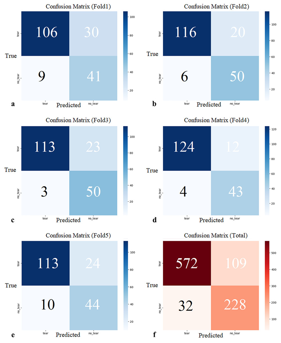
Figure 6: (A–E) Confusion matrices of each cross-validation and (F) total Confusion matrix of five-fold cross-validation.
The five-fold cross-validation showed that the proposed model generally predicted both classes (tear, no_tear) with satisfactory accuracy. The rate of correct predictions for the no_tear class was higher, while the performance for the tear class was relatively lower, but still acceptable. These results demonstrate the overall accuracy and consistency of the model, suggesting that it has the potential to be generalized to real data. Confidence intervals for precision, recall, mAP50, and F1-score were 0.8738 (95% CI [0.8020–0.9456]), 0.8846 (95% CI [0.8652–0.9041]), 0.8966 (95% CI [0.8507–0.9424]), and 0.8512 (95% CI [0.7995–0.9029]), respectively.
Figures 7A–7E shows the PR (precision-recall) curves for the individual folds together with the class-wise AP50 values. Across the five folds, the values for tear AP50 were 0.8130, 0.8890, 0.8520, 0.8410, and 0.8590, while the values for no_tear AP50 were 0.8710, 0.9740, 0.8980, 0.9100, and 0.9840, respectively. On average, tear scored 0.8508 (95% CI [0.8165–0.8851]) and no_tear scored 0.9274 (95% CI [0.8662–0.9886]). The absolute gap (no_tear, tear) across folds was 0.0766 (95% CI [0.0386–0.1146]), which corresponds to a relative decrease for the tear class of 0.0816 (95% CI [0.0460–0.1171])—i.e., 8.1588% (95% CI [4.6046–11.7131%]). In contrast, overall performance across all classes (mAP50) remained high with an average score of 0.8916 (95% CI [0.8415–0.9417]). These results quantify the imbalance of the PR curves, showing that while the overall performance is satisfactory, the tear class is the primary cause of performance loss.
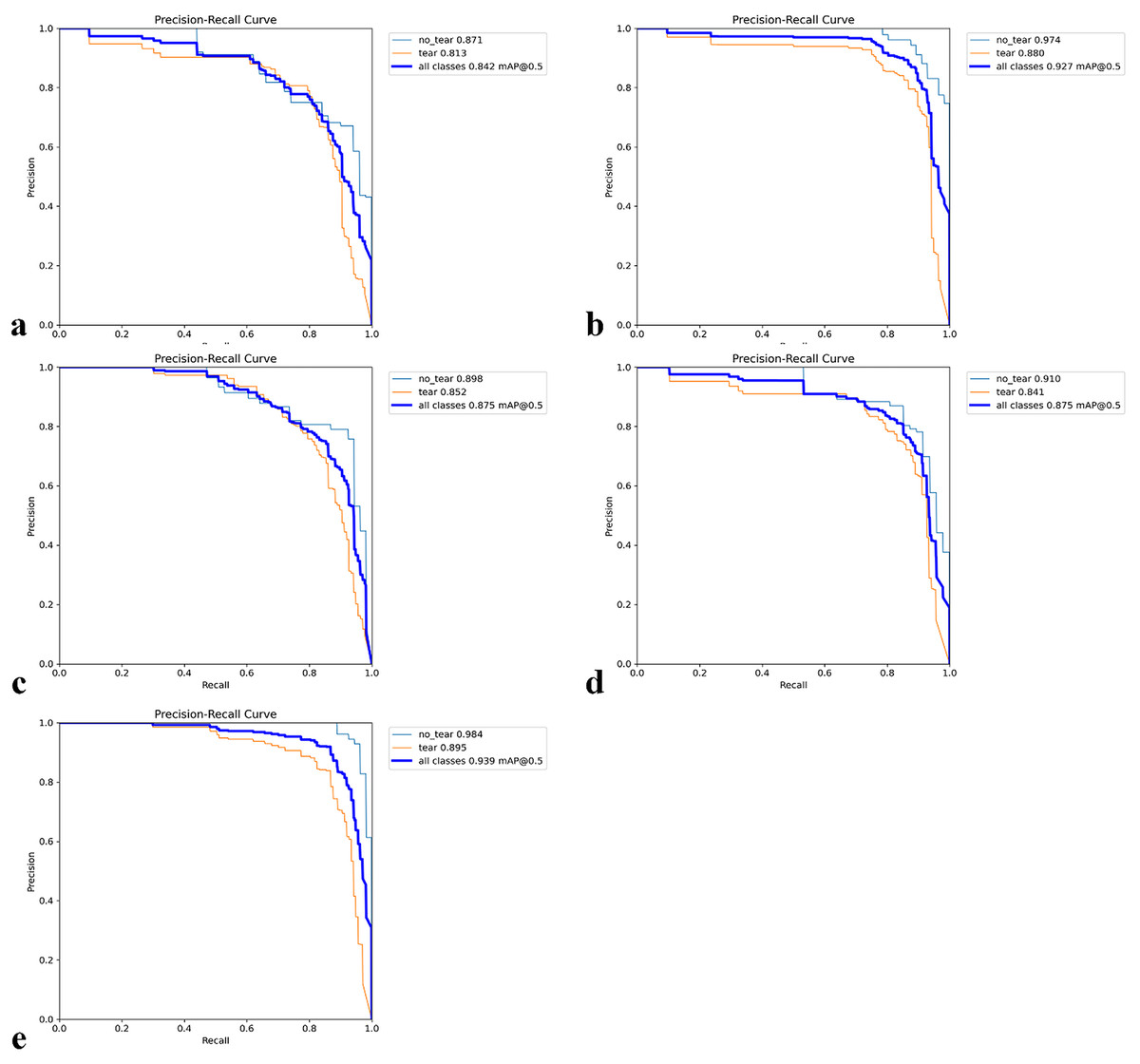
Figure 7: Precision–Recall (PR) curves for five-fold cross-validation.
(A–E) The PR curves for each fold together with the corresponding class-wise AP50 values.
A heatmap is used to gain insight into which areas of the proposed model are most discriminative in the image. Heatmaps are essential for the interpretation of DL models. HiResCAM was used to determine whether the model makes the correct decision by examining the relevant regions in the decision-making process. The heatmaps revealed that our model achieves high accuracy and that objects are particularly concentrated in the boundary regions (Fig. 8).
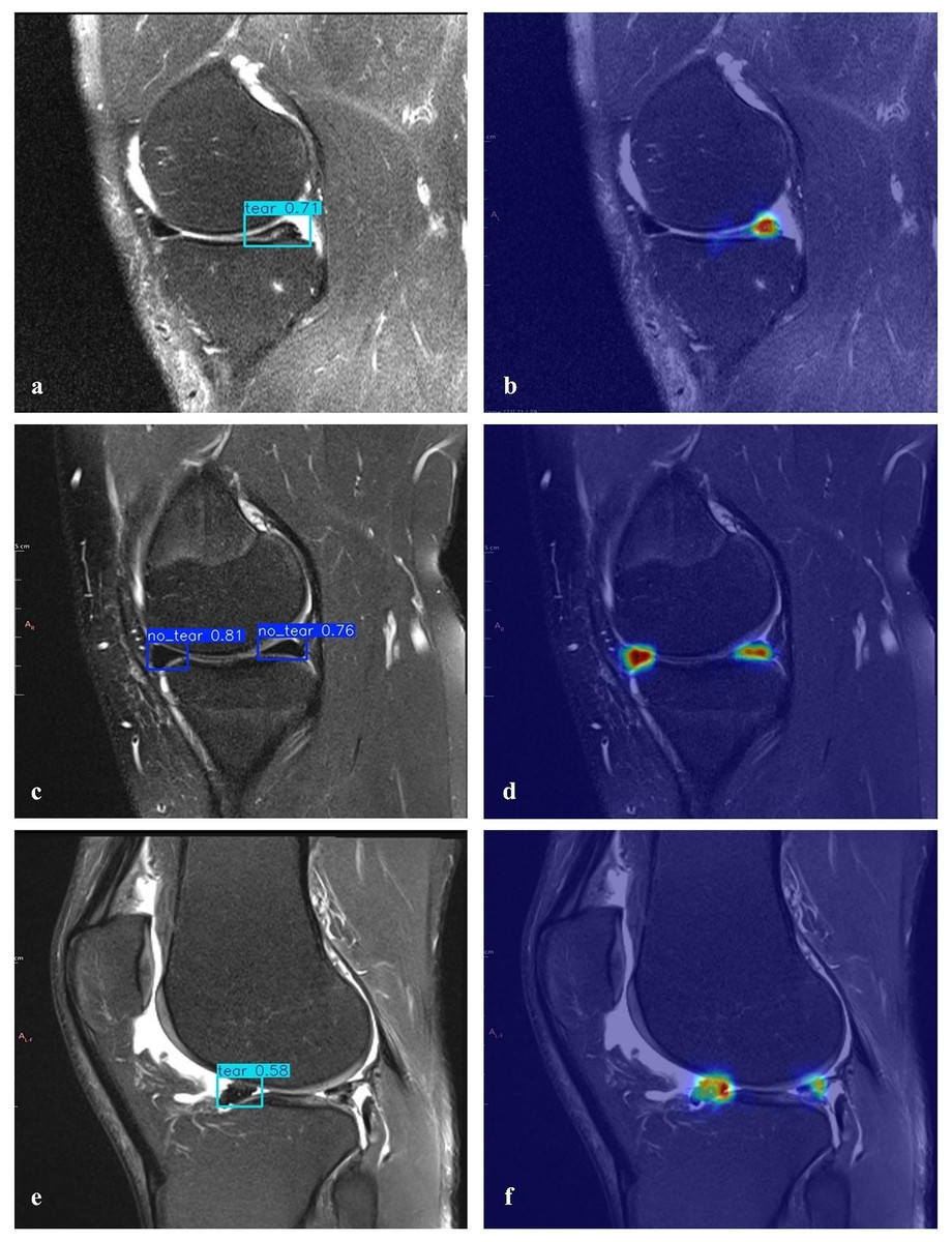
Figure 8: Detection of torn meniscus and corresponding heatmaps.
(A) Correct detection of a right knee medial posterior meniscal tear in the sagittal section and (B) the corresponding heatmap (true positive). (C) Correct detection of left knee medial anterior/posterior healthy menisci in the sagittal section and (D) the corresponding heatmap (true negative). (E) Incorrect detection showing a meniscal tear where none was present (false positive) and (F) missed detection of an existing meniscal tear (false negative).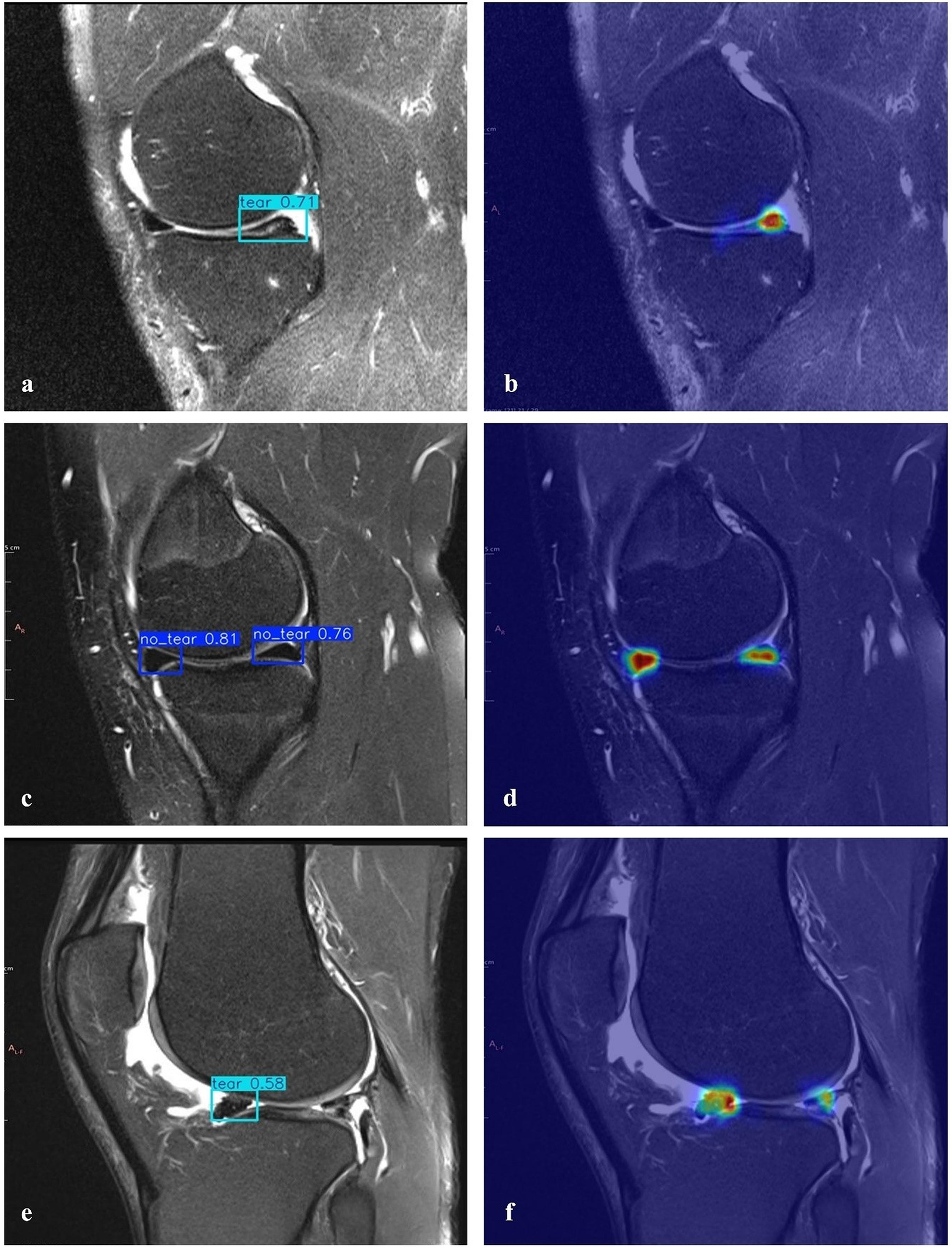
The proposed MOD-YOLOv8 architecture was compared not only with models of the YOLO family, but also with other SOTA architectures that are frequently used in the field of current object detection. For this purpose, the transformer-based models RT-DETR (Zhao et al., 2024a) and the multi-purpose detection system Detectron2 (Wu et al., 2019) were selected. In the literature, RT-DETR stands out for its high accuracy and generalization capacity, thanks to its advanced attention mechanisms, while Detectron2 is widely used due to its modular structure and success in various object detection tasks.
To ensure a fair evaluation during these comparisons, identical hyperparameter settings were favoured in the experimental setups, and no transfer learning was used. Additionally, the same data set and hardware environment were utilized. As shown in Table 5, the MOD-YOLOv8 model outperformed RT-DETR and Detectron2 in terms of precision, recall, mAP50, and F1-scores. These results show that MOD-YOLOv8 is superior not only to YOLO-based models, but also to powerful SOTA detection architectures with different structural approaches.
| Models | PLast | RLast | mAP50Last | F1-scoreLast |
|---|---|---|---|---|
| RT-DETR | 0.7275 | 0.6600 | 0.7043 | 0.6921 |
| Detectron2 | 0.8144 | 0.8700 | 0.8885 | 0.8413 |
| MOD-YOLOv8 | 0.8450 | 0.8902 | 0.9227 | 0.8671 |
Note:
P, precision; R, recall; mAP, mean average precision. Bold values indicate the best results obtained among all conditions or methods analysed for the respective metric.
Discussion
At the beginning of our experiments (October 2023–March 2024), YOLOv8 was the latest version widely used in stable and open medical imaging research. YOLOv10 (Wang et al., 2024) and YOLOv11 (Khanam & Hussain, 2024) were released after our pipeline was frozen, so we were unable to use them. Our primary goal is not only to migrate to the latest generic detector, but also to demonstrate that task-specific architectural improvements deliver reliable real-time performance on a clinically meaningful dataset. Therefore, the lightweight, optimized layers we have added to YOLOv8 are designed to be backbone-independent and can in principle be ported to future YOLO versions, and we plan to explore this porting in detail in the future.
In recent years, DL algorithms have improved, and data sets have increased. In this way, many AI-supported studies have been conducted in areas such as the detection of meniscal tears, characterization, orientation, and segmentation of these tears (Bien et al., 2018; Couteaux et al., 2019; Roblot et al., 2019; Saygılı & Albayrak, 2019; Saygili & Albayrak, 2020; Gaj et al., 2020). It shows that such applications can be used in clinical settings soon.
In YOLO-based studies conducted to detect meniscal tears, Şimşek & Sertbaş (2025) compared SOTA YOLO models using a dataset constructed from MRNet and reported that the YOLO9e model achieved the highest performance. In this study, the results were mAP50 = 0.9181, P = 0.8768, R = 0.9387, and F1-score = 0.9067. Similarly, Tlebaldinova et al. (2025) compared the effectiveness of the YOLO and RT-DETR family models for automatic detection and localisation of meniscal tears in MRI images and showed that YOLOv8x provided more stable and accurate results than RT-DETR. The YOLOv8x model achieved high scores in the main metrics: P 0.9580, R 0.9610, F1-score 0.9600, and mAP50 0.9750. The YOLOv4-based model developed by Hung et al. (2023) was trained and tested using 584 knee MRIs and achieved accuracies of 0.9540 and 0.9580 in the internal testing and validation datasets, respectively, and 0.7880 in the external validation dataset. In another study, Chou et al. (2023) showed that Scaled-YOLOv4 successfully localised the meniscus position (AUC: sagittal 0.9480, coronal 0.9630), while the EfficientNet-B7 model classified meniscal tears with high accuracy (AUC: sagittal 0.9840, coronal 0.9720). In addition, Güngör et al. (2025) evaluated the YOLOv8 and EfficientNetV2 models using a smaller dataset (642 knee MRIs). In this study, the YOLOv8 model achieved mAP50 values of 0.9800 in the sagittal view and 0.9850 in the coronal view, while the EfficientNetV2 model achieved AUC values of 0.9700 and 0.9800, respectively.
Previous studies have used CNN (Bien et al., 2018; Roblot et al., 2019) R-CNN, YOLO (Hung et al., 2023; Chou et al., 2023; Güngör et al., 2025; Şimşek & Sertbaş, 2025) EfficientNet, and transformer-based (Genç et al., 2025) models to detect meniscal tears. Some of these approaches have been used directly. In contrast, others have been integrated or applied as two-stage systems (e.g., one model to localise the meniscus region and another to classify tears). However, the number of studies that systematically include YOLOv8 in performance comparisons remains limited. The meniscus is a relatively small tissue, occupying less than 2% of the area in MRI images (Luo et al., 2024; Şimşek et al., 2025). In addition, the detection of meniscal tears is challenging due to the subtle differences between healthy and injured tissue, the small pixel area of the meniscus within the overall image, and the presence of detection differences, artefacts, and similarities between surrounding tissues. These factors negatively impact model performance and complicate MRI analysis. Therefore, specialised architectures are required for the reliable detection of such sensitive regions. In this context, the proposed MOD-YOLOv8 introduces lightweight, optimised, and interpretable modules that positively contribute to the accurate localisation and classification of meniscal tears, filling an essential gap in the literature.
Only data from the sagittal plane were used in this study. There are studies in the literature that focus exclusively on the sagittal plane (Vaishnavi Reddy et al., 2025; Zhou, Yang & Youssefi, 2025), the sagittal-coronal plane (Luo et al., 2024) and the sagittal-coronal-axial plane (Tanwar et al., 2025); however, the majority of research has focused on the sagittal plane. This is because the sagittal plane contains more information about the meniscus and provides a better characterisation of clinical patterns (Ma et al., 2023; Jiang et al., 2024). Nevertheless, the model also needs to be validated on coronal and axial images, as such validation would undoubtedly provide higher clinical validity. While previous studies have focused not only on the detection of meniscal tears (Güngör et al., 2025; Genç et al., 2025; Tanwar et al., 2025) but also on the characterisation of these tears (Rizk et al., 2021; Luo et al., 2024), the present study focused exclusively on the presence of the tear. This is one aspect of the study that needs further development.
For this study, a random sample from New York University’s FastMRI dataset was selected to create the working dataset. The dataset comprises individuals between the ages of 2 and 85, with an average age of 47.79, and is single-centered. FastMRI is not a dataset specifically developed for detecting meniscal tears, but instead consists of 10,012 DICOM images from 9,290 patients with various abnormalities. Access to images of healthy individuals is relatively limited, which has led to a class imbalance between cases with (681) and without (147) meniscal tears. This imbalance can lead to the model favouring more common conditions and recognising rare cases less accurately. To mitigate this problem, a five-fold cross-validation was performed, and the results showed that the model performed satisfactorily under these conditions. Although the age distribution of the dataset ranges from 2 to 85 years, the single-centre origin and the lack of diversity are factors that limit the generalisability of the model. In addition, the current dataset focuses solely on the presence of meniscal tears; characterisation of tear types or grades was not considered in this study. This is an area that requires further development. Future studies with larger, multi-center, and more diverse datasets will enhance the performance and clinical validity of the model. Additionally, utilizing synthetic minority oversampling technique (SMOTE) or other data augmentation techniques to balance the dataset in a controlled manner will further contribute to this goal.
A key limitation of this work is the use of a single-centre subset of the FastMRI dataset, comprising 471 patients and 828 sagittal images, which is relatively small compared to the diversity of knee MRI examinations encountered in routine clinical practice. The dataset was not originally curated for meniscal tear detection and shows a marked class imbalance (tear vs no tear), leading to potential selection and spectrum bias. Although these issues were addressed through stratified five-fold cross-validation, reporting of confidence intervals for all major metrics, and comparisons with several strong baselines under identical conditions, the generalisability of MOD-YOLOv8 to other institutions, MRI scanners, and imaging protocols remains uncertain. Nevertheless, it is important to note that several studies in the literature have used datasets of similar or even smaller scale for developing automated meniscal tear detection models. For example, Li et al. (2022) trained a 3D Mask-RCNN model using 546 knee MRI examinations, while Hung et al. (2023) used 584 MRI studies for automatic tear detection—both comparable in size to our dataset. These examples show that the dataset size used in the present study is consistent with prior work in the field. Future research should focus on validating—and, where necessary, adapting—the proposed architecture on larger, multi-centre cohorts and on datasets specifically designed for meniscal pathology, with improved representation of tear types and healthy controls.
It is in the like AI applications that decision-making processes are not easily interpretable. However, clinicians must trust the predictions of the models developed. To address this limitation and demonstrate the model’s interpretability, heat maps were utilized. As interpretability and reliability are essential for the clinical application of models, which require a high degree of confidence and validation, they need to be supported by additional structures. In the present study, the use of non-contrast MRI resulted in increased activation in the localisation of meniscal tears on the heat maps, which significantly contributed to and confirmed the diagnosis. On the other hand, one study in the literature described a patient who underwent radioiodine therapy for thyroid carcinoma and underwent whole-body FDG-PET for restaging due to a lesion detected on MRI of the knee. In addition, a tear was detected in the anterior horn of the right medial meniscus. Although whole-body FDG-PET showed no abnormal FDG uptake corresponding to the benign lesion in the right thigh, there was increased uptake at the level of the meniscal tear (El-Haddad et al., 2006). In that publication, meniscal tears were visualised by the FDG used in PET imaging, whereas in the present study, no external contrast agent was administered; instead, diagnosis was aided solely by algorithms developed from the source images. This shows that heat maps are a non-invasive method that can improve diagnostic accuracy.
Clinically essential points and perspectives of the present work include improving the accuracy of the MOD-YOLOv8 model in detecting meniscus tears in knee MRIs using deep learning techniques and the use of heat maps to aid radiologists in analyzing data and enhancing the interpretability of the MOD-YOLOv8 model’s predictions. Furthermore, to the best of our knowledge, this study is the first to introduce a MOD-YOLOv8-based algorithm for detecting meniscal tears in the literature.
In terms of clinical impact, the MOD-YOLOv8 model has the potential to reduce diagnostic time by enabling rapid automated assessments, which can be particularly useful in emergencies or when workloads are high. By minimising false negatives, the model can help to avoid misdiagnoses that could delay treatment, while false positives can be efficiently corrected by clinicians with minimal effort. Possible application scenarios include use as an assistant to the radiologist in routine practice, use as a second reader tool for less experienced clinicians, or use as a triage aid in mobile screening units.
The proposed model can detect meniscal tears but is not able to categorize them or identify other knee problems. Furthermore, it only provides results in the sagittal plane; evaluations in the coronal and axial planes could enhance the model’s performance. Creating a more balanced dataset and considering common medical conditions are crucial for achieving better results. Additionally, the model occasionally fails to identify a meniscal tear in specific images accurately. For example, in Fig. 8E, although there is signal enhancement indicating a tear in the posterior horn of the lateral meniscus of the right knee in the sagittal plane, contour irregularities and signal enhancement indicating degeneration in the anterior horn, as well as fluid in the knee joint, could be misinterpreted. However, in the heat map analysis (Fig. 8F), a low but prominent temperature value is detected in the correct region of the meniscal tear (posterior horn).
Table 4 shows a precision difference in favour of no_tear (0.9490 vs 0.8760, Δ ≈ 0.0730). This difference can be explained by the imbalance of the classes and the small target size, tear/no_tear boundary similarities, and the sensitivity of the conf/Non-Maximum Suppression (NMS) threshold. In addition, the high precision value of the no_tear class, which has fewer images, reflects that it is easier to detect because the region of interest (ROI) regions of the non-cracked meniscus do not contain anomalies. To achieve more stable results across classes, we recommend using class-weighted or focal losses, oversampling/balancing augmentation for minority classes, class-based confidence or NMS threshold scanning, hard-negative mining, and Test-Time Augmentation (TTA) applications. In addition, we plan to relabel examples with uncertainties in the labelling process by two experts in the future.
The receiver operating characteristic (ROC) analysis performed using image-level scores (maximum confidence per image for the tear class) for the MOD-Yolov8 model yielded an area under the curve (AUC) value of 0.9950 for the discrimination between tear and non-tear states, as shown in Fig. 9. This value is higher than those specified in the literature. This indicates that the model has excellent discriminative power. The ROC curve completes the PR-based evaluation by incorporating the rate of true negatives, providing a more comprehensive picture of the model’s diagnostic ability. These results demonstrate the robustness of the proposed MOD-YOLOv8 model in distinguishing tear and no_tear cases.
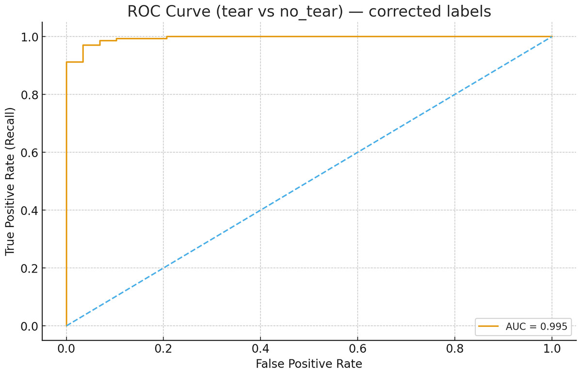
Figure 9: ROC curve for tear vs no_tear classification.
Figure 10 shows the curves of training and validation losses (box, cls, and dfl) over 100 epochs. Both the training and validation losses decrease steadily and reach a plateau, indicating that the model converges without signs of underfitting or severe overfitting.
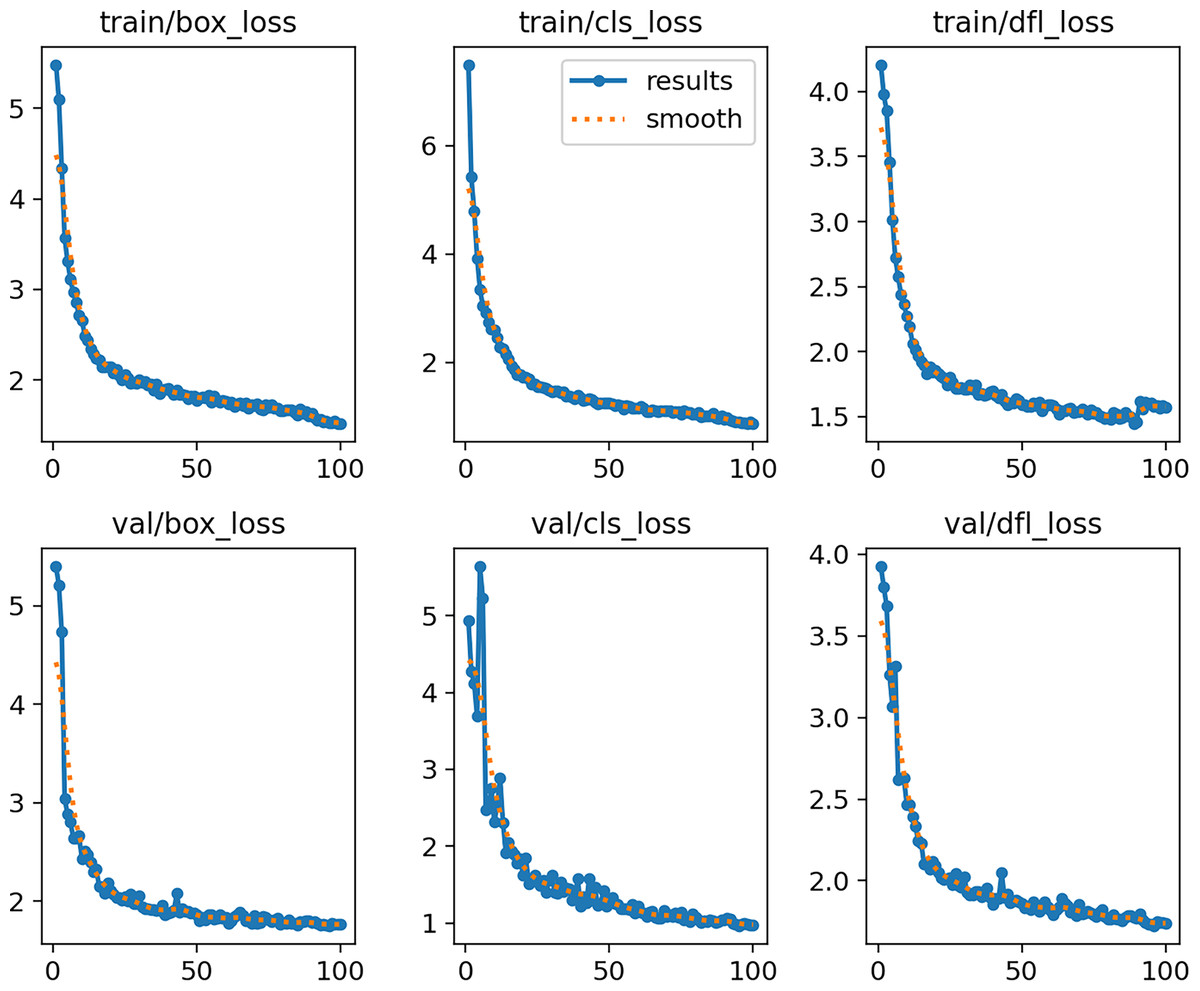
Figure 10: MOD-YOLOv8 training and validation loss curves across 100 epochs.
Conclusions
Although YOLO-based architectures for meniscal tears have been investigated in previous studies (Hung et al., 2023; Chou et al., 2023), no YOLOv8-based models are known. Some models detect meniscal tears in the sagittal plane only (Gaj et al., 2020; Ma et al., 2023), as well as those that consider both the sagittal and coronal planes (Bien et al., 2018; Tsai et al., 2020). In comparison, the MOD-YOLOv8 model shows superior performance in detecting meniscal tears. To further validate the effectiveness of the model and explore its applicability under various imaging conditions, it would be beneficial for future studies to utilize additional datasets.
This study presents MOD-YOLOv8, a deep learning model designed for detecting meniscal tears in sagittal knee MRI images. The model demonstrated superior performance compared to baseline YOLO architectures, providing reliable sensitivity and accuracy, and its interpretability was confirmed with heatmap visualizations. The findings suggest that MOD-YOLOv8 can reduce diagnostic errors and support less experienced clinicians, particularly in emergency settings or routine practice. A potential application scenario could be integrating the model into the daily workflow as a radiologist’s assistant or as a rapid screening tool in mobile emergency screening units. However, further improvements, such as validation with larger and more balanced datasets and inclusion of different meniscal tear types, are needed before it can be ready for clinical use. Future research may also explore the extension of the model to coronal and axial planes, validate it across multi-center datasets with diverse imaging protocols, and integrate it with automated hyperparameter optimization methods. Additionally, prospective clinical studies and real-time applications should be investigated to assess the model’s actual clinical utility. It should also be noted that the present study was limited to identifying the presence of meniscal tears without addressing their type, location, or severity. This limitation restricts the clinical applicability of the model as the characterisation of different tear patterns is of great importance for treatment planning. Therefore, the inclusion of tear characterisation in future work will be an essential step towards clinical translation.