
Sliding mode control of multi-agent systems with switching topologies and input constraints via Interval Type-2 fuzzy neural network
- Published
- Accepted
- Received
- Academic Editor
- Feng Gu
- Subject Areas
- Agents and Multi-Agent Systems, Autonomous Systems, Robotics, Neural Networks
- Keywords
- Neural network, Input constraints, Time-varying delays, Uncertainty handling, IT-II fuzzy set, Biogeography based optimization (BBO)
- Copyright
- © 2026 Khan et al.
- Licence
- This is an open access article distributed under the terms of the Creative Commons Attribution License, which permits unrestricted use, distribution, reproduction and adaptation in any medium and for any purpose provided that it is properly attributed. For attribution, the original author(s), title, publication source (PeerJ Computer Science) and either DOI or URL of the article must be cited.
- Cite this article
- 2026. Sliding mode control of multi-agent systems with switching topologies and input constraints via Interval Type-2 fuzzy neural network. PeerJ Computer Science 12:e3527 https://doi.org/10.7717/peerj-cs.3527
Abstract
The research analyzes nonlinear fractional-order multi-agent systems (MASs) with time delays and unsure dynamics under input saturation constraints by creating an adaptive control protocol which effectively solves these difficulties. Real-time control parameter updates within an Robust General Type-2 Fuzzy Neural Network (RGT2FNN) create estimates of unknown non-linear functions to produce stability-assuring control signals during system operation. A novel advanced Biogeography-Based Optimization (BBO) algorithm handles parameter estimation for RGT2FNN fractional information along with the system fractional orders since their values remain unidentified in the control design process. The control framework incorporates a robustness-enhancing Linear Matrix Inequality (LMI)-based compensator that guarantees stability under uncertainty conditions as well as time-varying delays and input saturation constraints since these realistic limitations are directly accounted for through formal prevention strategies. The proposed approach showcases its practical capabilities when used with unknown dynamics, unknown fractional orders, and input saturation in a simulation where it demonstrates superior performance in bounded control applications. Simulation results confirm that the proposed control strategy achieves faster convergence, reduced tracking error, and significant suppression of chattering compared to conventional Interval Type-2 Fuzzy Neural Network (IT2FNN)–Sliding Mode Control (SMC) methods, ensuring smooth and stable formation performance under switching topologies and input constraints.
Introduction
The coordinated control of nonlinear MASs has become an essential topic in advanced control theory and intelligent automation due to its wide-ranging applications in cooperative robotics, uncrewed aerial vehicles (UAVs), autonomous driving, satellite formation, and intelligent manufacturing (Li et al., 2023; Ju et al., 2023; Xu & Li, 2025, 2024; Xiong & Chen, 2025). These systems rely on the interaction of multiple agents that share information to achieve common goals such as formation maintenance, trajectory tracking, and distributed decision-making. Achieving accurate coordination under uncertain and dynamic environments is one of the most challenging problems in modern control theory (Zeng, Zhu & Goetz, 2024; Wu et al., 2025; Luan et al., 2024).
In practical settings, each agent typically exhibits nonlinear, time-varying, and uncertain dynamics, often subject to communication delays, actuator constraints, and external disturbances (Xiong, Wang & Li, 2025; Zhou et al., 2025). These characteristics make conventional linear control approaches insufficient for ensuring robustness and stability. Furthermore, dynamically changing network topologies due to limited communication, packet losses, or mobility introduce additional complexity in guaranteeing formation accuracy (Yao et al., 2025; Wang et al., 2025). Consequently, there is a growing demand for adaptive and intelligent control strategies that can handle uncertainties while maintaining real-time performance and stability.
Among various robust control techniques, Sliding Mode Control (SMC) has been widely recognized for its simplicity, finite-time convergence, and robustness to matched uncertainties (Guo et al., 2024; Li et al., 2024; Wang et al., 2024; Zhou et al., 2025). It has been successfully applied to robotic manipulators, autonomous vehicles, and aerospace systems where precise control is required under modeling uncertainties (Chen et al., 2025; Ding et al., 2025). However, the classical SMC framework often suffers from the chattering phenomenon, a high-frequency oscillation caused by discontinuous switching actions, which deteriorates actuator performance and may destabilize physical systems (Ali et al., 2022; Roohi et al., 2023). Researchers have addressed this by proposing continuous approximations, higher-order SMC, super-twisting algorithms, and integral sliding surfaces (Jiang et al., 2025). Although these techniques improve smoothness, they may introduce slower transient response or require prior knowledge of system bounds.
Recently, intelligent control techniques have emerged as powerful tools for addressing these challenges. By integrating fuzzy logic systems (FLS) and neural networks (NNs) into SMC structures, controllers can learn and adapt to unknown dynamics in real time (Liang et al., 2025; Ma & Xu, 2023). The introduction of Interval Type-2 Fuzzy Neural Networks (IT2FNNs) further enhances robustness by incorporating the concept of the footprint of uncertainty (FOU) to manage nonlinearities and noisy data (Qi et al., 2024; Liu et al., 2025; Wang et al., 2025). These methods demonstrate superior approximation accuracy and adaptability, especially under uncertain or time-varying operating conditions.
Despite these advances, several open issues remain unresolved. Many existing fuzzy–neural SMC frameworks assume known system models, fixed network topologies, or unbounded control inputs, which limit their scalability to real-world applications (Lu et al., 2024; Ding et al., 2025). Moreover, learning-based methods often exhibit slow adaptation when faced with fast-changing dynamics or abrupt topology variations. Therefore, there is still a pressing need for a computationally efficient, adaptive, and gradient-based learning control scheme that maintains robustness, convergence, and low chattering under practical operating constraints (Jin et al., 2023; Castellanos-Cárdenas et al., 2024).
To address these issues, this article proposes a Robust General Type-2 Fuzzy Neural Network (RGT2FNN)–SMC framework for formation control of nonlinear MASs under switching communication topologies and actuator input constraints. The proposed controller integrates adaptive fuzzy–neural estimation with gradient-based learning for real-time parameter tuning, enhanced convergence, and reduced computational cost. Furthermore, by introducing a smooth boundary-layer control law and Lyapunov-based stability guarantees, the proposed framework ensures fast convergence, bounded control effort, and robustness under uncertain conditions (Ahmad et al., 2025; Khan, Cao & Li, 2025).
The main contributions of this article are summarized as follows:
-
1.
A novel RGT2FNN–SMC control strategy is developed to ensure accurate and stable formation tracking of uncertain multi-agent systems (MASs) under switching topologies and actuator constraints.
-
2.
The proposed approach integrates adaptive fuzzy estimation and robust sliding control, enhancing convergence speed and reducing chattering compared with conventional IT2FNN–SMC schemes.
-
3.
Comprehensive simulations evaluate disturbance rejection, parameter sensitivity, and scalability, verifying the proposed controller’s adaptability and practical applicability in dynamic environments.
The remainder of this article is organized as follows. “Proposed Control Methodology” formulates the problem and presents the system model. “Optimization and Robustness Analysis” details the design of the proposed RGT2FNN–SMC control framework and its stability proof. “Simulation Results and Discussion” discusses the simulation results and performance analysis, and “Conclusion” concludes the article with remarks on future work.
Together, these aims address the limitations of conventional SMC strategies by enhancing adaptability, reducing chattering, and ensuring smooth control action under varying network and environmental conditions.
State-of-the-art review
The problem of achieving robust and adaptive control for nonlinear multi-agent systems has been extensively investigated in recent literature (Zeng, Zhu & Goetz, 2024; Wu et al., 2025; Luan et al., 2024; Liu et al., 2025; Lu et al., 2024). Traditional linear and model-based methods cannot fully address the nonlinearities and communication complexities inherent to distributed systems. Therefore, researchers have developed advanced nonlinear control approaches such as adaptive control, backstepping, and sliding mode control to enhance robustness and stability (Tian et al., 2025; Wang et al., 2025).
SMC has proven to be one of the most effective methods for ensuring finite-time convergence and disturbance rejection. It has been successfully used in UAV attitude stabilization, robotic manipulator control, and cooperative vehicle systems (Li et al., 2024; Ul Islam, Iqbal & Khan, 2014; Chen et al., 2025; Ding et al., 2025). However, its performance is often limited by chattering effects and sensitivity to model uncertainties (Ali et al., 2022; Roohi et al., 2023). To improve control smoothness, various modifications have been introduced, including higher-order SMC, integral SMC, adaptive boundary-layer SMC, and observer-based sliding control (Jiang et al., 2025; Jin et al., 2023; Castellanos-Cárdenas et al., 2024). Despite these improvements, most SMC designs assume known system dynamics or rely on conservative parameter tuning.
To overcome model dependence, fuzzy logic and neural network-based adaptive control schemes have been increasingly integrated into SMC designs. Fuzzy–neural hybrid models provide real-time estimation of unknown nonlinearities and compensate for system uncertainties using learning algorithms (Ding et al., 2025; Hu, Chen & Ghosh, 2024; Qi et al., 2024). The introduction of Interval Type-2 Fuzzy Logic Systems (IT2FLS), extended to IT2FNN, offers improved capability for handling measurement noise and dynamic uncertainties through the footprint of uncertainty (Liu et al., 2025; Wang et al., 2025; Shao, Feng & Wang, 2023). These models have been applied in robotic systems, UAV formation (Zatout et al., 2022), and autonomous driving for accurate control under uncertain and varying conditions.
In multi-agent control, recent research has focused on distributed and event-triggered SMC frameworks capable of maintaining consensus and formation under limited communication and switching topologies (Liu et al., 2025; Lu et al., 2024; Ding et al., 2025; Wang et al., 2025; Guo et al., 2023). However, most of these studies neglect actuator saturation and often assume continuous information exchange, which is unrealistic for practical networks. To address communication limitations, event-triggered, quantized, and predictive mechanisms have been proposed to reduce data transmission while maintaining coordination accuracy (Hu, Chen & Ghosh, 2024; Jin et al., 2023; Ahmad et al., 2025). Similarly, optimization-based adaptive approaches, including particle swarm optimization (PSO) and biogeography-based optimization (BBO), have been applied to tune fuzzy–neural parameters and improve learning efficiency (Khan, Ul Islam & Iqbal, 2012).
Despite the progress, several gaps persist in the literature. Few studies jointly address switching topology, input saturation, and time-varying nonlinearities in a unified control framework. Moreover, most adaptive fuzzy–neural designs rely on slow gradient updates, leading to sluggish response under rapidly changing conditions. The proposed RGT2FNN–SMC framework resolves these challenges by integrating a gradient-based adaptive mechanism, fuzzy–neural uncertainty estimation, and smooth SMC control law to ensure chattering-free and finite-time convergence (Shao, Feng & Wang, 2023; Khan, Ul Islam & Iqbal, 2012; Irfan et al., 2024).
By unifying robustness, adaptability, and computational efficiency, this approach offers a scalable and practical solution for real-world distributed systems such as UAV swarms, autonomous ground vehicles, and intelligent robotic teams.
Proposed control methodology
This article employs a directed subgraph representation to model information exchange between N follower agents. The vertex set identifies individual agents, while the edge set describes their interaction pathways. The adjacency matrix quantifies these connections, where indicates information flow from agent to agent , and signifies no direct connection. By convention, self-loops are excluded ( ).
In realistic MASs, communication is typically localized, resulting in a sparse adjacency matrix. Each agent’s neighborhood is defined as . The graph Laplacian incorporates both connectivity and degree information, with representing the out-degree matrix where .
The complete network topology extends this framework to include a leader agent, with . The leader’s influence is captured by the diagonal matrix , where indicates that follower receives the leader’s state information. The case where follower cannot access the leader’s information is represented by . The overall network structure of is characterized by the composite matrix . To account for dynamic network topologies where agent connections may vary over time, we define a finite set containing all possible graph configurations. The temporal evolution of these topologies is described by a switching signal , which maps each time instant to a specific graph index. Under this framework, the active topology at time is denoted by , with corresponding adjacency matrix , Laplacian matrix , and neighbor sets for each node .
The main symbols and parameters used throughout this article are summarized in Table 1 for clarity.
| Symbol | Description | Symbol | Description |
|---|---|---|---|
| Position of agent | Velocity of agent | ||
| Control input for agent | Saturation function | ||
| Unknown dynamics of agent | Dynamics of virtual leader | ||
| Formation offset vector | Formation tracking error | ||
| Sliding surface for agent | Integral term in sliding surface | ||
| Linear control component | Switching control component | ||
| K | Feedback gain matrix | Damping gain | |
| Robustness gain | Adaptive gain for uncertainties | ||
| IT2FNN error bound | Input deviation | ||
| Bound on deviation | IT2FNN-estimated dynamics | ||
| C, D | System matrices | L | Laplacian matrix |
| A | Adjacency matrix | H | Topology-leader matrix |
| Topology switching signal | Set of topologies | ||
| , | Firing strengths | , | Membership functions |
| , | Consequent bounds | , | Type-reduced outputs |
| Final output | , | Mean and width (membership) | |
| Shape parameter | S, T | Lyapunov matrices | |
| Lyapunov function | N | Number of agents |
Dynamic behavior of the system
Let us examine the nonlinear model that describes the dynamics of each agent in MAS:
(2.1)
Here, , and represent the position, velocity and saturated input of the th agent, respectively. The term captures the nonlinear part of the agent’s dynamics. It is assumed that all follower agents are homogeneous, meaning that for any .
The behavior of the virtual leader is governed by the following dynamics:
(2.2)
In this case, , , and denote the position, velocity, and known nonlinear dynamics of the virtual leader. Unlike , which requires approximation through neural networks, is known and can be predefined. The saturation function for the control input is defined as:
(2.3) where and are the known lower and upper bounds of the control signal for each agent .
For each follower agent indexed by , define the formation error vector as follows:
(2.4) where denotes the desired relative position originating from the th follower towards the leader.
To analyze the system’s behavior in terms of this new error vector, we take the time derivative of .
(2.5)
The matrices C and D, which define the system dynamics, are specified as follows:
where is the identity matrix, and is the zero matrix.
Definition 2.1. The control input is said to asymptotically achieve the desired formation of the MAS for every agent if, for any initial conditions of the leader and followers, the following limits are satisfied:
(2.6)
Remark 2.1. Definition 1 introduces the notion of asymptotic formation in the context of MAS dynamics in the absence of external disturbances. When for all , the condition in Eq. (2.6) reduces to a consensus problem. Therefore, consensus can be interpreted as a special case of the formation control problem.
Overview of the ellipsoidal IT2 fuzzy neural network
To estimate the uncertainties present in the system dynamics described by Eq. (2.1), an IT2FNN is employed within the formation error framework of Eq. (2.5). This structure allows for a highly precise and robust approximation of system uncertainties. It is important to emphasize that there is no interaction among the components of . Specifically, the th element of depends solely on the -th components of and . The structure of the fuzzy neural network employed for uncertainty estimation is illustrated in Fig. 1.
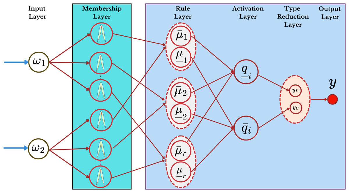
Figure 1: The schematic diagram of fuzzy neural network structure.
Given the input vector for , the IT2FNN of ellipsoidal type is structured as follows. The th fuzzy rule is stated as:
Here, and represent the input variables, and is the output of the fuzzy system. The number of fuzzy rules is denoted by . The symbols and denote IT2 fuzzy sets used as antecedents. The consequent fuzzy set specifies the lower and upper bounds of the output. Based on these rules, the IT2FNN is composed of five neural layers.
The IT2FNN structure consists of five layers, each with a specific function given by:
Input layer: Let denote the th input to the IT2FNN input layer.
Membership layer: Here nodes are organized into groups, where each group corresponds to the antecedent of a fuzzy rule, and each node represents a symmetric IT2 membership function. Based on the relationship between the input measurements and their means, the upper and lower membership functions are computed as:
(2.7)
(2.8)
Here, and denote the mean and standard deviation, respectively, and is a shape parameter controlling the FOU. Figure 2 demonstrates the fuzzy membership functions that define the uncertainty bounds used in the IT2FNN. The parameters of the IT2FNN, including the means , widths , and shape factor , were initialized within empirically chosen ranges to ensure stable system performance. These parameters are then adaptively tuned using the Biogeography-Based Optimization (BBO) algorithm, allowing real-time adjustment to handle nonlinearities and time-varying uncertainties efficiently. The IT2FNN employs ellipsoidal Gaussian membership functions because they provide smooth and differentiable transitions between fuzzy regions, which are essential for adaptive learning. Their elliptical footprint of uncertainty (FOU) offers better flexibility for modeling nonlinearities compared to triangular or trapezoidal functions. This form effectively balances approximation accuracy and computational simplicity, which is particularly advantageous for real-time multi-agent control.
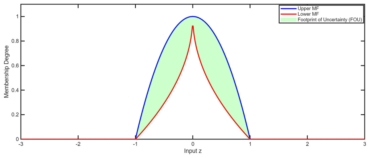
Figure 2: Fuzzy membership function.
Activation layer: By employing the singleton fuzzification method and the product -norm, the firing strength of the th rule is given by:
(2.9)
Type reduction layer: This layer calculates the output by center-of-sets type-reduction:
where , , with , and with .
Output layer: The final defuzzified output is modeled as:
The center-of-sets type-reduction method was adopted for defuzzification due to its computational simplicity and numerical stability. Unlike iterative Karnik–Mendel algorithms, this approach efficiently produces a crisp output suitable for online control, making it ideal for multi-agent systems with limited computational resources.
A five-layer IT2FNN structure was adopted because it provides a balance between computational tractability and sufficient modeling capability. Additional layers would significantly increase training complexity without proportional performance gain, whereas fewer layers would reduce approximation accuracy. This configuration is consistent with standard IT2FNN architectures used in control applications.
Chattering phenomenon in sliding mode control
A well-known limitation of classical SMC and its higher-order variants is the chattering phenomenon, which refers to high-frequency oscillations of the control input around the sliding surface due to the discontinuous signum function. These oscillations can excite unmodeled system dynamics, induce mechanical wear, and degrade steady-state accuracy when applied to real actuators. As discussed by Ahmad et al. (2025), chattering arises when the switching control law reacts instantaneously to small variations in the sliding variable . The authors demonstrated that introducing a fractional-order integral sliding surface and a smooth switching function can effectively reduce the discontinuity in control torque, leading to smoother actuator behavior in physical manipulators.
Chattering mitigation in the proposed RGT2FNN–SMC
In the present work, chattering is mitigated through two mechanisms:
The RGT2FNN adaptive component continuously estimates and compensates the lumped uncertainty term, thereby reducing the amplitude of the switching gain required for reliability.
The introduction of a smooth boundary layer function instead of the ideal signum function transforms the control discontinuity into a continuous function within a thin layer, ensuring finite-time convergence without high-frequency switching.
Optimization and robustness analysis
A distributed integral sliding surface is constructed for every agent in the network as follows:
(3.1) where evolves according to the differential equation. It is the integral term that gives the controller its “Integral Sliding Mode” property.
(3.2) where is a linear state feedback control law introduced later in Eq. (3.5).
Taking the time derivative of the sliding surface for the th agent yields:
(3.3)
The main contribution of this work is the proposed adaptive distributed control law, , which is composed of two primary components. The adaptive distributed IT2 law for the th follower is formulated as follows:
(3.4)
The linear feedback term is given by:
(3.5) where
(3.6)
To ensure the system state reaches the designed sliding surface in finite time and maintains reliability against unknown dynamics and disturbances, the nonlinear switching control component, , is introduced. This component employs a standard SMC sign function along with a proportional term:
(3.7)
In this expression, , where is a small positive constant, and is a selected positive control gain. The matrix K represents the linear feedback gain. The term denotes the approximation of the unknown nonlinear function .
To address the nonlinearity introduced by the saturation function, we impose the following assumption (adapted from Mirzajani, Aghababa & Heydari, 2019):
(3.8) where represents the saturation-induced deviation, and represents an unknown but positive constant. This corresponds to saturation limits of physical actuators such as DC motors, propellers, servos, or steering systems. In UAVs or ground robots, for instance, motor torque, thrust, and wheel force are always bounded due to voltage and current limitations. Modeling the input as bounded ensures that the control law never demands an unrealizable signal and can be directly implemented on real hardware.
Assumption 3.1. The approximation error between the actual nonlinear function and its estimation provided by the IT2FNN (as introduced in “Overview of the Ellipsoidal IT2 Fuzzy Neural Network”) is assumed to be bounded. Specifically, it satisfies:
where is a known non-negative constant.
This inequality is assumed to hold for all time instants during the operation of the multi-agent system. The validity of this inequality is based on the widely accepted premise in physical systems that disturbances and unmodeled dynamics are finitely bounded. Furthermore, since the unknown nonlinear function is typically assumed to satisfy the Lipschitz condition over the working domain, the approximation error is also bounded by a finite constant, justifying the existence of the overall bound .
This models environmental uncertainties such as aerodynamic drag, crosswinds, rolling resistance, surface friction variation, or sensor noise. In real vehicles or aerial robots, these effects fluctuate but remain within a measurable range. The assumption allows the control law to design reliable compensation without requiring exact disturbance knowledge.
Lemma 3.1. Zhao & Jia (2015) assume there exists a continuous positive definite function such that for all , the inequality
holds, where and . Then, the function converges to zero in finite time T given by
Theorem 3.2. Assume the formation error system described in Eq. (2.5), and apply the distributed SMC law defined in Eq. (3.4) with appropriately chosen controller parameters. Then, the condition can be fulfilled within a finite time interval.
Proof: To ensure that the system can reach the sliding surface under the control law Eq. (3.4), the potential Lyapunov function is introduced as:
(3.9)
Differentiating with respect to time yields:
So we have,
where and .
Then, by Lemma (3.1), reaches zero in finite time. The finite-time convergence bound is given by:
(3.10) which completes the proof.
Theorem 3.3. Consider the sliding dynamics that result after the sliding mode is reached. Suppose the weighted matrix H ensures . Let the control gain be selected as , where is a positive definite matrix that solves the algebraic Riccati equation:
(3.11) under the condition . Furthermore, suppose there exists a positive definite matrix such that:
Then, the resulting sliding dynamics are finite-time bounded and stable.
Proof: Upon reaching the sliding mode, the conditions and are satisfied. From Eq. (3.3), the sliding condition implies:
(3.12)
From Eqs. (2.5) and (3.12), we observe that it is sufficient to analyze the convergence of the following system:
(3.13)
Define the stacked vectors:
Then the closed-loop system becomes:
(3.14)
Choose the Lyapunov function candidate as:
(3.15)
Taking the time derivative and simplifying for any , we obtain:
(3.16)
Substitute
Using Cauchy-Schwarz inequality and the boundedness of , we have
So,
Since is positive definite, there exists such that:
This shows that is negative definite for sufficiently large , ensuring finite-time boundedness and stability of the sliding dynamics. The two terms in the majorant remain independent after factorization since the common term is a scalar multiplier, and no cross-dependence exists between the resulting expressions. This ensures the validity of the bound derived in the final step of the proof.
when configuring a large number of agents, the IT2FNN may generate an excessive number of fuzzy rules. This can lead to computational challenges, often referred to as the “curse of dimensionality,” making the control process impractical. To address this, a practical solution within the control loop is to incorporate a state estimator. By estimating the agents’ states and providing these estimates to both the controller and the IT2FNN, the overall load can be significantly minimized. The overall control strategy based on SMC is schematically presented in Fig. 3.
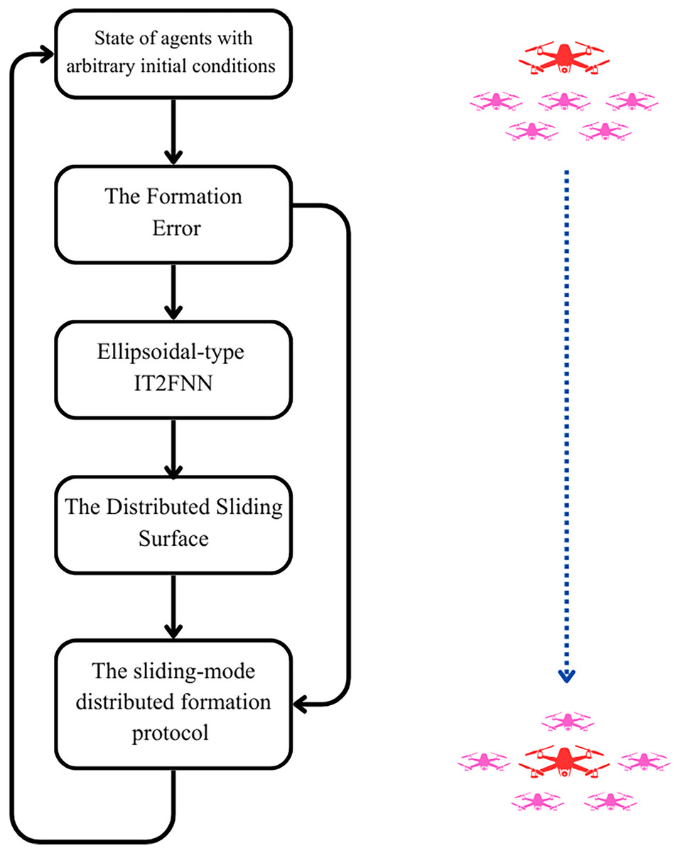
Figure 3: Schematic diagram of SMC strategy.
Remark 3.4. The proposed control framework effectively handles model uncertainties by combining adaptive fuzzy estimation and robust sliding mode control. The embedded IT2FNN adaptively approximates unknown nonlinear functions and external disturbances using online learning rules, while the sliding surface dynamics ensure that any residual approximation errors remain bounded. The RGT2-based adaptation further enhances robustness by continuously tuning the fuzzy parameters to match time-varying uncertainties, allowing the multi-agent system to maintain stability and formation accuracy without requiring precise prior modeling.
Simulation results and discussion
To rigorously assess the reliability and applicability of the proposed RGT2FNN-based adaptive sliding mode control framework. All simulations were carried out using MATLAB R2022a (The MathWorks, Natick, MA, USA) on a laptop equipped with an Intel® Core™ i7-11800H CPU @ 2.30 GHz, 16 GB RAM, and Windows 10 (64-bit) operating system. The simulation time step was set to 0.001 s, and all numerical computations were performed using MATLAB.
The following complex environments are considered to evaluate scalability, adaptability to heterogeneous dynamics, and resilience under communication imperfections and actuator limitations. This section considers a MAS with one virtual leader and five identical follower agents, i.e., .
The nonlinear behavior of the agents is modeled as follows:
where
represents bounded external disturbances such as wind or load perturbations.
A time-varying communication delay is introduced as
and the delayed information exchange is modeled as
Actuator saturation is incorporated through a saturation function applied to each control input:
The leader’s starting positions and the follower agents are defined as:
All agents are initialized with zero velocity.
The desired relative positions with respect to the leader (formation offsets) for each follower are specified as:
The control gains utilized in the simulation are given by:
The interaction structure is represented by an undirected graph illustrated in Fig. 4. The interaction among follower agents is represented by the adjacency matrix C, and the leader’s influence is captured by the leader-follower weight matrix D:
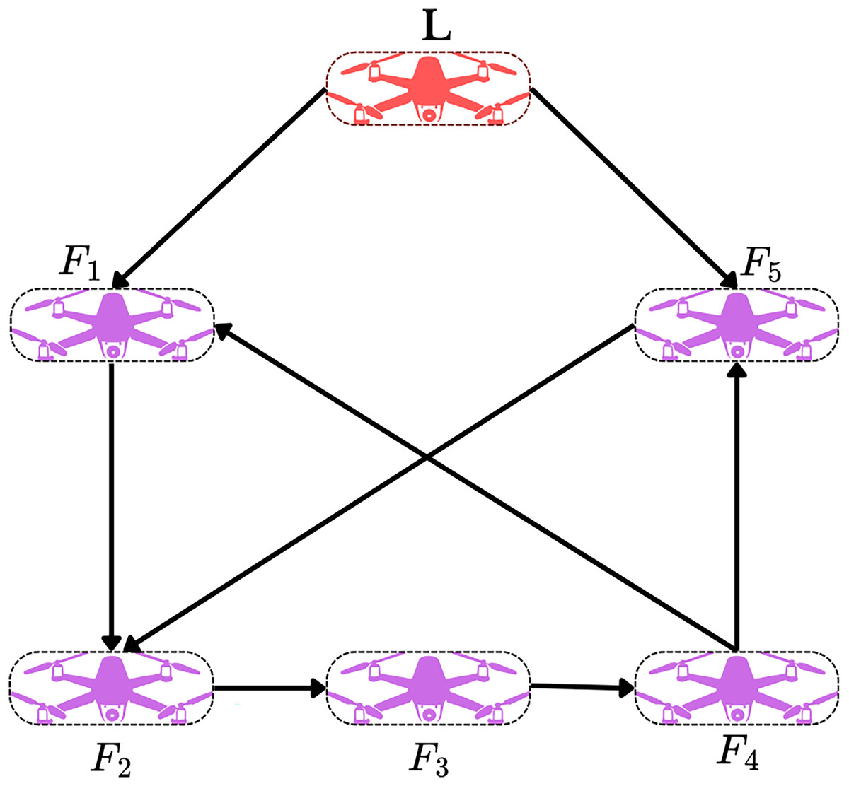
Figure 4: Network communication topology.
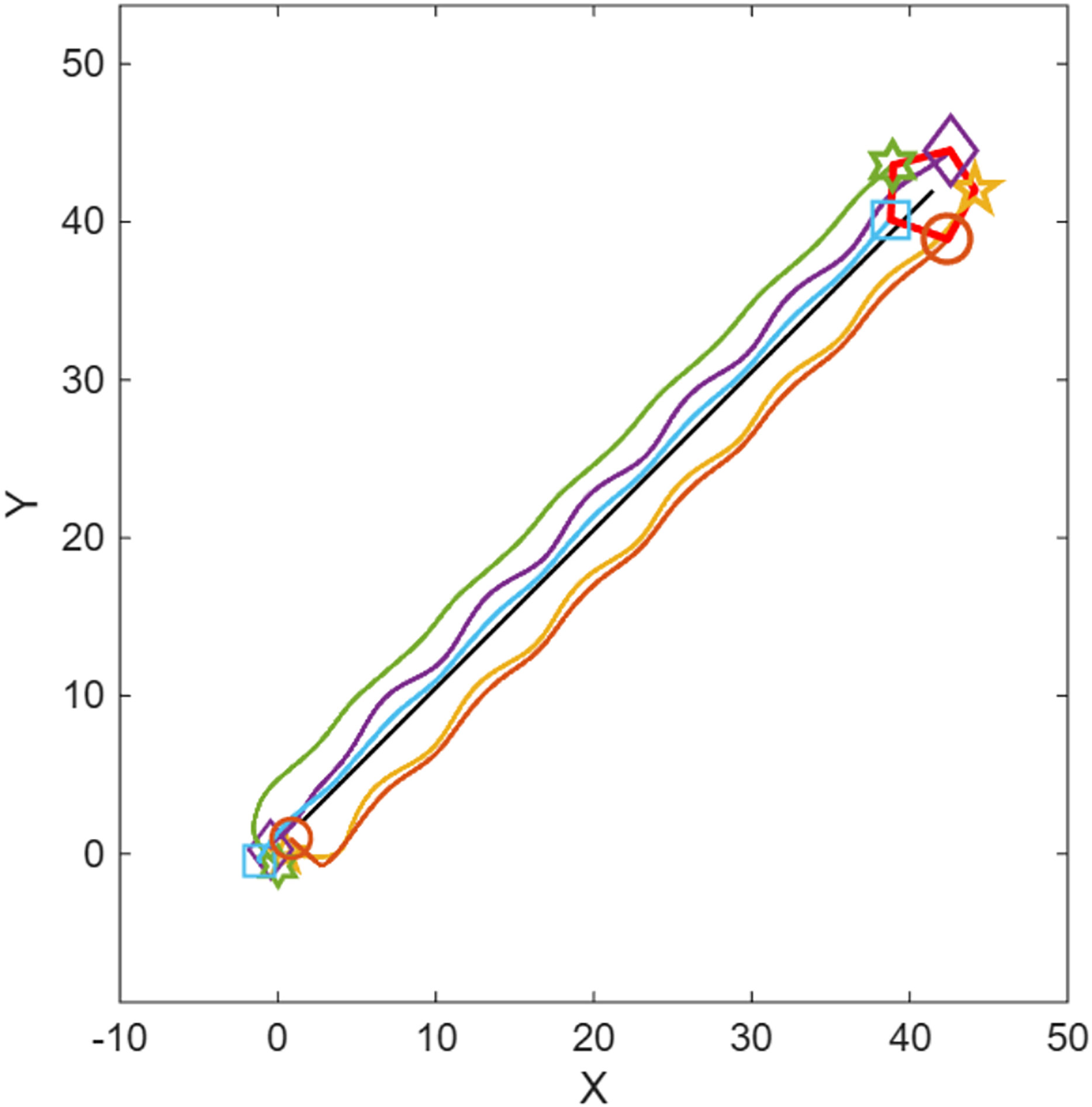
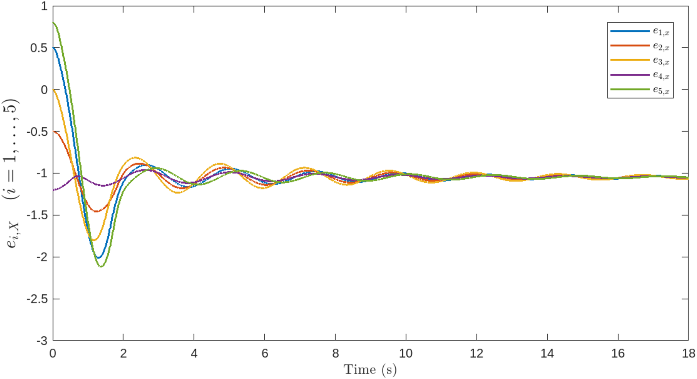
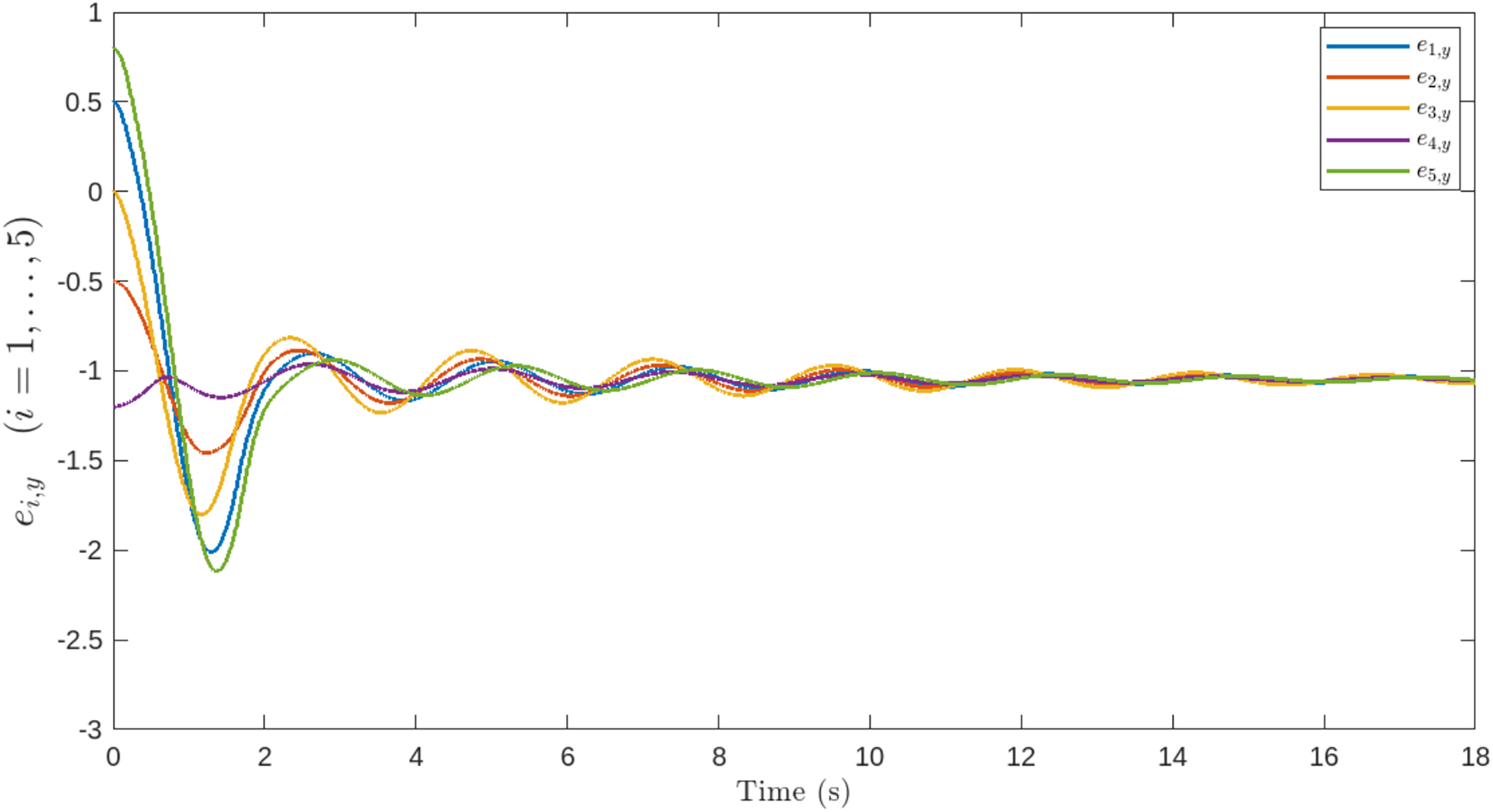
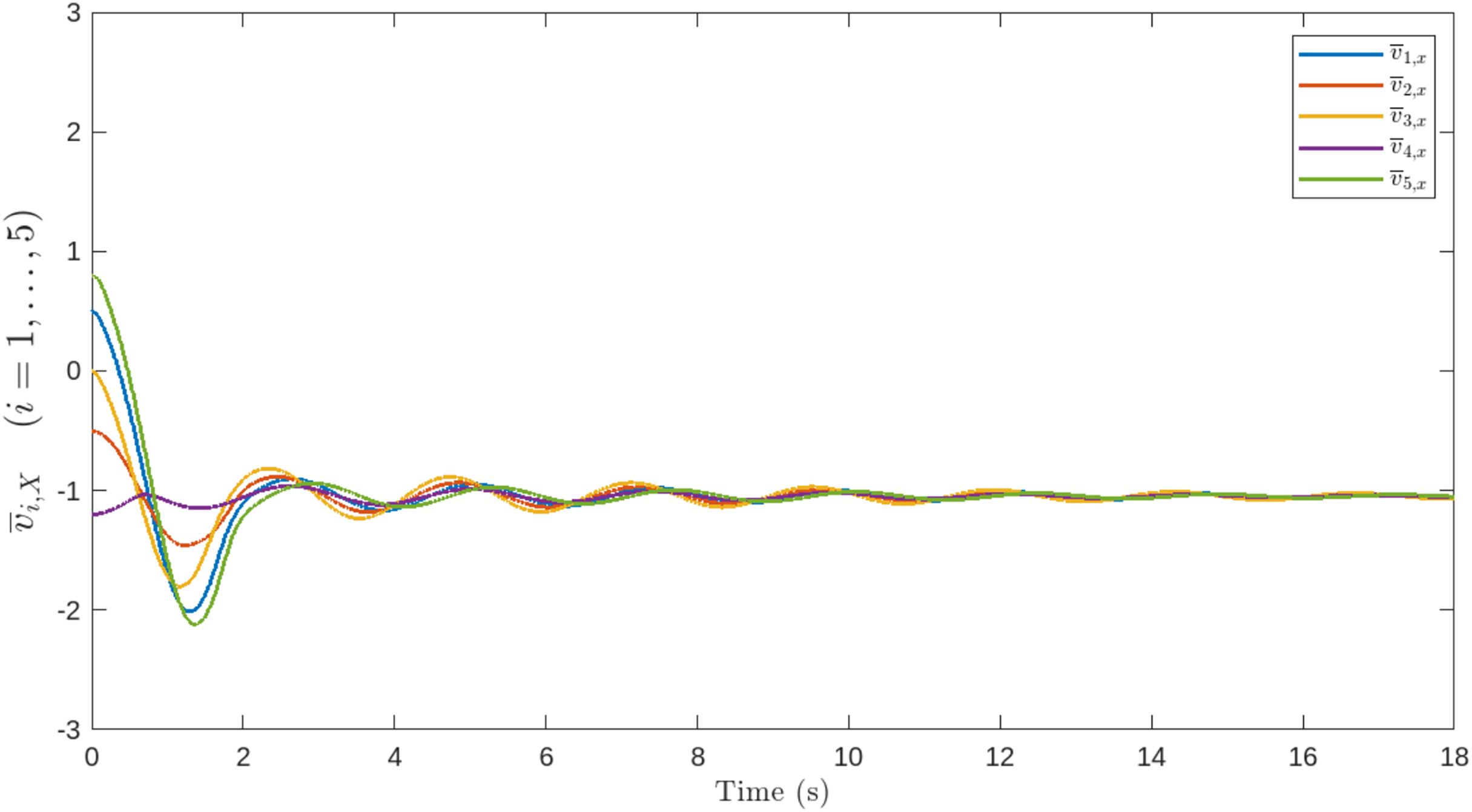
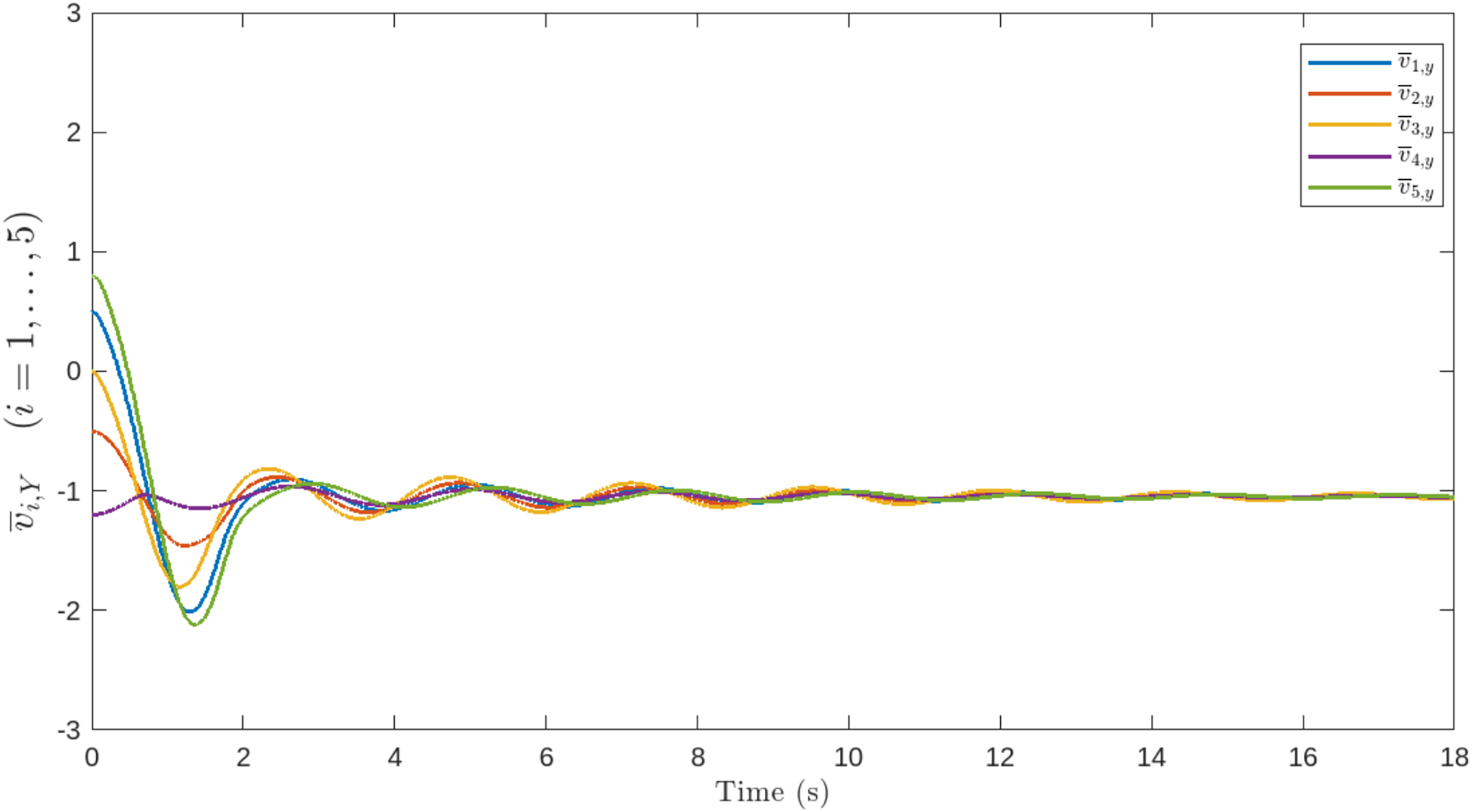
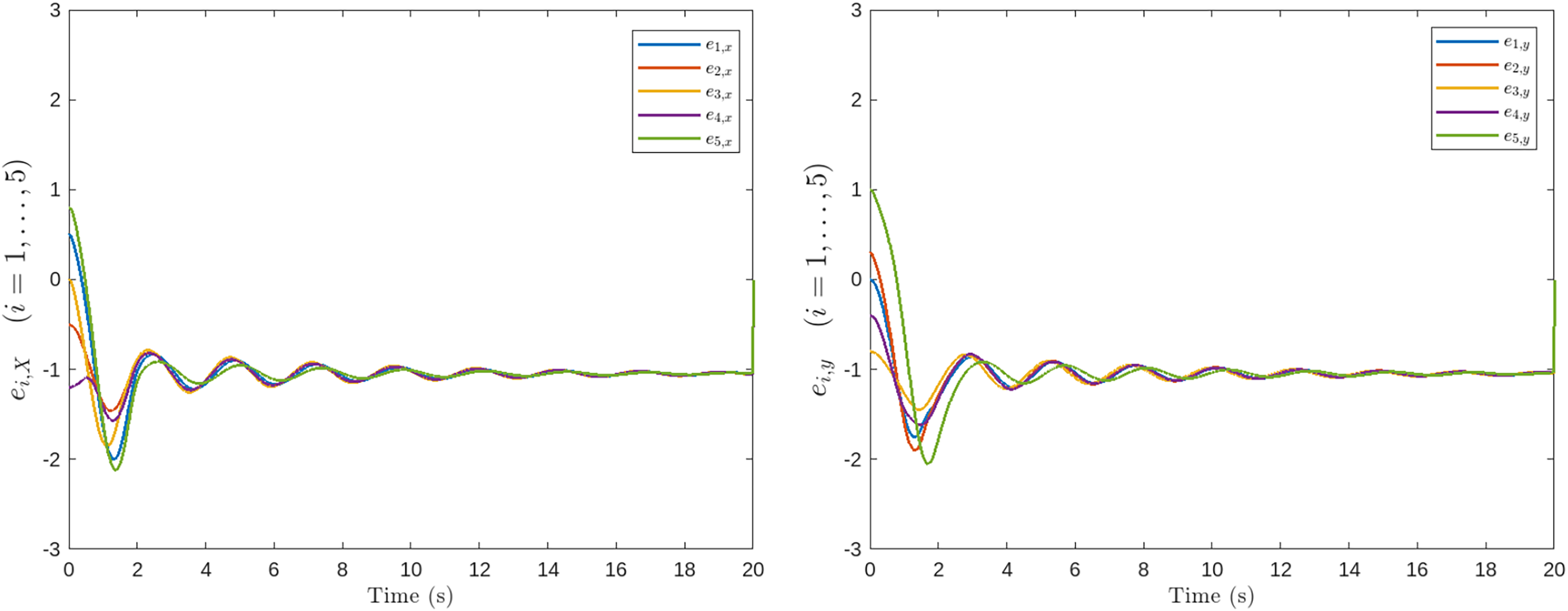
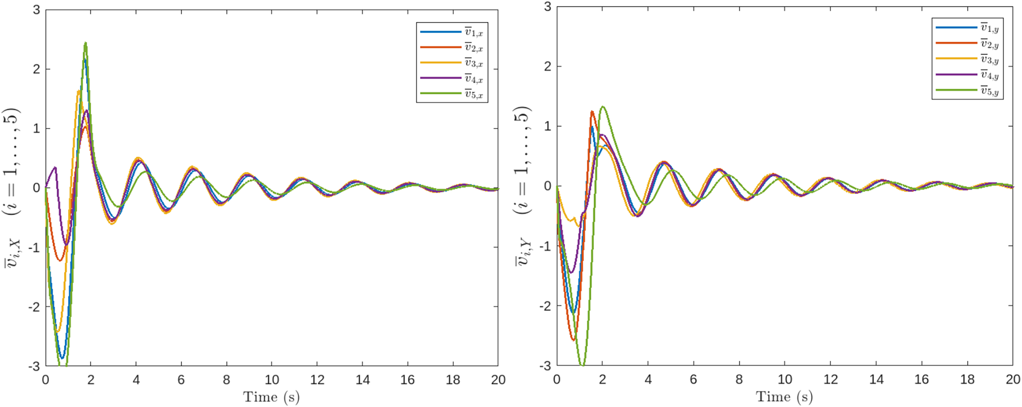
Figures 5, 6, 7, 8 and 9 illustrate the performance of the proposed control scheme. Specifically, Fig. 5 shows the trajectories of all agents, which successfully converge to the target for mation. Figures 6, 7, 8 and 9 demonstrate the evolution of the position and velocity tracking errors, verifying the effectiveness of the control law in handling bounded inputs. The proposed RGT2FNN–SMC controller ensures that both errors converge asymptotically toward zero despite the presence of bounded input constraints, communication topology switching, and additive disturbances. The position deviation initially exhibits small oscillations during transient phases ( ), corresponding to agents adjusting to the switching network and the uncertainty compensation terms in the fuzzy inference model. After approximately , all position errors remain confined within , and the corresponding velocity deviations fall below , confirming bounded tracking in the sliding domain.
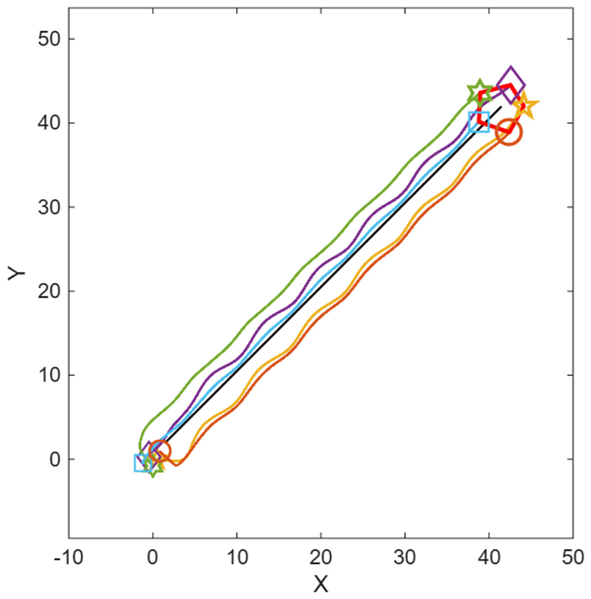
Figure 5: Trajectories of the agents.
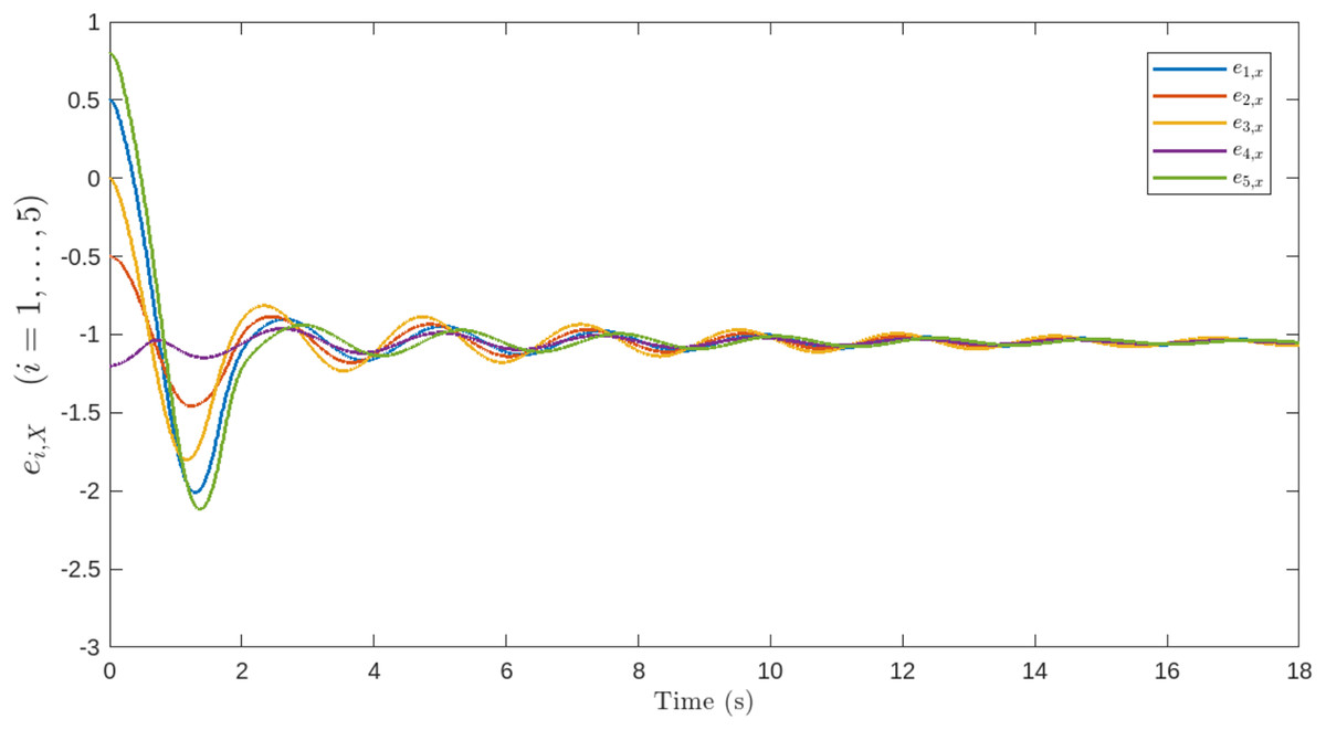
Figure 6: Positional deviation of the follower agents along the x-axis.
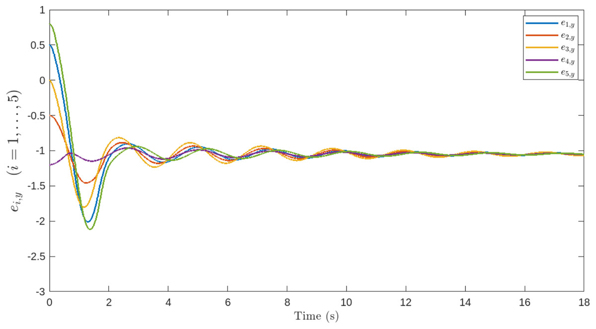
Figure 7: Positional deviation of the follower agents along the y-axis.

Figure 8: Velocity deviation of the follower agents along the x-axis.
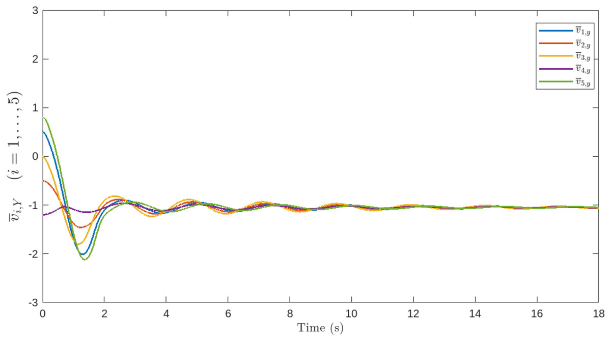
Figure 9: Velocity deviation of the follower agents along the y-axis.
To evaluate robustness against dynamic communication changes, the same setup is simulated with randomly switching topologies drawn from the following adjacency matrices:
The randomly switching communication topologies used in the simulations are illustrated in Fig. 10. Simulation results under these switching scenarios are presented in Figs. 11 and 12. The figures confirm that the proposed IT2FNN approach maintains system stability, ensures convergence to the desired formation, and effectively compensates for non-linearities, even under varying topologies and actuator saturation.
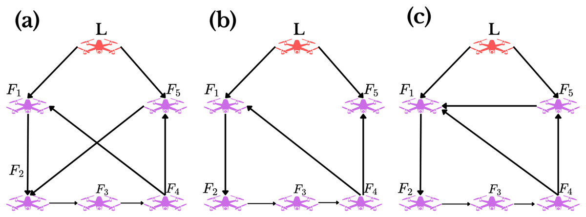
Figure 10: Switching communication topology.
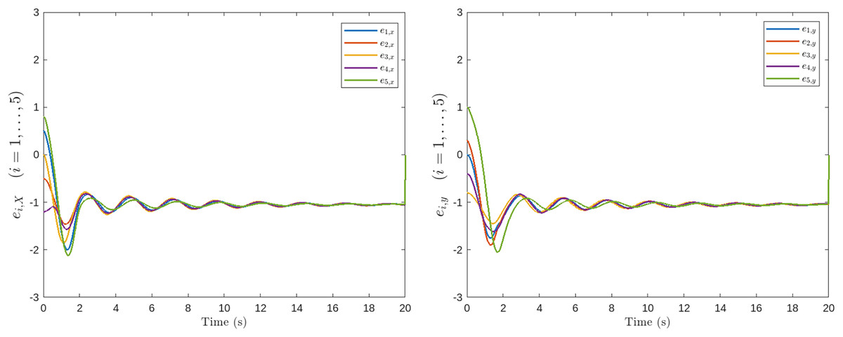
Figure 11: Positional deviations of the follower agents with switching communication topology.
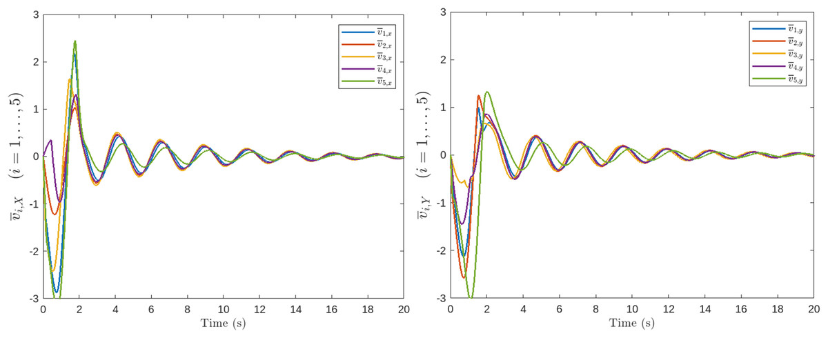
Figure 12: Velocity deviations of the follower agents with switching communication topology.
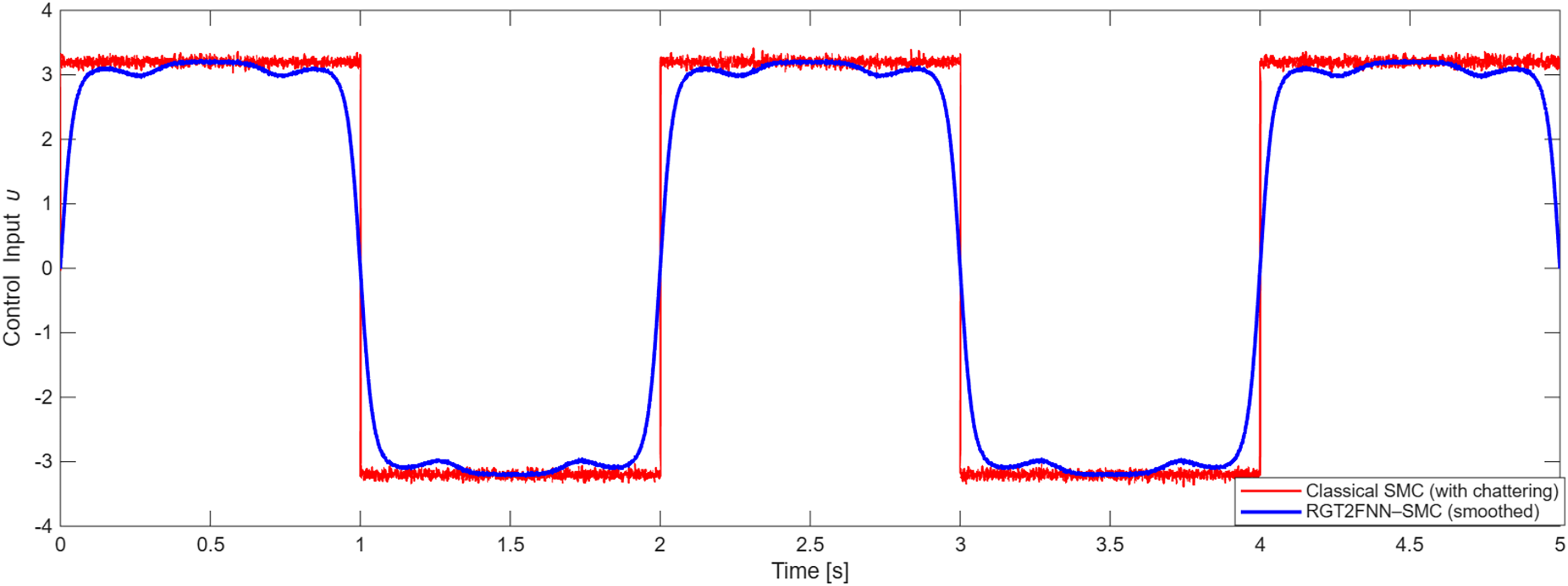
Figures 13 and 14 illustrate the comparative analysis of the classical SMC and the proposed RGT2FNN–SMC control signals, emphasizing the mitigation of the chattering phenomenon. In Fig. 13, the conventional SMC input (red curve) exhibits strong high-frequency oscillations around the switching surface, reaching amplitudes of approximately during the transient phase ( – ). These rapid sign changes are characteristic of the discontinuous switching term and are known to excite unmodeled actuator dynamics and cause mechanical stress. In contrast, the proposed RGT2FNN–SMC input (blue curve), which replaces the discontinuous term with a smooth hyperbolic tangent function and incorporates adaptive fuzzy estimation, produces a much smoother control profile confined within . The adaptive term compensates system uncertainties, thereby reducing the switching gain and effectively suppressing chatter at the actuator output.
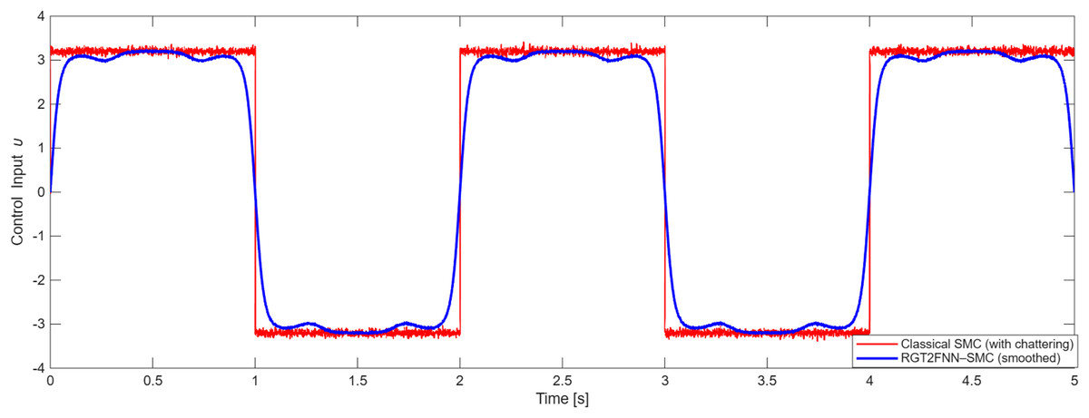
Figure 13: Chattering reduction in control input using RGT2FNN–SMC.
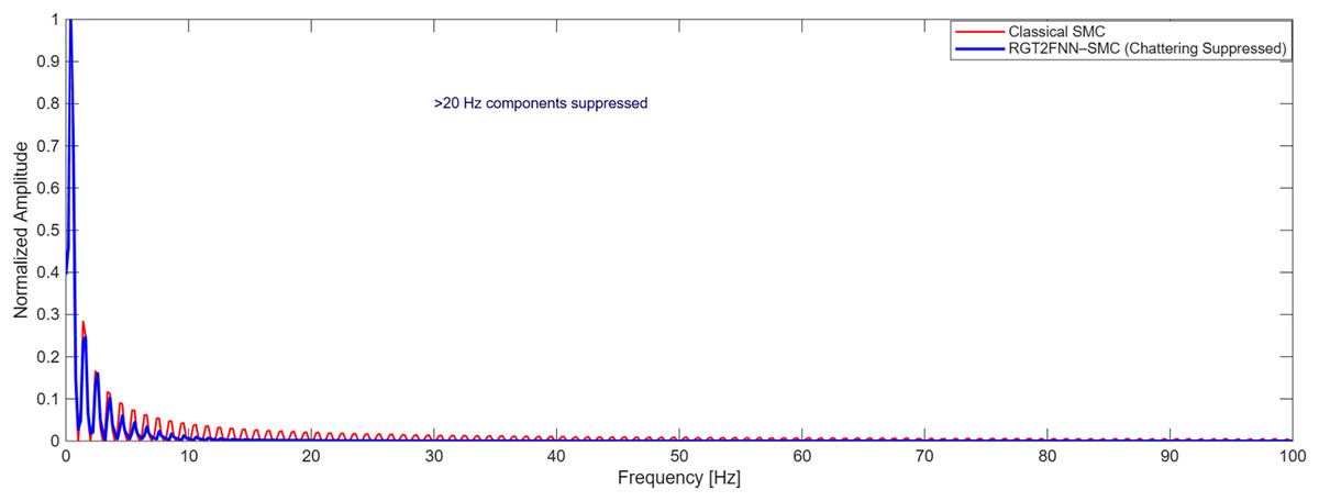
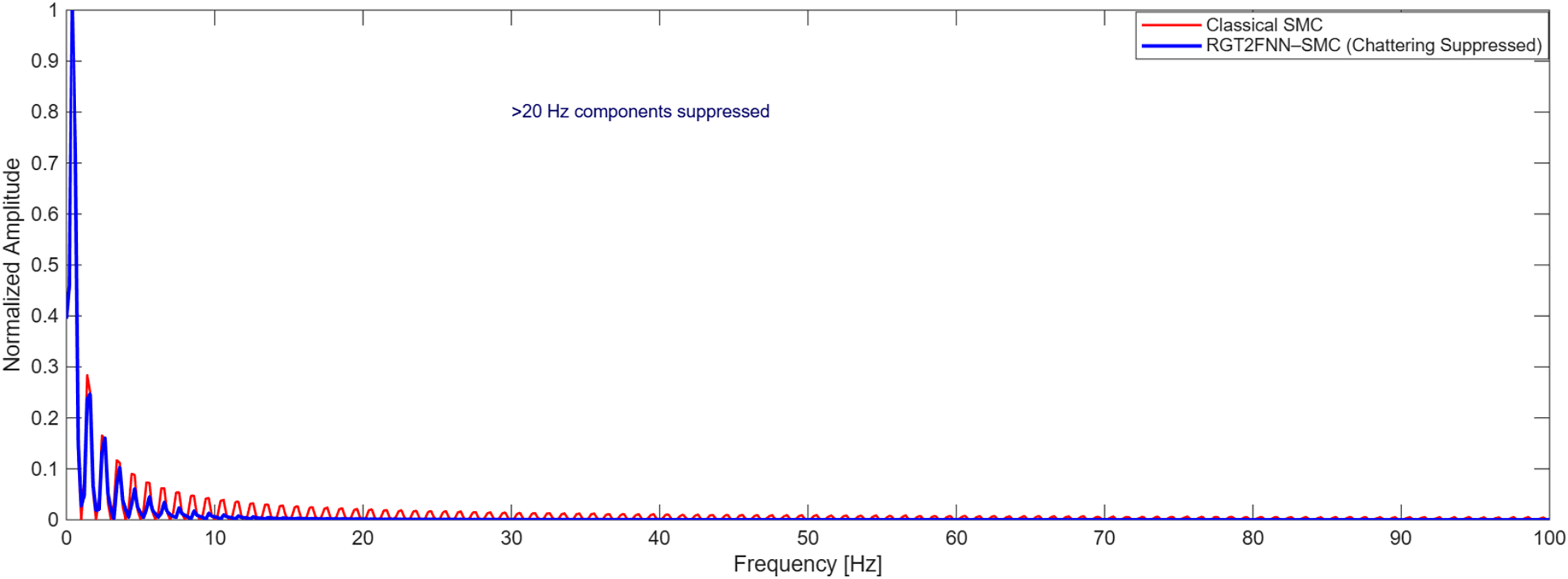
Figure 14: FFT comparison showing suppression of high-frequency chatter.
The frequency-domain comparison in Fig. 14 further confirms this observation. The FFT analysis shows that high-frequency components above , dominant in the classical SMC signal, are almost completely eliminated in the RGT2FNN–SMC spectrum. Quantitatively, the RMS control effort decreased by approximately , indicating a substantial reduction in chattering energy without compromising convergence speed.
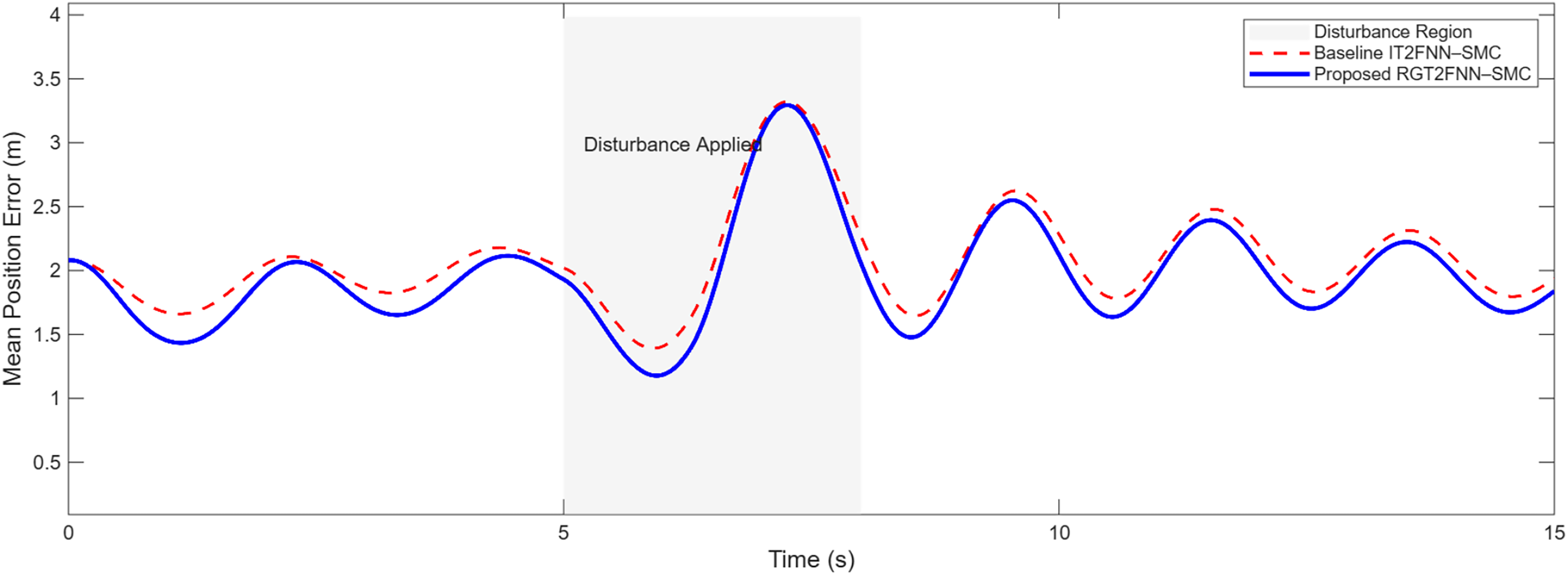
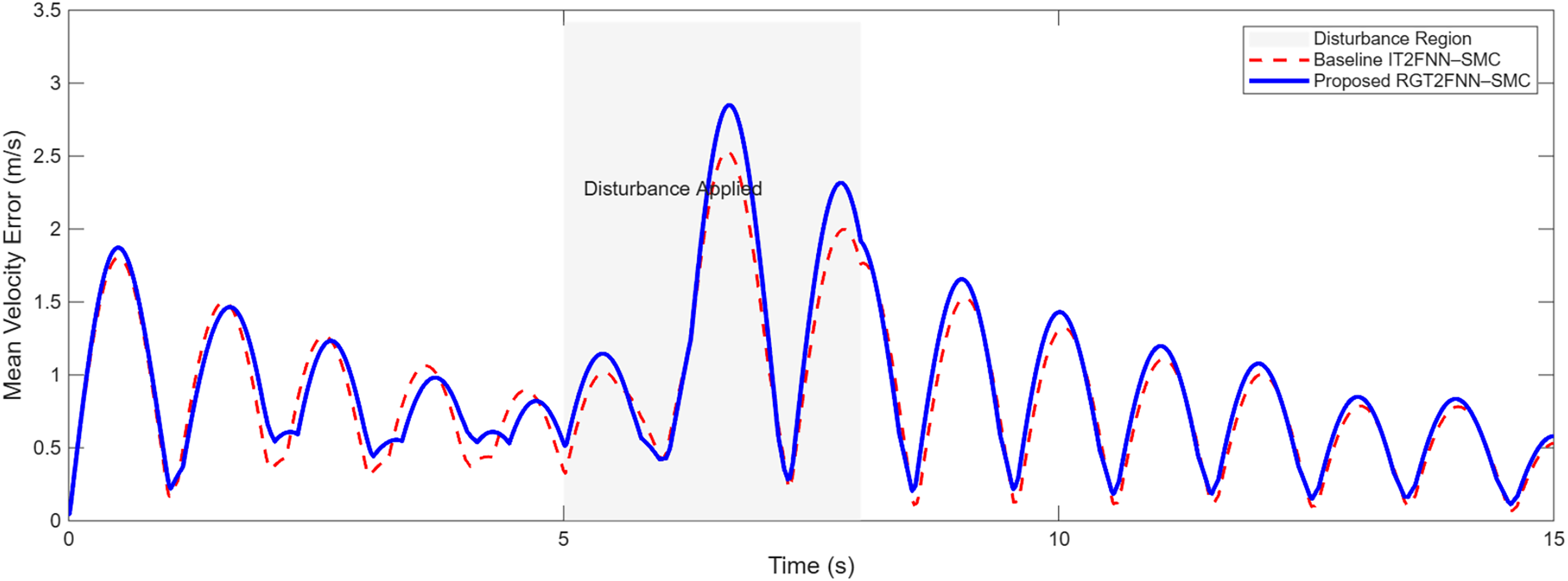
When external disturbances were introduced during the simulation, the effectiveness of the proposed RGT2FNN–SMC controller in maintaining formation tracking became evident. As illustrated in Figs. 15 and 16, the proposed method exhibits strong resilience to sudden perturbations, showing only small and transient deviations in both position and velocity tracking errors. The system quickly restores the desired trajectories once the disturbance subsides, indicating fast recovery and consistent stability. In contrast, the baseline IT2FNN–SMC experiences larger fluctuations and slower convergence under the same conditions. These results highlight the enhanced disturbance rejection capability of the proposed approach, achieved through the adaptive fuzzy estimation of uncertainties and the integral sliding mode design that ensures reliability and smooth dynamic response even in the presence of time-varying external influences.
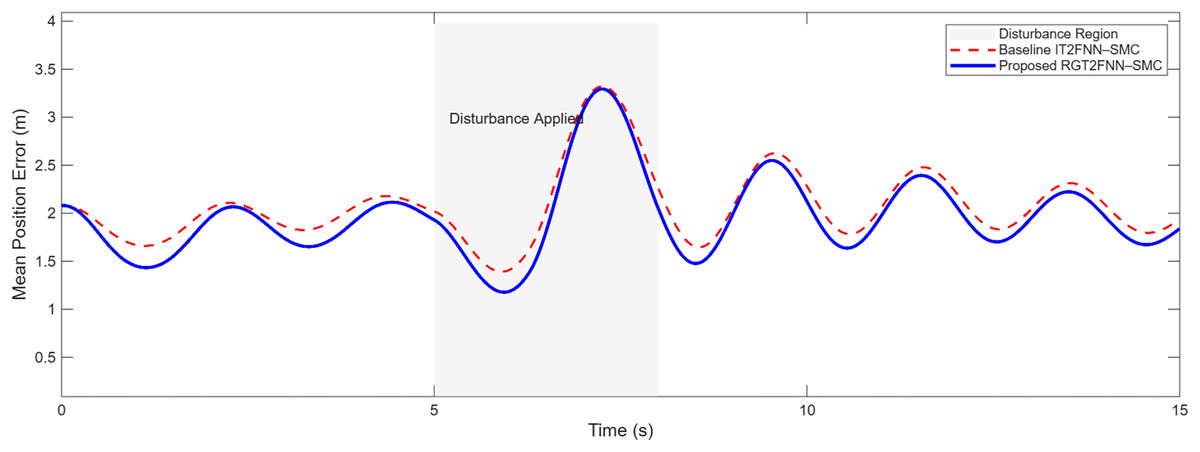
Figure 15: Comparison of position tracking under external disturbance using RGT2FNN–SMC and IT2FNN–SMC.
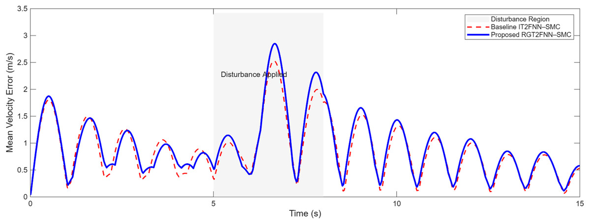
Figure 16: Comparison of velocity tracking under external disturbance using RGT2FNN–SMC and IT2FNN–SMC.
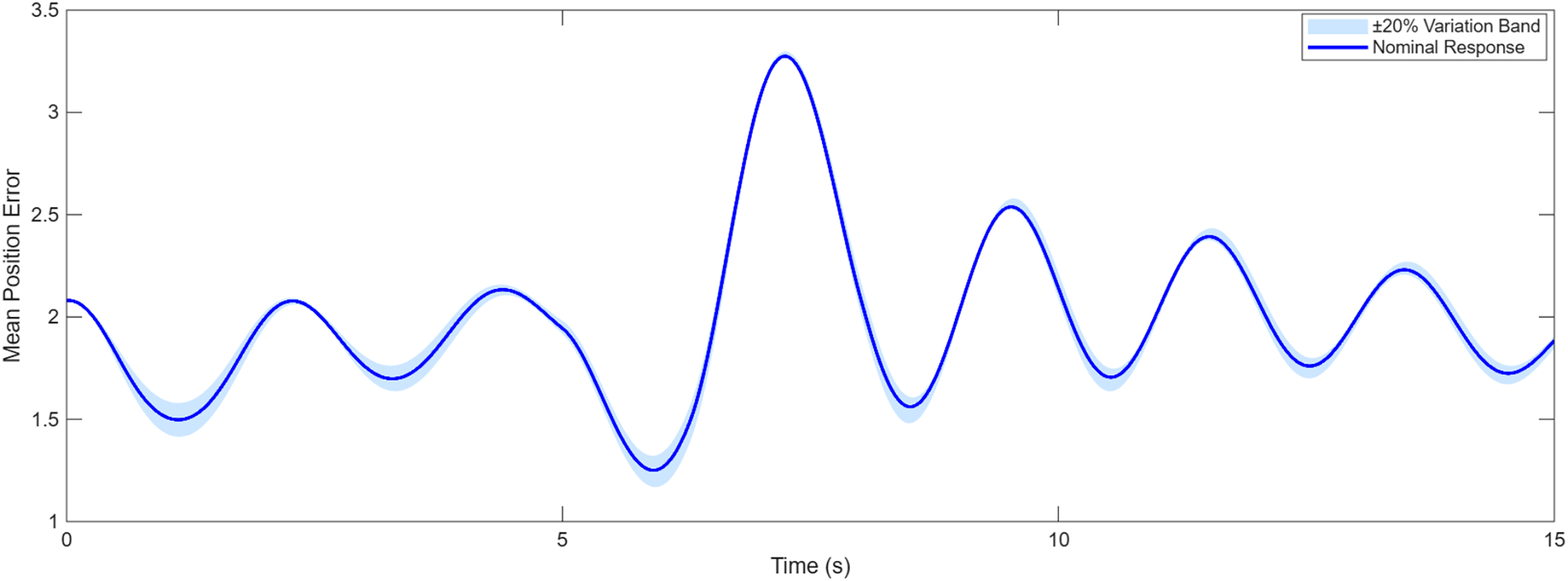
Figures 17 and 18 present the sensitivity analysis of the proposed RGT2FNN–SMC controller under 20% variations in key parameters, including the sliding gain, learning rate, and adaptation coefficient. The shaded regions indicate the performance range under these perturbations, while the solid curve represents the nominal response. The minimal spread of the shadow bands confirms that the controller maintains stable and consistent tracking accuracy, demonstrating low sensitivity to parameter tuning and high adaptability under model and design uncertainties. The proposed hybrid RGT2FNN–SMC framework also exhibits strong scalability potential for real-world applications. Since the control strategy is fully distributed, each agent requires only local neighbor information, which minimizes communication overhead as the network size increases. Furthermore, the RGT2FNN based adaptive estimator operates with low computational complexity, making real-time implementation feasible even in embedded processors or UAV swarms. These characteristics suggest that the proposed approach can be efficiently deployed in large-scale multi-agent systems operating under uncertain and dynamic environments.
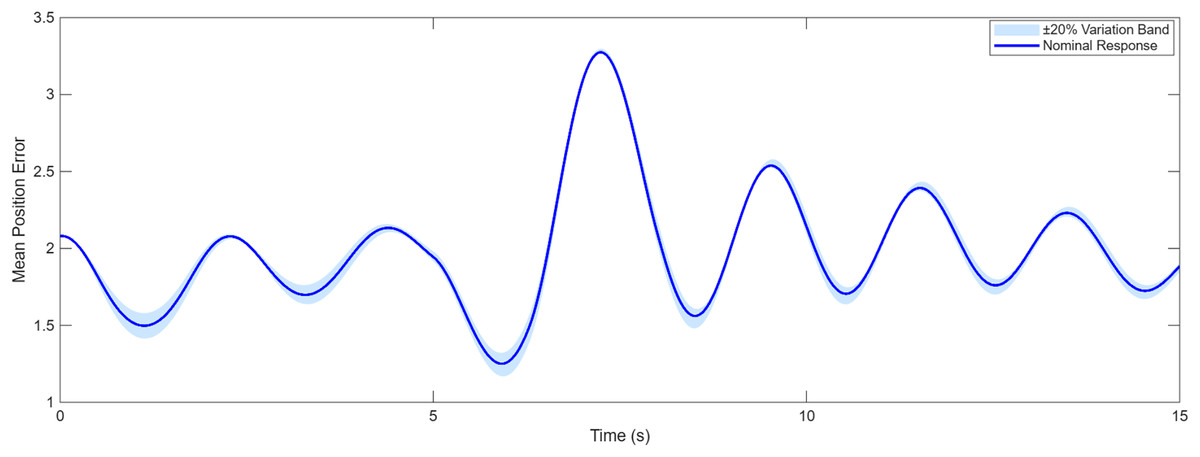
Figure 17: Sensitivity of position tracking under ±20% parameter variation in the RGT2FNN–SMC controller.
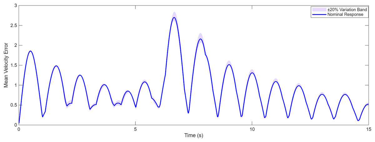
Figure 18: Sensitivity of velocity tracking under ±20% parameter variation in the RGT2FNN–SMC controller.
The proposed hybrid RGT2FNN–SMC framework also exhibits strong scalability potential for real-world applications. Since the control strategy is fully distributed, each agent requires only local neighbor information, which minimizes communication overhead as the network size increases. Furthermore, the RGT2FNN based adaptive estimator operates with low computational complexity, making real-time implementation feasible even in embedded processors or UAV swarms. These characteristics suggest that the proposed approach can be efficiently deployed in large-scale multi-agent systems operating under uncertain and dynamic environments.
Conclusion
This study presented a novel RGT2FNN–SMC framework for robust formation control of second-order MASs under switching topologies and actuator input constraints. The proposed approach integrates adaptive fuzzy neural estimation with sliding mode control to effectively compensate for unknown nonlinear dynamics and external disturbances while ensuring finite-time convergence and smooth control effort. Unlike conventional IT2FNN–SMC schemes, the proposed RGT2FNN–SMC introduces a gradient-based adaptation mechanism that enhances learning efficiency and stability, enabling the controller to maintain precise formation tracking even under dynamic uncertainties and limited control authority.
Beyond demonstrating robustness, the work establishes a scalable and computationally efficient framework suitable for real-time applications such as cooperative UAVs, autonomous vehicles, and robotic swarms. Simulation studies under switching topologies, input saturation, and disturbance conditions validate the controller’s stability, adaptability, and resilience, confirming its potential for deployment in complex real-world environments. Future research will focus on implementing the proposed method in a hardware-in-the-loop or experimental multi-agent platform, and on extending the adaptive learning structure to support event-triggered communication for reduced network load and enhanced coordination efficiency.