
Improved bipartite plots of ecological networks using the k-core decomposition with the BipartGraph application
- Published
- Accepted
- Received
- Academic Editor
- José Manuel Galán
- Subject Areas
- Algorithms and Analysis of Algorithms, Data Mining and Machine Learning, Network Science and Online Social Networks, Visual Analytics
- Keywords
- Visualization, Graph theory, Bipartite network, Open-source software
- Copyright
- © 2026 Garcia-Algarra
- Licence
- This is an open access article distributed under the terms of the Creative Commons Attribution License, which permits unrestricted use, distribution, reproduction and adaptation in any medium and for any purpose provided that it is properly attributed. For attribution, the original author(s), title, publication source (PeerJ Computer Science) and either DOI or URL of the article must be cited.
- Cite this article
- 2026. Improved bipartite plots of ecological networks using the k-core decomposition with the BipartGraph application. PeerJ Computer Science 12:e3526 https://doi.org/10.7717/peerj-cs.3526
Abstract
Visualizing bipartite networks with the well-known bipartite plot often produces an obfuscated image. This article introduces an approach that uses a two-pronged strategy to improve the readability of conventional bipartite plots. First, it reorders the network layout based on the k-core decomposition, positioning the central species more prominently. Second, it reduces visual clutter by grouping and compactly representing peripheral nodes. The new plotting feature is integrated into the open-source R package kcorebip and is also offered in the interactive web application BipartGraph. We explain the advantages of this innovation through several representative use cases showcasing its ability to generate clearer, more interpretable visualizations.
Introduction
Visualization is a powerful tool. Graphs, charts, and diagrams provide distilled information to researchers. It also simplifies the communication of complex data concepts, thereby improving comprehension and engagement for readers. As Edward R. Tufte wrote, there is a direct link between visual clarity and intellectual rigor (Tufte & Graves-Morris, 1983). Compelling visualizations reveal patterns, anomalies, and relationships that could otherwise remain unnoticed. Despite this fact, cluttered plots are not uncommon in literature, even if they do not provide helpful information.
Visualization is essential for network science (Kershenbaum & Murray, 2005; Brandes, Kenis & Raab, 2006; Pocock et al., 2016). A network is a set of nodes and links; a graph in mathematical language. The value of its structure cannot be ignored, as it supports some emerging network properties. Visualization connects raw data to intuitive understanding, facilitating exploratory analysis and the discovery of insights.
Networks naturally represent interactions in ecology (Bascompte, 2007; Bascompte & Jordano, 2007; Harvey et al., 2017), although the question of the conditions for the validity of network analysis remains an ongoing discussion. For instance, the relationships in a plant-pollinator community are more similar to those in a human social network than to the flow of electricity in a power grid or the movement of passengers in a public transit system. Therefore, magnitudes associated with material flows or fault propagation might be meaningless (Dormann, 2023). They are also useful for assessing stability and understanding co-evolutionary dynamics (Landi et al., 2018; Perc et al., 2013). A typical pattern in ecology involves two types of participants (prey/predator, plant/pollinator, host/parasite); thus, bipartite networks are widespread in this field (Delmas et al., 2019). There are two guilds, with each node representing one species. Thus, a binary bipartite network consists of nodes representing species from two distinct classes within a given community. A link shows interaction between two species. We use the expression interaction matrix in this work to describe a compact representation of bipartite networks as a matrix; each row represents a species from one guild and each column a species from the other guild. It is functionally equivalent to the adjacency matrix in graph theory. Still, all nodes, regardless of their guild, are represented as rows and columns in the latter, so it is always a square matrix, while the former is rectangular. The network is weighted when the link conveys a measure of the interaction strength. For instance, if the field team counts the number of visits of pollinators of species i to flowers of species j, and not only the presence or absence, the i,j element of the interaction matrix stores that value. The network is binary if they only record the interaction as a 1 value.
This article uses examples of three types of bipartite networks: pollination, seed dispersal, and parasitism. Despite their diverse nature, they share a typical pattern of large-degree generalist species and small-degree specialist species, connected to generalists but rarely to other specialists (Montoya, Pimm & Solé, 2006; Krishna et al., 2008; Staniczenko, Kopp & Allesina, 2013). The group of the most connected generalists is referred to as the network nucleus or network core.
Visual inspection is not the most reliable method for detecting specialization. Specialists in ecological networks may often represent poorly sampled animal species. In frugivory networks, specialist frugivores are generally represented by animal species with a minor fraction of fruits in their diets (Fricke et al., 2017). This fact, shared by any network visualization method in this field, may be taken into account by the researcher. To quantify specialization, we must calculate more sophisticated statistical measures such as nestedness and modularity, and compare the results of the empirical network with its null models to avoid the effects of pure randomness (Ulrich & Gotelli, 2007). Visual inspection is just a quick tool for initial exploration compared to these methods.
The familiar bipartite plot comprises two parallel sets of nodes, one for each guild, sorted in descending order of degree. Links are straight lines that connect pairs of interacting species. For weighted networks, the width of each link is a function of the observed interaction magnitude. This layout provides an intuitive view of the structure; however, the plot becomes cluttered beyond a certain number of nodes and links. In network visualization parlance, it turns into a hairball (Longabaugh, 2012; Nocaj, Ortmann & Brandes, 2014).
The most popular software tool for creating bipartite plots is the R bipartite package, which is a de facto standard among researchers (Dormann, Gruber & Fründ, 2008). It provides a robust set of functions for network analysis. Although it is not visualization-oriented software, it supports plots for binary and weighted data interactions. The equivalent package in Python is NetworkX (Hagberg, Swart & Schult, 2008). It provides functionality for constructing and analyzing bipartite graphs and offers basic drawing capabilities through the package matplotlib.
There are attractive examples of clear and informative bipartite plots in the literature, but counterexamples are not uncommon. Published messy plots result from the inherent shortcomings of bipartite plots, not from a lack of user expertise. Although it is a two-dimensional representation, nodes are arranged in a single dimension according to convention. Ordering by degree may seem like the natural choice to maintain some sense of network hierarchy, but degree is not an accurate proxy for centrality in the bipartite world (Faust, 1997; Duxbury, 2020). A node with a degree of 1 could be directly connected to the most central node or be part of a peripheral chain of specialists. Arranging nodes alphabetically by their species’ names is not a better choice.
The alternative to the bipartite diagram is the matrix plot, in which the nodes of both guilds are arranged in rows and columns. If a link exists between two species, the corresponding position in the matrix is filled with a solid color or a gradient if the network is weighted; otherwise, it remains empty. The matrix plot enjoys the advantage of two spatial dimensions but has shortcomings, such as visually detecting subtle structures.
To overcome the limitations of the bipartite diagram, we designed a new type of visualization called the ziggurat plot (Garcia-Algarra et al., 2018). This representation departed from the linear arrangement of the nodes, using an intrinsic property of graph connectivity known as k-core structure. The k-core of a network is defined as the largest subgraph in which every vertex is connected to at least k other vertices within that same subgraph (Seidman, 1983). It is a recursive concept; a 3-core species of guild A has at least 3 links to species of guild B, which, in turn, have 3 or more links to species of guild A. The k-core structure helps identify the most strongly connected group within the network: those species that share the maximum k index (often referred to as ). This structure highlights the most important interactions for the community’s function.
The ziggurat diagram offers several advantages over the bipartite, although the latter’s use is well-established in the research community. Therefore, when designing a new version of the visualization application BipartGraph, the aim was to enhance the bipartite plot by incorporating specific properties of the ziggurat diagram, albeit with a subtle aesthetic modification. To achieve this goal, we have employed the same two-pronged strategy that created the ziggurat diagram: spatial arrangement based on the k-core structure and reduction of visual information at peripheral nodes.
This work presents two improved variants of the bipartite plot, along with free, open-source software to create them, either by coding with the R package kcorebip or through an intuitive, interactive interface application: BipartGraph. It operates on any mainstream operating system and is easily installed as a Docker image. First, we summarize the k-core meaning in bipartite networks; then, we provide examples of applications for four bipartite interaction networks.
Methods
The k-core decomposition of bipartite networks
The k-core is a concept from graph theory that refers to a maximal subgraph in which each vertex has at least degree k, meaning it is connected to at least k other vertices within that subgraph (Dorogovtsev, Goltsev & Mendes, 2006; Kong et al., 2019). The maximal subgraph of degree k is the subset of all nodes that satisfy this condition, regardless of how many links its members have with nodes outside the subgraph. For instance, a node may have a high degree with links to nodes of degree 1. Those links are irrelevant if the node belongs to the 2-core. Seidman developed the simple pruning algorithm to classify network nodes according to the k-core to which they belong. It is a recursive procedure that removes nodes with a degree of or less (the initial value of k is 1). Continue removing nodes from the remaining graph with a degree smaller than k until all nodes meet the minimum required degree of k; that subset is the k-core. The maximum k-core value occurs when there are no nodes with a degree of in the remaining subset. Refer to Fig. 1 for a toy decomposition example.
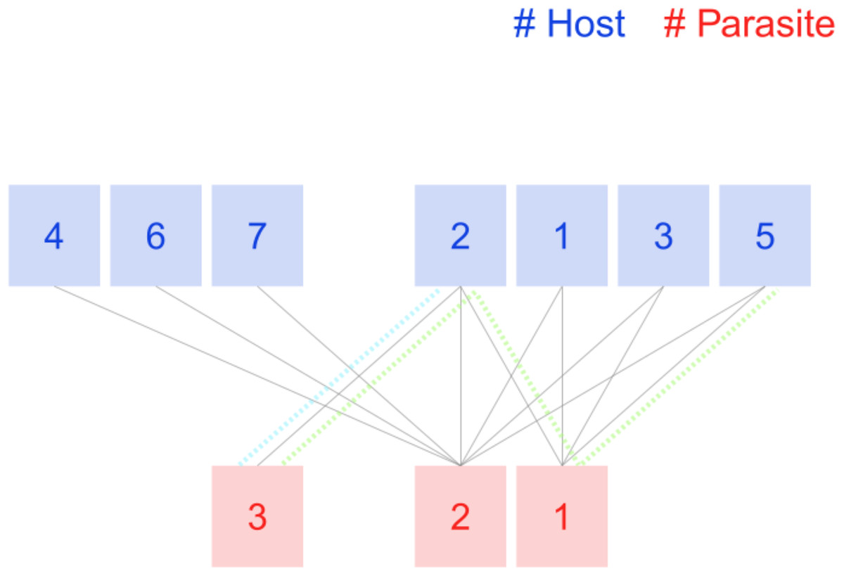
Figure 1: Tiny host-parasite host described in Hadfield et al. (2014).
Host nodes 4, 6, 7, and the parasite node 3 belong to the 1-shell because their degree is 1. The rest of the host nodes, including node 2, will keep only two links when the 1-shell is removed. Remove now those host nodes, and the remaining parasite nodes (2 and 1) get isolated, so is the maximum number for this network. Colored dotted lines are not part of the plot; we include them to explain the computation of magnitudes in Table 1.
| Species | Label | ||
|---|---|---|---|
| Amalaraeus penicilliger | Host 1 | 1 | 2 |
| Amphipsylla marikovskii | Host 2 | 1 | 2.4 |
| Catallagia dacenkoi | Host 3 | 1 | 2 |
| Hystrichopsylla microti | Host 4 | 2 | 1 |
| Megabothris advenarius | Host 5 | 1 | 2 |
| Rhadinopsylla integella | Host 6 | 2 | 1 |
| Stenoponia montana | Host 7 | 2 | 1 |
| Clethrionomys rufocanus | Parasite 1 | 1 | 4 |
| Clethrionomys rutilus | Parasite 2 | 1 | 5.5 |
| Microtus oeconomus | Parasite 3 | 2.5 | 1 |
All nodes belonging to the 3-core also belong to the 2-core because they have a degree of at least 2. Working with a related concept, the k-shell, proves convenient for practical purposes (Carmi et al., 2007). Nodes that belong to j-core but not to j+1-core constitute the k-shell. In the example, the nodes of 2-core that are not part of 3-core make up the 2-shell. For a node belonging to m-shell, the m index is referred to as its shell number or coreness.
The k-core decomposition groups nodes by their connectivity properties (Batagelj & Zaversnik, 2003), and is also valid for bipartite networks with a minor caveat. By definition, there must be nodes from both guilds in its maximum k-core because in bipartite networks, the degree counts the number of links to the opposite guild. So if equals 4, all nodes of guild A that belong to it have 4 or more links to species of guild B that have at least degree 4. However, that balance is not guaranteed for the rest of the k-shells. You may find networks with some k-shells consisting of nodes from just one guild.
Each node of the m-shell is linked to at least m other nodes within the same core. The innermost shell comprises the set of nodes with index . Nodes that exhibit higher degrees are called the generalists. In particular, nodes of the shell provide resilience to mutualistic communities when facing external perturbations (Bascompte & Jordano, 2007; Bastolla et al., 2009; Thébault & Fontaine, 2010). They also exhibit a nested connection pattern, where specialist species have a higher affinity for connecting with generalists than other specialists (Mariani et al., 2019). This empirical observation is quite helpful in improving bipartite plots, as described in this article. As coreness decreases, nodes become more specialized, while generalist nodes belong to higher k-shells.
Based on the k-core decomposition, we defined a unitless magnitude that serves as the foundation for our plots (Garcia-Algarra et al., 2017). The of node i of guild A (set ) is the average shortest path towards the nodes of the shell of guild B (set ).
(1)
The is a measure of distance to the shell. Its minimum possible value is 1 for a node in the shell that is directly linked to all nodes of the other guild belonging to the shell. This magnitude offers a natural way to represent the spatial distribution of nodes. It gives a hint about vulnerability, as a large indicates that the path to the central set of species is not direct. The act as a topological invariant that constrains the dynamic interaction strength between species, making it a condition for the stability of a system. The system may reach a critical point of collapse when the species belonging to the largest shell go extinct due to weakening interaction strength.
We define a second metric called , which is the sum of the reciprocals of the of neighboring nodes:
(2)
is the element of the interaction matrix considered as binary ( if , if ). We use as a secondary magnitude to resolve order ties when multiple nodes share the same value. It is a weighted degree; the connection to a central node is more valuable than to a peripheral node. provides a measure of average proximity to top generalists of the partner guild. Therefore, it may also act as a proxy for vulnerability, as eccentric species are more prone to becoming disconnected from the giant component.
Table 1 presents the values of both magnitudes for the example network. The 2-shell is a bipartite complete graph, so the k-radius is 1 for all its nodes. Parasite species 3 is tied to host species 2 (dotted blue line in Fig. 1), so the shortest path between them is 1. The shortest path from parasite 3 to host nodes 1, 3, and 5 is 3 (green dotted line in Fig. 1 is the path from it to host species 5). The k-radius of parasite node 3 is the mean of the four shortest paths, thus 2.5. Its k-degree is 1 as the sum of the reciprocals of the k-radius of neighboring nodes (host 2, k-radius 1). Unlike k-radius, which only takes into account shortest paths towards the shell, k-degree computation includes all neighboring nodes. Consider the difference between host species 2 and its peers of 2-shell. They all have two links with both nodes of parasite species of 2-shell. Node 2 has an additional link with parasite node 3, so its k-degree is 2.4, while the other host nodes 1, 3, and 5, have no links outside 2-shell and their k-degree is lower, just 2.0. Parasite 2 is linked to all host nodes and enjoys the highest k-degree of the network, 5.5.
We conducted a thorough comparison of the performance of k-core magnitudes vs degree and eigenvector centrality as measures of centrality in the context of network collapse, as defined in (Garcia-Algarra et al., 2017). The k-structure of the network is thus an estimator of resilience. It provides information about the global connection of the surviving nodes but not on how well-connected they remain after a shock, as another related magnitude from graph theory, the g–Good-Neighbor (Wang et al., 2024; Xiang & Hsieh, 2025).
The kcoreorder and chilopod plots
The k-core measure offers a natural method to organize the nodes, enhancing the readability of the legacy bipartite plot with minor modifications. To explain how it works, we have chosen a recent and well-documented example of a pollination network, in the natural reserve of Fiumedinisi and Monte Scuderi, Sicily (Italy) (Polidori et al., 2025). There are 33 species of plants and eight species of pollinators, all belonging to the genus Bombus. The network comprises 68 links, with the weight representing the number of captured and molecular barcode-identified pollinator individuals (289 in total). Plant species identification was conducted in situ. The authors published the interaction matrix as supplementary information.
It is a medium-sized network that exhibits typical features of pollination networks from a topological perspective. Figure 2A is the legacy bipartite plot of this community. Nodes are arranged in descending order of degree from left to right, and the width of each link corresponds to the square root of its weight. Detecting fine-grain structures is nearly impossible. For instance, the links among the most connected generalists and specialists on the right side are challenging to follow with the naked eye.
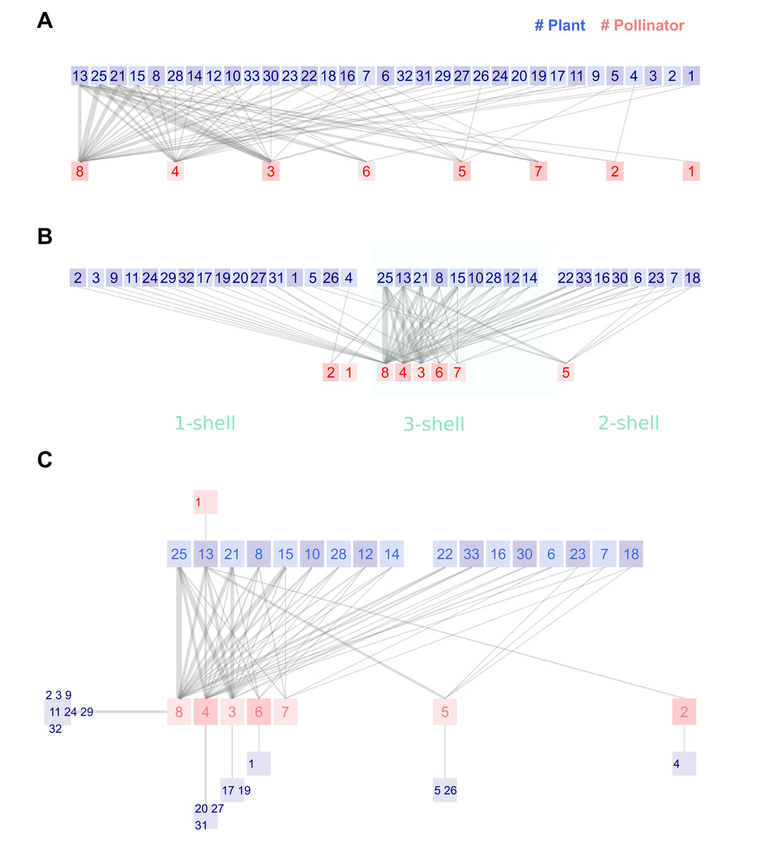
Figure 2: Legacy (A), kcoreorder (B) and chilopod (C) plots of a Bombus pollination network in the natural reserve of Fiumedinisi and Monte Scuderi, Sicily (Italy) (Polidori et al., 2025).
Pollinators: 1 Bombus campestris, 2 Bombus hortorum, 3 Bombus lapidarius, 4 Bombus pascuorum, 5 Bombus pratorum, 6 Bombus ruderatus, 7 Bombus sylvarum, 8 Bombus terrestris. Plants: 1 Acanthus mollis, 2 Anchusella cretica, 3 Asphodelus microcarpus, 4 Bituminaria bituminosa, 5 Borago officinalis, 6 Calamintha nepeta, 7 Carduus pycnocephalus, 8 Carlina hispanica, 9 Cirsium creticum, 10 Crepis leontodontoides, 11 Echium plantagineum, 12 Fedia graciliflora, 13 Galactites tomentosa, 14 Hirschfeldia incana, 15 Hypericum hircinum, 16 Hypericum perforatum, 17 Isatis tinctoria, 18 Lamium flexuosum, 19 Malva silvestris, 20 Micromeria canescens, 21 Onopordum illyricum, 22 Papaver rhoeas, 23 Ranunculus bulbosus, 24 Robia peregrina, 25 Rubus ulmifolius, 26 Silene latifolia, 27 Sixalix atropurpurea, 28 Taraxacum officinale, 29 Thapsia garganica, 30 Trifolium incarnatum, 31 Trifolium pratense, 32 Verbascum pulverulentum, 33 Vicia villosa.
The first enhanced variant is the kcoreorder plot (Fig. 2B). The procedure begins by plotting the shell at the center of the canvas. Bombus terrestris and Rubus ulmifolius are the most central species of each guild, both with the minimum possible k-radius value 1. Nodes are ordered by ascending k-radius. When two nodes have the same k-radius, the k-degree is used as a secondary criterion to break ties. Bombus ruderatus and Bombus sylvarum (nodes 6 and 7) share the same k-radius 2.33, but Bombus ruderatus’ k-degree is higher so it lays closer to Bombus terrestris. A small blank space, the size of one node, separates 2-shell from 3-shell. Again, nodes are sorted by ascending k-radius and descending k-degree. We have labeled the shells in Fig. 2B, with a softly colored background that is not present in the actual plots. The idea is that the visual distance to the central node correlates with k-radius. Finally, the nodes of 1-shell are displayed on the left of the shell. Most of them have links only towards nodes in the maximum shell, and this organization minimizes their lengths, which is one of the issues with the legacy plot.
The kcoreorder plot does not reduce visual information; it merely reorders the positions of nodes and, on average, shortens the length of links. The second step of the strategy involves shifting the peripheral nodes outside the bilinear section of the plot. In addition, we reduce information by clustering species that have only one link to a common partner. The result is the chilopod plot, named for its resemblance to a centipede in larger networks. Figure 2C is the chilopod plot of the Sicilian network. Shells 3 and 2 are displayed as in the kcoreorder plot. However, reorganizing the nodes of the 1-shell yields a clearer image.
The clusters of specialists connected to central species effectively reduce the number of visual nodes. Comparing the reduction of noise around pollinators of 3-shell, it is now easy to discover connections. Moreover, the chilopod reveals hidden details. Notice the chain of specialists that connects plant13-pollinator2-plant4. The k-radius of the last species is 3.4, while that for another specialist, plant1, tied to the shell, is 2.6. The position of pollinator species 5 is also interesting. It has only one link to 3-shell, but three with nodes of 2-shell, in addition to links with two 1-shell specialists. If this species is removed, plants 5 and 26 will become isolated. Plant species 13 plays a critical role, as the unique pollen source for bumblebees of species 1 and is the root node of the chain of specialists pollinator 2-plant 4. The extinction of this species would significantly affect the network structure.
Data
The BipartGraph dataset is mainly based on the Web of life collection (http://www.web-of-life.es/) (Fortuna, Ortega & Bascompte, 2014). The application offers over 100 mutualistic communities and 51 host-parasite networks available for download from the site. We preprocess the parasitic network files to remove the sum of interactions. We have incorporated a small number of datasets from other sources for the use cases of this study. Network sizes range from 6 to 431 species. We display species names as they appear in the original files, even when they are incomplete or imprecise.
Software implementation
The three variants of the bipartite plot are a new function bipartite_graph() of the R package kcorebip, which is distributed under an open-source MIT license. We utilize the function coreness from the package igraph to perform the k-core decomposition (Csardi & Nepusz, 2006).
The plotting algorithm is an original development that creates the image in two different formats: as a ggplot2 object (Wickham, 2011), and as a Scalable Vector Graphics (SVG) object. The user can save the plot as a file, but the ggplot2 object can be modified after invocation.
The function has 31 input parameters, and its syntax can be daunting for users. This issue is common among other plotting packages. The final appearance of a plot relies on many small adjustments. Users are often unwilling to invest their time in mastering an obscure function just to produce print-ready files for a paper or presentation.
We developed an interactive web application, BipartGraph, to break this barrier. Instead of saving the ggplot2 object, BipartGraph displays the SVG version within a user-friendly web application. The user can browse, zoom, and modify the final aspect of the network without any coding. Simply uploading the interaction matrix in .csv format is sufficient to create one of the four types of plots that the application offers: the three variants of bipartite plot, ziggurat, matrix, and polar.
When the plot is ready for publishing, the user can save the configuration parameters as a text file for future use. Moreover, if there is a need to reproduce plots within a more complex R script, BipartGraph exports as a text file, as well, the function call with the user’s settings modified through the user interface.
The interactive layer of BipartGraph combines the native features of the R Shiny package (Chang et al., 2025) with custom JavaScript code.
The installation and deployment of BipartGraph is available as a native R application and as a Docker image. Refer to the Software Availability subsection for details.
Results
The first example is an ant-plant symbiotic community in Mexico (Dáttilo, Díaz-Castelazo & Rico-Gray, 2014). These ant species feed on extrafloral nectar and offer defense against herbivores. There are ant species, plant species, and links, so it is a balanced and medium-sized network. The authors recorded weighted observations but included a classical binary bipartite plot, so clean that we could visually reproduce the interaction matrix.
We present the three possible flavors of the bipartite plot in Fig. 3. The legacy bipartite follows the sequence of the original study, with species of higher degrees positioned on the left side. An experienced researcher may gain some insight from the graph. However, discovering structural details remains challenging, even for a network of this size.
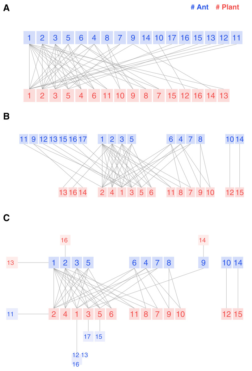
Figure 3: Legacy (A), kcoreorder (B) and chilopod (C) bipartite plots of an ant-plant network in Mexico (Dáttilo, Díaz-Castelazo & Rico-Gray, 2014).
Ants: 1 Forelius pruinosus, 2 Camponotus planatus, 3 Monomorium ebeninum, 4 Cephalotes minutus, 5 Dorymyrmex bicolor, 6 Paratrechina longicornis, 7 Crematogaster obscurata, 8 Pseudomyrmex oculatus, 9 Camponotus mucronatus, 10 Camponotus novogradensis, 11 Crematogaster crinosa, 12 Crematogaster rochai, 13 Crematogaster torosa, 14 Monomorium floricola, 15 Pseudomyrmex gracilis, 16 Pseudomyrmex pallidus, 17 Solepnosis geminata. Plants: 1 Opuntia sctricta, 2 Macroptilium atropupureum, 3 Mansoa hymenaea, 4 Crotolaria incana, 5 Cedrela odorata, 6 Chamaecrista chamecristoides, 7 Caesalpinia crista, 8 Canavalia rosea, 9 Petrea volubilis, 10 Prestonia mexicana, 11 Turnera ulmifolia, 12 Capparis baduca, 13 Ipomoea pres-caprae, 14 Passiflora sp, 15 Serjania sp, 16 Terminalia catappa.
The structure reveals itself in the kcoreorder plot. For instance, the four species on the figure’s right side are disconnected from the network’s giant component. Their k-radius is infinite, and there is no path to reach the central species of 3-shell. Another interesting fact about this community is that the specialists of 1-shell, plotted on the left edge, interact with species of 3-shell, but none of them interact with species of 2-shell. That is a hint of strong nestedness.
Finally, the chilopod plot provides additional visual insights and is more readable. Ant specialists feed on 3-shell plants. Opuntia stricta (plant 1) is not the most central species because, despite its higher degree, it is less connected to 3-core ant species than Macroptilium atropupureum. There is also a chain of specialists , which is difficult to discover in the previous plot variants. Ant species 6 and 8 share the 2-shell number, but their k-radius (2.33 vs 4.33) shows that the first one is well connected to central plant species, while the second one is peripheral.
The study’s research question was whether competition among ant species drives the shape of the network. We can read in the discussion section: Here we show that although ants have an extremely territorial effect only near their nests, competition among ants is intense enough to structure ant–plant networks. Specifically, we show that ant’s position within the nested ant–plant network can be predicted only by differences among ant species’ competitive ability (numerical dominance and recruitment). The study identifies three ant species as the most significant competitive: Forelius pruinosus, Camponotus planatus and Monomorium ebeninum that happen to be nodes with labels 1, 2 and 3 in Fig. 3C. Their feeding habits include the plant central species Opuntia stricta, Macroptilium atropurpureum, and Mansoa hymenaea, which belong as well, to the max k-shell. So, according to this conclusion, there is a gradient of competitiveness among ant species, and their k-radius correlates with that behavior.
Moving on to weighted networks, we analyze the Safariland dataset (Vázquez & Simberloff, 2003). This small pollination community in Argentina is somewhat the hello world of network visualization, as the popular plotweb function of the bipartite package uses it as an example. The original research compared eight different sites in Nahuel Hapi National Park (Argentina)—four grazed and four ungrazed—to determine if the human introduction of ungulates affects pollination networks. One of the sites is Safariland, where no cattle could disturb the natural pollination community.
Figure 4A is nearly the default outcome of applying plotweb to the dataset; we have made slight adjustments for improved readability. The function offers numerous input parameters to customize the graph; however, as we explained, non-expert users may feel overwhelmed and use the default values instead. The width of each link corresponds to the numerical value recorded in the interaction matrix, which, for this study, was the quantity of observed interactions. The aesthetic effect is a visual predominance of the most active nodes like Aristotelia chilensis and Policana albopilosa. However, human visual perception is not linearly proportional to stimuli but to their logarithms, an observation known as Fechner’s Law (Algom, 2021). Vázquez and Simberloff plotted several snapshots of the network with link widths proportional to the square root of the interaction.
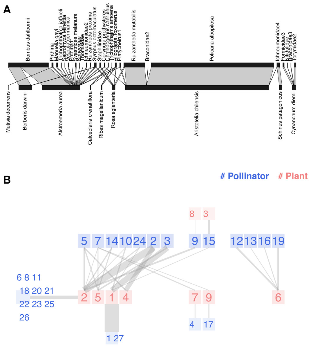
Figure 4: Two representations of the Safariland network (Vázquez & Simberloff, 2003): (A) using bipartite::plotweb function, (B) chilopod plot.
Pollinators: 1 Policana albopilosa, 2 Bombus dahlbomii, 3 Ruizantheda mutabilis, 4 Trichophthalma amoena, 5 Syrphus octomaculatus, 6 Manuelia gayi, 7 Allograpta Toxomerus, 8 Trichophthalma jaffueli, 9 Phthiria, 10 Platycheirus1, 11 Sapromyza Minettia, 12 Formicidae3, 13 Nitidulidae, 14 Staphilinidae, 15 Ichneumonidae4, 16 Braconidae3, 17 Chalepogenus caeruleus, 18 Vespula germanica, 19 Torymidae2, 20 Phthiria1, 21 Svastrides melanura, 22 Sphecidae, 23 Thomisidae, 24 Corynura prothysteres, 25 Ichneumonidae2, 26 Ruizantheda proxima, 27 Braconidae2. Plants: 1 Aristotelia chilensis, 2 Alstroemeria aurea, 3 Schinus patagonicus, 4 Berberis darwinii, 5 Rosa eglanteria, 6 Cynanchum diemii, 7 Ribes magellanicum, 8 Mutisia decurrens, 9 Calceolaria crenatiflora.
Figure 4B presents the chilopod plot of Safariland. Following the original paper’s approach, link widths are proportional to the square root of interactions and semi-transparent to reduce eye strain. When several peripheral nodes share connections with a central node, we sum the interactions before computing the square root. The chilopod reveals some interesting facts. Policana albopilosa is a peripheral species, while Syrphus octomaculatus is the most generalist and central pollinator species according to its k-core number. The chains of specialists are easy to spot in the center of the image, as well as the disconnected subnetwork on the right.
An isolated plot is insufficient to evaluate the value of visualization in addressing this research question; you should compare the chilopod diagrams from the eight sites, as the authors did with traditional bipartite plots. While it is beyond the scope of this paper, some discussion details could be easily identified. The primary conclusion was that grazing disrupts the pollination network. For instance, as they observed: the herb Alstroemeria aurea interacts very frequently with the bumblebee Bombus dahlbomii in ungrazed sites, but it does so less frequently in grazed sites, where both species are relatively rare; conversely, the interaction between the understorey tree Schinus patagonicus and the halictid bee Ruizantheda mutabilis is frequent in grazed sites but virtually absent from ungrazed sites. The interaction of Alstroemeria aurea, the central plant species according to its k-radius, and Bombus dahlbomii is quite clear in Fig. 4. Schinus patagonicus is one of two plant species that only receives visits from one pollinator species that is not Ruizantheda mutabilis, which is part of the network nucleus.
The two networks described so far have a moderate size, with fewer than 50 links. Beyond that number, the traditional bipartite diagram becomes unreadable. In contrast, the chilopod remains functional for networks of up to a hundred links. The third case consists of a network of insects (Hymenoptera, Lepidoptera, Diptera, and Coleoptera) and flowering plants (Dicks, Corbet & Pywell, 2002), sampled at two locations throughout an entire season in Norfolk (UK). It has weighted links; their widths are plotted proportional to the natural logarithm of the number of recorded visits. Figure 5 shows the chilopod plot of this network in a vertical layout, with the most central nodes positioned at the top.
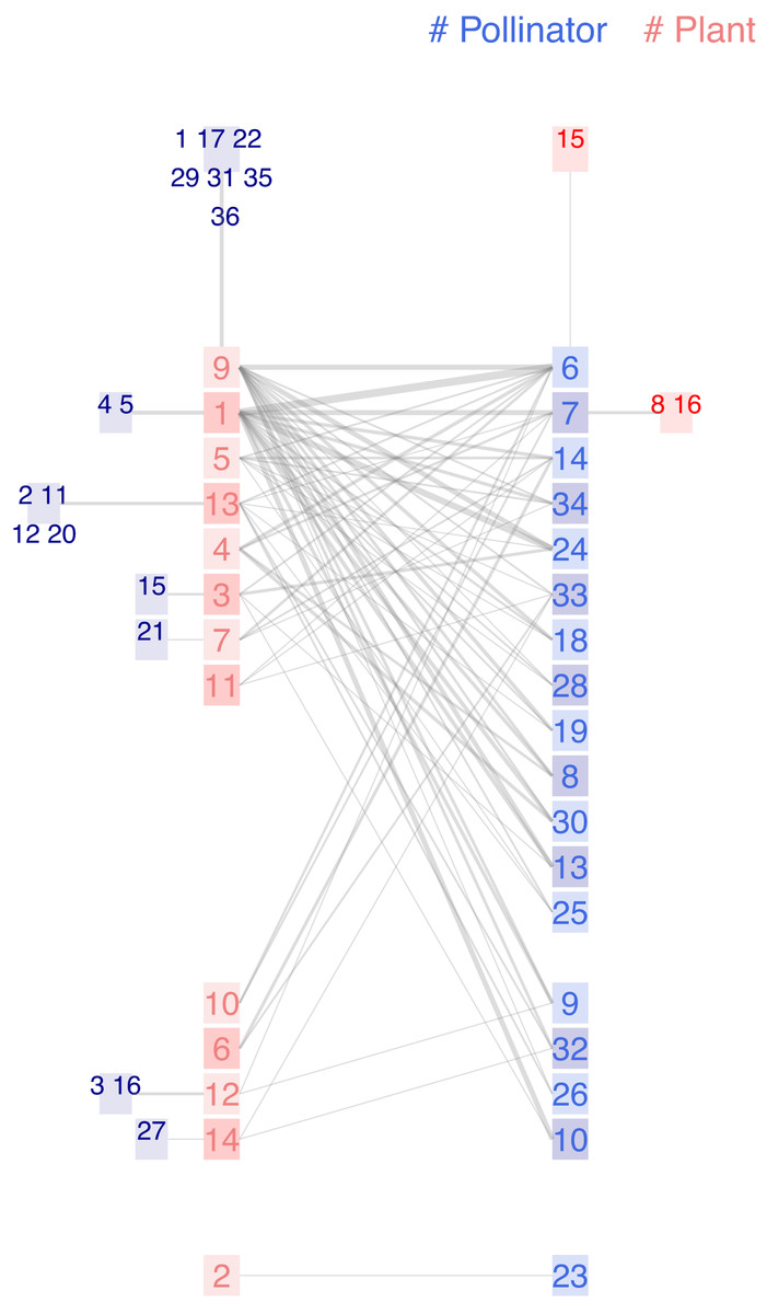
Figure 5: Chilopod plot a plant-pollinator mutualisitic network in Norfolk, UK (Dicks, Corbet & Pywell, 2002).
Pollinators: 1 Andrena chrysosceles, 2 Andrena pubescens, 3 Anthophora plumipes, 4 Apis mellifera, 5 Bombus hortorum, 6 Bombus lapidarius, 7 Bombus pascuorum, 8 Bombus pratorum, 9 Bombus terrestris lucorum, 10 Calocoris bipunctatus, 11 Cephus pygmaeus, 12 Cheilosia bergenstammi, 13 Empis livida, 14 Episyrphus balteatus, 15 Eriothrix rufomaculatus, 16 Eristalis intricarius, 17 Eristalis nemorum, 18 Eristalis tenax, 19 Helophilus sp1, 20 Lasioglossum calceatum, 21 Lasioglossum villosulum, 22 Lucillia sp1, 23 Lycaena phlaeas, 24 Maniola jurtina, 25 Melanostoma sp1, 26 Meliscaeva sp1, 27 Panameria tenebrata, 28 Platycheirus sp1, 29 Pollenia sp1, 30 Psithyrus vest, 31 Sarcophagus sp1, 32 Scathophaga stercoraria, 33 Sphaerophoria sp1, 34 Syrphus sp1, 35 Tropidia scitta, 36 Volucella bombylans. Plants: 1 Centaurea nigra, 2 Cerastium fontanum, 3 Cirsium arvense, 4 Cirsium palustre, 5 Filipendula ulmaria, 6 Galium verum, 7 Hypochoeris radicata, 8 Lathyrus pratensis, 9 Leucanthemum vulgare, 10 Lotus corniculatus, 11 Orchis morio, 12 Primula veris, 13 Ranunculus acris, 14 Taraxacum officinale, 15 Trifolium dubium, 16 Trifolium repens.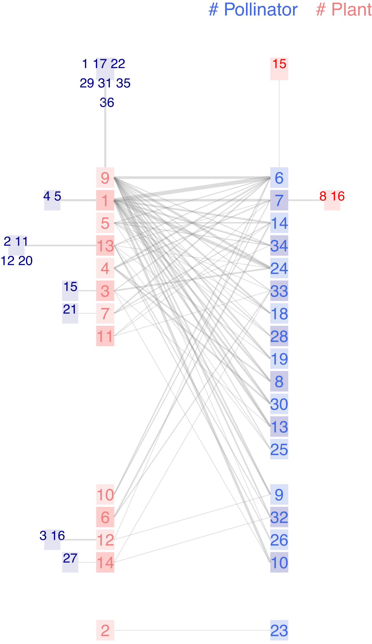
This research aimed to investigate compartmentalization, a type of analysis that goes beyond visual inspection. Nevertheless, the chilopod plot offers some insights into the network’s structure. Around half of insect species feed on just one type of plant, whereas plants tend to be more generalist. This was noted by the authors: There are invariably many more insect species than plant species, and most insects show a degree of generality in their foraging choice (Waser et al., 1996). As pointed out by Elberling & Olesen (1999), this leads to plant species having far more generalized interactions than the insect species in pollination webs. The three specialist plants Lathyrus pratensis, Trifolium dubium, and Trifolium repens belong to the family of Fabaceae and receive visits from two Bombus species. The exploratory analysis may provide additional insights for the expert user by utilizing the interactive interface.
The fourth and final example illustrates the limitations of the chilopod diagram, featuring a network of seed-dispersing frugivorous birds in a fragment of subtropical forest in Brazil (Galetti & Pizo, 1996). We include the proper citation to the original paper published in the Brazilian journal Ararajuba in 1996 because the date is relevant. In other sources, it is dated to 2013, when it appeared as part of a collection. The field study was conducted from 1988 to 1991, a time when network analysis was not as standard in ecology as it is today. The research team recorded 399 feeding bouts of 29 bird species, known for their role as seed dispersers, on 36 plant species within a 250 ha fragment of subtropical forest surrounded by an agricultural landscape. They published the observed feeding events as tabulated data. The descriptive study outlines foraging patterns and compatibility between seed and bird anatomy. It does not provide any plots or a network perspective.
The interaction matrix has 146 weighted links; each observed bout between a pair of bird and plant species adds 1 to the matrix. Although it is not a strict rule, as it depends on the total number of nodes and the balance between guilds, 150 links serves as the threshold that degrades the usefulness of the chilopod plot. It reduces the visual stress of the legacy plot by shifting specialists outside the central two-line set of nodes. As links increase, the space between guilds will eventually become cluttered. Surrounding specialists remain easy to spot in Fig. 4A, but the network core is evolving into the dreaded hairball. The interactive interface alleviates this problem as users can explore individual connections by clicking on a specific node; however, this is a reasonable limit for printed images.
We developed the ziggurat plot to handle larger-sized networks. As Fig. 6B shows, in the ziggurat, links among nodes that do not belong to the max k-shell lie outside the central and smaller bilinear plot. The downside is that nodes are not equally shaped or sized; this plotting method prevents links from crossing over nodes.
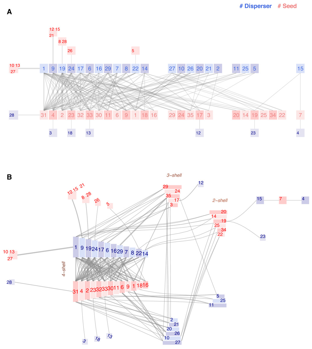
Figure 6: Chilopod (A) and ziggurat (B) plots of a frugivory network in Southeastern Brazil (Galetti & Pizo, 1996).
Dispersers: 1 Chiroxiphia caudata, 2 Coereba flaveola, 3 Conirostrum speciosum, 4 Cyanocorax cristatellus, 5 Cyclarhis gujanensis, 6 Dacnis cayana, 7 Elaenia flavogaster, 8 Habia rubica, 9 Manacus manacus, 10 Myiodynastes maculatus, 11 Myiophobus fasciatus, 12 Penelope superciliaris, 13 Pipraeidea melanonota, 14 Pitangus sulphuratus, 15 Ramphastos toco, 16 Ramphocelus carbo, 17 Saltator similis, 18 Sirystes sibilator, 19 Tachyphonus coronatus, 20 Tangara cayana, 21 Thlypopsis sordida, 22 Thraupis sayaca, 23 Tityra cayana, 24 Trichothraupis melanops, 25 Turdus amaurochalinus, 26 Turdus rufiventris, 27 Tyrannus melancholicus, 28 Tyrannus savanna, 29 Vireo olivaceus. Seeds: 1 Cabralea canjerana, 2 Cecropia pachystachia, 3 Cestrum sp1, 4 Chamissoa altissima, 5 Chlorophora tinctoria, 6 Citharexylum mirianthum, 7 Copaifera langsdorffii, 8 Cordia sp1, 9 Dendropanax cuneatum, 10 Ficus luschnatiana, 11 Gomidesia affinis, 12 Maytenus aquifolium, 13 Miconia discolor, 14 Miconia elegans, 15 Miconia sp1, 16 Momordica charantia, 17 Ocotea corimbosa, 18 Ocotea macropoda, 19 Ocotea sp1, 20 Palicourea sp1, 21 Paullinia rhomboidea, 22 Paullinia sp1, 23 Pera glabrata, 24 Pereskia aculeata, 25 Persia major, 26 Piper sp1, 27 Protium heptaphyllum, 28 Rhipsalis sp1, 29 Rubus sp1, 30 Talauma ovata, 31 Trema micrantha, 32 Trichilia clauseni, 33 Urera baccifera, 34 Xylopia brasiliensis, 35 Zanthoxylum hyemale.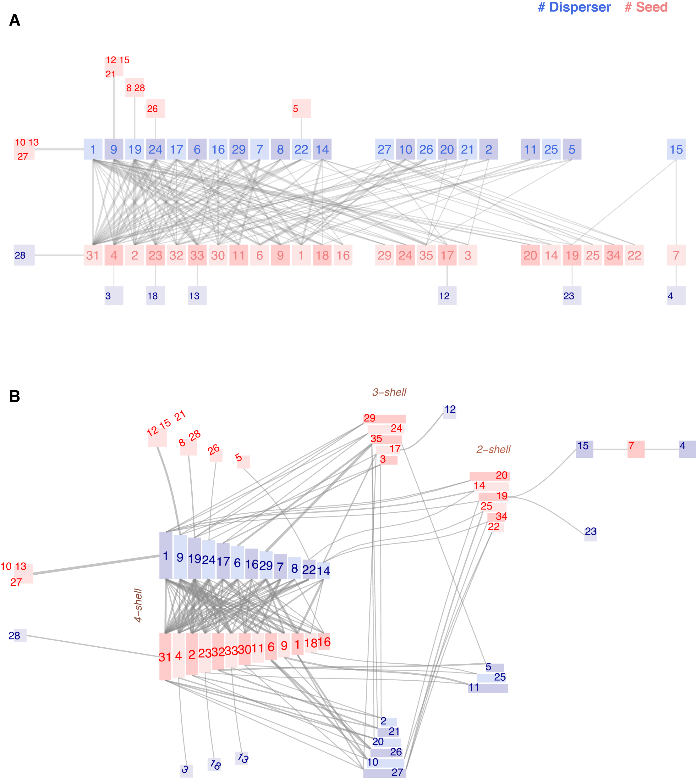
Galetti and Pizo’s central hypothesis is that forest fragments have a long-term impact on vegetation due to human activity disturbance: Large frugivorous birds may fail to subsist in fragmented areas where their food resources have diminished following unusual climatic conditions or logging, triggering a series of extinctions in a domino effect.
In the conclusions, we read that plants producing small seeds colonize fragmented areas, thereby attracting small passerines. The authors cite, as examples of abundant colonizers Trema micrantha and Cecropia pachystachia (labeled 31 and 2 in our plots), and also mention Camissoa altissima (label 4) as the primary fruit bearer in winter. Maybe coincidental, but they are the three species with higher k-radius. On the opposite side, they wrote that plant species with larger diaspores (>10 mm) invariably had a small feeding assemblage [ ..]. In the non-fragmented forest, many bird species ate the fruits of Capaifera langsdorffii. Still, they observed that, inside the isolated area they studied, only two species fed on it. Ramphastos toco and Cyanocorax cristatellus are big enough to swallow the seeds and belong to the group of threatened large frugivores. The chain is a striking detail visible in both plots (bird15-plant7-bird4). According to the study, the three species are endangered and occupy an ultra-peripheral position in the network, characterized by extreme k-radius values.
Conclusions
These findings show that the traditional bipartite visualization is boosted by utilizing the k-core decomposition. Grouping species by their coreness uncovers the hierarchy of connections and reduces the average link length, thus minimizing clutter. This is what we call the kcoreorder bipartite plot. Additionally, plotting specialists outside the bilinear group of central species and clustering those with the same partner in common nodes enhances readability. This variant is the chilopod bipartite plot. The width of each link is a function of its weight (square root, natural, or common logarithm), facilitating intuitive visual comparison of magnitudes.
Visualization is crucial during the exploratory analysis of networks (Slingsby & van Loon, 2016; Borcard et al., 2018). Plots help identify central species, chains of specialists, or nodes that do not fit into the characteristic nested pattern (Jordano, Bascompte & Olesen, 2006). Adjusting the plot through programming requires setting several parameters. This issue leads to suboptimal plots, where the program calls functions with default input values. Providing a user-friendly interactive application makes the tool usable for any end user, regardless of programming skills. It also offers publication-ready files and R code for reproducibility.
Through the discussion of four use cases, we conclude that the chilopod plot is compelling for bipartite networks with over 50 links, a practical limit for the legacy layout. It continues to function well with between 50 and 100 links, but its readability declines beyond 150, requiring a switch to an alternative plot type like the ziggurat. The chilopod functions when the degree distribution is heterogeneous, as seen in ecological bipartite networks. For a complete bipartite graph, all nodes belong to the shell and share the same degree. Thus, the chilopod would be identical to the legacy plot.
Although visualization is as helpful in ecology as in other applications of network science, there are few examples of plots tailored to ecological networks (Etemad, Carpendale & Samavati, 2014; Marzidovšek et al., 2022). Other life sciences disciplines have developed their visualization tools (Shannon et al., 2003; Letunic & Bork, 2007; Theocharidis et al., 2009), but ecology relies on standard plots. We have demonstrated how, by spatially arranging species according to their k-shell, the classical bipartite plot becomes more suitable for ecological networks.
Moreover, visualization tools must be as user-friendly as possible. There is no reason to develop a powerful tool that requires numerous configuration parameters to adjust, forcing users to never go beyond the default invocation. This lesson can be challenging for computer science teams to learn, but it is crucial for effective collaboration.