
From recursion to prediction: modeling backtracking effort in TSP with machine learning
- Published
- Accepted
- Received
- Academic Editor
- Massimiliano Fasi
- Subject Areas
- Algorithms and Analysis of Algorithms, Artificial Intelligence, Data Mining and Machine Learning, Optimization Theory and Computation, Scientific Computing and Simulation
- Keywords
- Backtracking algorithms, Computational cost prediction, Machine learning regression, Resource-aware optimization, Traveling salesman problem
- Copyright
- © 2026 Xie et al.
- Licence
- This is an open access article distributed under the terms of the Creative Commons Attribution License, which permits unrestricted use, distribution, reproduction and adaptation in any medium and for any purpose provided that it is properly attributed. For attribution, the original author(s), title, publication source (PeerJ Computer Science) and either DOI or URL of the article must be cited.
- Cite this article
- 2026. From recursion to prediction: modeling backtracking effort in TSP with machine learning. PeerJ Computer Science 12:e3516 https://doi.org/10.7717/peerj-cs.3516
Abstract
The Traveling Salesman Problem (TSP) is a well-known Nondeterministic Polynomial-time (NP)-hard problem in combinatorial optimization. Solving TSP instances optimally using backtracking algorithms guarantees accuracy but incurs significant computational costs, especially for medium-scale problems. Little attention has been given to predicting the computational workload of TSP solvers based on backtracking using artificial intelligence. The precise estimation of resource usage is a complex and challenging issue due to the high variability of heterogeneous optimization problems. This article proposes a method for predicting the computational cost of solving the TSP using a backtrack solver through a machine learning approach. We propose a machine learning framework for estimating the computational effort required to solve TSP instances using backtracking techniques. Synthetic datasets are generated where each instance includes engineered features. Supervised machine learning models are proposed, tuned, and evaluated using various methods to estimate the computational cost for the TSP accurately. Results illustrate that among the 12 machine learning models of different classes, the regression models perform better. These models achieve a predictive accuracy of 99%, demonstrating strong consistency with actual results. The results also validate the potential of artificial intelligence (AI), focusing on the computational demands of optimization problems like TSP. We propose a machine learning framework that can be applied to optimization problems for intelligent solver selection, runtime estimation, and resource-aware scheduling.
Introduction
Combinatorial optimization problems lie at the heart of numerous real-world applications in logistics, operations research, telecommunications, and transportation (Silva, Ribeiro & Gomes, 2023; Ali et al., 2016). As an NP-hard problem, the Traveling Salesman Problem (TSP) is among the most extensively studied and challenging. The computational effort needed to find the optimal solution increases exponentially with the number of cities. It is often impossible to solve TSP instances optimally using traditional algorithmic approaches, such as backtracking. In large, unrestricted solution spaces, it leads to resource inefficiencies and long execution times (Kool et al., 2022).
Machine learning (ML) has recently revolutionized combinatorial optimization, particularly in predicting computational workload in backtracking algorithms for the Traveling Salesman Problem (TSP) (Ahmad, 2025). This development has coincided with advances in traditional optimization methods. Machine learning excels in pattern recognition, predictive modeling, and adaptive behavior, making it a natural candidate for improving combinatorial optimization workflows. By learning from historical problem-solving data, machine learning models can predict algorithmic behavior, computational demands, and search strategies. This capability enables them to reduce unnecessary computations and boost efficiency without sacrificing effectiveness (Telikani et al., 2021). Combining traditional optimization and artificial Intelligence (AI) can predict solver workload and behavior without running the algorithm. The benefits include better resource planning, adaptive algorithm selection, and accurate runtime estimation. Using machine learning to forecast the computational workload of a backtracking-based solver is a novel approach to optimizing solver performance in the TSP, especially in resource-constrained environments. This research bridges the gap between algorithmic rigor and data-driven prediction models by combining combinatorial optimization with AI (Zhou et al., 2025).
Recent advancements in neural combinatorial optimization (NCO) have significantly enhanced solutions for routing and the TSP. Research conducted by Sui et al. (2025) and Alanzi & Menai (2025) offers comprehensive frameworks for learning-based TSP solvers, emphasizing generalizable neural models that outperform traditional heuristics. Scalable deep learning architectures, including Transformer-based models and graph neural networks such as LEHD (Wu et al., 2024) and GLOP (Ye et al., 2024), demonstrate adaptability to various problem sizes by including hierarchical and attention mechanisms. Furthermore, reinforcement learning-based non-autoregressive frameworks such as Graph-based Diffusion Solvers for Combinatorial Optimization (DIFUSCO) (Sun & Yang, 2023) and diffusion-based solvers (Wang et al., 2025) facilitate fast path finding through parallel inference and improved scalability. The incorporation of these improvements places the current study at the forefront of AI-driven combinatorial optimization.
Deep learning (DL) techniques can address the Traveling Salesman Problem (TSP) by deriving data-driven heuristics rather than relying on predefined rules. Graph Neural Networks (GNNs), Pointer Networks, and Transformers capture spatial and relational dynamics among nodes, facilitating scalable, near-optimal solutions for large datasets (Alanzi & Menai, 2025). Recent hybrid models that combine deep learning with classical methods, such as the Lin-Kernighan-Helsgaun (LKH) algorithm, improve solution quality and efficiency (Li, Tu & Xu, 2024). DRHG, LocalEscaper, and diffusion-based methods can manage tens of thousands of nodes and exhibit generalization (Li et al., 2025; Wen et al., 2025). The work (Lyu, Islam & Yu, 2024) introduces a scalable supervised learning technique for the TSP utilizing “anchors” to represent local node interactions. This strategy enhances accuracy and accelerates performance on extensive TSP situations by integrating these predictions with conventional solvers. Deep learning-based algorithms are adaptable, rapid, and of superior quality for complex combinatorial optimization tasks such as the TSP.
Deep learning for the Traveling Salesman Problem and vehicle routing encompasses three distinct yet complementary domains. Neural combinatorial optimization (NCO) for the vehicle routing problem (VRP) and the traveling salesman problem (TSP) substitutes manually designed rules with learn policies or components and can be integrated with exact solvers; for instance, a scalable learning-plus-integer linear programming (ILP) framework enhances the performance of large capacitated vehicle routing problems (CVRP) while maintaining feasibility and practical constraints (Fitzpatrick, Ajwani & Carroll, 2024). Scalable models that accommodate various sizes and distributions employ architecture-level plug-ins to maintain consistent attention and align decoding with the statistics of each instance. This facilitates generalization across sizes and distributions for both TSP and VRP without necessitating extensive retraining (Xiao et al., 2025). Reinforcement-learning, non-auto regressive (NAR) solvers decouple sequential decoding to construct pathways concurrently with minimal delay while maintaining tour validity. A new TNNLS study indicates that a reinforcement learning-trained non-auto regressive architecture can expedite TSP inference while maintaining competitive quality (Xiao et al., 2024).
In recent years, backtracking-based TSP solvers have improved, but it remains challenging to accurately predict the computational effort required to solve an instance. Current solvers process each problem instance identically. However, they do not consider how characteristics of TSP instances, such as city distribution, inter-city distances, and topological complexity, can affect computation time, search effort, and pruning quality. A lack of workload predictability leads to inefficient resource allocation and suboptimal solver performance, particularly in large-scale or resource-constrained environments (Löffler & Hofstedt, 2024; Saud & Rasid, 2025). Most current approaches provide little to no predictive insight into the algorithm’s internal behavior across instance types. Without greater insight, combinatorial solver developers and users cannot make informed decisions about runtime or system-level settings before execution. Bengio, Goodfellow & Courville (2017) established that ML can enhance algorithm design, adaptively selecting heuristics and improving solver efficiency by learning from instance features and algorithmic traces (Lombardi & Milano, 2018). Recent studies show how ML models, especially ensemble learners such as Random Forest, are highly practical for workload and runtime prediction in TSP and related problems, delivering robust and interpretable results even across diverse problem types (Goerigk & Kurtz, 2025).
Recent studies show that integrating ML with combinatorial optimization leads to more accurate workload estimates and more innovative resource allocation strategies. Recent research shows that data-driven models aid heuristic design, runtime estimate, and adaptive solver selection. This research indicates that machine learning and combinatorial optimization are harmonizing. However, much research has focused on search-space exploration or heuristic guidance. However, this work is among the first to use supervised learning to predict pre-execution costs in backtracking-based TSP solvers. This approach connects algorithmic and predictive perspectives. Frameworks utilizing Random Forests, Extreme Gradient Boosting (XGBoost), and Graph Neural Networks can capture complex relationships between problem structure and computational effort, enabling pre-execution algorithm selection and solver tuning (Cappart et al., 2023). In particular, neural network and meta-learning architectures have been shown to generalize well to unseen TSP instances, addressing long-standing issues of scalability and adaptability (Kotary et al., 2021; Qiu, Sun & Yang, 2022). However, systematic reviews highlight remaining challenges, recent systematic reviews emphasize critical challenges: insufficiently diverse benchmarks, limited validation across solver variants, and ongoing concerns about interpretability and uncertainty estimation in predictive models. These gaps underscore the need for research that rigorously evaluates multiple ML approaches on rich, trace-driven data and explores generalization across topological configurations (Garmendia et al., 2024; Teso et al., 2022).
The literature confirms that ML-driven workload estimation delivers significant advantages for large-scale TSP instances and backtracking solvers (Zhou et al., 2025). The field’s rapid progress includes hybrid ML-optimization pipelines, innovative graph-based models, and systematic efforts to integrate predictive analytics with combinatorial optimization workflows. These trends set the stage for this research, which systematically compares multiple ML models to address pressing gaps in generalization and resource planning (Dunka, 2022). This article provides a machine learning framework to accurately predict the computational effort of backtracking-based TSP solvers before execution.
This study proposes a machine learning framework to accurately estimate the computational workload of backtracking-based TSP solvers before execution. This directly addresses the identified gap. The first step is to create a large dataset of hundreds of synthetic TSP instances of various sizes and structures. The resolution of these instances uses three backtracking variants, v3o and v4u, each with different heuristic ordering and pruning strategies. We record detailed internal metrics that measure solver dynamics, such as event counts, pruning rates, and patterns of search-space exploration. These metrics can be used to train linear baselines, tree ensembles, boosting methods, and neural networks (Haris et al., 2024). The study demonstrates that predictive models can accurately predict workload characteristics, including execution time, backtracks, and solution quality. This is achieved through careful feature engineering, model tuning, and performance evaluation. The findings indicate that linear regression and XGBoost are particularly effective in capturing the nonlinear relationships between problem structure and algorithm effort. These models are accurate and generalizable across solver versions. The main contributions of this work are:
We developed a comprehensive dataset of 1,500 TSP instances from various topologies and complexity levels. Multiple backtracking variants (v3o and v4u) were employed to solve each instance, and detailed internal metrics were recorded to characterize the solvers’ behavior, search dynamics, and pruning effectiveness.
Two backtracking-based solvers were implemented with different bounding strategies and heuristics, and their impact on computational work and solution quality was compared. This benchmarking supports analysis under various constraints.
Created a complete machine learning pipeline using solver trace-derived engineered features. Regression models with linear, ensemble, kernel, and neural architectures were trained to predict workload before solver execution.
Evaluated model performance using error metrics and generalization tests. The results show that models such as linear regression and ensemble learners performed better, providing valuable insights into algorithm selection, resource planning, and the deployment of real-world solvers.
The rest of the article is organized as follows: ‘Methodology’ presents the proposed methodology; ‘Results and Discussion’ presents the results and discussion with evaluation metrics; and ‘Conclusion’ concludes the research work.
Methodology
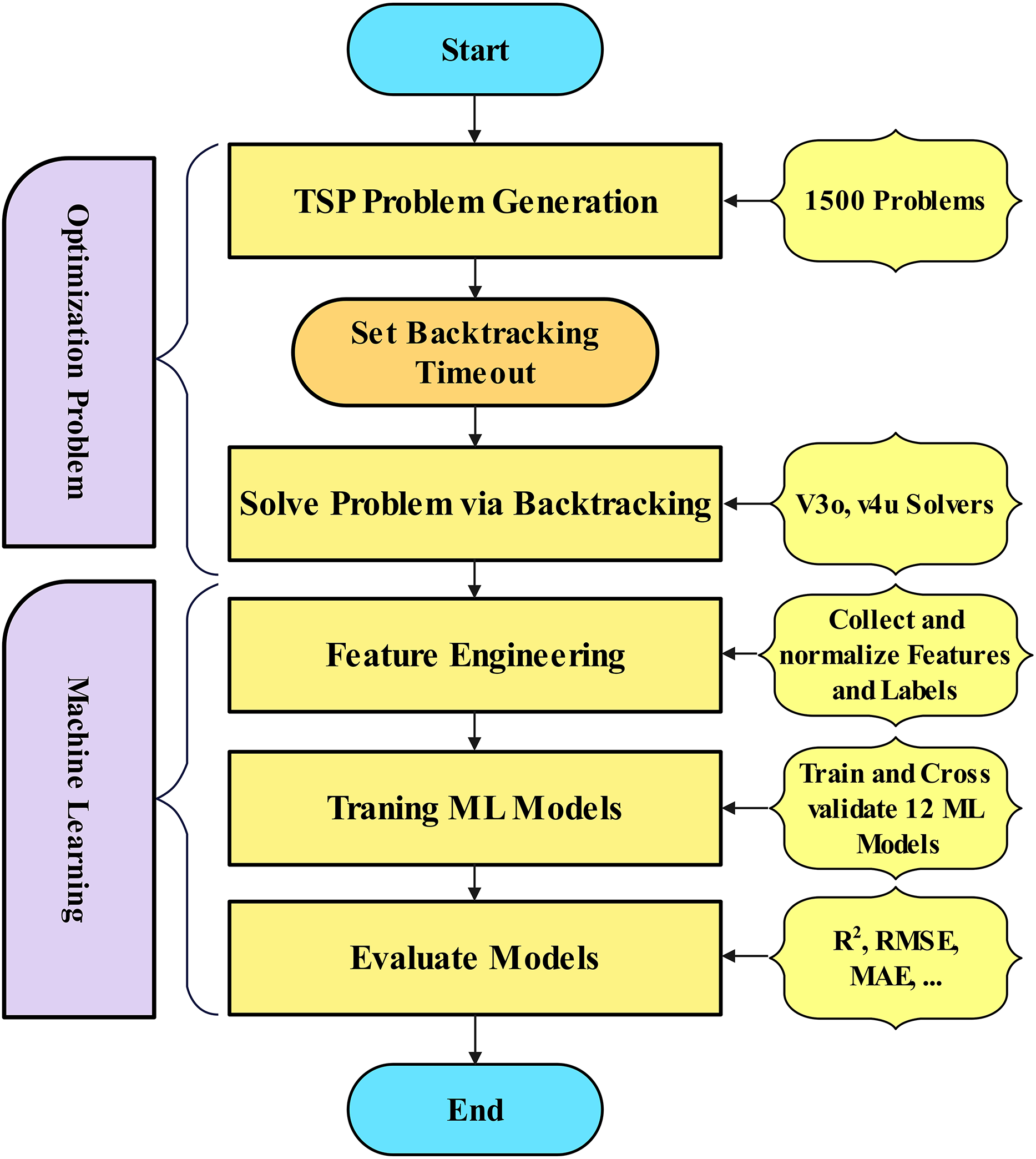
This study presents a machine-learning-based methodology for predicting the computational workload of a backtracking-based TSP solver. Figure 1 illustrates the methodology flow chart for this research, from data collection to workload estimation for the optimization problem. The methodology is as follows: problem instance generation, algorithmic solving via backtracking, feature extraction, predictive modeling, and performance evaluation.
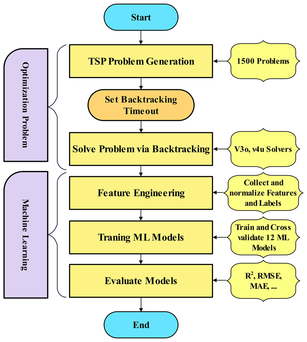
Figure 1: Research methodology for workload estimation.
Problem definition and parameterization
Each instance of the TSP was rigorously defined using structured parameters to enable workload prediction (Alanzi & Menai, 2025). The number of cities (nodes) directly affects computational space because the number of possible routes grows factorially with the number of cities. In this study, the number of cities was systematically varied to reflect problem complexities ranging from simple to highly complex. The second defining parameter is the cost matrix, which captures inter-city distances and forms the optimization objective function. The cost matrices were generated synthetically using random numerical distributions to produce realistic, computationally meaningful values. To preserve the TSP’s canonical structure, all problem instances were limited to visiting each city once and returning to the starting point. Each instance also had a predefined execution timeout to limit excessive computation time and simulate real-world resource constraints. These parameters created diverse, well-defined TSP instances that reflect realistic computational challenges (Böther et al., 2022).
Synthetic dataset creation
TSPLIB is a widely recognised benchmark set; nonetheless, it is lacking in detailed solver metrics and controlled variability for workload forecasting. A synthetic dataset was generated to ensure topological variety and document backtracking and pruning tendencies for machine learning research. To generate a large set of TSP instances for empirical analysis, a Python-based synthetic dataset generator was created based on defined problem parameters. The generator automatically generated 1,500 unique problem instances with different city counts, cost structures, and configurations. Controlled randomization ensured high variability and mathematical validity during the generation process. The resulting dataset encompasses a range of computational behaviors and problem topologies suitable for training and evaluating predictive models. To ensure compatibility with the Java-based backtracking solver and machine learning components, each instance was formatted in a standardized structure. Standardization ensured consistency across the experimental pipeline, enabling data transfer between problem generation, algorithm execution, and model training. Automated generation and strict formatting protocols create a robust dataset for modeling the relationship between TSP instance characteristics and computational workload during backtracking-based solution.
Backtracking for TSP
This study addresses the TSP using two variants of backtracking algorithms, v3o and v4u. These models differ in their node generation strategies and pruning methods. Each approach explores the space of Hamiltonian cycles by incrementally building tours from a fixed starting point and evaluating partial solutions with heuristic or bound-based criteria to decide whether to continue expansion. The overall objective is to minimize the total length of the Hamiltonian tour that visits each city exactly once and returns to the origin (Yousefikhoshbakht, 2021; Kowalik et al., 2023).
The TSP is modeled as follows. Let be a complete undirected graph, where is the set of cities and E contains weighted edges with distances for all , and . A tour is a permutation of the cities such that (fixing the origin). The total travel distance, including the return to the start, gives the cost of the tour as:
(1) The algorithm maintains a search tree where each node represents a partial tour , with an associated cost equal to the sum of distances along this partial path. The remaining unvisited cities are stored in a set , and represents the cost to return to the origin. The key to effective pruning lies in estimating the minimum additional cost required to complete the tour from any given node (Yousefikhoshbakht, 2021).
In the v3o model, the algorithm employs a heuristic candidate-selection approach based on the nearest-neighbor principle. At each search node, the remaining cities are ordered by increasing distance from the last-visited city, prioritizing the exploration of nearer cities. This heuristic ordering can help find high-quality complete tours early in the search process. However, v3o does not apply any global bounding technique to limit the search space. Pruning is used only when a complete tour is found whose cost exceeds the current best (incumbent) solution. Formally, if is the cost of the incumbent solution, a completed node is discarded if:
(2)
Because incomplete paths lack lower bounds, the v3o model may end up exploring many suboptimal regions of the search tree, especially in large-scale instances (Weinand et al., 2022). The v4u model builds upon v3o by introducing a global bounding function based on the Minimum Spanning Tree (MST) heuristic. Like v3o, it uses an ordered candidate list that prioritizes cities closer to the current location. However, in v4u, each partial node computes a bound on the minimal additional cost required to complete the tour. This bound consists of three components: the weight of an MST spanning the unvisited cities, the cost to connect the last-visited city to an unvisited city, and the cost to return from the unvisited cities to the starting city. The bound is formally defined as:
(3)
This equation allows the algorithm to prune entire subtrees when the projected tour cost exceeds the incumbent . Pruning is applied more aggressively, even for partial tours, even on partial tours:
(4)
The inclusion of bounding helps eliminate paths that cannot possibly yield an optimal tour, making the search significantly more efficient than v3o, mainly when reasonable incumbent solutions are found early due to the ordered traversal. In contrast, the v4u model adopts the same MST-based bounding technique as v4u but removes the ordering heuristic for selecting candidates. That is, instead of sorting cities in by their distance to the current city, it explores them in an arbitrary order. The lack of ordering means that optimal or near-optimal tours may not be discovered early, delaying the improvement of the incumbent and reducing the likelihood of early pruning. However, v4u still uses the exact bound computation:
(5)
The pruning rule remains:
(6)
The main advantage of v4u is that it decouples pruning from ordering, offering a different trade-off. Although it may perform less well at finding good incumbents early, it retains the strong bounding capability to exclude unpromising regions of the search space. This can be beneficial in scenarios where ordering is unreliable or adds computational overhead (Morrison et al., 2016). Together, these models demonstrate the progression in TSP-solving strategies from basic ordered backtracking (v3o) to unstructured search with strong global pruning (v4u). The comparative analysis of these models sheds light on the roles of heuristic guidance and mathematical bounding in efficient combinatorial optimization. Algorithm 1 presents the backtracking solver algorithm.
| 1: Input all parameters and data. |
| 2: Set |
| 3: Set |
| 4: Verify that all cities have been explored and returned to the starting point. |
| 5: if true then |
| 6: if then |
| 7: |
| 8: current path |
| 9: Update gradients: to minimize error |
| 10: end if |
| 11: end if |
| 12: Apply Backtrack to |
| 13: Backtrack to the preceding city. |
| 14: Mark the current city as unexplored. |
| 15: for each unexplored city do |
| 16: if then |
| 17: Mark the city as explored. |
| 18: Recursively continue exploration from this node. |
| 19: end if |
| 20: Return to the preceding city and backtrack. |
| 21: Mark the city as unexplored. |
| 22: end for |
| 23: return , , and collected feature metrics |
Feature engineering
To support this study, a specialized dataset of TSP instances was created, focusing on capturing detailed solver behavior using a backtracking algorithm. A total of 1,500 problem instances were generated through a custom Python-based solver. For each example, a set of quantitative metrics was collected to characterize the algorithm’s performance and internal operations. Importantly, the data were collected from two distinct versions of the solver (v3o and v4u), yielding two complementary datasets for comparative machine learning analysis. For each version, the recorded features include the total number of events executed (evts), the number of explicit backtracking steps taken (backtrackEvts), the number of potential backtracks avoided through pruning (pruneBacktrackEvts), and the number of pruning events where infeasible paths were eliminated (pruneEvts). Additionally, the number of optimization improvements to the current best solution (strengthenEvts) was tracked, along with the total time required to solve each instance (time), the final optimized tour length (objective), and a binary label indicating whether a given step resulted in further exploration of the search space (expand Event).
After collecting the raw data, a series of preprocessing and feature engineering steps were conducted to prepare the datasets for machine learning applications. Initially, all incomplete or null records were removed to maintain data quality. Continuous variables, particularly time and objective, are standardized (e.g., using z-score normalization) to mitigate scale differences and enhance algorithmic performance. Discrete values were encoded using label encoding. Each dataset was further enriched through expert-driven feature construction. Derived attributes, such as ratios of key event metrics (e.g., backtrack-to-prune), were created to better reflect solver dynamics. Descriptive statistics, including mean, median, and standard deviation, were computed for key metrics to capture distributional characteristics across problem instances. Furthermore, spatial features were introduced based on the proximity matrix for each TSP instance, including the average, minimum, and maximum distances between cities.
To enable robust machine learning modeling and evaluation, both datasets, v3o and v4u, were partitioned into training and validation subsets. Each was structured to be compatible with standard machine learning frameworks, ensuring efficient integration into predictive modeling pipelines. This comprehensive, version-specific data generation provides a rich foundation for analyzing and comparing solver behavior across different versions. It facilitates the development of accurate, data-driven models of TSP solution strategies.
Model development
The selected machine learning models encompass a diverse range of learning paradigms, including linear, tree-based, ensemble, and neural approaches. This was executed to ensure a just assessment of interoperability, complexity, and forecasting accuracy. These models were created to estimate the computational workload of the backtracking-based TSP solver. A wide range of regression algorithms was used to study various modeling paradigms. These modeling paradigms included linear, parametric, non-linear, tree-based, and ensemble learning. Linear Regression, Ridge, and Lasso were used as interpretable baselines. These models demonstrated how simple linear combinations of input features could capture a significant amount of variance. These models also helped benchmark the relative improvements of more complex architectures.
To model non-linear feature interactions and decision boundaries, tree-based learners were used. The Decision Tree Regressor models hierarchical splits in the data using an interpretable structure in an easy-to-interpret framework. However, the Random Forest Regressor, an ensemble of decision trees, was chosen for its bagging, which reduces variance and improves prediction stability (Thiyagalingam et al., 2022). Gradient boosting methods, such as XGBoost, LightGBM, and CatBoost, were selected for their ability to capture complex patterns through iterative refinement and regularization (Szczepanek, 2022). This makes them useful for high-dimensional, structured data. Each of these boosting models provides distinct algorithmic advantages, such as XGBoost’s regularized objective function and sparsity-aware algorithm, LightGBM’s histogram-based feature binning for efficiency, and CatBoost’s built-in support for categorical variables and ordered boosting strategy.
The analysis also included kernel-based models to evaluate their capacity to model non-linear relationships by mapping data to higher-dimensional spaces. K-Nearest Neighbors (KNN) was assessed for its simplicity and local approximation, while the Multi-Layer Perceptron (MLP) utilized a neural network to learn from complex interactions involving multiple features. The stacking ensemble model utilized Random Forest and XGBoost as base learners and Ridge Regression as the meta-learner (Ramesh & Kumaresan, 2025). This stacked framework was designed to leverage the complementary strengths of individual models and enhance generalization by mitigating model-specific biases. All models were trained using 80% of the data, with the remaining 20% reserved for validation (Hussain & Haris, 2019).
Hyperparameter tuning was conducted methodically to ensure balanced and uniform evaluation across all models. Each model was statistically optimized using scikit-learn’s GridSearchCV, which utilized a grid search with 10-fold cross-validation. To find the best configurations, the number of estimators, maximum tree depth, learning rate, regularization strength, and neural network architecture were varied. This exhaustive search ensured that every model was fairly evaluated, with sufficient training opportunities to learn from the data without overfitting.
Python was the primary programming language used for model development in the pipeline. Scikit-learn, XGBoost, LightGBM, and CatBoost were also utilized. In this environment, dataset generation and preprocessing were seamlessly integrated, and the target workload labels were implemented in Java. The Spyder IDE was used for experimentation, visualization, and result management throughout the research process to ensure transparency, modularity, and reproducibility. Table 1 summarizes the hyperparameter configurations for each model.
| Model | Hyperparameters with values |
|---|---|
| Linear regression | fit intercept=True, normalize=‘deprecated’ |
| Ridge | alpha=1.0, solver=‘auto’, fit intercept=True |
| Lasso | alpha=1.0, max iter=1,000, tol=0.0001 |
| Decision tree | max depth=None, min samples split=2, min samples leaf=1, criterion=‘squared error’ |
| Random forest | n estimators=100, max depth=None, min samples split=2, max features=‘sqrt’ |
| Gradient boosting | n estimators=100, learning rate=0.1, max depth=3 |
| XGBoost | n estimators=100, learning rate=0.1, max depth=3, colsample bytree=1.0 |
| LightGBM | n estimators=100, learning rate=0.1, num leaves=31, max depth=-1, subsample=1.0 |
| CatBoost | iterations=1000, learning rate=0.03, depth=6, l2 leaf reg=3.0 |
| KNN | n neighbors=5, weights=‘uniform’, leaf size=30 |
| MLP | hidden layer sizes=(100,), activation=‘relu’, solver=‘adam’, LR=0.0001 |
| Stacking | estimators=(‘rf’, ‘xgb’), final estimator=Ridge(), cv=5 |
Experiments and analysis
In this section, we present the effectiveness of our proposed method for predicting the computational cost of the Backtracking solver for TSP. Our implementation is executed on a Windows PC with the following specifications: Intel Core i9-13900HX (24 cores, 2.2 GHz), RTX 4090 (12 GB GPU), and 32 GB RAM. We applied our method in the following steps. A corpus of synthetic Traveling Salesman Problem (TSP) designed to reflect real-world scenarios. is generated. Each instance was solved via two backtracking processes, and metrics such as the execution time and resource usage were recorded. The efficacy of a machine learning model depends on the quality of the features used during training and on the extraction of these features for learning. Models were trained using the extracted and engineered features. To ensure optimal performance, the models are fine-tuned using the feature-engineered datasets. The trained models were rigorously evaluated to establish their robustness and reliability.
Evaluation criteria
Model performance was assessed using standard regression metrics. Let be the actual values and the predicted values: Adjusted :
(7)
Root Mean Squared Error (RMSE):
(8)
Mean Absolute Error (MAE):
(9)
Mean Relative Error (MRE):
(10)
Symmetric MAPE (SMAPE):
(11)
Accuracy within Tolerance: Percentage of predictions within 10% of actual values:
(12)
These metrics jointly capture both absolute and relative error, distributional behavior, and the model’s ability to generalize across prediction intervals (Chicco, Warrens & Jurman, 2021).
Results and discussion
To assess the predictive potential of different learning paradigms on TSP solver behavior, 12 diverse regression models were developed. These encompassed linear regressors, tree-based algorithms, ensemble learners, and neural and kernel-based approaches, each offering distinct functional capabilities and interpretive advantages. The final model suite also included a meta-learning architecture using stacking to integrate complementary predictions from base models.
The following results were obtained from the machine learning models. Tables 2 and 3 for all the machine learning models, including the Adjusted , RMSE, MAE, MRE, SMAPE, and results within 10%. The evaluation metrics are divided into two classes of evaluation, for Adjusted , where higher values indicate better performance (up to 10% improvement preferred). In contrast, lower values indicate better performance for the remaining metrics. Table 2 describes the results of the v3o backtracking model, whereas Table 3 illustrates the results of the v4u model, which compares regression models for Traveling Salesman Problem computational effort in backtracking-based TSP solving. Model selection and validation are essential, while others underperform or lack generalizability.
| Model | Adjusted | RMSE | MAE | MRE | SMAPE | within10% |
|---|---|---|---|---|---|---|
| Linear regression | 1.00 | 0.00 | 0.00 | 0.00 | 0.00 | 100.00 |
| Ridge | 1.00 | 0.00 | 0.00 | 0.00 | 0.00 | 100.00 |
| Lasso | 1.00 | 32.67 | 8.76 | 0.00 | 0.06 | 100.00 |
| MLP | 1.00 | 10,689.58 | 2,971.16 | 0.08 | 8.31 | 69.29 |
| Gradient boosting | 1.00 | 24,180.73 | 3,936.01 | 0.07 | 6.12 | 87.95 |
| Random forest | 0.99 | 26,836.26 | 3,980.19 | 0.01 | 0.73 | 99.32 |
| Decision tree | 0.99 | 40,386.72 | 4,949.67 | 0.01 | 0.94 | 99.09 |
| XG boost | 0.98 | 48,611.85 | 7,557.93 | 0.03 | 2.87 | 96.89 |
| KNN | 0.98 | 49,707.55 | 9,790.31 | 0.06 | 6.22 | 79.83 |
| Stacking | 0.98 | 45,342.75 | 14,332.89 | 3.86 | 109.21 | 22.97 |
| Cat boost | 0.97 | 57,953.47 | 9,543.07 | 0.25 | 20.20 | 52.09 |
| Light GBM | 0.87 | 124,969.06 | 21,465.01 | 0.12 | 8.09 | 88.25 |
| Model | Adjusted | RMSE | MAE | MRE | SMAPE | within10% |
|---|---|---|---|---|---|---|
| Linear regression | 1.00 | 0.09 | 0.01 | 0.00 | 0.00 | 100.00 |
| Ridge | 1.00 | 0.09 | 0.01 | 0.00 | 0.00 | 100.00 |
| Lasso | 1.00 | 0.48 | 0.19 | 0.00 | 0.05 | 100.00 |
| MLP | 1.00 | 324.84 | 52.01 | 0.01 | 0.69 | 99.85 |
| Gradient boosting | 0.81 | 594,202.19 | 37,589.35 | 0.35 | 17.33 | 73.41 |
| Random forest | 0.80 | 598,806.19 | 37,603.76 | 0.01 | 1.18 | 99.32 |
| Decision tree | 0.80 | 600,320.85 | 37,855.47 | 0.01 | 0.82 | 99.55 |
| XGBoost | 0.78 | 602,519.71 | 39,086.05 | 0.05 | 4.56 | 90.45 |
| KNN | 0.77 | 615,948.22 | 38,964.63 | 0.01 | 0.96 | 99.24 |
| Stacking | 0.61 | 642,065.89 | 43,977.66 | 1.39 | 58.20 | 22.65 |
| Cat boost | −0.06 | 749,618.08 | 74,115.37 | 4.83 | 123.65 | 4.17 |
| Light GBM | −4.16 | 896,236.91 | 89,069.24 | 2.84 | 16.07 | 78.79 |
The Linear Regression and Ridge Regression models performed well, with an Adjusted R-squared value of 1.00 and zero % error in RMSE, MAE, MRE, and SMAPE. Although these results appear better, they may be due to overfitting or deterministic correlations. The feature space may contain all the target-variable information, or the test cases may be too close to the training data, reducing the model’s applicability to more complex or undiscovered TSP situations. The Lasso Regression model with L1 regularization achieved an adjusted R-squared value of 1.00 and a moderate error (RMSE = 32.67, MAE = 8.76), demonstrating improved resistance to overfitting compared to the unregularized models. The ensemble tree models, including XGBoost and Random Forest, show strong generalization performance on unseen data. The Random Forest model achieved an Adjusted of 0.99, an MAE of 3980.19, indicating solid predictive accuracy, and 99.32% correct predictions within 10% of the actual workload. Decision Tree models showed that hierarchical splits can capture functional patterns in simpler instances, and hierarchical feature splits can effectively solve most workload estimation problems, even in simple scenarios. The ensemble XGBoost achieved 96.89% accuracy in predicting moderately complex nonlinear relationships within 10%.
Neural network-based approaches, such as the MLP, exhibited higher error rates and a significantly lower percentage of accurate predictions within 10% (69.29%). MLP performance is sensitive to hyperparameters, especially under low-data or low-feature-redundancy conditions. The high RMSE and MAE of KNN were likely due to the potential for poor generalization of local structure in high-dimensional or irregular feature spaces. The high SMAPE (109.21) and MAE (14,332.89) of the stacking model suggest that its base learners are overfitting. Light GBM, a well-known boosting technique, showed the highest RMSE (124,969.06), the lowest Adjusted (0.87), and a high SMAPE (8.09), indicating poor predictive performance for workload estimation. CatBoost, which performed well on other structured learning tasks, struggled with this dataset (Adjusted = 0.97, SMAPE = 20.20) due to inadequate learning dynamics, misinterpretation of categorical inputs, or incorrect assumptions about how categorical features are processed.
In backtracking-based TSP solvers, XGBoost and Random Forest were the most effective methods for accurately estimating computing effort. These models offer strong reliability for real-world workload-estimation applications, benefiting from their robust prediction accuracy and resistance to overfitting.
Table 3 shows the evaluation of the v4u dataset. A clear performance difference was observed between the models’ assessment of the v4u feature representation and the previous v3o results. Once more, the results of the linear models Ridge, Lasso, and Linear Regression were better (Adjusted = 1.00, with zero or negligible error), demonstrating that the data had strong linear correlations. However, concerns are raised about overly simple target-feature relationships that do not generalize to unseen TSP instances, as consistently high precision across both datasets may reflect overfitting or a lack of generalizability.
Neural networks (MLPs) also demonstrated remarkable performance on v4u, achieving 99.85% accuracy within a 10% error margin. This indicates that the feature set is well-aligned with MLP’s capabilities; however, this may reflect overfitting rather than true generalization. On v4u, however, ensemble methods such as LightGBM, Random Forest, XGBoost, and Gradient Boosting showed a notable decline in performance. RMSE values increased (e.g., despite excellent v3o results). For example, Gradient Boosting showed an RMSE exceeding 594,000, and Adjusted dropped to approximately 0.8 or lower. This suggests that the non-linear structure needed for effective generalization by tree-based models is absent from v4u features. Due to their high SMAPE and negative values, Cat Boost and Light GBM performed particularly poorly, indicating incompatibility with their learning mechanisms. Random Forest and Decision Tree maintained high prediction accuracy within 10% (99%), despite higher RMSE values within 10% ( 99 percent), suggesting localized prediction accuracy that is sensitive to outliers. Consistent with previous findings, stacking once again failed to generalize effectively.
The v4u feature structure favors linear models but hinders the performance of more complex ones. This highlights the importance of feature engineering that captures non-linearities for accurate workload estimation in TSP solvers. The primary goal of this method is to be practical, interpretable, and applicable, while providing clear guidelines for resource allocation and algorithm selection.
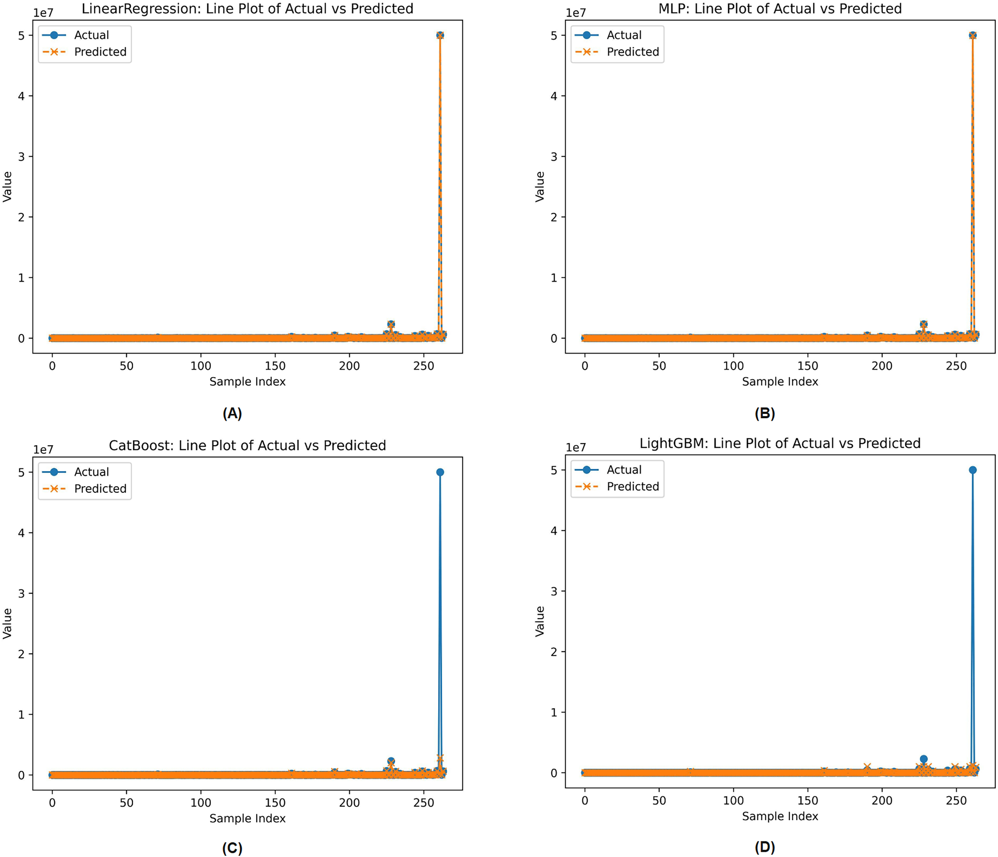
Line plots of actual against projected values were used to compare the best and worst machine learning models based on preset assessment parameters in Fig. 2. These models were selected from the complete set of evaluated machine learning models. Figure 2 illustrates the performance of Linear Regression, Multi-Layer Perceptron (MLP), CatBoost, and LightGBM. All models are evaluated based on how well they align with the actual distribution of the target variable. Linear Regression and MLP appear to most closely match the actual values across all sample indices, indicating robust performance. However, Cat Boost and Light GBM deviate significantly from the actual values, especially for samples with high target values, indicating a lack of generalization in key areas.
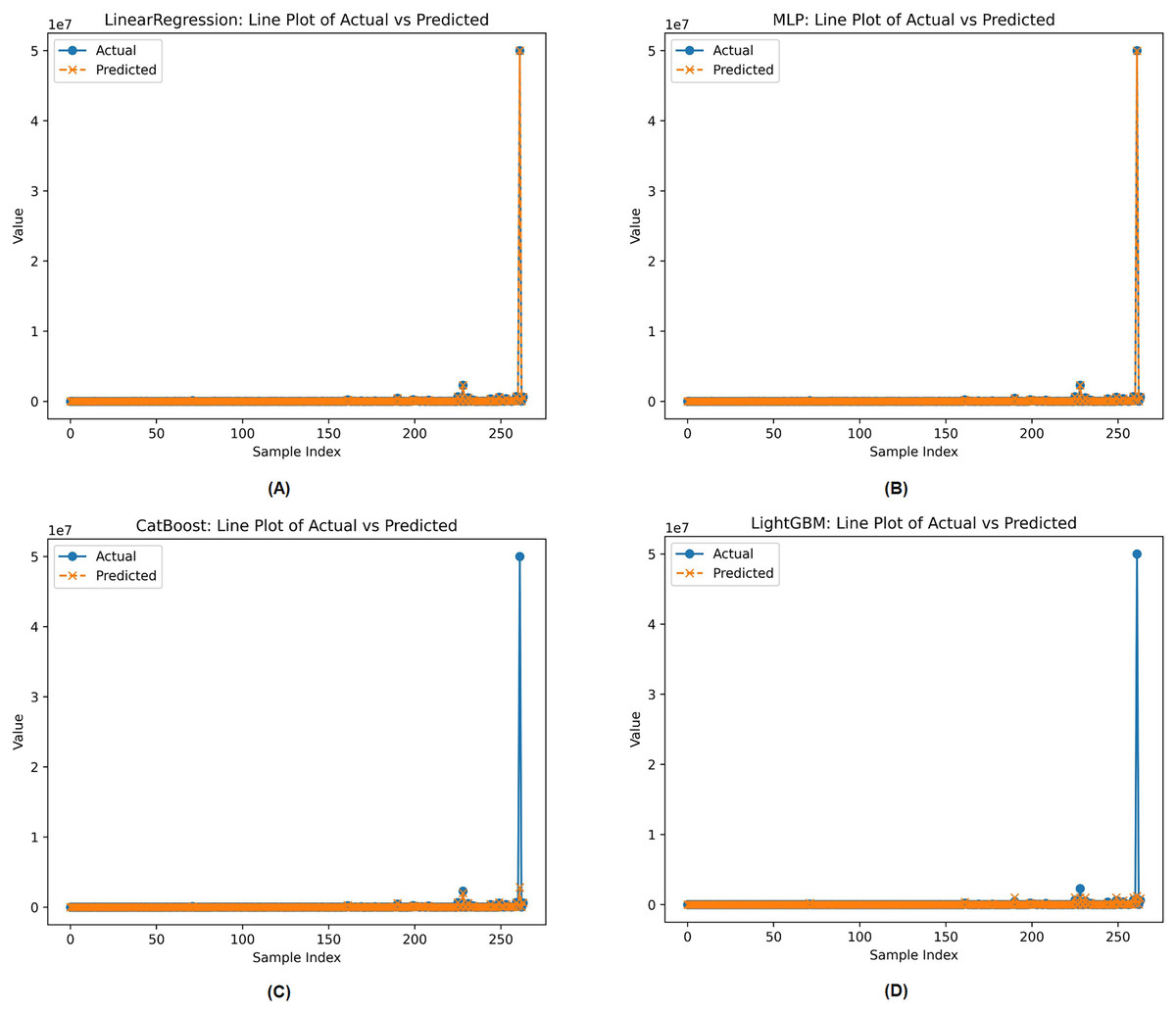
Figure 2: Actual vs. predicted workload for the two best (Linear regression, MLP) and the two worst (Cat Boost, Light GBM) models on the v4u dataset.
Each model handles data complexity and outliers differently, which explains these performance disparities. Linear Regression and MLP show greater extrapolation stability when properly regularized and trained, allowing them to align with absolute values even with extreme predictions. MLP’s non-linear modeling potential may help explain its high predictive accuracy. However, CatBoost and LightGBM may struggle with highly skewed or severely skewed target distributions in regression.
This is especially true if models are not calibrated to handle outliers. Tree-based models often average predictions across weak learners, which can suppress extreme values, unless they are designed to incorporate such variance. Additionally, poor training data in regions with high target values may have caused underrepresentation in leaf nodes, skewing predictions toward the mean. Given this, model adjustment, resampling strategies, or transformation approaches are needed to prevent performance degradation in specific locations. Synthetic datasets for diverse TSP topologies have reduced problem diversity, while specific configurations may fail to accurately reflect real-world variability. Future research could enhance model generalization by using a broader range of diverse or experimentally derived topologies.
Time comparison
Figure 3 compares training times between models in v3o and v4u, highlighting improved computational efficiency, especially in v4u. Linear Regression, Ridge, and Lasso maintained training times at 0.01 s. This demonstrates their efficacy in rapid model deployment and resource environments.
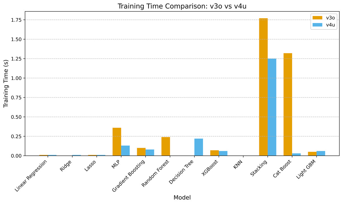
Figure 3: Time comparison of all models on v3o vs. v4u.
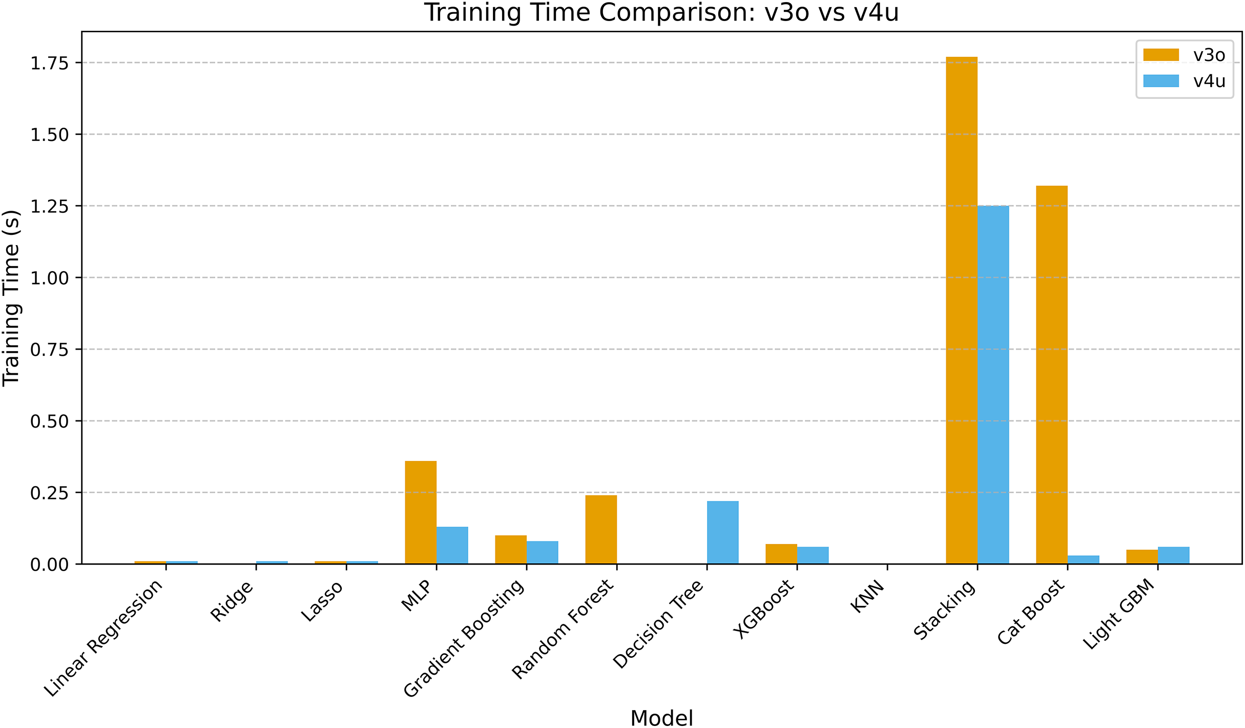
The time for MLP training decreased from 0.36 to 0.13 s, indicating improved optimization or hardware acceleration. Despite being ensemble-based, stacking also reduced training time from 1.77 to 1.25 s, demonstrating v4u’s improved meta-model architecture. CatBoost’s training time dropped from 1.32 to 0.03 s. This is an order-of-magnitude improvement, indicating that v4u implemented framework-level enhancements or more efficient categorical encoding. The increase from negligible to 0.22 s is possibly due to a more detailed tree construction or preprocessing strategy. Gradient Boosting, XGBoost, and LightGBM exhibited consistent training profiles across both versions, indicating maturity and well-optimized implementations. v4u improves training efficiency, especially for neural and ensemble-based models. Therefore, it is well-suited for iterative experimentation and deployment at scale.
Conclusion
This study proposed a machine learning framework to predict the computational workload required to solve instances of the Traveling Salesman Problem using backtracking algorithms. Unlike traditional methods that treat each instance uniformly, our method enables pre-execution workload estimation, which facilitates intelligent solver selection and resource allocation. Two backtracking models, v3o and v4u, with different pruning strategies and search behaviors, were implemented. A 1,500-problem synthetic dataset was used to capture results from both solver datasets, including backtrack events, pruning actions, and optimization steps. Thirteen regression models were developed and evaluated using standard metrics, including , RMSE, MRE, SMAPE, and the percentage of predictions within 10% of the actual values. Both solver datasets show that Random Forest and XGBoost perform better. On the v3o dataset, the Random Forest algorithm had an Adjusted of 0.99, and 99.32% of predictions fell within a 10% margin of the actual values. The XGBoost algorithm achieved an accuracy of 96.89%. Linear models achieved a perfect score (Adjusted = 1.00) in the v4u dataset, although their generalization to unseen data remains under evaluation. MLP modeled feature-rich nonlinear dynamics well on v4u, achieving 99.85% accuracy with a 10% margin of error. The findings demonstrate that machine learning can estimate solver workload from structural instance features, thereby bridging traditional optimization techniques with predictive modeling. This method reduces computational overhead and supports data-driven, adaptive combinatorial optimization decisions. The system demonstrated commendable performance on synthetic datasets; however, incorporating real-world TSP examples could enhance its adaptability and resilience. This would enhance its practical utility in additional optimization fields. The novelty and effect of this study stem from its data-driven approach that combines machine learning with backtracking-based TSP solvers for pre-execution workload prediction. This approach advances intelligent solver selection and resource optimization in combinatorial optimization research. Next, this framework may be extended to include real-world TSP variants, dynamic feature extraction, and application to more general NP-hard logistics, scheduling, and network optimization problems.